Sensitivity of Common Vegetation Indices to the Canopy Structure of Field Crops


1
Collaborative Innovation Center on Forecast and Evaluation of Meteorological Disaster, School of Geography and Remote Sensing, Nanjing University of Information Science & Technology, Nanjing 210044, China
2
Land Remote Sensing, VTT Technical Research Centre of Finland Ltd., P.O. Box 1000, FI-02044 VTT Espoo, Finland
*
Author to whom correspondence should be addressed.
Remote Sens. 2017, 9(10), 994; https://doi.org/10.3390/rs9100994
Submission received: 20 August 2017
/
Revised: 19 September 2017
/
Accepted: 21 September 2017
/
Published: 26 September 2017
(This article belongs to the Section Remote Sensing in Agriculture and Vegetation)
Abstract
:Leaf inclination angle distribution is an important canopy structure characteristic which directly impacts the fraction of the intercepted solar radiation. Together with the leaf area index (LAI) it determines the structure and fractional cover of a homogeneous crop canopy. Unfortunately, this key canopy parameter has usually been ignored when applying common multispectral vegetation indices to the mapping of LAI, although its impact is known from model simulations. Therefore, we measured leaf angles and determined their distribution (quantified using the leaf mean tilt angle, MTA) for six crop species with different structures growing on 162 plots with a broad range of LAI (1.1–5.0) and leaf chlorophyll content (26–94 μg cm−2). Next, we calculated six vegetation indices widely used for LAI monitoring—the normalized difference vegetation index (NDVI), the enhanced vegetation index (EVI), the two band enhanced vegetation index (EVI2), the modified triangular vegetation index (MTVI2), the optimized soil adjusted vegetation index (OSAVI) and the wide dynamic range vegetation index (WDRVI)—from airborne imaging spectroscopy data. We calculated the Spearman’s correlation coefficient , a non-parametric statistic chosen because of the non-normal distribution of canopy parameters. All studied indices depended on the LAI (, but the dependence on the MTA was of similar magnitude ( with EVI, EVI2, OSAVI and MTVI2 depending more strongly on MTA than on LAI. All studied indices were good proxies ( for vegetation fractional cover (Fcover) which, for homogeneous crop canopies, is a nonlinear function of LAI and MTA. EVI2 and MTVI2 were the most strongly correlated with Fcover, although the difference to the other studied indices was small. This first study involving a large range of crop structures confirms the results from canopy reflectance simulations and emphasizes the necessity of leaf angle information for the successful mapping of LAI with Earth observation data.
Keywords:
canopy structure; mean tilt angle; leaf angle distribution; imaging spectroscopy; NDVI; EVI; EVI2; MTVI2; OSAVI; WDRVI; PROSAIL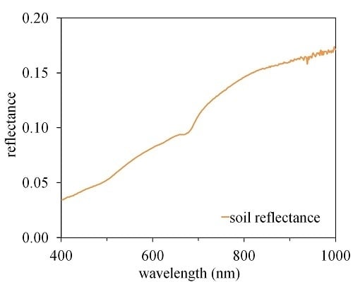
1. Introduction
Canopy structure, or its architecture, is understood as the spatial distribution and orientation of vegetation components within a canopy. It directly affects the interception of solar radiation and thus also how radiation is reflected or intercepted by the canopy. Vegetation structure has an effect on land surface energy balance and it influences leaf temperature, photosynthetic activity and plant growth [1,2,3,4]. Vegetation structure thus plays a dual role in remote sensing. First, it is a canopy characteristic which needs to be retrieved to understand biophysical processes. Second, due to its direct effect on canopy reflectance, it needs to be taken into account—and corrected for—when other canopy biophysical or biochemical variables are determined from remote sensing data.
The complexity of canopy structure varies with biome and plant functional type. Crop canopy is usually assumed to be the simplest possible case—horizontally homogeneous and with a constant distribution of leaf normals, i.e., the vertical profile of the canopy is the same at all locations. Its structure can thus be described by the amount of leaves above the unit horizontal ground area and their directional distribution, which can be quantified using the leaf area index (LAI) and leaf angle distribution (LAD), respectively. LAI is a key variable for understanding the biophysical characteristics of the vegetated areas of the planet [5,6,7]. For agricultural management, crop LAI measured over large areas can be used to estimate productivity on national to global scales. The other structural characteristic, LAD, quantifies the distribution of the angles between leaf normals and the vertical direction. If the azimuth angles of leaves are uniformly distributed, LAD and LAI completely determine the transmission of radiation through the canopy [8]. Compared with LAI, much less attention has been paid to LAD when describing the biophysical characteristics of vegetation.
Spectral vegetation indices (VIs), calculated from canopy reflectance in a small number of selected spectral bands mostly in the visible and near infrared (NIR) spectral domains [9,10,11,12], are commonly used for the remote estimation of vegetation biophysical characteristics. Visible bands are utilized for determining the absorption by plant pigments active in this spectral region, whereas the reflectance in the NIR domain, where green leaves have minimal scattering, contains information on canopy cover and thickness. However, in addition to the number of leaves, canopy reflectance is also affected by many factors, such as soil background, atmospheric effects, canopy element optical properties and canopy architecture.
Despite its central role, there is a noticeable lack of empirical evidence on the effect of LAD on even the most common VIs. The main reason is likely a lack of in-situ measurements of canopy LAD, or the central moment of the distribution, the mean tilt angle (MTA). A traditional direct approach for LAD measurement is using clinometers in contact with the leaf surface [13]. This method is laborious and time consuming, and direct measurement is inevitable to disturb the leaf natural orientation. Indirect leaf mean tilt angle estimation relies on the inversion of the gap fraction below the canopy [14]. Some specialized techniques were applied to characterize 3D canopy structure, e.g., portable laser canning [15,16], which were resource demanding and rigid to operate. A digital photography method was developed to estimate the LAD of tree species [17,18,19] and extended and validated for field crops [20].
The effect of MTA is obvious across the whole optical spectrum as this parameter affects canopy transmittance in both the view and illumination directions and thus the brightness and visibility of the vegetation background. An especially strong dependence of reflectance on MTA has been found in the far-red edge spectral region, around 750 nm [21,22]. However, this spectral region is not included in most satellite instruments for which data is commonly available, and hence also in the most widely used VIs. We therefore point our focus on the effects of LAD on the most common wavelength combinations in the visible spectrum and NIR used in vegetation remote sensing.
A number of VIs have been developed for estimating LAI by establishing statistical relationships between VIs and measured LAI for various vegetation types. The most obvious first choice is the normalized difference vegetation index (NDVI) [23] which reflects the fractional absorbed photosynthetically active radiation and exhibits a strong relationship with vegetation characteristics [24,25,26]. This classic VI based on reflectance in red and NIR bands has numerous modifications aimed at improving robustness under varying atmospheric and background conditions, as well as linearity with specified biophysical variables. We included in this study the enhanced vegetation index (EVI) [27], which includes also reflectance in the blue band, the two-band version of EVI (EVI2, [28]), OSAVI [29], the modified triangular vegetation index (MTVI2) [30], which also includes a green band, and WDRVI [31,32]. All these indices have reported dependencies on MTA at low to middle LAI [33], based on simulated reflectance spectra. To our knowledge, the relationships have not been tested using empirical data covering a wide range of canopy structures.
The purpose of our study was to determine the role of two key canopy structural variables, MTA and LAI, in determining the values of commonly used and robust vegetation indices under actual field conditions. We measured the leaf angle distributions and reflectance properties of 162 study plots growing six different species with a large variation in both LAI and MTA. To generalize and validate the accuracy of our field-measured data, we also applied a common canopy reflectance model with inputs taken from spectral and structural measurements at the test site.
2. Materials and Methods
2.1. Study Area and Field Measurements
This study was carried out at the Viikki agricultural test field located in Helsinki (Finland) (60.224°N, 25.021°E). The size of the research area was approximately 4 km × 4 km. The annual average temperature in Helsinki is 6 °C; in July, the average temperature is 18 °C. Six crop species were included in this study growing on 162 plots: faba bean (Vicia faba L. “Kontu”), narrow-leafed lupin (Lupinus angustifolius L. “Haags Blaue”), turnip rape (Brassica rapa L. ssp. oleifera (DC.) Metzg. “Apollo”), wheat (Triticum aestivum L. emend Thell. “Amaretto”), barley (Hordeum vulgare L. “Streif”, “Chill” and “Fairytale”) and oat (Avena sativa L. “Ivory” and “Mirella”). The largest plots were 600 m2 (50 m × 12 m) and the smallest ones 20 m2 (10 m × 2 m). The soil types in the area were fertile luvic stagnosol, haplic gleysol and sulfic cryaquept. The plots differed in seeding density (55–700 m−2) and fertilizer treatment (0–150 kg N m−2) leading to LAI range of 1.1–5.0 and a chlorophyll content range of 26–94 μg cm−2 (see the Table 1 in the reference [20]).
Canopy leaf-angle distribution was determined using the photographic approach [17], validated and extended to field crops [20] on 6 July 2012 in the same growth stage as during the spectroscopy measurement. Canopy photographs were taken using a Nikon D1X digital camera mounted on a tripod and leveled with bubble level outside of the plots approximately 1 m away from the edge of the field. The camera height was between 30 and 50 cm depending on crop height. Five to six photographs were taken for each species from one or several plots. Finally, the inclination angles of 75–100 leaves or leaf fragments oriented perpendicularly to the viewing direction were measured using ImageJ 1.47 software, which is an open source image processing program [34], and used for the calculation of the leaf mean tilt angle (MTA). We assumed LAD to be species-specific, as it has been shown to vary more among species than within species [8,13,35]. A more detailed description of the test site and the photographic method was given by Zou et al. [20].
Airborne spectroscopy imagery covering the study area was acquired using an AISA Eagle II imaging spectrometer (Specim Ltd., Oulu, Finland) on 25 July 2011. The data were collected between 09:36 and 10:00 local time at approximately 600 m above ground. The flight direction was parallel with the sunrays. The solar zenith angle varied between 50.4° and 48.1° and the measurement zenith angle between 0 and 18.9° was determined by the swath width of the sensor and aircraft orientation changes. Reflected radiation was measured in 64 channels in the visible and NIR spectrum (400–1000 nm) with a spectral resolution of 9–10 nm and a spatial resolution of 0.4 m. The spectroscopic imagery was radiometrically calibrated using the CaliGeo 4.9.9 software package (Specim Ltd., Oulu, Finland) and georectifed using Parge (ReSe Applications Schläpfer, Wil, Switzerland). Finally, the radiometric data were converted to top-of-canopy hemispherical-directional reflectance factors using ATCOR-4 (ReSe Applications Schläpfer, Wil, Switzerland). The spectroscopic data were extracted from the imagery and averaged as average plot spectra.
A SunScan ceptometer (Delta-T Devices, Cambridge, UK) was used to measure LAI in the field. The data used in this study were collected within five days of the airborne campaign. The SunScan ceptometer bar was entered from the edge of the plot at approximately 45° to the row direction to minimize the row effects on LAI measurement as suggested in the instrument manual. LAI was calculated from the measured transmittance following the model implemented in the SunScan hardware. The possibility of light transmitted through the canopy at polar angle can be modeled for a random spatial distribution element canopy using an exponential model:
where is the leaf absorptivity for light set to 0.85 in this study (SunScan SSI user manual) and is the canopy directional light extinction coefficient depending on LAD. The canopy transmittance model used by SunScan uses an ellipsoidal LAD model depending on the single parameter to characterize LAD. Commonly, is assumed to have equal unity corresponding to random distribution of leaf normals due to a lack of information on the actual LAD. In this study, we calculated from the measured MTA using the following function derived from Equation (16) in [36]:
For an ellipsoidal leaf angle distribution model, can now be calculated as [13]:
The calculations were performed as follows. First, we determined MTA from the measured leaf angles. Next, we calculated the species-specific ellipsoidal leaf angle distribution parameter from Equation (2) and two extinction coefficient values from Equation (3): corresponding to the solar zenith angle at the time of the SunScan measurements, and for the nadir direction. To obtain the LAI, we solved Equation (1) for LAI and used the SunScan-measured and . Finally, the LAI for each plot was averaged from 4–5 sequential SunScan readings. We used the LAI value for each plot to calculate the fraction of the canopy cover as:
where the light transmission in the nadir direction, , was calculated from Equation (2) with . Fcover can also be directly related to SunScan measurements. After making all the substitutions listed above, we can write an equation relating Fcover and SunScan-measured transmittance measurements:
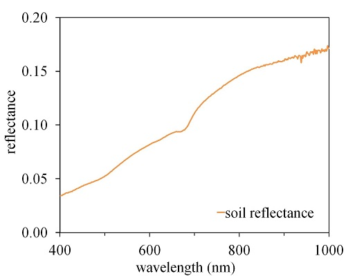
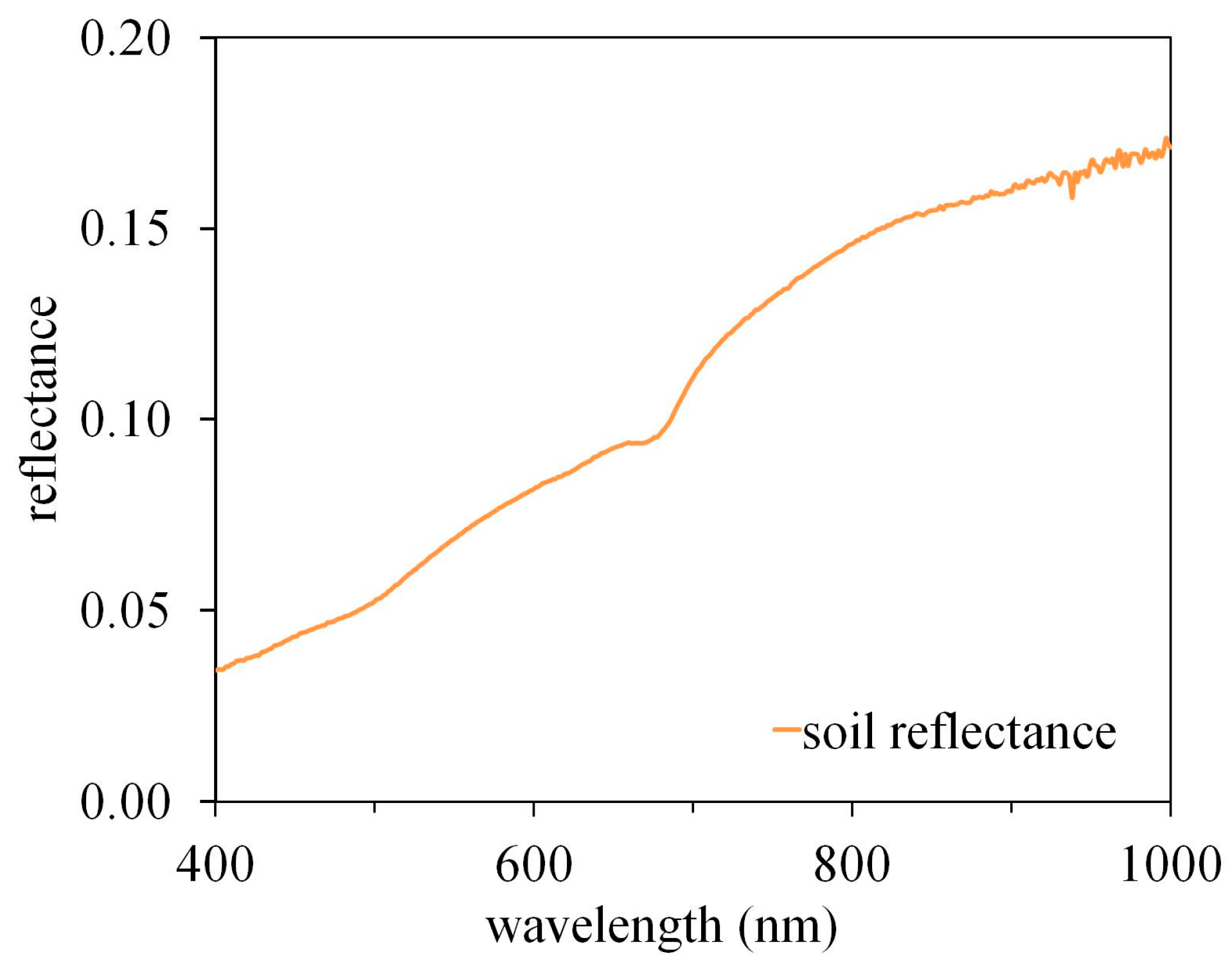
A portable spectroradiometer (ASD Handheld, Boulder, CO, USA) with spectral range between 325 and 1075 nm and a spectral resolution of 3 nm was used to measure the bare soil reflectance in four sample plots in a harvested area on 7 October 2011. Bare soil reflected radiation was collected at a distance approximately 40 cm above the soil surface and a field of view of 25°. Soil reflectance was calculated as the ratio of soil-reflected radiance to that measured above a calibrated white Spectralon panel (Labsphere Inc., Sutton, NH, USA). Due to the different solar illumination conditions between soil spectral and airborne spectral measurements, the measured soil reflectance was corrected with a bidirectional reflectance distribution function (BRDF) model developed by Walthall et al. [37] and modified by Nilson and Kuusk [38]. The soil spectrum used for PROSAIL model simulation is presented in Figure 1.
2.2. Vegetation Indices
The VIs (Table 1) used in the study (NDVI, EVI, EVI2, MTVI2 and OSAVI) make use of a total of four spectral bands (blue, green, red, and NIR) available in most modern satellite remote sensing instruments. The corresponding wavelengths used in the study are blue: 470 nm, green: 550 nm, red: 680 nm and NIR: 800 nm. As these exact wavelengths were not available in the AISA data, we used the closest available wavelength. The actual wavelengths used in the analysis were 470 nm, 551 nm, 682 nm, and 795 nm, respectively.
2.3. PROSAIL Simulations
We studied the sensitivity of the VIs to canopy structure (MTA and LAI) using the PROSAIL canopy reflectance model. The model is a combination of the leaf optical reflectance model PROSPECT-5 [39] and the canopy reflectance model SAILH [40,41]. The PROSPECT-5 model simulates leaf reflectance and transmittance from six input parameters: leaf chlorophyll a and b content (), leaf carotenoid content (), leaf dry matter content (), leaf water content (), leaf brown pigment content (), and the mesophyll structure parameter . The SAILH sub-model simulates canopy reflectance using LAI, MTA, hot spot size parameter, soil reflectance, solar zenith angle, sensor view angle, sensor azimuth angle and the fraction of incident diffuse sky radiation. The leaf inclination angle distribution is characterized from the leaf mean tilt angle to generate an ellipsoidal leaf angle distribution [42].
First, to illustrate the effects of LAI and MTA on VIs, we varied the MTA between 15 and 75 degrees, set the LAI value to 1, 3 and 5, and set all other parameters to values characteristic of healthy green vegetation: , , . Other parameters were fixed to values taken from the literature: (the average value of the six species [43,44,45,46]), (the average value of various crops [27]), (assuming the leaves were green during the measurements), and the hot spot parameter was set to 0.01 (this parameter has no practical influence on the results as the view direction was far from the hot spot because of low sun). The fraction of diffuse radiation was calculated using the 6S atmosphere radiative transfer model [47] from actual observation geometry and nearby sun photometer measurements. The parameters describing the illumination and view geometry in the model were set to coincide with the airborne spectroscopy imagery acquisition: solar zenith angle 49.4°, sensor zenith angle 9°, and azimuth angle 90°.
Next, we generated 100,000 parameter combinations by uniformly sampling the variation ranges of , , LAI and MTA within the measured (for field-measured parameters) or natural variation range (for parameters for which this information was available). According to measurements [20], varied between 25 and 100 μg cm−2, LAI between one and five, and MTA between 15 and 70 degrees (MTA = 15, 30, 40, 50, 60 and 70°). varied in a wide natural range of the parameter, between 0.001 and 0.020 cm; was linked to as 1:5 based on the LOPEX93 dataset [48].
2.4. Statistical Analysis
We analyzed the correlation between VIs and canopy parameters (LAI, MTA and Fcover) for model simulations and empirical data using the Spearman’s correlation coefficient (−1 ≤ Rs ≤ 1) which is a statistical measure of the strength of the relationship between paired data. Its interpretation is similar to that of Pearson’s correlation coefficient: the closer the Rs is to ±1 the stronger the correlation. Unlike Pearson’s R, there is no requirement of normality and assumption of a linear relationship between the two variables.
3. Results
In the modeled data for typical healthy green vegetation, all indices showed a clear and mostly negative dependence on MTA (Figure 2). The curves were most similar for the lowest LAI value, LAI = 1. At medium LAI values (LAI = 3) of the three LAI levels, the indices showed a smaller dependence on MTA. Also, the curves in Figure 1 become nonlinear and indicate lower dependence on MTA at low MTA values. The latter is especially evident for NDVI (Figure 2a) and WDRVI (Figure 2f). At LAI = 5, the nonlinearity was even larger compared with lower LAI values. The dependence of NDVI and WDRVI on MTA was slightly positive for the smallest MTA values. However, the dependence was very small and for practical purposes, NDVI and WDRVI were insensitive to the variation of MTA between below MTA = 50° for large LAI values. The other indices, EVI, EVI2, OSAVI and MTVI2, were still highly sensitive to MTA (Rs > 0.6) even at LAI = 5.
All indices showed a monotonic dependence on LAI when all other inputs in the PROSAIL model (see Section 2.3) were fixed to the values of green healthy vegetation (Figure 2). The dependence, measured as the distance between the lines in Figure 1, generally decreased with LAI and MTA. For NDVI, the lines for LAI = 3 and LAI = 5 nearly intersect at MTA = 15° indicating a lack of dependence of the index on LAI. This well-known saturation with LAI, however, is not present in EVI, EVI2 and MTVI2, for the LAI intervals investigated here.
In the 100,000 simulations (Figures S1–S3) and empirical data, the results visualized in Figure 2 were corroborated: VIs showed generally stronger correlations with MTA than LAI (Table 2). The only exceptions were NDVI and WDRVI, for which the correlation with LAI was stronger than with MTA in both datasets; for NDVI, the correlation with LAI was stronger than with MTA in the field-measured data. However, even the strongest correlations with LAI, (simulated dataset: and measured dataset: ) for NDVI and WDRVI were weaker than the strongest correlation (simulated dataset: and measured dataset: ) for EVI, EVI2 and MTVI2.
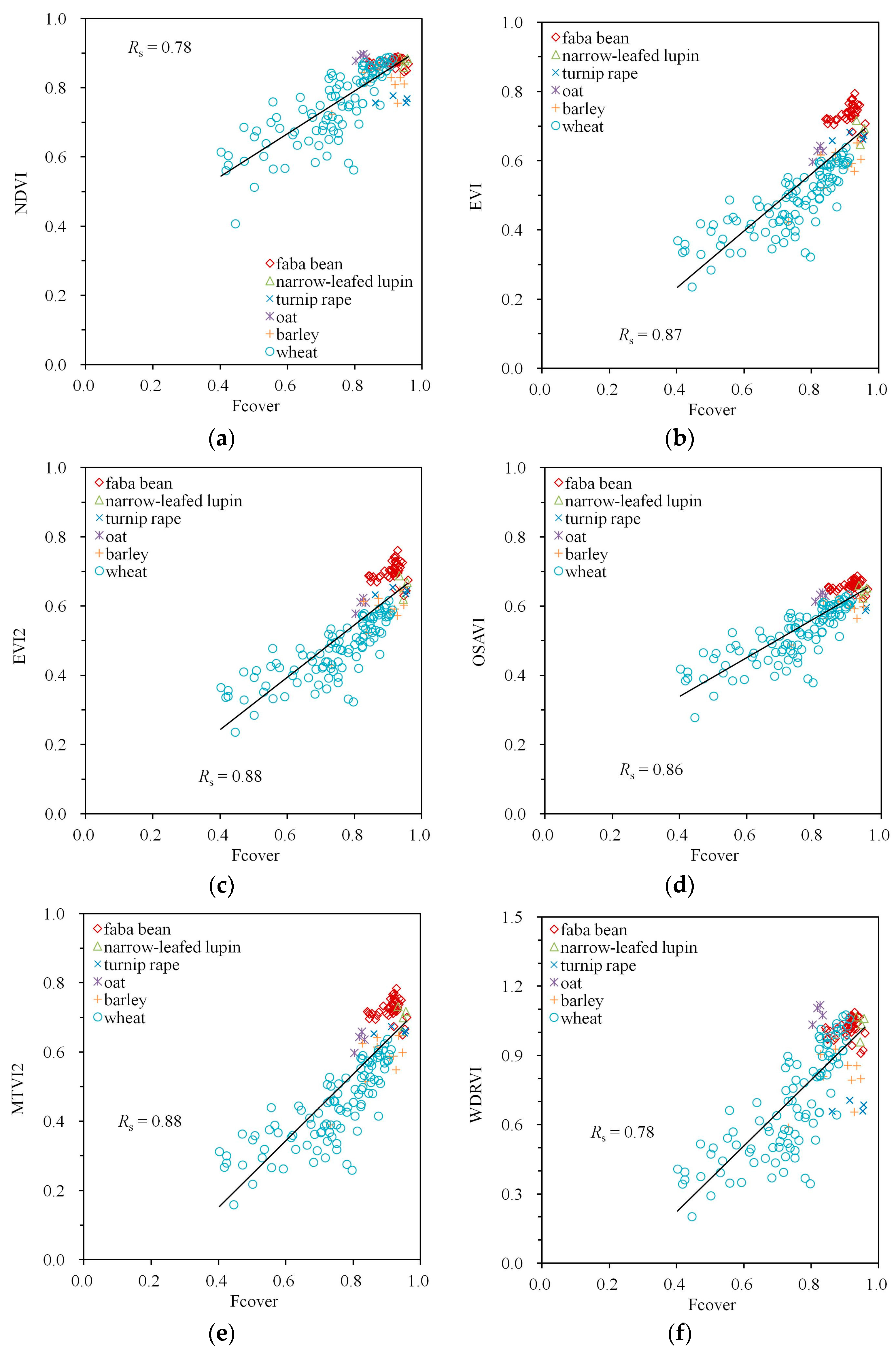
The strongest correlations in both the simulated and measured datasets were found between all studied indices and Fcover (Table 2). In the simulated dataset, was consistently above 0.93 with , indicating a near-perfect correlation for NDVI and WRDVI. In the measured data, the values of were somewhat smaller, around 0.8, with the lowest value () produced by NDVI and WRDVI.
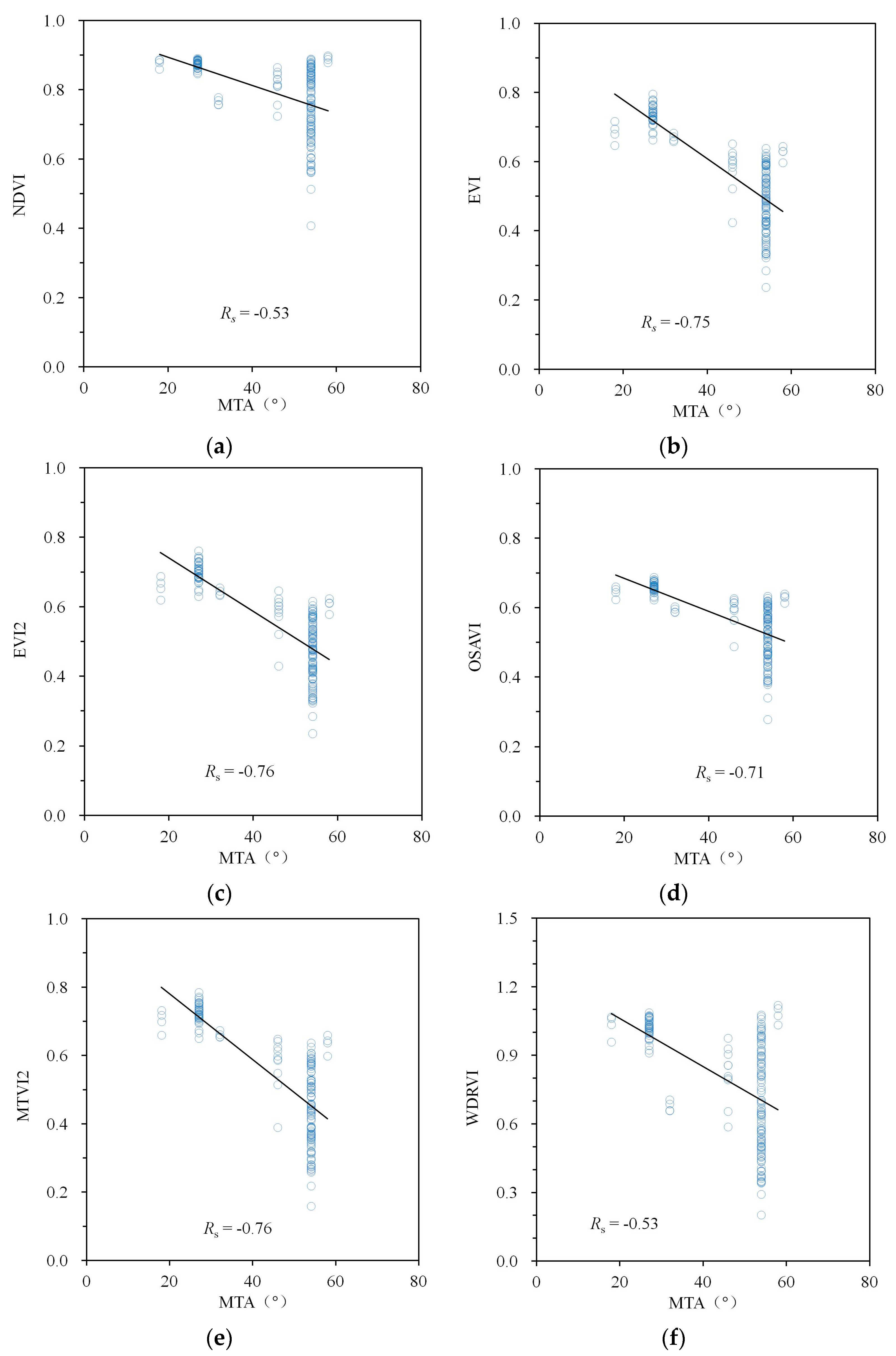
The correlations in the empirical dataset are presented graphically in Figure 3, Figure 4 and Figure 5. The species-specific MTA values cause the clustering of points into vertical stripes in these figures. The length of each stripe depends on the variation of a VI on parameters other than MTA. The variation of these parameters in the measured dataset is provided in Table 1 in the reference [20]. Despite considerable variation, the strong effect of MTA on EVI, EVI2, OSAVI and MTVI2 is clear from Figure 3b–e. For the other indices (Figure 3a,f) was lower (= −0.53) and the index values at MTA = 54° and MTA = 58° (wheat and oat, respectively) could be as high as for MTA = 18° and MTA = 27° (lupin and faba bean, respectively).
The correlation between the VIs and LAI were all positive (Figure 4). No obvious saturation at high LAI values (LAI > 3) was visible for any of the indices used in this study. However, the point clouds were divided into two subclouds with a small set of measurements with LAI = 2–3 (corresponding to faba bean and lupin, the two non-cereal crops with the lowest recorded MTAs) with VI values higher than the rest of the data.
The large values between the VIs and Fcover in Table 2 are accompanied by the close to linear point clouds with little scatter in Figure 5. Especially the VIs with the largest values (EVI, EVI2, OSAVI, MTVI2) are also characterized by the smallest scatter; however, the performance differences between the indices are small. A small non-linearity with Fcover can be visually detected for EVI, EVI2 and MTVI2 (Figure 5b–e), but not for OSAVI (Figure 5d).
4. Discussion
Clearly, the observed correlation with the leaf inclination angle in the field crop canopy (quantified by MTA) cannot be ignored when estimating other canopy biophysical parameters. Although it is possible that the spectral effect is caused by some other parameter strongly correlated with MTA, no other parameter has been identified in earlier modeling studies [29]. Thus far, the influence of LAD on VIs has not been adequately investigated with empirical data. In this study, we attempted to bridge this gap for six commonly used multispectral VIs characterizing canopy greenness.
The field-measured set of vegetation parameters covers a wide range of values covering a large majority of natural variations in both LAI and MTA. This allowed us to use a simple comparison of correlation coefficients, which depend on the level of variation included in each of the studied variables. Since the measured MTA and LAI ranges are representative of their natural variation, a comparison of the values of tells us about the role of each vegetation parameter in determining the studied VIs.
According to both PROSAIL model simulations and empirical data, all studied VIs depended on MTA with NDVI being the least affected. This supports the findings of previous studies by Liu et al. [33]. WDRVI is a nonlinear transformation of NDVI performed identically with NDVI when measured with Spearman’s R, however, the more common Pearson’s -value was slightly higher for WDRVI (0.25 and 0.30 for measured NDVI and WDRVI, respectively). NDVI and WDRVI were also the two indices with the strongest correlations with LAI in both the modeled and measured data (Table 2). However, the relatively strong (compared with other indices studied here) correlation between LAI and NDVI is compromised by the well-known saturation of the VI’s sensitivity to LAI evident in the variation of the distance between the lines in Figure 1a. The same non-linearity is present in WDRVI (Figure 1f).
EVI, EVI2 and MTVI2 were designed to be more sensitive to the variations inside the canopy by minimizing background influence, and working at large LAI values without saturation. In our measured dataset, the indices saturate less, with the lines in Figure 2b–e nearly parallel and more closely equidistant. Unfortunately, these VIs were more strongly correlated with MTA () than NDVI and WDRVI. The specific strength of the correlation between MTA and NDVI and WDRVI may somewhat depend on the spectral properties of soil. Using the sample curves in Figure 1b, a narrow-leafed lupin (MTA = 18°) canopy with LAI = 1 would have EVI ≈ 0.5. A similar EVI value is produced by an oat (MTA = 58°) canopy of LAI = 4. Our results demonstrate empirically that it is very difficult to quantify LAI using remotely sensed VIs when the MTA is unknown [49].
EVI and EVI2 are widely used for tracing the dynamics of vegetation gross primary production (GPP) and phenology inter- or inner-annually [50,51,52,53]. As MTA had a stronger effect on these VIs than LAI, caution should be used when applying them to estimate LAI across structurally potentially different canopies, e.g., seasonality studies or application over multiple crop species. Depending on cover type and LAI values, it may be more optimal to use NDVI or WDRVI, which produced relatively high with LAI in both model simulations and empirical data: the between the LAI and NDVI was 0.71 and 0.58 in simulated and measured data, respectively. This also agrees quantitatively with the previous finding by Colombo et al. [54] of for data pooled over five vegetation types (soybean, corn, vineyards, poplar plantation and deciduous forest).
In our study, the correlation between Fcover and WDRVI was the strongest with the values close to the value of 0.96 reported by Gitelson [55] in the simulated dataset. They also proposed the following equation for calculating Fcover from remote sensing data:
(Equation (2) in [55]). The proposed equation was more accurate for empirical (RMSE = 0.22, bias of mean = 0.18) than model-simulated (RMSE = 0.38, bias of mean = 0.37) data with some overestimation in both datasets.
For measured data, the best-performing indexes for estimating Fcover were EVI2 and MTVI2, with . In agreement with previous studies, we found that a new independent variable Fcover, a nonlinear combination of LAI and MTA, is the key driver of variation in the commonly used VIs. Hence, all the VIs studied here can be efficiently used to predict this structural parameter. The slightly better performance of EVI2 and MTVI2 can be attributed to the capability of the Spearman’s R to ignore the nonlinearity with Fcover. When the more traditional Pearson’s R is used (despite the non-normality of the data), the index most strongly correlated with Fcover is OSAVI () with a marginal difference to EVI2 and MTVI2 (. Similarly to this study, however, some nonlinearity and dependence on illumination conditions is expected [56] under varying conditions.
The results corroborate earlier findings, especially those by Liu et al. [33] and Gitelson [55]. As we have demonstrated empirically, even for homogeneous crop canopies, NDVI or its more sophisticated counterparts, EVI or EVI2, depend not only on LAI, but also on the second structural parameter, MTA. Furthermore, the dependence of the most widely used VIs on MTA can be stronger than on LAI with the actual effects of the two canopy parameters depending on their actual range of variation. Therefore, in order to map LAI from multispectral data, effective methods need to be developed to remotely measure leaf angles. This can be achieved, for example, using canopy reflectance in the red edge [22]. Although Earth observation data in this spectral region is scarce, it is covered by some systems, most notably Sentinel 2. We hope that future investigations into the application of this sensor into MTA estimations will improve the mapping of MTA, and thus also LAI.
5. Conclusions
The results of this study reveal that the test six common multispectral vegetation indices showed strong correlations with MTA, especially for EVI, EVI2 and MTVI2, with for both PROSAIL simulations and field-measured data. All studied VIs were proxies for the fractional canopy cover determined by two key elementary canopy parameters (leaf area index and leaf mean tilt angle). For the studied crops, EVI2 and MTVI2 were the best indicator for Fcover with for measured data and for model simulations.
Supplementary Materials
The following are available online at www.mdpi.com/2072-4292/9/10/994/s1.
Acknowledgments
The research was funded by Natural Science Foundation of Jiangsu Province (Grants No. BK20170950), Scientific Research Start-up Funds of NUIST (Grants No. 2016R27) and Academy of Finland project 266152. The SunScan measurement data was kindly provided by Priit Tammeorg, Clara Lizarazo Torres, Piia Kekkonen, F.L. Stoddard and Pirjo Mäkelä (Department of Agricultural Sciences, University of Helsinki).
Author Contributions
X.Z. and M.M. conceived and designed the experiments, analyzed the data and wrote the manuscript.
Conflicts of Interest
The authors declare no conflict of interest.
References
- Kimes, D.S. Effects of vegetation canopy structure on remotely sensed canopy temperature. Remote Sens. Environ. 1980, 10, 165–174. [Google Scholar] [CrossRef]
- Sassenrath-Cole, G.F. Dependence of canopy light distribution on leaf and canopy structure for two cotton (gossypium) species. Agric. For. Meteorol. 1995, 77, 55–72. [Google Scholar] [CrossRef]
- Tappeiner, U.; Cernusca, A. Model simulation of spatial distribution of photosynthesis in structurally differing plant communities in the Central Caucasus. Ecol. Model. 1998, 24, 272–279. [Google Scholar] [CrossRef]
- Gamon, J.A.; Field, C.B.; Goulden, M.L.; Griffin, K.L.; Hartley, A.E.; Joel, G.; Peñuelas, J.; Valentini, R. Relationships between NDVI, canopy structure, and photosynthesis in three Californian vegetation types. Ecol. Appl. 1995, 5, 28–41. [Google Scholar] [CrossRef]
- Running, S.W.; Baldocchi, D.D.; Turner, D.P.; Gower, S.T.; Bakwin, P.S.; Hibbard, K.A. A global terrestrial monitoring network integrating tower fluxes, flask sampling, ecosystem modeling and EOS satellite data. Remote Sens. Environ. 1999, 70, 108–127. [Google Scholar] [CrossRef]
- Chen, J.M.; Cihlar, J. Retrieving leaf area index of boreal conifer forests using landsat TM images. Remote Sens. Environ. 1996, 55, 153–162. [Google Scholar] [CrossRef]
- Koetz, B.; Baret, F.; Poilve, H.; Hill, J. Use of coupled canopy structure dynamic and radiative transfer models to estimate biophysical canopy characteristics. Remote Sens. Environ. 2005, 95, 115–124. [Google Scholar] [CrossRef]
- Ross, J. The Radiation Regime and Architecture of Plants Stands; Springer Science & Business Media: Medford, MA, USA, 1981. [Google Scholar]
- Myneni, R.B.; Williams, D.L. On the relationship between FPAR and NDVI. Remote Sens. Environ. 1994, 49, 200–211. [Google Scholar] [CrossRef]
- Moran, M.S.; Inoue, Y.; Barnes, E.M. Opportunities and Limitations for Image-Based Remote Sensing in Precision Crop Management. Remote Sens. Environ. 1997, 61, 319–346. [Google Scholar] [CrossRef]
- Le Maire, G.; François, C.; Soudani, K.; Berveiller, D.; Pontailler, J.Y.; Bréda, N. Calibration and validation of hyperspectral indices for the estimation of broadleaved forest leaf chlorophyll content, leaf mass per area, leaf area index and leaf canopy biomass. Remote Sens. Environ. 2008, 112, 3846–3864. [Google Scholar] [CrossRef]
- An, N.; Goldsby, A.L.; Price, K.P.; Bremer, D.J. Using hyperspectral radiometry to predict the green leaf area index of turfgrass. Int. J. Remote Sens. 2015, 36, 1470–1483. [Google Scholar] [CrossRef]
- Campbell, G.S.; Norman, J.M. An Introduction to Environmental Biophysics; Springer: New York, NY, USA, 1998. [Google Scholar]
- Welles, J.M.; Norman, J.M. Instrument for indirect measurement of canopy architecture. Agron. J. 1991, 83, 818–825. [Google Scholar] [CrossRef]
- Hosoi, F.; Omasa, K. Estimating vertical plant area density profile and growth parameters of a wheat canopy at different growth stages using three dimensional portable lidar imaging. ISPRS J. Photogramm. Remote Sens. 2009, 64, 151–158. [Google Scholar] [CrossRef]
- Paulus, S.; Schumann, H.; Kuhlmann, H.; Léon, J. High-precision laser scanning system for capturing 3D plant architecture and analysing growth of cereal plants. Biosyst. Eng. 2014, 121, 1–11. [Google Scholar] [CrossRef]
- Ryu, Y.; Sonnentag, O.; Nilson, T.; Vargas, R.; Kobayashi, H.; Wenk, R.; Baldocchi, D.D. How to quantify tree leaf area index in a heterogeneous savanna ecosystem: A multi-instrument and multi-model approach. Agric. For. Meteorol. 2010, 150, 63–76. [Google Scholar] [CrossRef]
- Pisek, J.; Ryu, Y.; Alikas, K. Estimating leaf inclination and G-function from leveled digital camera photography in broadleaf canopies. Trees 2011, 25, 919–924. [Google Scholar] [CrossRef]
- Pisek, J.; Sonnentag, O.; Richardson, A.D.; Mõttus, M. Is the spherical leaf inclination angle distribution a valid assumption for temperate and boreal broadleaf tree species? Agric. For. Meteorol. 2013, 169, 186–194. [Google Scholar] [CrossRef]
- Zou, X.; Mõttus, M.; Tammeorg, P.; Torres, C.L.; Takala, T.; Pisek, J.; Mäkelä, P.; Stoddard, F.L.; Pellikka, P. Photographic measurement of leaf angles in field crops. Agric. For. Meteorol. 2014, 184, 137–146. [Google Scholar] [CrossRef]
- Jacquemoud, S.; Verhoef, W.; Baret, F.; Bacour, C.; Zarco-Tejada, P.J.; Asner, G.P.; François, C.; Ustin, S.L. PROSPECT+ SAIL models: A review of use for vegetation characterization. Remote Sens. Environ. 2009, 113, S56–S66. [Google Scholar] [CrossRef]
- Zou, X.; Mõttus, M. Retrieving crop leaf tilt angle from imaging spectroscopy data. Agric. For. Meteorol. 2015, 205, 73–82. [Google Scholar] [CrossRef]
- Rouse, J.; Haas, H.; Schell, A.; Deering, W.; Harlan, C. Monitoring the Vernal Advancement of Retrogradation (Green Wave Effect) of Natural Vegetation; Type III, Final Report; NASA: Washington, DC, USA, 1974; pp. 1–371.
- Myneni, R.B.; Hall, F.G.; Sellers, P.J.; Marshak, A.L. The meaning of spectral vegetation indices. IEEE Trans. Geosci. Remote Sens. 1995, 33, 481–486. [Google Scholar] [CrossRef]
- Vicente-Serrano, S.M.; Camarero, J.J.; Olano, J.M.; Martín-Hernández, N.; Peña-Gallardo, M.; Tomás-Burguera, M.; Peña-Gallardo, M.; Tomás-Burguera, M.; Gazol, A.; Azorin-Molina, C.; et al. Diverse relationships between forest growth and the Normalized Difference Vegetation Index at a global scale. Remote Sens. Environ. 2016, 187, 14–29. [Google Scholar] [CrossRef]
- Skakun, S.; Franch, B.; Vermote, E.; Roger, J.C.; Becker-Reshef, I.; Justice, C.; Kussul, N. Early season large-area winter crop mapping using MODIS NDVI data, growing degree days information and a Gaussian mixture model. Remote Sens. Environ. 2017, 195, 244–258. [Google Scholar] [CrossRef]
- Huete, A.; Didan, K.; Miura, T.; Rodriguez, E.; Gao, X.; Ferreira, L. Overview of the radiometric and biophysical performance of the MODIS vegetation indices. Remote Sens. Environ. 2002, 83, 195–213. [Google Scholar] [CrossRef]
- Jiang, Z.; Huete, A.; Didan, K.; Miura, T. Development of a two-band enhanced vegetation index without a blue band. Remote Sens. Environ. 2008, 112, 3833–3845. [Google Scholar] [CrossRef]
- Rondeaux, G.; Steven, M.; Baret, F. Optimization of soil-adjusted vegetation indices. Remote Sens. Environ. 1996, 55, 95–107. [Google Scholar] [CrossRef]
- Haboudane, D.; Miller, J.; Pattery, E.; Zarco, P.; Strachan, B. Hyperspectral vegetation indices and novel algorithms for predicting green LAI of crop canopies: Modeling and validation in the context of precision agriculture. Remote Sens. Environ. 2004, 90, 337–352. [Google Scholar] [CrossRef]
- Gitelson, A.A. Wide Dynamic Range Vegetation Index for remote quantification of biophysical characteristics of vegetation. J. Plant Physiol. 2004, 161, 165–173. [Google Scholar] [CrossRef] [PubMed]
- Peng, Y.; Gitelson, A.A. Application of chlorophyll-related vegetation indices for remote estimation of maize productivity. Agric. For. Meteorol. 2011, 151, 1267–1276. [Google Scholar] [CrossRef]
- Liu, J.; Pattey, E.; Jégo, G. Assessment of vegetation indices for regional crop green LAI estimation from Landsat images over multiple growing seasons. Remote Sens. Environ. 2012, 123, 347–358. [Google Scholar] [CrossRef]
- ImageJ. Available online: http://rsb.info.nih.gov/ij/) (accessed on 15 September 2017).
- Weiss, M.; Baret, F.; Smith, G.J.; Jonckheere, I.; Coppin, P. Review of methods for in situ leaf area index (LAI) determination. Part II. Estimation of LAI, errors and sampling. Agric. For. Meteorol. 2004, 121, 37–53. [Google Scholar] [CrossRef]
- Campbell, G.S. Derivation of an angle density function for canopies with ellipsoidal leaf angle distributions. Agric. For. Meteorol. 1990, 49, 173–176. [Google Scholar] [CrossRef]
- Walthall, C.L.; Norman, J.M.; Welles, J.M.; Campbell, G.; Blad, B.L. Simple equation to approximate the bidirectional reflectance from vegetative canopies and bare soil surfaces. Appl. Opt. 1985, 24, 383–387. [Google Scholar] [CrossRef] [PubMed]
- Nilson, T.; Kuusk, A. A reflectance model for the homogenous plant canopy and its inversion. Remote Sens. Environ. 1989, 27, 157–167. [Google Scholar] [CrossRef]
- Feret, J.-B.; Francois, C.; Asner, G.P.; Gitelson, A.A.; Martin, R.E.; Bidel, L.P.R.; Ustin, S.L.; le Maire, G.; Jacquemoud, S. PROSPECT-4 and 5: Advances in the leaf optical properties model separating photosynthetic pigments. Remote Sens. Environ. 2008, 112, 3030–3043. [Google Scholar] [CrossRef]
- Verhoef, W. Light scattering by leaf layers with application to canopy reflectance modeling: The SAIL model. Remote Sens. Environ. 1984, 16, 125–141. [Google Scholar] [CrossRef]
- Kuusk, A. The hot spot effect in plant canopy reflectance. In Photon-Vegetation Interactions; Springer: Berlin, Germany, 1991; pp. 139–159. [Google Scholar]
- Campbell, G.S. Extinction coefficients for radiation in plant canopies calculated using an ellipsoidal inclination angle distribution. Agric. For. Meteorol. 1986, 36, 317–321. [Google Scholar] [CrossRef]
- Mäkelä, P.; Kleemola, J.; Jokinen, K.; Mantila, J.; Pehu, E.; Peltonen-Sainio, P. Growth response of pea and summer turnip rape to foliar application of glycinebetaine. Acta Agric. Scand. Sect. B Soil Plant Sci. 1997, 47, 168–175. [Google Scholar] [CrossRef]
- Dennett, M.D.; Ishag, K.H.M. Use of the expolinear growth model to analyze the growth of faba bean, Peas and lentils at three densities: Predictive use of the model. Ann. Bot. 1998, 82, 507–512. [Google Scholar] [CrossRef]
- Pinheiro, C.; Rodrigues, A.P.; de Carvalho, I.S.; Chaves, M.M.; Ricardo, C.P. Sugar metabolism in developing lupin seeds is affected by a short-term water deficit. J. Exp. Bot. 2005, 56, 2705–2712. [Google Scholar] [CrossRef] [PubMed]
- Vile, D.; Garnier, E.; Shipley, B.; Laurent, G.; Navas, M.L.; Roumet, C.; Lavorel, S.; Diaz, S.; Hodgson, J.G.; Lloret, F.; et al. Specific leaf area and dry matter content estimate thickness in laminar leaves. Ann. Bot. 2005, 96, 1129–1136. [Google Scholar] [CrossRef] [PubMed]
- Vermote, E.F.; Tanre, D.; Deuze, J.L.; Herman, M.; Morcrette, J.J. Second simulation of the satellite signal in the solar spectrum, 6S: An overview. IEEE Trans. Geosci. Remote Sens. 1997, 35, 675–686. [Google Scholar] [CrossRef]
- Hosgood, B.; Jacquemoud, S.; Andreoli, G.; Verdebout, J.; Pedrini, G.; Schmuck, G. Leaf Optical Properties Experiment 93 (Lopex93); Office for Official Publications of the European Communities: Brussels, Luxembourg, 1994. [Google Scholar]
- Baret, F.; Guyot, G. Potentials and limits of vegetation indices for LAI and APAR assessment. Remote Sens. Environ. 1991, 35, 161–173. [Google Scholar] [CrossRef]
- Gitelson, A.A.; Vina, A.; Verma, S.B.; Rundquist, D.C.; Arkebauer, T.J.; Keydan, G.; Leavitt, B.; Ciganda, V.; Burba, G.G.; Suyker, A.E. Relationship between gross primary production and chlorophyll content in crops: Implications for the synoptic monitoring of vegetation productivity. J. Geophys. Res. 2006, 111. [Google Scholar] [CrossRef]
- Zhang, X.; Friedl, M.A.; Schaaf, C.B. Global vegetation phenology from Moderate Resolution Imaging Spectroradiometer (MODIS): Evaluation of global patterns and comparison with in situ measurements. J. Geophys. Res. 2006, 111. [Google Scholar] [CrossRef]
- Sims, D.A.; Rahman, A.F.; Cordova, V.D.; El-Masri, B.Z.; Baldocchi, D.D.; Bolstad, P.V.; Bolstad, P.V.; Flanagan, L.B.; Goldstein, A.H.; Hollinger, D.Y.; et al. A new model of gross primary productivity for North American ecosystems based solely on the enhanced vegetation index and land surface temperature from MODIS. Remote Sens. Environ. 2008, 112, 1633–1646. [Google Scholar] [CrossRef]
- Wu, C.; Niu, Z.; Gao, S. Gross primary production estimation from MODIS data with vegetation index and photosynthetically active radiation in maize. J. Geophys. Res. 2010, 115. [Google Scholar] [CrossRef]
- Colombo, R.; Bellingeri, D.; Fasolini, D.; Marino, C.M. Retrieval of leaf area index in different vegetation types using high resolution satellite data. Remote Sens. Environ. 2003, 86, 120–131. [Google Scholar] [CrossRef]
- Gitelson, A.A. Remote estimation of crop fractional vegetation cover: The use of noise equivalent as an indicator of performance of vegetation indices. Int. J. Remote Sens. 2013, 34, 1–13. [Google Scholar] [CrossRef]
- Steven, M.D. The sensitivity of the OSAVI vegetation index to observational parameters. Remote Sens. Environ. 1998, 63, 49–60. [Google Scholar] [CrossRef]
Figure 1.
The soil reflectance used for PROSAIL simulations.

Figure 2.
Relationship between MTA and VIs at different LAI values (low: LAI = 1, medium: LAI = 3 and high: LAI = 5) for (a) NDVI, (b) EVI, (c) EVI2, (d) OSAVI, (e) MTVI2, (f) WDRVI.
Figure 2.
Relationship between MTA and VIs at different LAI values (low: LAI = 1, medium: LAI = 3 and high: LAI = 5) for (a) NDVI, (b) EVI, (c) EVI2, (d) OSAVI, (e) MTVI2, (f) WDRVI.
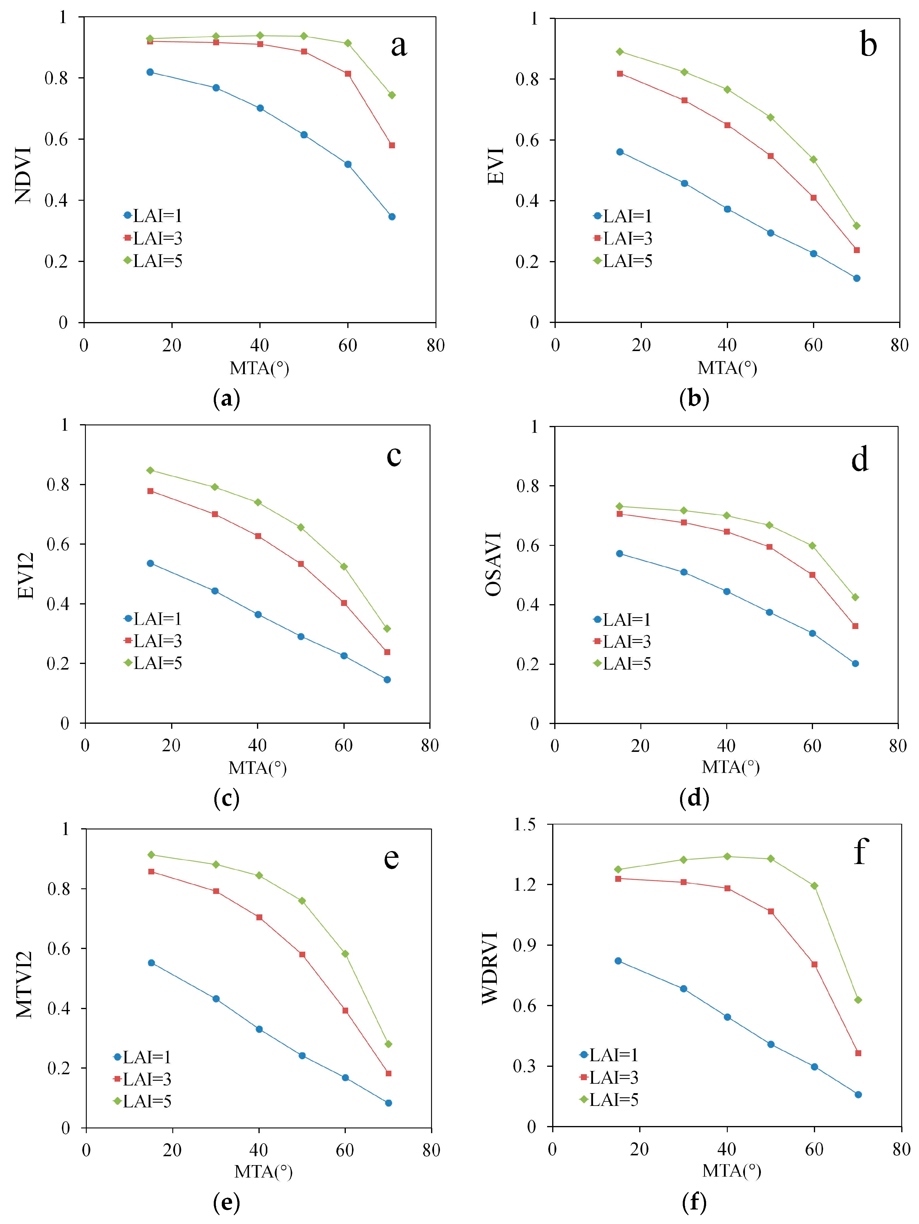
Figure 3.
Empirical relationships between MTA and VIs calculated from Spearman’s correlation coefficient Rs: (a) NDVI, (b) EVI, (c) EVI2, (d) OSAVI, (e) MTVI2, (f) WDRVI. A simple trend line calculated from linear regression was added to visualize the trend of the variation.
Figure 3.
Empirical relationships between MTA and VIs calculated from Spearman’s correlation coefficient Rs: (a) NDVI, (b) EVI, (c) EVI2, (d) OSAVI, (e) MTVI2, (f) WDRVI. A simple trend line calculated from linear regression was added to visualize the trend of the variation.

Figure 4.
Empirical relationships between LAI and VIs calculated from Spearman’s correlation coefficient Rs: (a) NDVI, (b) EVI, (c) EVI2, (d) OSAVI, (e) MTVI2, (f) WDRVI. A simple trend line calculated from linear regression was added to visualize the trend of the variation.
Figure 4.
Empirical relationships between LAI and VIs calculated from Spearman’s correlation coefficient Rs: (a) NDVI, (b) EVI, (c) EVI2, (d) OSAVI, (e) MTVI2, (f) WDRVI. A simple trend line calculated from linear regression was added to visualize the trend of the variation.
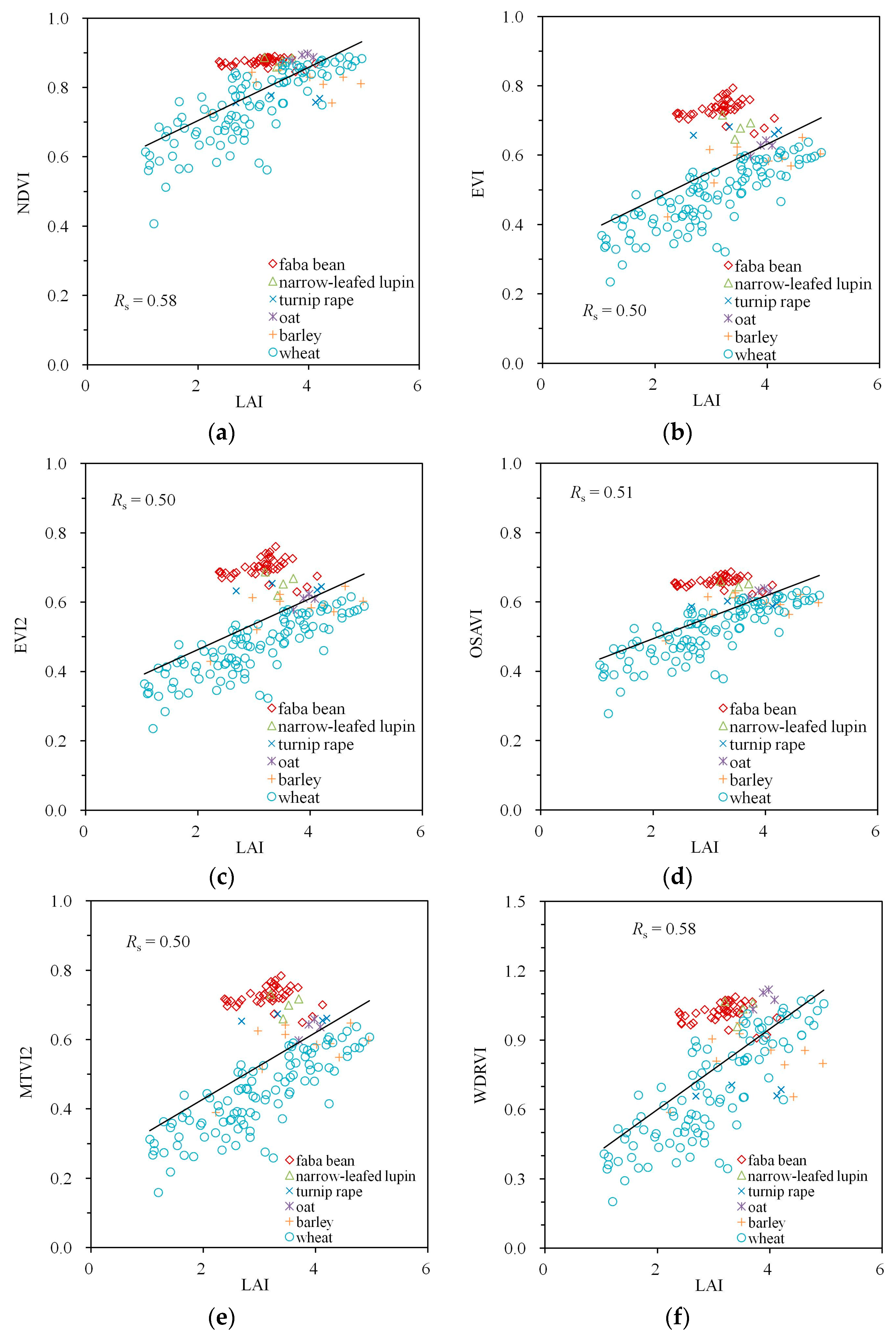
Figure 5.
Empirical relationships between Fcover and VIs calculated from Spearman’s correlation coefficient Rs: (a) NDVI, (b) EVI, (c) EVI2, (d) OSAVI, (e) MTVI2, (f) WDRVI. A simple trend line calculated from linear regression was added to visualize the trend of the variation.
Figure 5.
Empirical relationships between Fcover and VIs calculated from Spearman’s correlation coefficient Rs: (a) NDVI, (b) EVI, (c) EVI2, (d) OSAVI, (e) MTVI2, (f) WDRVI. A simple trend line calculated from linear regression was added to visualize the trend of the variation.

Table 1.
Vegetation indices used in this study.
| Index | Formula | References |
|---|---|---|
| NDVI | [23] | |
| EVI | [27] | |
| EVI2 | [28] | |
| OSAVI | [29] | |
| MTVI2 | [30] | |
| WDRVI | [31,32] |
Table 2.
Spearman’s correlation coefficient () between spectral indices and canopy structural variables.
Table 2.
Spearman’s correlation coefficient () between spectral indices and canopy structural variables.
| Spectral Index | Simulations | Measurements | ||||
|---|---|---|---|---|---|---|
| MTA | LAI | Fcover | MTA | LAI | Fcover | |
| NDVI | −0.59 | 0.71 | 0.96 | −0.53 | 0.58 | 0.78 |
| EVI | −0.83 | 0.52 | 0.93 | −0.75 | 0.50 | 0.87 |
| EVI2 | −0.82 | 0.54 | 0.93 | −0.76 | 0.50 | 0.88 |
| OSAVI | −0.78 | 0.58 | 0.95 | −0.71 | 0.51 | 0.86 |
| MTVI2 | −0.81 | 0.54 | 0.93 | −0.76 | 0.50 | 0.88 |
| WDRVI | −0.59 | 0.71 | 0.96 | −0.53 | 0.58 | 0.78 |
© 2017 by the authors. Licensee MDPI, Basel, Switzerland. This article is an open access article distributed under the terms and conditions of the Creative Commons Attribution (CC BY) license (http://creativecommons.org/licenses/by/4.0/).
Share and Cite
MDPI and ACS Style
Zou, X.; Mõttus, M. Sensitivity of Common Vegetation Indices to the Canopy Structure of Field Crops. Remote Sens. 2017, 9, 994. https://doi.org/10.3390/rs9100994
AMA Style
Zou X, Mõttus M. Sensitivity of Common Vegetation Indices to the Canopy Structure of Field Crops. Remote Sensing. 2017; 9(10):994. https://doi.org/10.3390/rs9100994
Chicago/Turabian StyleZou, Xiaochen, and Matti Mõttus. 2017. "Sensitivity of Common Vegetation Indices to the Canopy Structure of Field Crops" Remote Sensing 9, no. 10: 994. https://doi.org/10.3390/rs9100994
Note that from the first issue of 2016, this journal uses article numbers instead of page numbers. See further details here.