Hashing Based Hierarchical Feature Representation for Hyperspectral Imagery Classification

1
Image Processing Center, School of Astronautics, Beihang University, Beijing 100191, China
2
Beijing Key Laboratory of Digital Media, Beihang University, Beijing 100191, China
3
State Key Laboratory of Virtual Reality Technology and Systems, School of Astronautics, Beihang University, Beijing 100191, China
4
Mathematics Department, Mellon College of Science, Carnegie Mellon University, Pittsburgh, PA 15213, USA
*
Author to whom correspondence should be addressed.
Remote Sens. 2017, 9(11), 1094; https://doi.org/10.3390/rs9111094
Submission received: 24 September 2017
/
Revised: 19 October 2017
/
Accepted: 24 October 2017
/
Published: 27 October 2017
(This article belongs to the Special Issue Hyperspectral Imaging and Applications)
Abstract
:Integrating spectral and spatial information is proved effective in improving the accuracy of hyperspectral imagery classification. In recent studies, two kinds of approaches are widely investigated: (1) developing a multiple feature fusion (MFF) strategy; and (2) designing a powerful spectral-spatial feature extraction (FE) algorithm. In this paper, we combine the advantages of MFF and FE, and propose an ensemble based feature representation method for hyperspectral imagery classification, which aims at generating a hierarchical feature representation for the original hyperspectral data. The proposed method is composed of three cascaded layers: firstly, multiple features, including local, global and spectral, are extracted from the hyperspectral data. Next, a new hashing based feature representation method is proposed and conducted on the features obtained in the first layer. Finally, a simple but efficient extreme learning machine classifier is employed to get the classification results. To some extent, the proposed method is a combination of MFF and FE: instead of feature fusion or single feature extraction, we use an ensemble strategy to provide a hierarchical feature representation for the hyperspectral data. In the experiments, we select two popular and one challenging hyperspectral data sets for evaluation, and six recently proposed methods are compared. The proposed method achieves respectively 89.55%, 99.36% and 77.90% overall accuracies in the three data sets with 20 training samples per class. The results prove that the performance of the proposed method is superior to some MFF and FE based ones.

1. Introduction
Hyperspectral sensors can provide images with hundreds of continuous spectral bands, which has attracted a number of applications such as environmental monitoring and mineral prospecting [1,2,3,4]. Among many surveys about hyperspectral imagery (HSI) analysis, land cover accurate classification is an important research topic. Supervised spectral classifiers are popular in the early research, including multinomial logistic regression [5], support vector machines (SVMs) [6,7,8] and sparse representation classifier [9].
During the last decade, a lot of endeavors have been devoted to extracting more representative features from original HSI data. It is widely recognized that joint spectral and spatial information can significantly improve the performance of HSI classification methods. Markov random field (MRF) is a powerful tool that is able to model the spatial relationship around pixels. In [10,11], MRF was combined with subspace multinomial logistic regression and Gaussian mixture model, respectively. In [12], MRF was used as a postprocessing to refine the classification maps obtained by SVM. Morphological profile (MP) is another powerful tool to utilize the spatial contextual information. In [13], Benediktsson et al. improved the original MP, and proposed the extended morphological profile (EMP) method for HSI classification. Motivated by the promising performance of EMP, two improved methods, extended attribute profile and extended multi-attribute profile, were proposed in [14].
Because a single kind of feature may not describe the integrated characteristics of HSI data, multiple feature fusion (MFF) were proposed and used to improve the performance of HSI classification models. MFF based methods can be roughly divided into four classes [15]: multiple kernel learning, band selection, subspace feature extraction and ensemble based methods. Li et al. constructed a series of generalized composite kernels where no weight parameters were required [16]. Gu et al. employed multiple kernel learning to combine different spectral-spatial features [17,18,19]. Band selection methods try to find the most discriminative hyperspectral channels while preserving their physical meanings. In [20], discriminative sparse multimodal learning based method was proposed for multiple feature selection. In [21], spectral and spatial information are utilized simultaneously to select the representative bands. Different from band selection, subspace methods refer to transforming the original multiple features to a new low-dimension sub-feature space. Zhang et al. introduced a patch alignment and a modified stochastic neighbor embedding based methods for feature fusion [22,23]. In [24], a low-rank representation based feature extraction method was proposed for HSI classification, where locally spatial similarity and spectral space structure were combined. In [15], Zhong et al. conducted dimension reduction on multiple features by hashing methods. Ensemble learning is another typical feature fusion method. Ensemble learning methods aim at achieving better generalization capacity by integrating different features or individual learners [25]. SVM [26,27] and random forest [28,29,30] based HSI classification methods were proposed in recent studies. In [31], Chen et al. improved the classification accuracy by stacked generalization of magnitude and shape feature spaces. In [32], Pan et al. combined spatial relationships in different scales via a weighted voting strategy. In addition, feature fusion methods using different data sources have also been investigated [33,34].
Recently, deep learning based methods have attracted great interest in HSI classification, e.g., [35,36,37,38,39,40]. The basic idea of these methods is to extract the “deep” feature from the original HSI data, thus hierarchical network models are designed. This idea is promising and encouraging. In some natural scene image classification tasks, deep learning methods have achieved even better results than human level [41]. In [35], the deep learning method was firstly used in HSI classification, where a stacked autoencoder was adopted. Subsequently, deep belief networks [42], convolutional neural networks [39,43,44] and recurrent neural networks [38] were investigated. In order to improve the computational efficiency, some simplified deep learning models were developed [36,37]. Most of these methods have also considered the spatial relationship via 3D networks or neighborhood information. However, the performance of deep learning methods is heavily dependant on abundant training samples that are difficult to acquire from HSI data. Compared with traditional methods, deep learning methods usually require more labeled samples. For example, in [35,36], about half of all the labeled pixels were used for training. Although deep features could really improve the classification accuracy, more research is required on finding a new way out of deep learning to extract hierarchical features.
Inspired by the ideas of MFF and deep learning, in this paper, we propose a novel hashing based hierarchical feature () extraction method for HSI classification. The motivations of come from two aspects: (1) low-level features such as spectral variations, local texture and global texture information, should be combined to produce a comprehensive feature set. This feature set could serve as inputs of the next layer; (2) based on the obtained feature set, a further feature extraction process should be followed, so as to generate a hierarchical feature. This hierarchical feature should present better performance than every single feature. Different from traditional MFF based methods, is not a simple combination or voting of multiple features. Instead, attempts to construct more representative feature descriptor from the already extracted feature set.
Based on the two motivations, we propose a cascaded feature extraction framework with two major processes: the generation of spectral-spatial feature set and hashing based hierarchical feature extraction. In the first process, we construct a feature set which is composed of spectral variations, local and global textures. In this paper, we use rolling guidance filtering (RGF) [45], local binary pattern (LBP) [46] and global Gabor filtering [47] to form the multiple features. Although many recent works have demonstrated that there is information redundant in some popular HSI data sets [48,49,50], it may be not appropriate to conclude that information redundant exists in all the HSI data. Therefore, different from traditional feature fusion based methods, in this paper, we do not conduct dimension reduction so as to better preserve the distinctive classification information. All these features are collected to a feature set. In the second process, we design a hashing histograms based feature extraction strategy to give a more representative description for the HSI data. To avoid complex computation, the feature set is separated into several groups. The hashing histogram features in all the groups are concatenated as the final feature expression. It is worth noting that is actually an ensemble based method, rather than deep learning based.
At last, an extreme learning machine (ELM) classifier [51] is used to determine the label of each pixel. The most important reason of using ELM is to improve the computing speed. Usually, feature fusion methods will generate relatively high-dimensional features, and this is more apparent in since dimension reduction is not adopted. ELM has a simple structure, and it can be trained very fast because of its random weights generation in inputs and least squares solution in outputs. Furthermore, some research has proven that ELM is effective for HSI classification [46,52,53]. We compare the effectiveness and efficiency of ELM and several other classifiers in the experiments’ part.
The major contribution of this paper is that a hashing based hierarchical feature ensemble method is developed. The ensemble strategy proposed in could provide a new way to utilize multiple features.
2. Based Classification
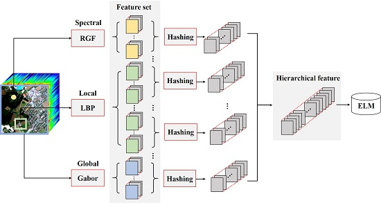
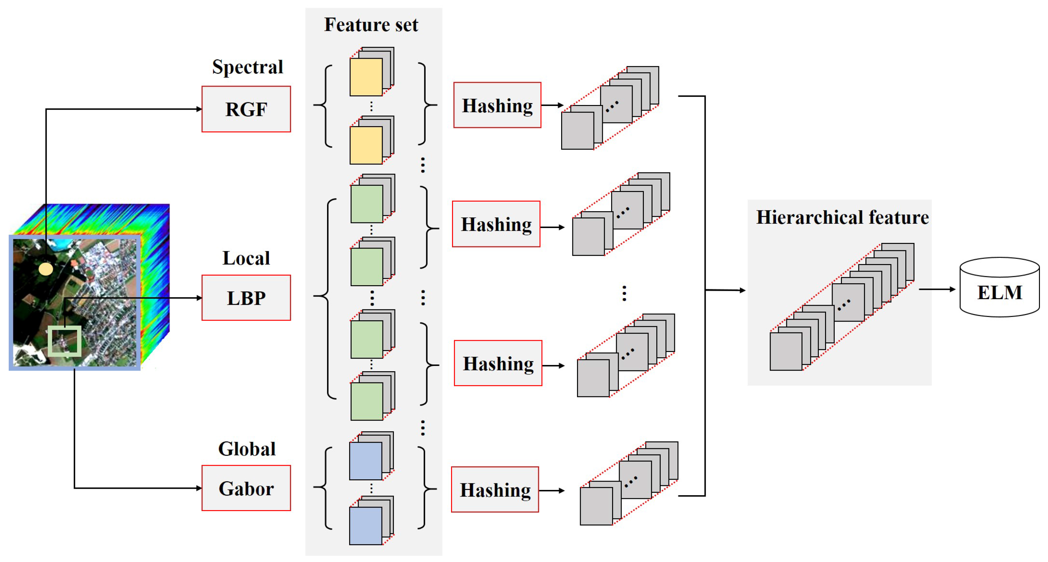
The proposed based HSI classification method can be divided into three steps: (1) multiple features extraction; (2) hashing based hierarchical feature representation and (3) ELM based classification. The flowchart of the proposed method is shown in Figure 1.
2.1. Multiple Features Extraction
Research has demonstrated that spectral-spatial joint information could significantly contribute to the performance of HSI classification methods. However, it is hard to judge which feature extraction approach performs best. Actually, each single feature has its unique emphasis. In this paper, we select three disparate features that reflect different characteristics of HSI data to construct a feature set, namely, RGF (for spectra), LBP (for local texture) and Gabor (for global texture). It is worth noting that each feature will generate one or several sub-feature sets. Take Gabor feature for example. Suppose that four wavelengths and four orientations are used. Then, for each pixel, there will be 16 sub-features. If we set eight as the number of features in a sub-feature set, two groups of sub-feature sets could be obtained. The following hierarchical feature representation operation is conducted on these subsets. Using the whole feature set directly for hierarchical feature representation is not appropriate because different types of features are heterogeneous.
2.1.1. RGF
Although the raw pixel spectral vectors could directly be used for training and classification, they do not perform well. Moreover, since we need sub-feature sets from spectral features, we must extend the pixels spectra to a group of features. Motivated by the effectiveness of RGF and its improvement in HSI classification [37], in this paper, we use RGF to obtain the sub-feature set using spectral information.
Let denote filtering result for the pth band of an hyperspectral image, we conduct guided filtering [54] by
where is a guidance image, i is one of a pixel in , is a window around pixel i, k is one of a pixel in , and and are coefficients to be estimated. Usually, is the first principal component of HSI data. Please note that only works as the guidance image, and it will not reduce the dimensionality of the filtered results. Then, minimize the following energy function:
where is the input HSI data, and is a hyper-parameter. Equation (2) can be solved directly by linear ridge regression [55]:
where and denote the mean value and standard variance of in , is the mean value of in , and is the number of pixels in .
Equation (1) is the optimization problem in guidance filtering, and a and b are the values need to be optimized. Equation (2) is the optimization object function, and Equation (3) is the solution. Rolling operation refers to replace by and conduct Equations (1) and (2) repeatedly. In each rolling, we can obtain a new HSI data. Therefore, using RGF we are able to generate a series of features based on the original spectral vectors. Because RGF mainly reflects the spectral characteristics of HSI data, these features can be considered as spectral sub-feature sets.
2.1.2. LBP
In HSI data, the spatial contextual information could be described by the local texture around each pixel. LBP feature is a popular texture operator that has been investigated in [46]. The LBP map for can be obtained by
where is the number of pixels in the window , and is a Heaviside step function with 1 for positive entries and 0, otherwise. In the LBP map, we can get a vector for each by counting its histogram. This vector is the new feature representation for pixel i. In this paper, uniform LBP is used. If using 8-neighbor for uniform LBP, 59 bins will be obtained totally, i.e., there are 59 sub-feature sets available based on LBP.
2.1.3. Gabor Filters
Besides local texture features, recent literature has reported that global spatial features of HSI data will also contribute to the classification accuracy, e.g., Gabor filter [47,56,57]. Suppose is a pixel coordinate at , then the output of an Gabor filter can be expressed by
where
, and are hyper-parameters in Gabor filter, is the wavelength of the sinusoidal function, and represents the orientation of the filter. Selecting different and , the original HSI data can be transformed into many sub-feature sets.
Based on the RGF, LBP and Gabor filters, we can construct a new feature set containing many subsets. Note that the dimensionality of features in the obtained set is the same with that of the original HSI data. Traditional feature fusion based methods usually directly stack these features, or use a weighted voting strategy. In this paper, we try to extract hierarchical features from HSI data, and this feature set is used as the input of the next hierarchy.
2.2. Hashing Based Hierarchical Feature Representation
The major motivation of the proposed hashing based method is that extracting very sparse features by increasing the feature dimensionality. For the obtained feature set, we first divide it into several subsets with the same number of features. Suppose N is the number of features in a single subset, and L is the dimensionality of features. Then, the illustration of hierarchical feature representation for this subset can be exhibited by Figure 2. Generally, the hashing based hierarchical feature representation method for a subset mainly includes three steps.
2.2.1. Step 1
For pixel i in position , we can obtain N features. Let denote the nth sub-feature, we conduct locality-sensitive hashing (LSH) on , i.e.,
where is a random matrix with zero-mean normal distribution, and is a binary vector. Integrating all the N vectors, we get .
2.2.2. Step 2
2.2.3. Step 3
Use a sliding window with size to scan , and then collect all the patches. Calculate the histogram features in all the patches (with bins), and concatenate them into a single vector , where denotes the mth sub-feature set, M is the number of sub-feature set, and if the step size of sliding window is set as 1. At last, the final hierarchical feature for pixel i is determined by
Obviously, increasing the step size of sliding window could reduce the dimensionality of the obtained features. Usually, 50% overlapping between patches is appropriate. Size of sliding window also has some influence on the results. Theoretically, smaller w could enhance the sparsity of the obtained features, but lead to very high dimensionality. In order to balance the sparsity and computational cost of computer memory, we set the window size as .
could be considered as a hierarchical representation for the original HSI data. According to our empirical experience, we do not recommend dimension reduction on because it may lead to loss of distinctive information. Instead, to reduce the computational cost and avoid overfitting, we use a very simple classifier, ELM, to determine the final classification results.
2.3. ELM Based Classification
ELM [51] is a simple neural network with only three layers (input, hidden and output), which performs well in small-scale data sets. ELM has two leadings characteristics: (1) the input and hidden layers are connected randomly; and (2) the weights between hidden and output layers are learned by a least squares algorithm.
Let denote the training samples matrix, d is the dimension and is the number of training samples. In ELM, the weights between input and hidden layers are obtained randomly, denoted by , where is the number of nodes in the hidden layer. Then, the objective function of ELM can be described by
where is the weights matrix connecting hidden and output layer, is the bias vector in the hidden layer, is an activation function such as sigmoid function, C is the number of classes, and is the label matrix for all the training samples. Note that is the output of the hidden layer for sample . Because and are randomly assigned, the outputs of the hidden layer have been determined. Then, Equation (10) is actually equal to the following expression:
where is the outputs of the hidden layer. Obviously, Equation (11) can be solved by a simple least squares method, i.e., .
In , the final features are classified by ELM. Because the random matrix generation needs little time, the major computational cost lies in Equation (11). As long as we restrict the number of hidden nodes, the training operation could be very fast. In Algorithm 1, we provide a pseudocode for the based HSI classification method.
| Algorithm 1 The based HSI classification method |
| Input: HSI data, ground truth |
| Initialize: training set, testing set |
| Multiple Features Extraction |
| 1. RGF features based on Equations (1) and (2) |
| 2. LBP features based on Equations (4) |
| 3. Gabor features based on Equations (5) and (6) |
| 4. Feature set generation |
| Hashing based Hierarchical Features |
| 5. Separate the feature set into uniform subsets |
| 6. For 1: Number of subsets |
| Hierarchical feature extraction by Equations (7) and (8) |
| End for |
| 7. Final features generation by Equation (9) |
| ELM based Classification |
| 8. Train ELM by Equations (10) and (11) |
| 9. Classification by ELM |
| Output: Classification results |
3. Experiments and Discussion
3.1. Experimental Setups
In this section, experimental analysis about the based classification method are provided. is compared with six recently proposed methods, i.e., Gabor + ELM (GE) [47], LBP + Gabor + ELM (LGE) [46], RGF + Network (RVCANet) [37], RGF + Ensemble (HiFi) [32], and another two methods, edge-preserving filtering (EPF) [58] and intrinsic image (IIDF) [59] based methods. Among these methods, GE and LGE directly concatenate multiple features without further operations. Thus, they could be regarded as the baselines. RVCANet also tries to extract deep features from HSI data, but it adopts a deep network manner. HiFi is a multiple feature fusion method where the results are obtained by weighted voting. These methods have similar motivation as the proposed method, so we use them for comparison. All the methods are compared on two popular (Indian Pines, Kennedy Space Center (KSC) (Available online: http://www.ehu.eus/ccwintco/index.php?title=Hyperspectral_Remote_Sensing_Scenes)) and one challenging (GRSS_DFC_2014 [60,61]) data set. We run the above methods 50 times with randomly selected train and test samples, and the average accuracies and the corresponding standard deviations are reported. Overall accuracy (OA), average accuracy (AA) and kappa coefficient () are selected for evaluation [62]. For the three data sets, 20 pixels per class are used for training, and the rests for testing. Some classes (especially in Indian Pines data set) have a total of nearly 20 samples. In this case, we directly use half of them for training and the others for testing. In , we construct nine sub-feature sets (six for LBP, two for Gabor and one for RGF) with nine features per set, totally 81 features. Rolling times of RGF is set as 1–9 with , wavelength in Gabor is 16, orientation number is 18, and window size in LBP is 3 × 3. Under this setting, Indian Pines/KSC/GRSS_DFC_2014 could be represented by 225792/198144/92160 dimensional features, but only 1% around are non-zero. The hyper-parameters in ELM (linear kernel) is determined by five-fold cross validation. The regularization coefficient is chosen from a set {1, 10, 100, 1000}, and the hidden neuron number is chosen from {100, 200, ⋯, 2000}. According to the results of cross validation, 1000 and 100 are appropriate for the above two parameters.
3.2. Data Sets
- Indian Pines: This data is widely used in HSI classification, which was gathered by airborne visible/infrared imaging spectrometer (AVIRIS) in Northwestern Indiana. It covers the wavelengths ranges from 0.4 to 2.5 μm with 20 m spatial resolution. In total, pixels are included and 10,249 of them are labeled. The labeled pixels are classified into 16 classes. There are 200 bands available after removing the water absorption channels. A false color composite image (R-G-B=band 36-17-11) and the corresponding ground truth are shown in Figure 3a,b.
- KSC: It is acquired by AVIRIS over the Kennedy Space Center, Florida, on March, 1996. It has 18 m spatial resolution with pixels size and 10 nm spectral resolution with center wavelengths from 400 to 2500 nm. In addition, 176 bands could be used for analysis after removing water absorption and low SNR bands. There are 5211 labeled pixels available that are divided into 16 classes. A false color composite image (R-G-B=band 28-9-10) and the corresponding ground truth are shown in Figure 3c,d.
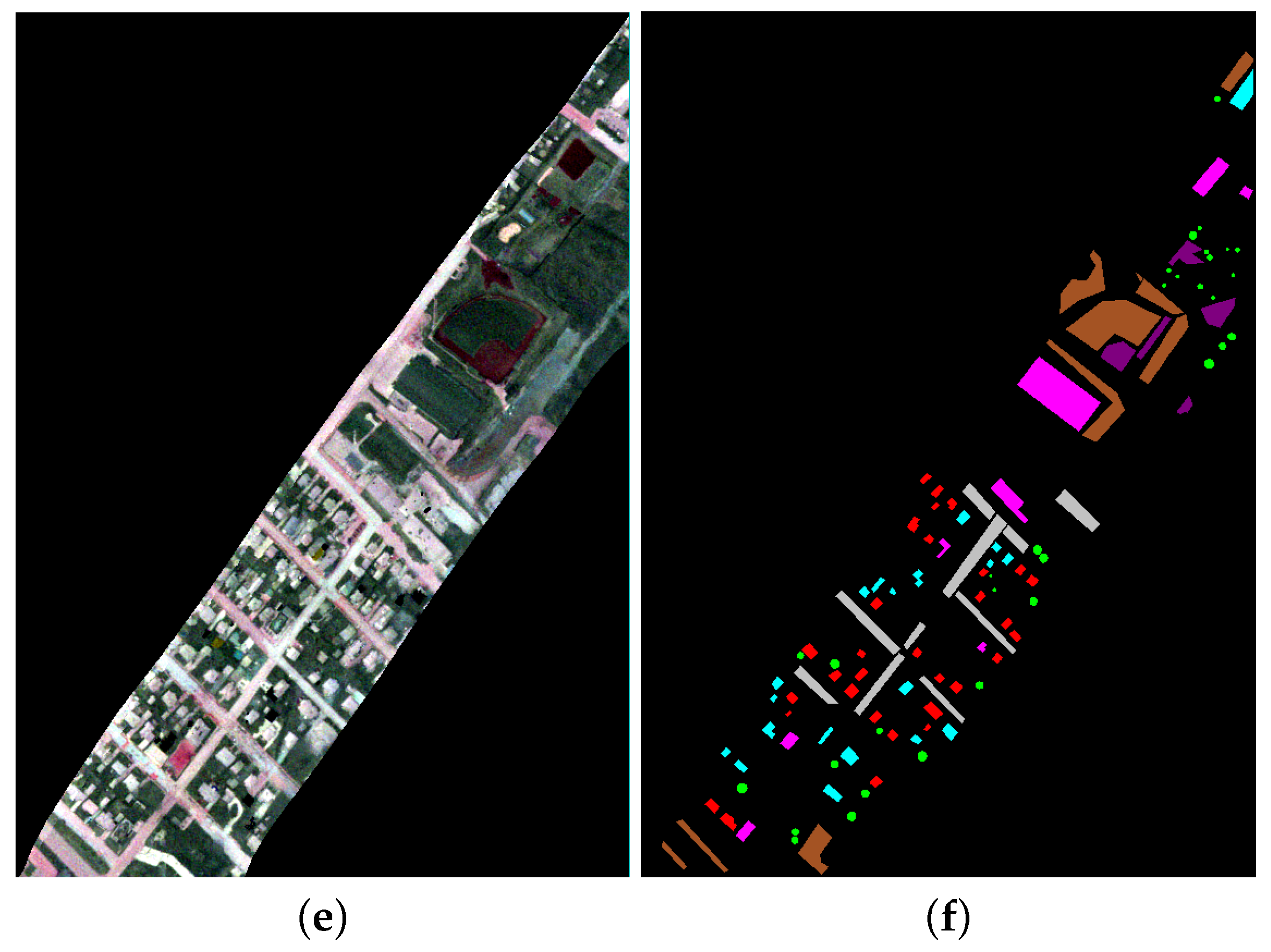
- GRSS_DFC_2014: This is a challenging HSI data set covering an urban area near Thetford Mines in Québec, Canada, and it is used in the 2014 IEEE GRSS Data Fusion Contest. It was acquired by an airborne long-wave infrared hyperspectral imager with 84 channels ranging between 7.8 to 11.5 μm wavelengths. The size of this data set is pixels, and the spatial resolution is about 1 m. In total, 22,532 labeled pixels and a ground truth with seven land cover classes are provided. Some research has indicated that this data set is more challenging for HSI classification [61]. A false color composite image (R-G-B=band 30-45-66) and the corresponding ground truth are shown in Figure 3e,f.
3.3. Classification Results
Classification results by all the compared methods are shown in Figure 4, Figure 5 and Figure 6 and Table 1, Table 2 and Table 3. Since the is a fusion approach of some spectral and spatial features, we especially chose the methods that use single or combine two features for comparison [32,37,46,47], so as to validate the effectiveness of the proposed fusion strategy.
3.3.1. Results on Indian Pines Data Set
Experiments on this data set appear in nearly all the HSI classification works. Maybe, it is because this data set is a little more difficult for classification than some other popular ones such as Salinas or KSC, especially when training samples number is limited. It can be seen from Table 1 that the seven compared methods present various performance with only 20 training samples per class. slightly outperforms HiFi, and achieves 5–10% advantages over other methods. It is worth noting that, in some classes with a large number of testing samples (such as classes 2, 3 and 11), all of the methods present plunges. This is because such few training samples cannot fully represent the data distribution in these classes. On the other hand, we can see from Figure 4 that the spatial consistency is roughly preserved by every one of the methods. Since all of these methods have utilized joint spatial-spectral features, Figure 4 demonstrates that spatial information is really beneficial to HSI classification.
3.3.2. Results on KSC Data Set
It is observed in Figure 5 and Table 2 that results in this data set are much better. Although only 20 samples per class are used for training, presents above 99% accuracies, which achieves about 0.4% advantage. Additionally, we find that reports more than 96% accuracy in each class. Among all of the 13 classes, performs better in nine of them. However, we must recognize that, since most methods have achieved better than 97% OA in this data set, it is not safe to conclude which one is the best. Therefore, experiments on more challenging data sets are of vital importance.
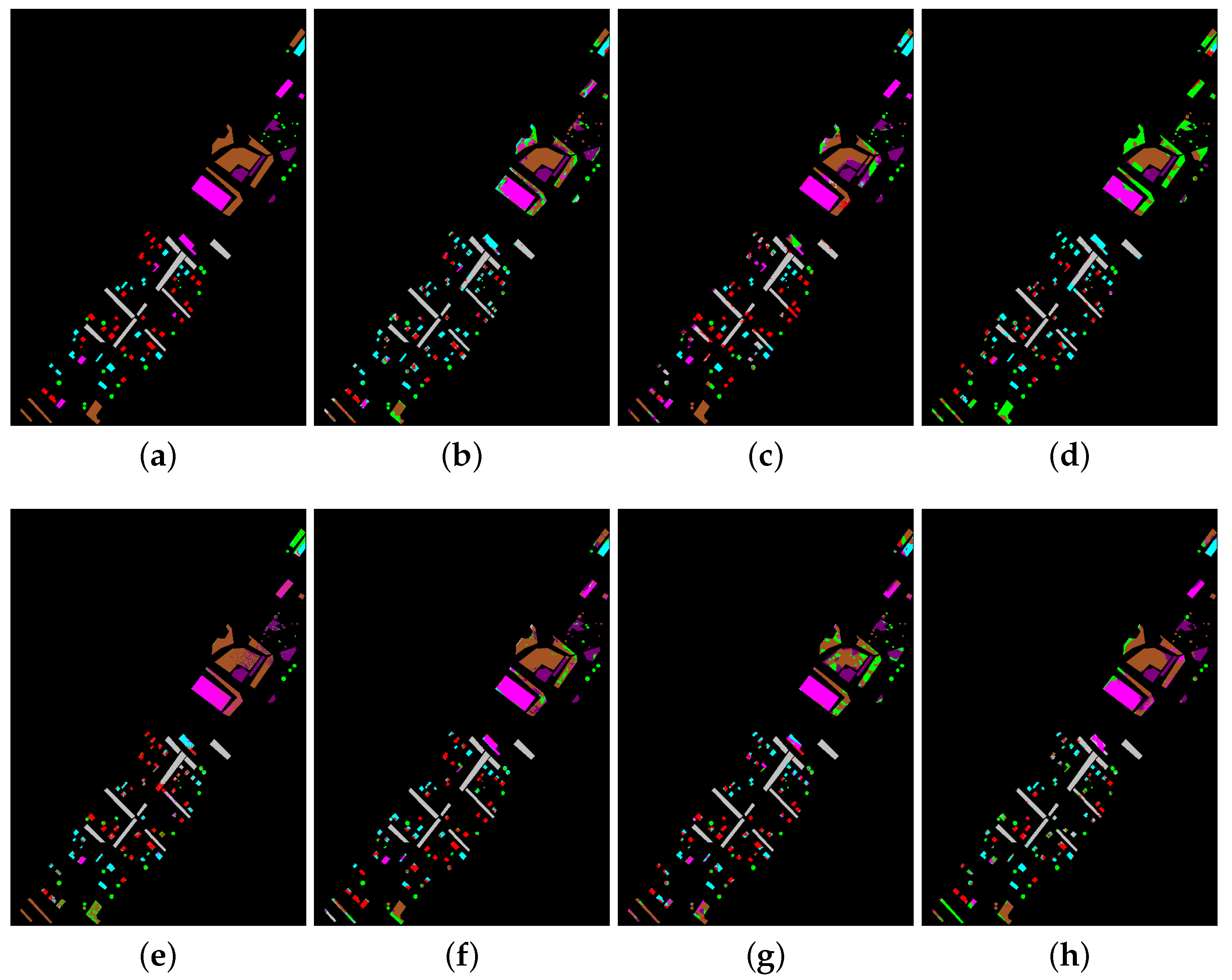
3.3.3. Results on GRSS_DFC_2014 Data Set
Apparently, this data set is more difficult for classification. Although there are still 20 samples per class used for training, accuracies by all the methods present an obvious decline, as shown in Figure 6 and Table 3. The reason may be that the imaging quality in long-wave infrared channels is relatively lower. However, still outperforms other methods by about 2%. Comparison with LGE is especially more meaningful because could be regarded as an improvement of LGE, where we extract the hierarchical features rather than a simple fusion. From Table 1, Table 2 and Table 3, we can find that is slightly better than LGE in all of the three data sets. These results may indicate that the hierarchical strategy in is effective.
3.4. Analysis and Discussion
Figure 7 shows the box plots of OAs by different methods. The box plot is a simple summary for the data distribution. In this paper, we have conducted all the methods 50 times, and the results in each running are displayed by box plots. In a box plot, the red line in the box denotes the median. The top and bottom of a box are the 75th and 25th percentiles, respectively. Data outside the box are mild and extreme outliers. Because LGE, HiFi and present the closest accuracies in the three data sets, we only show the box plots by these methods in Figure 7, and take OA for example. We can see that the boxes of are higher than the others in all the three data sets, and the advantage is more apparent in GRSS_DFC_2014. Moreover, we use a paired t-test to further validate that the improvements by are statistically significant, which is defined as follows:
where and are the OA of and a compared method, and are the corresponding standard deviations, and are the repetition running times, which is set as 50 here, and is the th best quantile of the Student’s law. Results indicate that the improvements by is statistically significant in all of the three data sets (at level 90%).
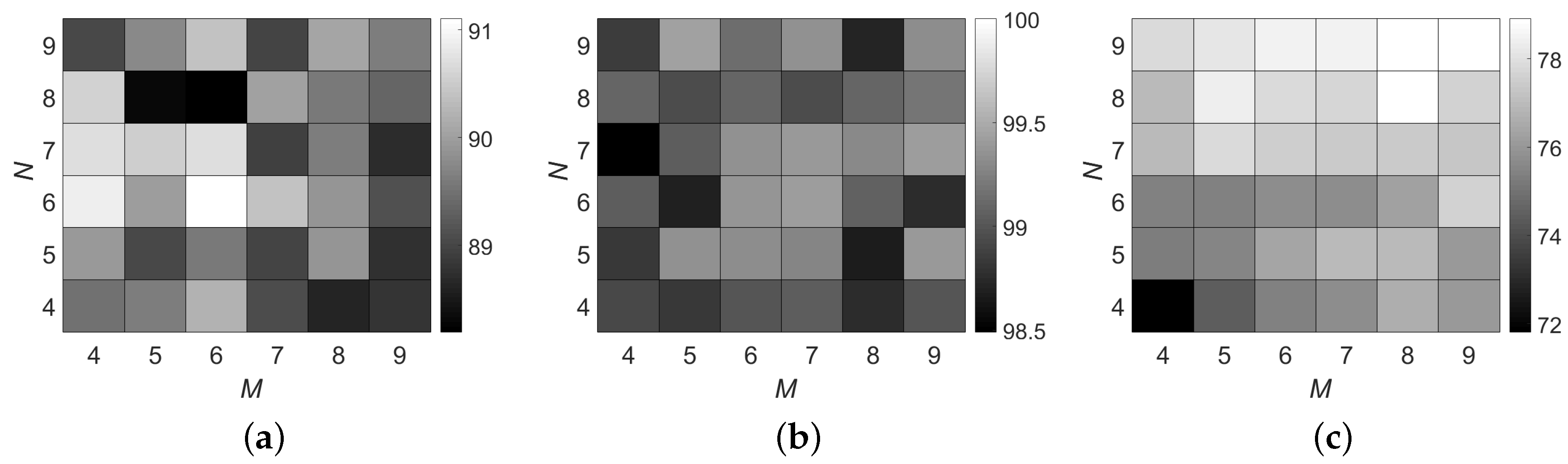
It is worth noting that it is not necessary to tune the parameters in each single feature such as Gabor and RGF. needs to ensemble many groups of features, and setting different parameters is a natural step to generate various sub-features. Therefore, the most important parameters in are the number of sub-feature sets M and the number of features N in each subset. In Figure 8, we provide an analysis for M and N. The results are interesting. We find that, although M and N have drastic changes, the OAs vary little in Indian Pines and KSC data sets. However, in Figure 8c, results demonstrate that more features will contribute to better accuracy. The reason may be that, in the former two data sets, the multiple features have already included some redundancy information. In other words, it is not necessary to extract too many features in Indian Pines and KSC data sets. However, it is not suitable for GRSS_DFC_2014 data set, where further increasing the multiple features would continue improving the classification accuracies. Because GRSS_DFC_2014 is long wave infrared data set, its quality is much lower than that of the other two. It is not appropriate to infer that GRSS_DFC_2014 also has information redundancy. In this case, integrating more features may further enhance the ability of feature representation in GRSS_DFC_2014. Results in Table 3 could also support this opinion. Overall, the most important point we try to emphasize in Figure 8 is that information redundancy does not exist in all of the HSI data. For some popular data sets such as Indian Pines and KSC, maybe information redundancy really exists. However, not all the HSI data includes redundancy information. It is not safe to conclude that dimension reduction could bring competitive or even better classification accuracies. In addition, this is just why we try to extract hierarchical features.
Since the deep features extracted by are usually of high dimension, some popular classifiers such as SVM are time-consuming. In Table 4, we compare the training and testing time by ELM and SVM. To be fair and avoid parameter tuning, linear kernel is adopted by both of them. Another advantage of using linear kernel is that it could reduce the computational complexity. Furthermore, the OAs by ELM and SVM are also reported. Note that the running time in Table 4 is only composed of the classifiers’ training and testing process, not including the feature extraction process. We can see from Table 4 that ELM presents slightly better performance than SVM with lower computational consumption. Because the selection of classifier is not the emphasis in , we choose ELM according to the results in Table 4.
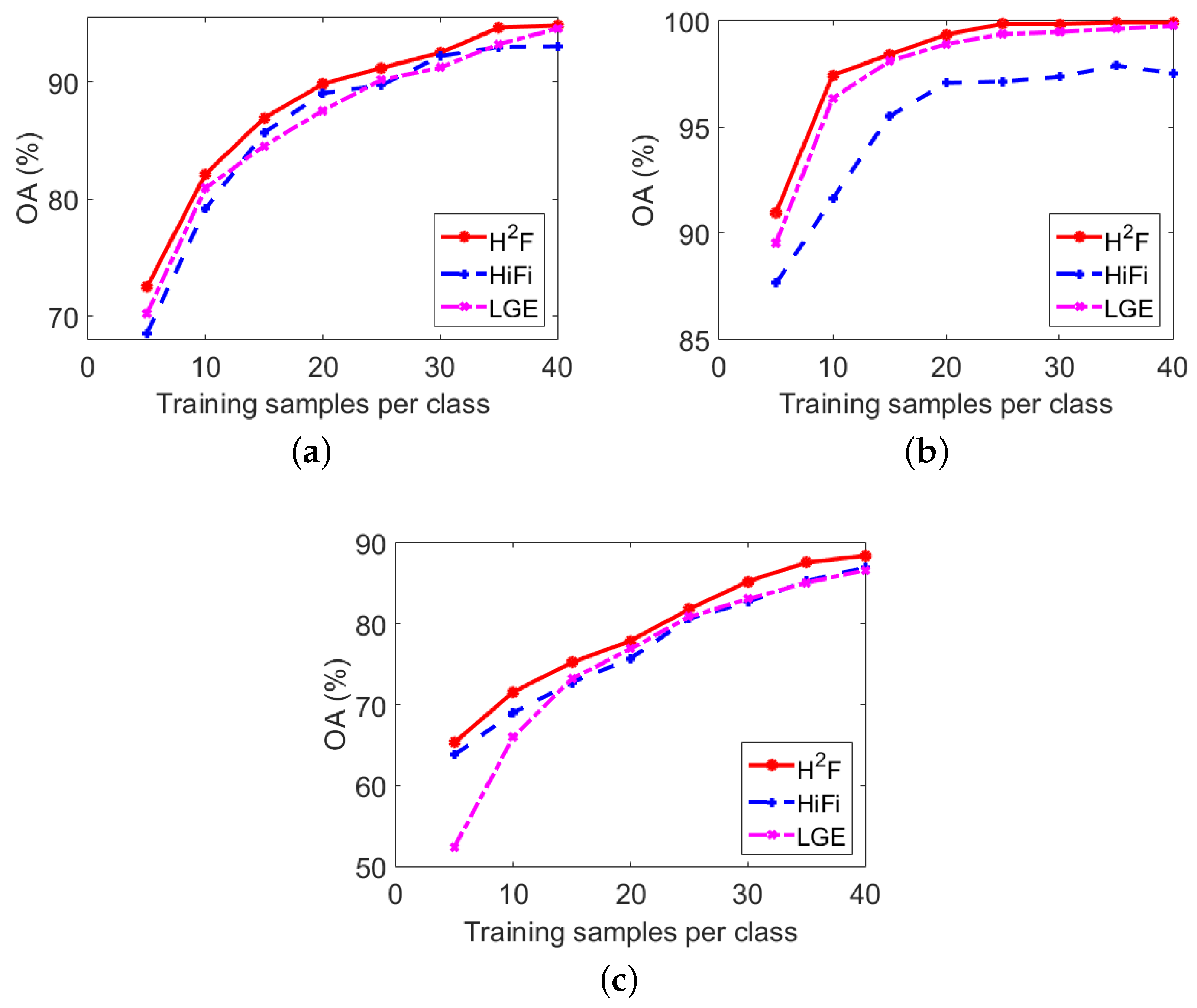
Finally, we give an evaluation for the influence of training samples number in Figure 9. Classes with totally 20 around samples are ignored because they have little influence on OA. Similar to Figure 7, HiFi and LGE are used for comparison. As is expected, the accuracy improves with the increase of training samples number. outperforms the others in most cases. In particular, we note that the gaps are more apparent when training samples are limited. This results may indicate that could provide more representative feature expression for the original HSI data.
4. Conclusions
In this paper, we proposed a hierarchical feature extraction method for HSI classification. The proposed method is inspired by the promising performance of multiple features fusion. We hold the opinion that further utilization for the multiple features will contribute to the classification accuracy, and this idea is similar to that of deep learning methods. Therefore, instead of data dimension reduction or direct ensembling, in , we propose a hierarchical feature extraction strategy based on hashing, which attempts to explore the deep distinctive information among the original HSI data. Spectral as well as local and global spatial features are firstly extracted, and these low-level features are further represented in a very sparse manner.
We compare with some ensemble based or deep learning based methods in the experimental part. Although the advantages are not apparent, a paired t-test has confirmed that our improvements are statistically significant. In particular, the idea of extracting hierarchical information from basic features may work as an inspiration for the further research.
In our future works, we will focus on improving the computational efficiency of the hierarchical feature extraction process. Meanwhile, the relationships among different features should also be investigated.
Acknowledgments
The authors would like to thank Telops Inc. (Québec, Canada) for acquiring and providing the data used in this study, the IEEE GRSS Image Analysis and Data Fusion Technical Committee and Michal Shimoni (Signal and Image Centre, Royal Military Academy, Belgium) for organizing the 2014 Data Fusion Contest, the Centre de Recherche Public Gabriel Lippmann (CRPGL, Luxembourg) and Martin Schlerf (CRPGL) for their contribution of the Hyper-Cam LWIR sensor, and Michaela De Martino (University of Genoa, Italy) for her contribution to data preparation. The work was supported by the National Natural Science Foundation of China under the Grant 61671037, and the Beijing Natural Science Foundation under the Grant 4152031, and the Excellence Foundation of BUAA for PhD Students under Grant 2017057.
Author Contributions
Bin Pan and Zhenwei Shi designed the algorithm; Xia Xu designed and performed the experiments; Yi Yang contributed to the English expression of this paper; Bin Pan wrote the paper.
Conflicts of Interest
The authors declare no conflict of interest.
References
- Fu, Y.; Zhao, C.; Wang, J.; Jia, X.; Yang, G.; Song, X.; Feng, H. An Improved Combination of Spectral and Spatial Features for Vegetation Classification in Hyperspectral Images. Remote Sens. 2017, 9, 261. [Google Scholar] [CrossRef]
- Pan, B.; Shi, Z.; An, Z.; Jiang, Z.; Ma, Y. A Novel Spectral-Unmixing-Based Green Algae Area Estimation Method for GOCI Data. IEEE J. Sel. Top. Appl. Earth Obs. Remote Sens. 2017, 10, 437–449. [Google Scholar] [CrossRef]
- Kang, X.; Zhang, X.; Li, S.; Li, K.; Li, J.; Benediktsson, J.A. Hyperspectral Anomaly Detection With Attribute and Edge-Preserving Filters. IEEE Trans. Geosci. Remote Sens. 2017, 55, 5600–5611. [Google Scholar] [CrossRef]
- Xu, X.; Shi, Z. Multi-objective based spectral unmixing for hyperspectral images. ISPRS J. Photogramm. Remote Sens. 2017, 124, 54–69. [Google Scholar] [CrossRef]
- Zhong, P.; Zhang, P.; Wang, R. Dynamic Learning of SMLR for Feature Selection and Classification of Hyperspectral Data. IEEE Geosci. Remote Sens. Lett. 2008, 5, 280–284. [Google Scholar] [CrossRef]
- Gomez-Chova, L.; Camps-Valls, G.; Munoz-Mari, J.; Calpe, J. Semisupervised Image Classification with Laplacian Support Vector Machines. IEEE Geosci. Remote Sens. Lett. 2008, 5, 336–340. [Google Scholar] [CrossRef]
- Pal, M.; Foody, G.M. Feature Selection for Classification of Hyperspectral Data by SVM. IEEE Trans. Geosci. Remote Sens. 2010, 48, 2297–2307. [Google Scholar] [CrossRef]
- Mountrakis, G.; Im, J.; Ogole, C. Support vector machines in remote sensing: A review. ISPRS J. Photogramm. Remote Sens. 2011, 66, 247–259. [Google Scholar] [CrossRef]
- Castrodad, A.; Xing, Z.; Greer, J.B.; Bosch, E.; Carin, L.; Sapiro, G. Learning discriminative sparse representations for modeling, source separation, and mapping of hyperspectral imagery. IEEE Trans. Geosci. Remote Sens. 2011, 49, 4263–4281. [Google Scholar] [CrossRef]
- Li, J.; Bioucas-Dias, J.M.; Plaza, A. Spectral-spatial hyperspectral image segmentation using subspace multinomial logistic regression and Markov random fields. IEEE Trans. Geosci. Remote Sens. 2012, 50, 809–823. [Google Scholar] [CrossRef]
- Li, W.; Prasad, S.; Fowler, J.E. Hyperspectral image classification using Gaussian mixture models and Markov random fields. IEEE Geosci. Remote Sens. Lett. 2014, 11, 153–157. [Google Scholar] [CrossRef]
- Tarabalka, Y.; Fauvel, M.; Chanussot, J.; Benediktsson, J.A. SVM-and MRF-based method for accurate classification of hyperspectral images. IEEE Geosci. Remote Sens. Lett. 2010, 7, 736–740. [Google Scholar] [CrossRef]
- Benediktsson, J.A.; Palmason, J.A.; Sveinsson, J.R. Classification of hyperspectral data from urban areas based on extended morphological profiles. IEEE Trans. Geosci. Remote Sens. 2005, 43, 480–491. [Google Scholar] [CrossRef]
- Dalla Mura, M.; Atli Benediktsson, J.; Waske, B.; Bruzzone, L. Extended profiles with morphological attribute filters for the analysis of hyperspectral data. Int. J. Remote Sens. 2010, 31, 5975–5991. [Google Scholar] [CrossRef]
- Zhong, Z.; Fan, B.; Ding, K.; Li, H.; Xiang, S.; Pan, C. Efficient Multiple Feature Fusion With Hashing for Hyperspectral Imagery Classification: A Comparative Study. IEEE Trans. Geosci. Remote Sens. 2016, 54, 4461–4478. [Google Scholar] [CrossRef]
- Li, J.; Marpu, P.R.; Plaza, A.; Bioucas-Dias, J.M.; Benediktsson, J.A. Generalized composite kernel framework for hyperspectral image classification. IEEE Trans. Geosci. Remote Sens. 2013, 51, 4816–4829. [Google Scholar] [CrossRef]
- Gu, Y.; Liu, T.; Jia, X.; Benediktsson, J.A.; Chanussot, J. Nonlinear multiple kernel learning with multiple-structure-element extended morphological profiles for hyperspectral image classification. IEEE Trans. Geosci. Remote Sens. 2016, 54, 3235–3247. [Google Scholar] [CrossRef]
- Liu, T.; Gu, Y.; Jia, X.; Benediktsson, J.A.; Chanussot, J. Class-Specific Sparse Multiple Kernel Learning for Spectral–Spatial Hyperspectral Image Classification. IEEE Trans. Geosci. Remote Sens. 2016, 54, 7351–7365. [Google Scholar] [CrossRef]
- Wang, Q.; Gu, Y.; Tuia, D. Discriminative multiple kernel learning for hyperspectral image classification. IEEE Trans. Geosci. Remote Sens. 2016, 54, 3912–3927. [Google Scholar] [CrossRef]
- Zhang, Q.; Tian, Y.; Yang, Y.; Pan, C. Automatic Spatial–Spectral Feature Selection for Hyperspectral Image via Discriminative Sparse Multimodal Learning. IEEE Trans. Geosci. Remote Sens. 2015, 53, 261–279. [Google Scholar] [CrossRef]
- Zhang, L.; Zhang, Q.; Du, B.; Huang, X.; Tang, Y.Y.; Tao, D. Simultaneous Spectral-Spatial Feature Selection and Extraction for Hyperspectral Images. IEEE Trans. Cybern. 2017, PP, 1–13. [Google Scholar] [CrossRef] [PubMed]
- Zhang, L.; Zhang, L.; Tao, D.; Huang, X. On Combining Multiple Features for Hyperspectral Remote Sensing Image Classification. IEEE Trans. Geosci. Remote Sens. 2012, 50, 879–893. [Google Scholar] [CrossRef]
- Zhang, L.; Zhang, L.; Tao, D.; Huang, X. A modified stochastic neighbor embedding for multi-feature dimension reduction of remote sensing images. ISPRS J. Photogramm. Remote Sens. 2013, 83, 30–39. [Google Scholar] [CrossRef]
- Wang, M.; Yu, J.; Niu, L.; Sun, W. Feature Extraction for Hyperspectral Images Using Low-Rank Representation With Neighborhood Preserving Regularization. IEEE Geosci. Remote Sens. Lett. 2017, 14, 836–840. [Google Scholar]
- Zhou, Z.H. Ensemble Methods: Foundations and Algorithms; CRC Press: Boca Raton, FL, USA, 2012. [Google Scholar]
- Pal, M. Ensemble of support vector machines for land cover classification. Int. J. Remote Sens. 2008, 29, 3043–3049. [Google Scholar] [CrossRef]
- Huang, X.; Zhang, L. An SVM ensemble approach combining spectral, structural, and semantic features for the classification of high-resolution remotely sensed imagery. IEEE Trans. Geosci. Remote Sens. 2013, 51, 257–272. [Google Scholar] [CrossRef]
- Liu, Z.; Tang, B.; He, X.; Qiu, Q.; Liu, F. Class-Specific Random Forest With Cross-Correlation Constraints for Spectral–Spatial Hyperspectral Image Classification. IEEE Geosci. Remote Sens. Lett. 2017, 14, 257–261. [Google Scholar] [CrossRef]
- Xia, J.; Bombrun, L.; Adalı, T.; Berthoumieu, Y.; Germain, C. Spectral–spatial classification of hyperspectral images using ica and edge-preserving filter via an ensemble strategy. IEEE Trans. Geosci. Remote Sens. 2016, 54, 4971–4982. [Google Scholar] [CrossRef]
- Xia, J.; Falco, N.; Benediktsson, J.A.; Du, P.; Chanussot, J. Hyperspectral Image Classification With Rotation Random Forest Via KPCA. IEEE J. Sel. Top. Appl. Earth Obs. Remote Sens. 2017, 10, 1601–1609. [Google Scholar] [CrossRef]
- Chen, J.; Wang, C.; Wang, R. Using stacked generalization to combine SVMs in magnitude and shape feature spaces for classification of hyperspectral data. IEEE Trans. Geosci. Remote Sens. 2009, 47, 2193–2205. [Google Scholar] [CrossRef]
- Pan, B.; Shi, Z.; Xu, X. Hierarchical Guidance Filtering-Based Ensemble Classification for Hyperspectral Images. IEEE Trans. Geosci. Remote Sens. 2017, 55, 4177–4189. [Google Scholar] [CrossRef]
- Debes, C.; Merentitis, A.; Heremans, R.; Hahn, J.; Frangiadakis, N.; Kasteren, T.V.; Liao, W.; Bellens, R.; Pižurica, A.; Gautama, S. Hyperspectral and LiDAR Data Fusion: Outcome of the 2013 GRSS Data Fusion Contest. IEEE J. Sel. Top. Appl. Earth Obs. Remote Sens. 2014, 7, 2405–2418. [Google Scholar] [CrossRef]
- Liao, W.; Pižurica, A.; Bellens, R.; Gautama, S.; Philips, W. Generalized Graph-Based Fusion of Hyperspectral and LiDAR Data Using Morphological Features. IEEE Geosci. Remote Sens. Lett. 2015, 12, 552–556. [Google Scholar] [CrossRef]
- Chen, Y.; Lin, Z.; Zhao, X.; Wang, G.; Gu, Y. Deep learning-based classification of hyperspectral data. IEEE J. Sel. Top. Appl. Earth Obs. Remote Sens. 2014, 7, 2094–2107. [Google Scholar] [CrossRef]
- Pan, B.; Shi, Z.; Zhang, N.; Xie, S. Hyperspectral Image Classification Based on Nonlinear Spectral–Spatial Network. IEEE Geosci. Remote Sens. Lett. 2016, 13, 1782–1786. [Google Scholar] [CrossRef]
- Pan, B.; Shi, Z.; Xu, X. R-VCANet: A new deep-learning-based hyperspectral image classification method. IEEE J. Sel. Top. Appl. Earth Obs. Remote Sens. 2017, 10, 1975–1986. [Google Scholar] [CrossRef]
- Wu, H.; Prasad, S. Convolutional Recurrent Neural Networks for Hyperspectral Data Classification. Remote Sens. 2017, 9, 298. [Google Scholar] [CrossRef]
- Ding, C.; Li, Y.; Xia, Y.; Wei, W.; Zhang, L.; Zhang, Y. Convolutional Neural Networks Based Hyperspectral Image Classification Method with Adaptive Kernels. Remote Sens. 2017, 9. [Google Scholar] [CrossRef]
- Li, W.; Wu, G.; Zhang, F.; Du, Q. Hyperspectral image classification using deep pixel-pair features. IEEE Trans. Geosci. Remote Sens. 2017, 55, 844–853. [Google Scholar] [CrossRef]
- He, K.; Zhang, X.; Ren, S.; Sun, J. Delving deep into rectifiers: Surpassing human-level performance on ImageNet classification. In Proceedings of the IEEE International Conference on Computer Vision, Santiago, Chile, 7–13 December 2015; pp. 1026–1034. [Google Scholar]
- Zhong, P.; Gong, Z.; Li, S.; Schonlieb, C.B. Learning to Diversify Deep Belief Networks for Hyperspectral Image Classification. IEEE Trans. Geosci. Remote Sens. 2017, 55, 3516–3530. [Google Scholar] [CrossRef]
- Liang, H.; Li, Q. Hyperspectral Imagery Classification Using Sparse Representations of Convolutional Neural Network Features. Remote Sens. 2016, 8, 99. [Google Scholar] [CrossRef]
- Li, Y.; Zhang, H.; Shen, Q. Spectral–Spatial Classification of Hyperspectral Imagery with 3D Convolutional Neural Network. Remote Sens. 2017, 9, 67. [Google Scholar] [CrossRef]
- Zhang, Q.; Shen, X.; Xu, L.; Jia, J. Rolling Guidance Filter. In Proceedings of the European Conference on Computer Vision, Zurich, Switzerland, 6–12 September 2014; pp. 815–830. [Google Scholar]
- Li, W.; Chen, C.; Su, H.; Du, Q. Local Binary Patterns and Extreme Learning Machine for Hyperspectral Imagery Classification. IEEE Trans. Geosci. Remote Sens. 2015, 53, 3681–3693. [Google Scholar] [CrossRef]
- Li, W.; Du, Q. Gabor-Filtering-Based Nearest Regularized Subspace for Hyperspectral Image Classification. IEEE J. Sel. Top. Appl. Earth Obs. Remote Sens. 2014, 7, 1012–1022. [Google Scholar] [CrossRef]
- Xu, X.; Shi, Z.; Pan, B. A New Unsupervised Hyperspectral Band Selection Method Based on Multiobjective Optimization. IEEE Geosci. Remote Sens. Lett. 2017, PP, 1–5. [Google Scholar] [CrossRef]
- Cavallaro, G.; Falco, N.; Mura, M.D.; Benediktsson, J.A. Automatic Attribute Profiles. IEEE Trans. Image Process. 2017, 26, 1859–1872. [Google Scholar]
- Kang, X.; Xiang, X.; Li, S.; Benediktsson, J.A. PCA-Based Edge-Preserving Features for Hyperspectral Image Classification. IEEE Trans. Geosci. Remote Sens. 2017, PP, 1–12. [Google Scholar] [CrossRef]
- Huang, G.B.; Zhu, Q.Y.; Siew, C.K. Extreme learning machine: Theory and applications. Neurocomputing 2006, 70, 489–501. [Google Scholar] [CrossRef]
- Samat, A.; Du, P.; Liu, S.; Li, J.; Cheng, L. E2LMs : Ensemble Extreme Learning Machines for Hyperspectral Image Classification. IEEE J. Sel. Top. Appl. Earth Obs. Remote Sens. 2014, 7, 1060–1069. [Google Scholar] [CrossRef]
- Su, H.; Cai, Y.; Du, Q. Firefly-Algorithm-Inspired Framework With Band Selection and Extreme Learning Machine for Hyperspectral Image Classification. IEEE J. Sel. Top. Appl. Earth Obs. Remote Sens. 2017, 10, 309–320. [Google Scholar]
- He, K.; Sun, J.; Tang, X. Guided image filtering. IEEE Trans. Pattern Anal. Mach. Intell. 2013, 35, 1397–1409. [Google Scholar] [CrossRef] [PubMed]
- Friedman, J.; Hastie, T.; Tibshirani, R. The Elements of Statistical Learning; Springer Series in Statistics; Springer: Berlin, Germany, 2001; Volume 1. [Google Scholar]
- Bau, T.C.; Sarkar, S.; Healey, G. Hyperspectral region classification using a three-dimensional Gabor filterbank. IEEE Trans. Geosci. Remote Sens. 2010, 48, 3457–3464. [Google Scholar] [CrossRef]
- Shen, L.; Jia, S. Three-dimensional Gabor wavelets for pixel-based hyperspectral imagery classification. IEEE Trans. Geosci. Remote Sens. 2011, 49, 5039–5046. [Google Scholar] [CrossRef]
- Kang, X.; Li, S.; Benediktsson, J.A. Spectral–Spatial Hyperspectral Image Classification with Edge-Preserving Filtering. IEEE Trans. Geosci. Remote Sens. 2014, 52, 2666–2677. [Google Scholar] [CrossRef]
- Kang, X.; Li, S.; Fang, L.; Benediktsson, J.A. Intrinsic Image Decomposition for Feature Extraction of Hyperspectral Images. IEEE Trans. Geosci. Remote Sens. 2015, 53, 2241–2253. [Google Scholar] [CrossRef]
- 2014 IEEE GRSS Data Fusion Contest. Available online: http://www.grss-ieee.org/community/technical-committees/data-fusion/ (accessed on 25 October 2017).
- Liao, W.; Huang, X.; Coillie, F.V.; Gautama, S.; Pižurica, A.; Philips, W.; Liu, H.; Zhu, T.; Shimoni, M.; Moser, G. Processing of Multiresolution Thermal Hyperspectral and Digital Color Data: Outcome of the 2014 IEEE GRSS Data Fusion Contest. IEEE J. Sel. Top. Appl. Earth Obs. Remote Sens. 2015, 8, 2984–2996. [Google Scholar] [CrossRef]
- Sun, B.; Kang, X.; Li, S.; Benediktsson, J.A. Random-Walker-Based Collaborative Learning for Hyperspectral Image Classification. IEEE Trans. Geosci. Remote Sens. 2017, 55, 212–222. [Google Scholar] [CrossRef]
Figure 1.
The flowchart of the based method.

Figure 2.
An illustration for the hashing based hierarchical feature representation. This figure only presents the process in one pixel and a single sub-feature set.
Figure 2.
An illustration for the hashing based hierarchical feature representation. This figure only presents the process in one pixel and a single sub-feature set.
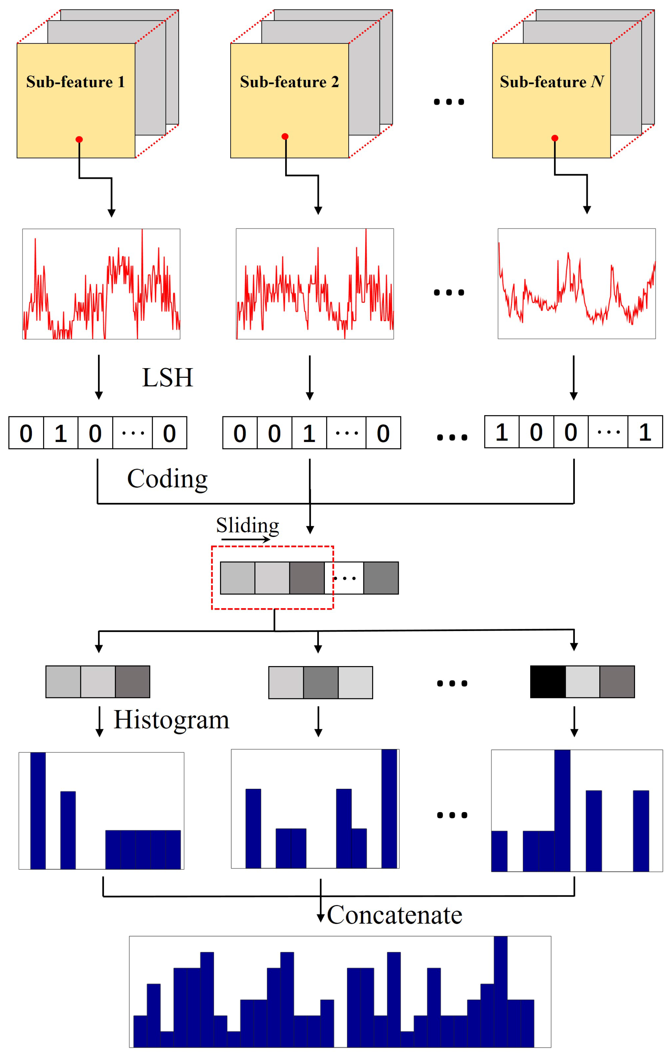
Figure 3.
False color composite images of (a) Indian Pines; (c) KSC and (e) GRSS_DFC_2014 data sets and the ground truths (b,d,f). Each color corresponds to a certain class.
Figure 3.
False color composite images of (a) Indian Pines; (c) KSC and (e) GRSS_DFC_2014 data sets and the ground truths (b,d,f). Each color corresponds to a certain class.
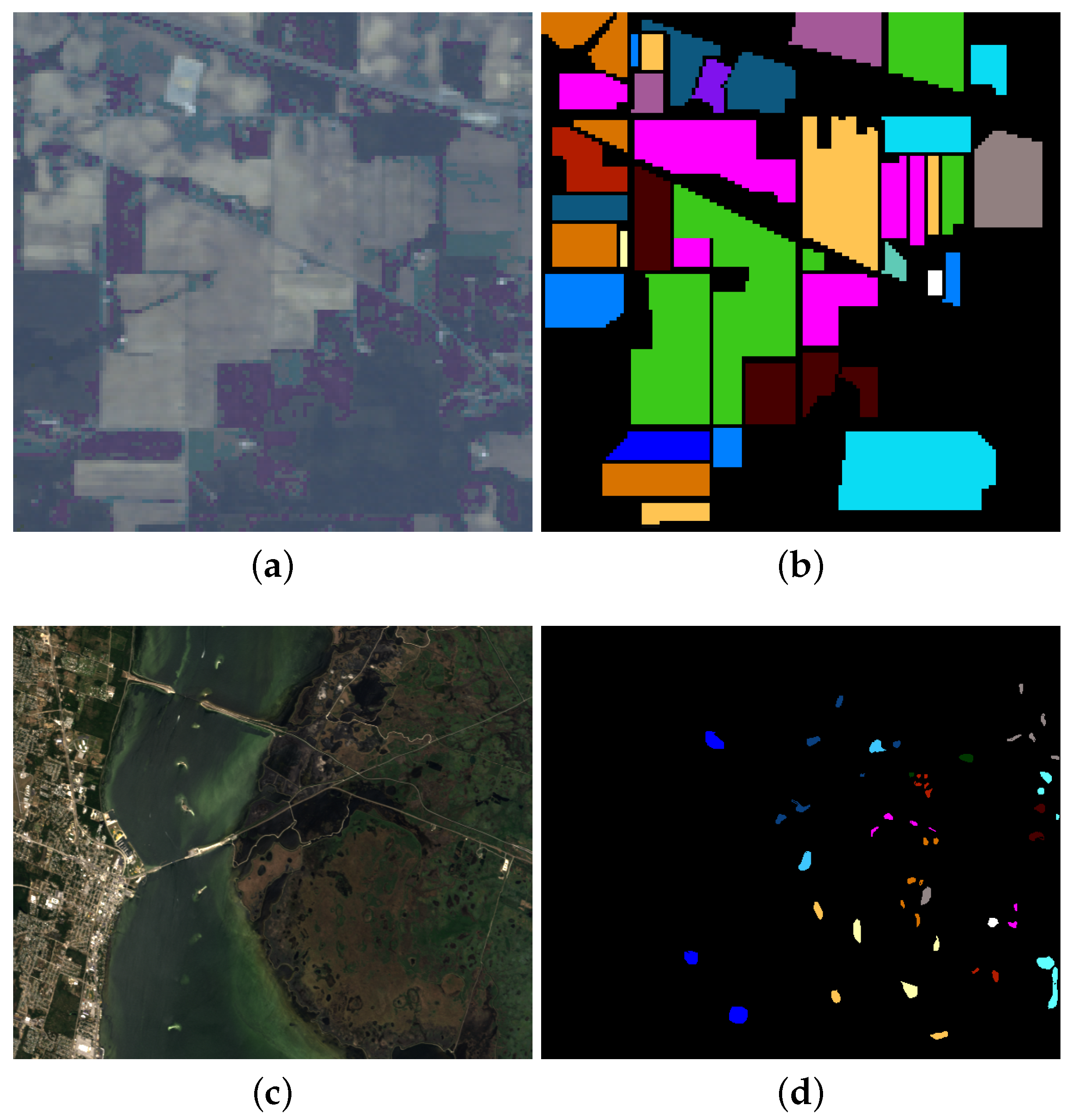

Figure 4.
Classification maps by compared methods for Indian Pines data set. (a) The ground truth (b) GE (c) LGE (d) EPF (e) IIDF (f) RVCANet (g) HiFi (h) .
Figure 4.
Classification maps by compared methods for Indian Pines data set. (a) The ground truth (b) GE (c) LGE (d) EPF (e) IIDF (f) RVCANet (g) HiFi (h) .

Figure 5.
Classification maps by compared methods for KSC data set. (a) the ground truth; (b) GE; (c) LGE; (d) EPF; (e) IIDF; (f) RVCANet; (g) HiFi; (h) .
Figure 5.
Classification maps by compared methods for KSC data set. (a) the ground truth; (b) GE; (c) LGE; (d) EPF; (e) IIDF; (f) RVCANet; (g) HiFi; (h) .
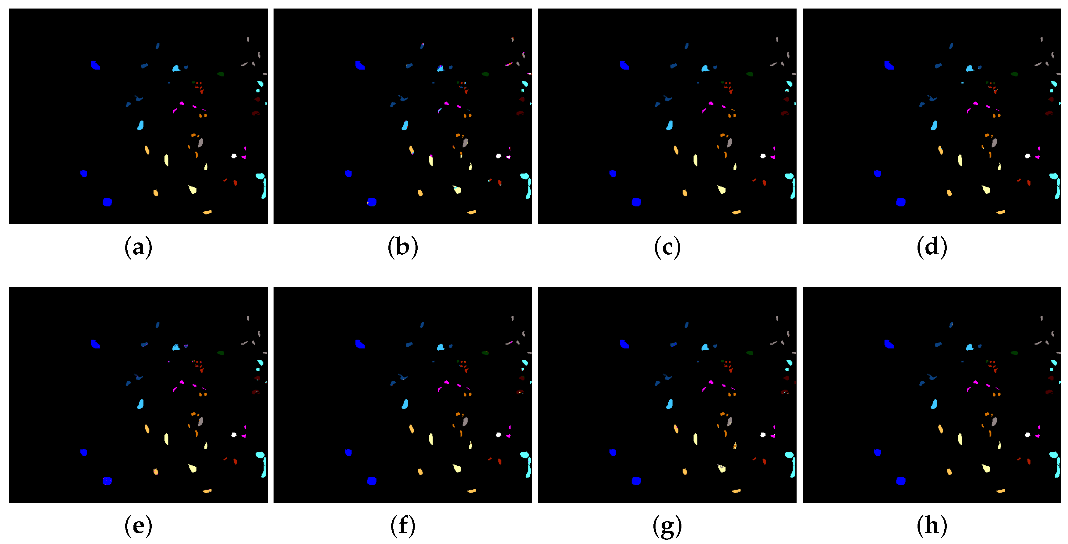
Figure 6.
Classification maps by compared methods for GRSS_DFC_2014 data set. (a) the ground truth; (b) GE; (c) LGE; (d) EPF; (e) IIDF; (f) RVCANet; (g) HiFi; (h) .
Figure 6.
Classification maps by compared methods for GRSS_DFC_2014 data set. (a) the ground truth; (b) GE; (c) LGE; (d) EPF; (e) IIDF; (f) RVCANet; (g) HiFi; (h) .

Figure 7.
Box plots of different methods on (a) Indian Pines; (b) KSC and (c) GRSS_DFC_2014 data sets.
Figure 7.
Box plots of different methods on (a) Indian Pines; (b) KSC and (c) GRSS_DFC_2014 data sets.
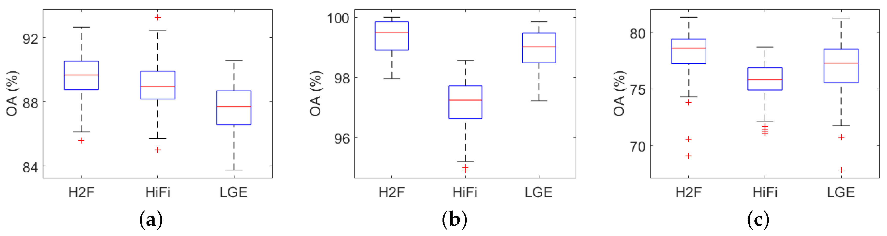
Figure 8.
The influence of parameters on OA (%) in . Results on (a) Indian Pines; (b) KSC and (c) GRSS_DFC_2014 data sets. M is the number of sub-feature sets, and N is the number of features in each subsets.
Figure 8.
The influence of parameters on OA (%) in . Results on (a) Indian Pines; (b) KSC and (c) GRSS_DFC_2014 data sets. M is the number of sub-feature sets, and N is the number of features in each subsets.

Figure 9.
Influence of training samples number on (a) Indian Pines; (b) KSC and (c) GRSS_DFC_2014 data sets.
Figure 9.
Influence of training samples number on (a) Indian Pines; (b) KSC and (c) GRSS_DFC_2014 data sets.

Table 1.
Classification accuracies of different methods on Indian Pines data set (%).
| Class | Samples | Methods | ||||||
|---|---|---|---|---|---|---|---|---|
| Train/Test | GE | LGE | EPF | IIDF | RCANet | HiFi | ||
| C1 | 20/26 | 99.42 ± 0.55 | 99.92 ± 0.54 | 98.84 ± 1.78 | 87.22 ± 14.9 | 99.00 ± 1.70 | 99.46 ± 1.35 | 100.0 ± 0.00 |
| C2 | 20/1408 | 70.45 ± 7.42 | 80.89 ± 5.30 | 56.53 ± 11.1 | 80.45 ± 6.04 | 63.94 ± 6.85 | 81.91 ± 5.58 | 81.88 ± 5.29 |
| C3 | 20/810 | 74.25 ± 7.71 | 85.61 ± 7.03 | 67.27 ± 10.5 | 75.89 ± 6.86 | 79.91 ± 7.05 | 91.49 ± 4.52 | 87.00 ± 5.86 |
| C4 | 20/217 | 95.10 ± 4.59 | 99.40 ± 1.14 | 96.56 ± 4.60 | 66.03 ± 10.8 | 98.59 ± 2.22 | 96.78 ± 3.84 | 99.21 ± 1.30 |
| C5 | 20/463 | 87.51 ± 5.18 | 92.13 ± 5.39 | 91.09 ± 4.56 | 93.49 ± 4.30 | 93.60 ± 3.02 | 90.06 ± 3.88 | 90.53 ± 4.21 |
| C6 | 20/710 | 92.35 ± 4.19 | 94.99 ± 3.72 | 96.97 ± 3.93 | 97.67 ± 2.11 | 98.36 ± 1.10 | 97.92 ± 1.80 | 97.21 ± 2.11 |
| C7 | 14/14 | 100.0 ± 0.00 | 100.0 ± 0.00 | 96.85 ± 3.58 | 54.08 ± 20.6 | 100.0 ± 0.00 | 96.75 ± 5.54 | 100.0 ± 0.00 |
| C8 | 20/458 | 98.56 ± 2.30 | 99.83 ± 0.52 | 96.65 ± 5.47 | 99.91 ± 0.14 | 98.76 ± 0.63 | 99.39 ± 0.92 | 99.98 ± 0.10 |
| C9 | 10/10 | 99.59 ± 0.35 | 100.0 ± 0.00 | 99.80 ± 1.41 | 44.83 ± 19.7 | 100.0 ± 0.00 | 100.0 ± 0.00 | 100.0 ± 0.00 |
| C10 | 20/952 | 73.53 ± 8.16 | 86.55 ± 5.72 | 83.09 ± 7.85 | 73.57 ± 8.49 | 87.43 ± 3.79 | 88.16 ± 6.63 | 88.97 ± 4.47 |
| C11 | 20/2435 | 69.93 ± 8.38 | 79.21 ± 5.37 | 69.55 ± 9.23 | 92.37 ± 3.52 | 72.01 ± 6.49 | 79.82 ± 5.86 | 83.97 ± 5.30 |
| C12 | 20/573 | 81.23 ± 7.01 | 85.11 ± 5.95 | 73.26 ± 10.1 | 79.13 ± 6.94 | 90.49 ± 4.08 | 93.31 ± 3.18 | 87.61 ± 5.72 |
| C13 | 20/185 | 98.76 ± 1.28 | 99.58 ± 1.16 | 99.39 ± 0.32 | 99.54 ± 1.53 | 99.49 ± 0.31 | 99.41 ± 0.29 | 99.84 ± 0.31 |
| C14 | 20/1245 | 87.16 ± 5.11 | 96.47 ± 3.63 | 88.51 ± 7.76 | 99.06 ± 1.04 | 94.24 ± 3.49 | 96.96 ± 2.79 | 96.70 ± 3.25 |
| C15 | 20/366 | 90.80 ± 6.09 | 98.21 ± 2.83 | 81.44 ± 10.6 | 84.73 ± 11.1 | 90.65 ± 4.05 | 95.23 ± 2.72 | 98.46 ± 4.23 |
| C16 | 20/73 | 98.65 ± 2.02 | 98.30 ± 2.45 | 96.93 ± 5.68 | 94.62 ± 6.86 | 99.06 ± 1.90 | 99.07 ± 0.65 | 99.75 ± 0.53 |
| OA | 79.38 ± 1.82 | 87.61 ± 1.48 | 77.54 ± 3.10 | 85.89 ± 1.88 | 83.06 ± 2.32 | 89.06 ± 1.70 | 89.55 ± 1.31 | |
| AA | 88.58 ± 1.03 | 93.51 ± 0.69 | 87.04 ± 1.88 | 82.66 ± 2.22 | 91.56 ± 0.89 | 94.11 ± 0.77 | 94.44 ± 0.73 | |
| 76.60 ± 2.03 | 85.99 ± 1.64 | 74.66 ± 3.41 | 84.02 ± 2.11 | 80.87 ± 2.56 | 87.51 ± 1.90 | 88.15 ± 1.49 | ||
Table 2.
Classification accuracies of different methods on the KSC data set (%).
| Class | Samples | Methods | ||||||
|---|---|---|---|---|---|---|---|---|
| Train/Test | GE | LGE | EPF | IIDF | RCANet | HiFi | ||
| C1 | 20/741 | 93.54 ± 2.63 | 98.84 ± 1.87 | 99.43 ± 1.13 | 99.86 ± 0.22 | 97.80 ± 1.65 | 98.60 ± 1.06 | 99.97 ± 0.11 |
| C2 | 20/223 | 68.04 ± 6.48 | 95.69 ± 5.98 | 89.65 ± 6.84 | 94.80 ± 5.55 | 95.74 ± 4.30 | 92.26 ± 5.02 | 97.04 ± 5.21 |
| C3 | 20/236 | 84.24 ± 7.53 | 99.43 ± 1.70 | 97.39 ± 1.93 | 99.42 ± 0.91 | 98.33 ± 1.39 | 96.42 ± 3.31 | 99.88 ± 0.56 |
| C4 | 20/232 | 75.14 ± 6.79 | 98.49 ± 3.04 | 93.84 ± 6.78 | 96.42 ± 3.19 | 94.17 ± 4.21 | 93.20 ± 3.50 | 97.10 ± 4.67 |
| C5 | 20/141 | 99.06 ± 1.78 | 99.91 ± 0.43 | 86.45 ± 8.63 | 97.68 ± 3.11 | 95.57 ± 5.24 | 89.78 ± 6.69 | 99.58 ± 2.90 |
| C6 | 20/209 | 93.25 ± 6.46 | 100.0 ± 0.00 | 97.96 ± 3.08 | 93.77 ± 4.61 | 94.71 ± 3.30 | 93.62 ± 7.67 | 100.0 ± 0.00 |
| C7 | 20/85 | 98.49 ± 2.77 | 100.0 ± 0.00 | 99.97 ± 0.16 | 99.93 ± 0.49 | 100.0 ± 0.00 | 95.38 ± 7.14 | 100.0 ± 0.00 |
| C8 | 20/411 | 78.00 ± 7.02 | 96.25 ± 5.49 | 98.54 ± 4.29 | 97.58 ± 4.47 | 98.27 ± 2.35 | 95.74 ± 4.47 | 96.43 ± 4.88 |
| C9 | 20/500 | 94.05 ± 5.03 | 99.28 ± 3.42 | 99.21 ± 2.49 | 99.78 ± 0.15 | 98.33 ± 4.33 | 97.58 ± 1.51 | 99.79 ± 0.73 |
| C10 | 20/384 | 91.85 ± 6.02 | 100.0 ± 0.00 | 98.81 ± 1.01 | 93.83 ± 7.04 | 98.66 ± 1.47 | 99.14 ± 1.07 | 99.79 ± 1.29 |
| C11 | 20/399 | 89.73 ± 5.27 | 100.0 ± 0.00 | 99.30 ± 1.59 | 98.60 ± 1.37 | 99.51 ± 0.83 | 97.97 ± 3.18 | 100.0 ± 0.00 |
| C12 | 20/483 | 91.61 ± 4.36 | 97.57 ± 5.27 | 96.28 ± 2.91 | 94.18 ± 4.34 | 97.97 ± 3.67 | 98.40 ± 1.46 | 99.80 ± 0.76 |
| C13 | 20/907 | 95.09 ± 3.07 | 100.0 ± 0.00 | 99.92 ± 0.15 | 99.95 ± 0.30 | 100.0 ± 0.00 | 99.71 ± 0.40 | 100.0 ± 0.00 |
| OA | 89.74 ± 1.28 | 98.91 ± 0.64 | 97.84 ± 0.90 | 97.63 ± 0.56 | 98.12 ± 0.77 | 97.09 ± 0.84 | 99.36 ± 0.54 | |
| AA | 88.62 ± 1.21 | 98.88 ± 0.65 | 96.67 ± 1.33 | 97.37 ± 0.69 | 97.62 ± 0.88 | 95.99 ± 1.19 | 99.18 ± 0.71 | |
| 88.56 ± 1.42 | 98.78 ± 0.72 | 97.58 ± 1.01 | 97.36 ± 0.62 | 97.91 ± 0.85 | 96.75 ± 0.93 | 99.28 ± 0.61 | ||
Table 3.
Classification accuracies of different methods on the GRSS_DFC_2014 data set (%).
| Class | Samples | Methods | ||||||
|---|---|---|---|---|---|---|---|---|
| Train/Test | GE | LGE | EPF | IIDF | RCANet | HiFi | ||
| C1 | 20/4423 | 91.56 ± 3.65 | 96.83 ± 3.24 | 95.86 ± 4.44 | 96.39 ± 1.91 | 93.42 ± 3.03 | 96.96 ± 2.14 | 98.47 ± 0.96 |
| C2 | 20/1073 | 68.37 ± 6.93 | 41.29 ± 7.82 | 53.71 ± 17.8 | 37.33 ± 8.82 | 66.34 ± 5.88 | 64.94 ± 5.78 | 65.74 ± 12.1 |
| C3 | 20/1834 | 62.72 ± 9.78 | 53.89 ± 8.80 | 49.13 ± 17.7 | 53.38 ± 8.32 | 61.57 ± 7.37 | 68.13 ± 7.49 | 63.59 ± 7.07 |
| C4 | 20/2106 | 67.21 ± 6.62 | 61.79 ± 5.72 | 58.63 ± 18.3 | 60.91 ± 6.65 | 68.45 ± 7.39 | 62.62 ± 5.83 | 62.23 ± 10.1 |
| C5 | 20/3868 | 59.75 ± 6.53 | 73.31 ± 7.77 | 55.67 ± 16.7 | 70.54 ± 6.91 | 69.45 ± 6.38 | 76.05 ± 4.34 | 80.84 ± 3.79 |
| C6 | 20/7337 | 66.00 ± 8.46 | 92.37 ± 2.42 | 50.78 ± 13.7 | 93.37 ± 2.43 | 68.64 ± 7.35 | 67.40 ± 6.17 | 70.69 ± 8.22 |
| C7 | 20/1751 | 77.08 ± 6.94 | 81.13 ± 9.59 | 58.76 ± 12.1 | 83.01 ± 9.17 | 90.58 ± 5.31 | 84.49 ± 5.96 | 90.86 ± 4.47 |
| OA | 70.79 ± 2.47 | 76.91 ± 2.79 | 61.90 ± 6.56 | 75.37 ± 3.00 | 74.68 ± 2.69 | 75.57 ± 4.34 | 77.90 ± 2.51 | |
| AA | 70.38 ± 1.42 | 71.52 ± 2.02 | 60.36 ± 4.97 | 70.70 ± 2.55 | 74.06 ± 2.03 | 74.37 ± 6.17 | 76.06 ± 1.88 | |
| 64.69 ± 2.63 | 71.81 ± 3.17 | 54.76 ± 7.12 | 70.07 ± 3.41 | 69.15 ± 3.09 | 70.39 ± 5.95 | 73.09 ± 2.77 | ||
Table 4.
The OA (%)/running time (s) by ELM and SVM.
| Indian Pines | KSC | GRSS_DFC_2014 | |
|---|---|---|---|
| ELM | 89.55/4.07 | 99.36/1.55 | 77.90/2.64 |
| SVM | 88.98/128.3 | 99.21/45.9 | 77.75/45.1 |
© 2017 by the authors. Licensee MDPI, Basel, Switzerland. This article is an open access article distributed under the terms and conditions of the Creative Commons Attribution (CC BY) license (http://creativecommons.org/licenses/by/4.0/).
Share and Cite
MDPI and ACS Style
Pan, B.; Shi, Z.; Xu, X.; Yang, Y. Hashing Based Hierarchical Feature Representation for Hyperspectral Imagery Classification. Remote Sens. 2017, 9, 1094. https://doi.org/10.3390/rs9111094
AMA Style
Pan B, Shi Z, Xu X, Yang Y. Hashing Based Hierarchical Feature Representation for Hyperspectral Imagery Classification. Remote Sensing. 2017; 9(11):1094. https://doi.org/10.3390/rs9111094
Chicago/Turabian StylePan, Bin, Zhenwei Shi, Xia Xu, and Yi Yang. 2017. "Hashing Based Hierarchical Feature Representation for Hyperspectral Imagery Classification" Remote Sensing 9, no. 11: 1094. https://doi.org/10.3390/rs9111094
Note that from the first issue of 2016, this journal uses article numbers instead of page numbers. See further details here.