The Aerosol Index and Land Cover Class Based Atmospheric Correction Aerosol Optical Depth Time Series 1982–2014 for the SMAC Algorithm


Abstract
:
1. Introduction
2. Data
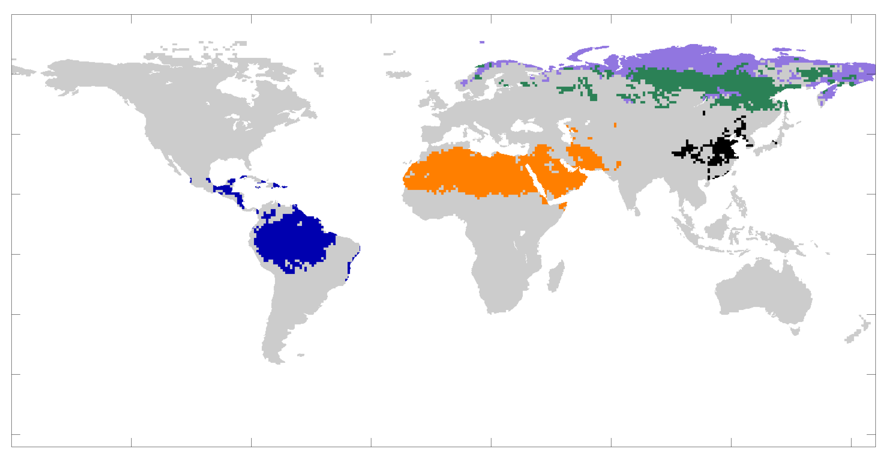
2.1. Land Cover Classification Data
2.2. AI-Based AOD
2.3. Other Satellite-Based AOD Data
2.4. In Situ Data
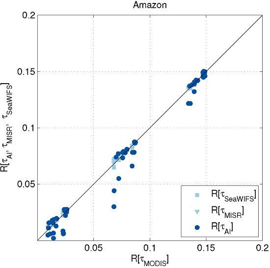
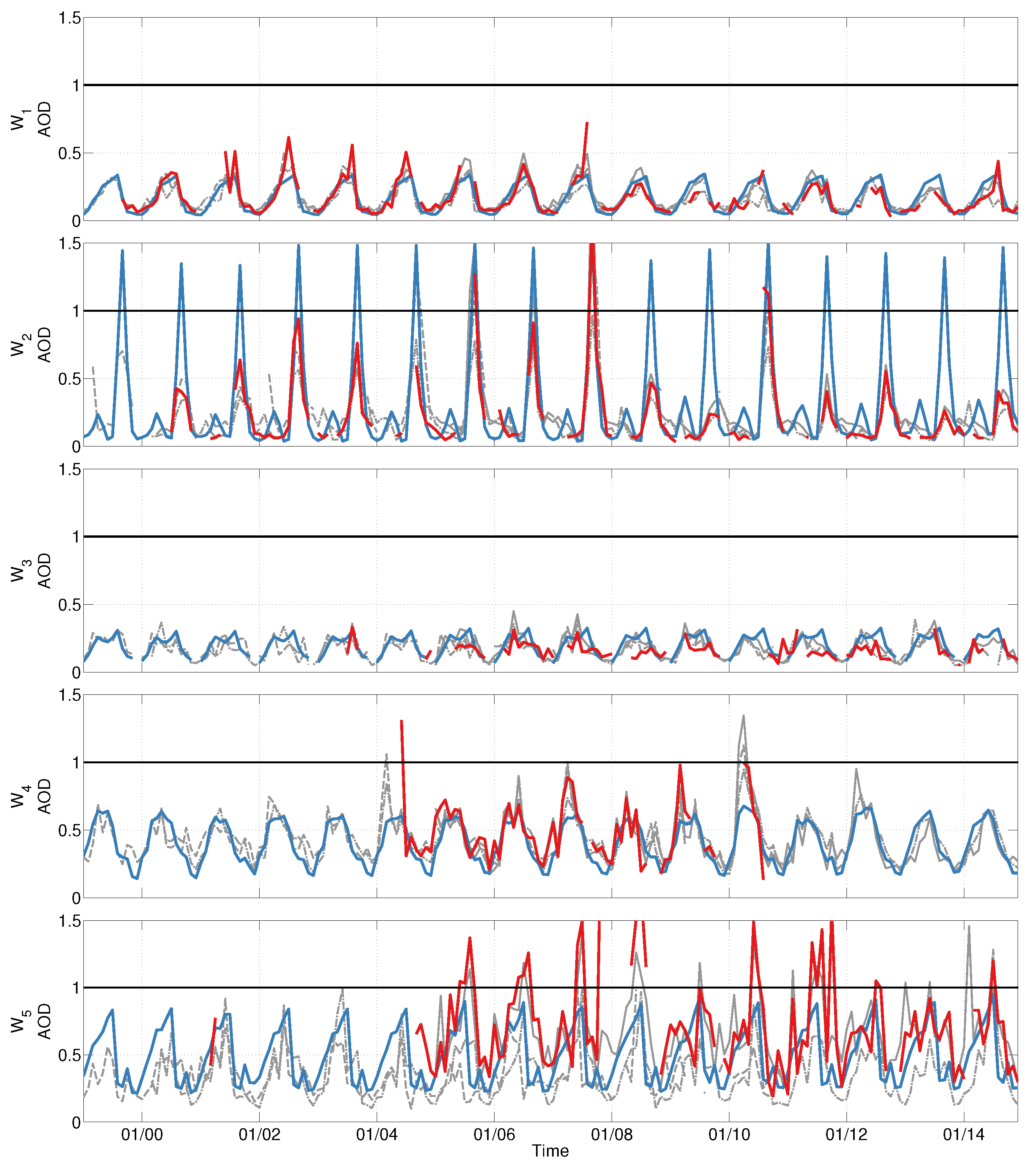
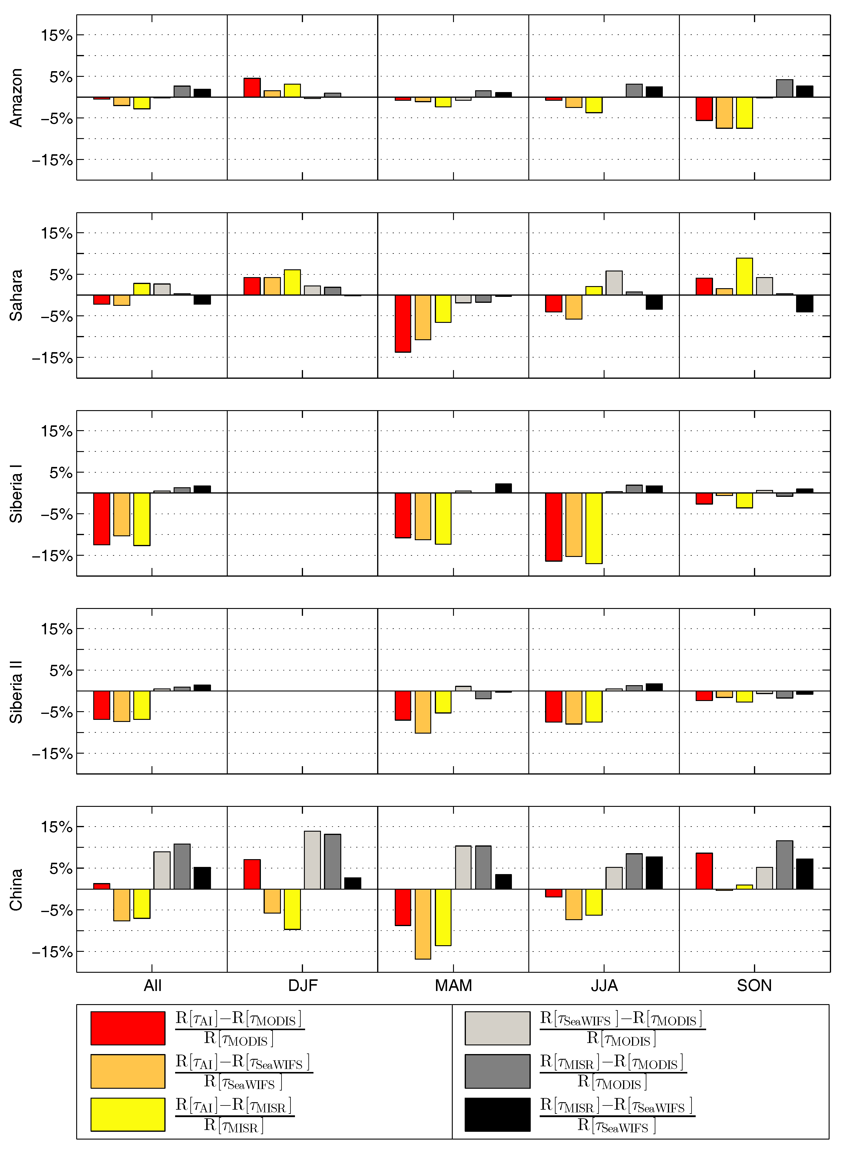
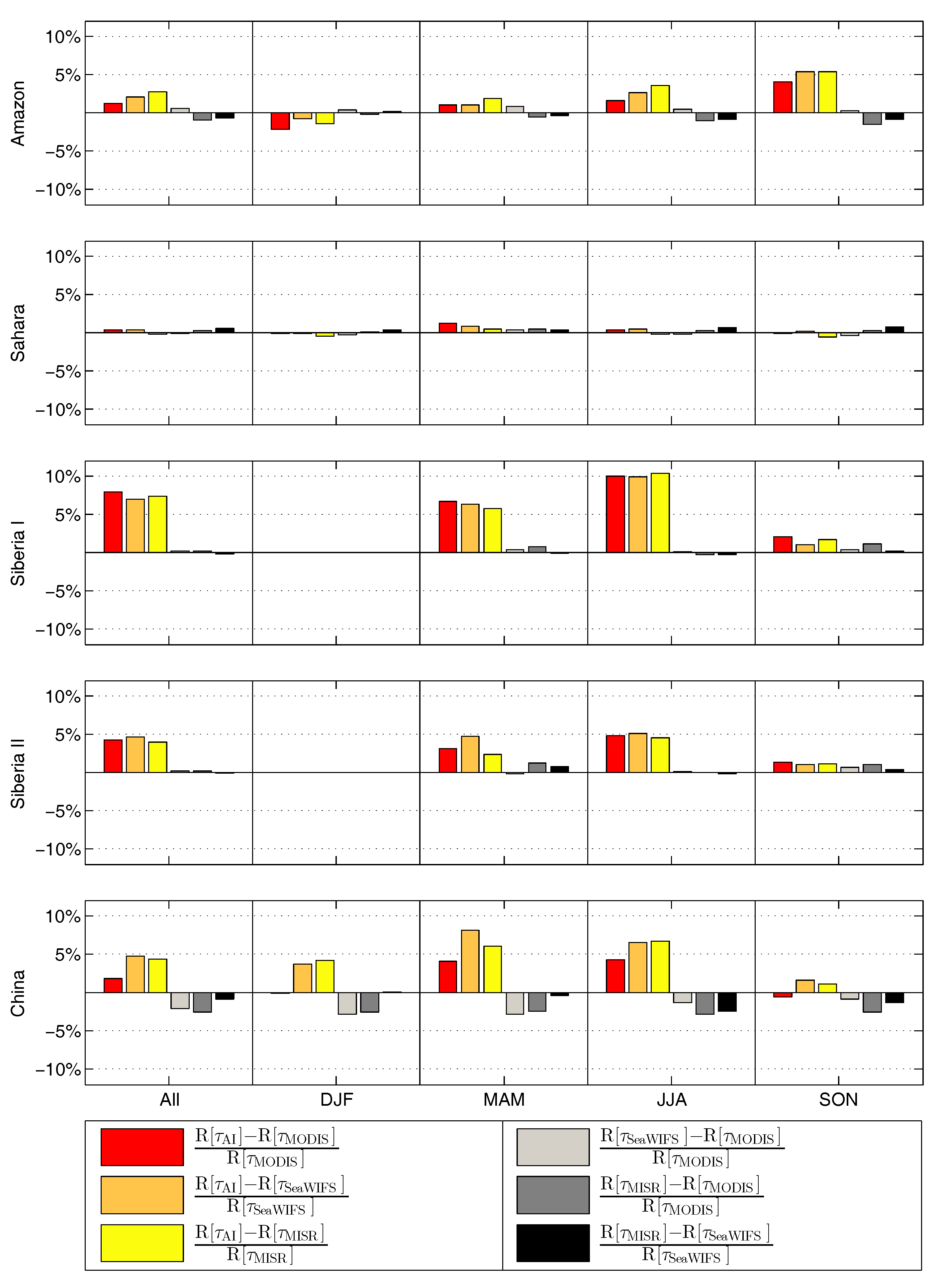
3. Comparison with In Situ Measurements
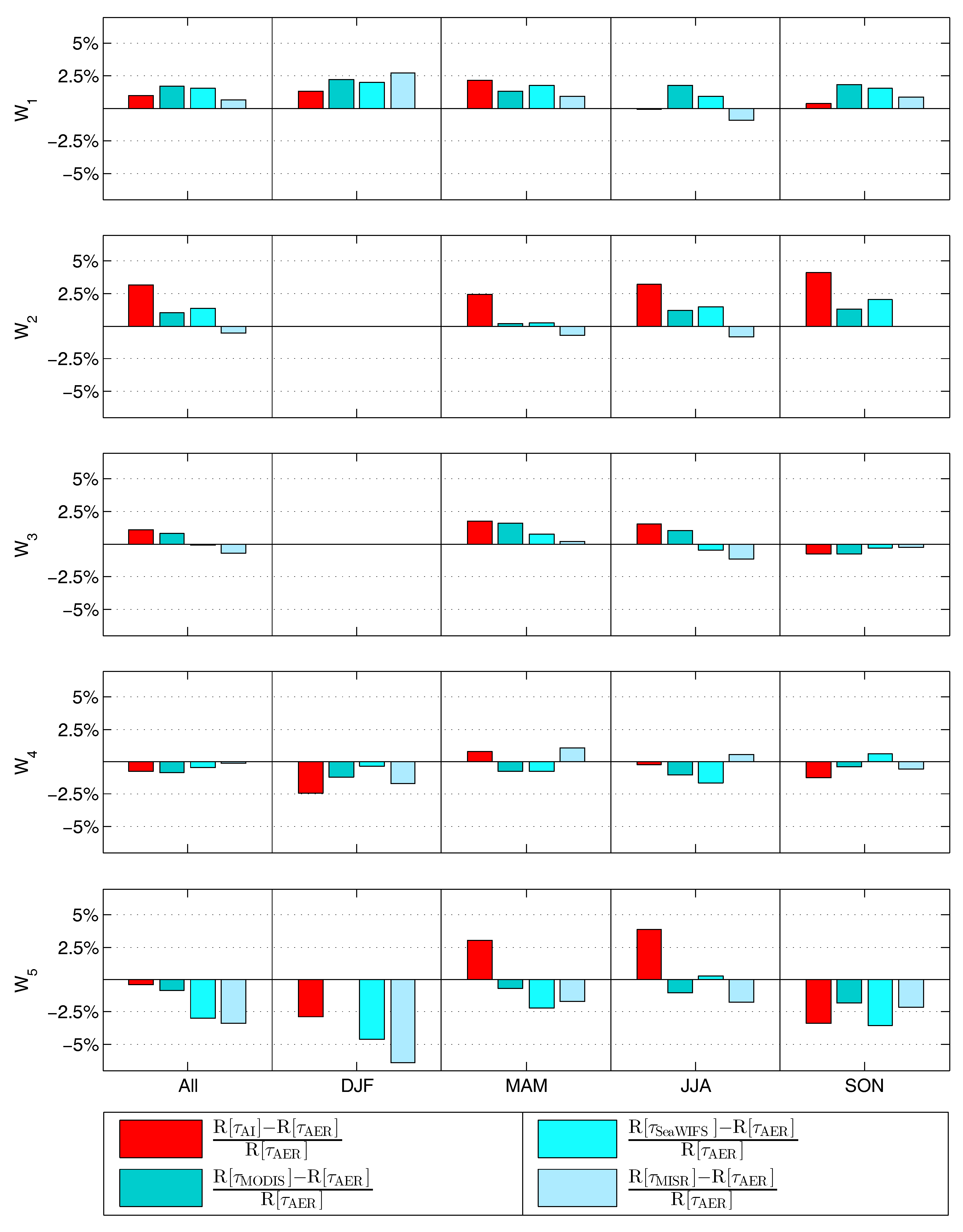
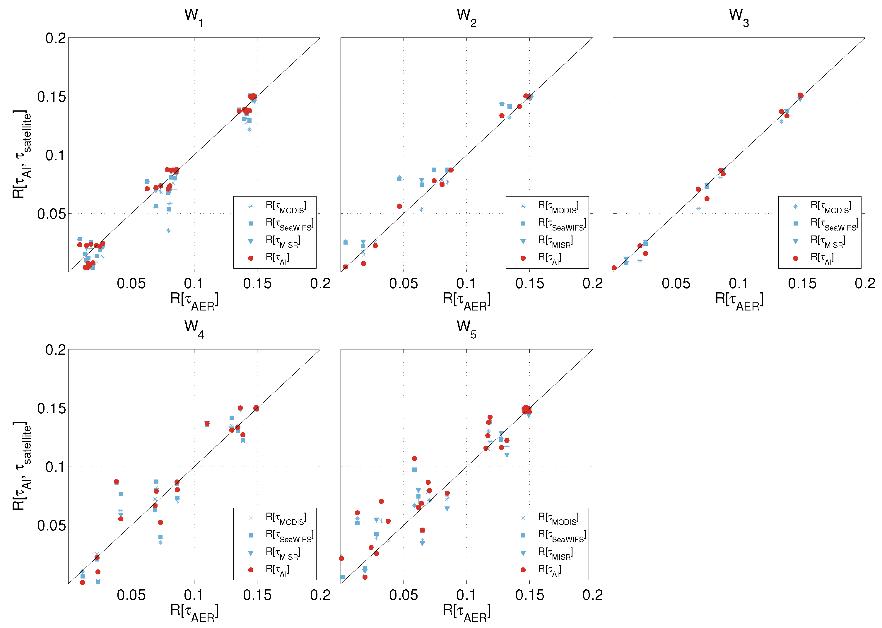
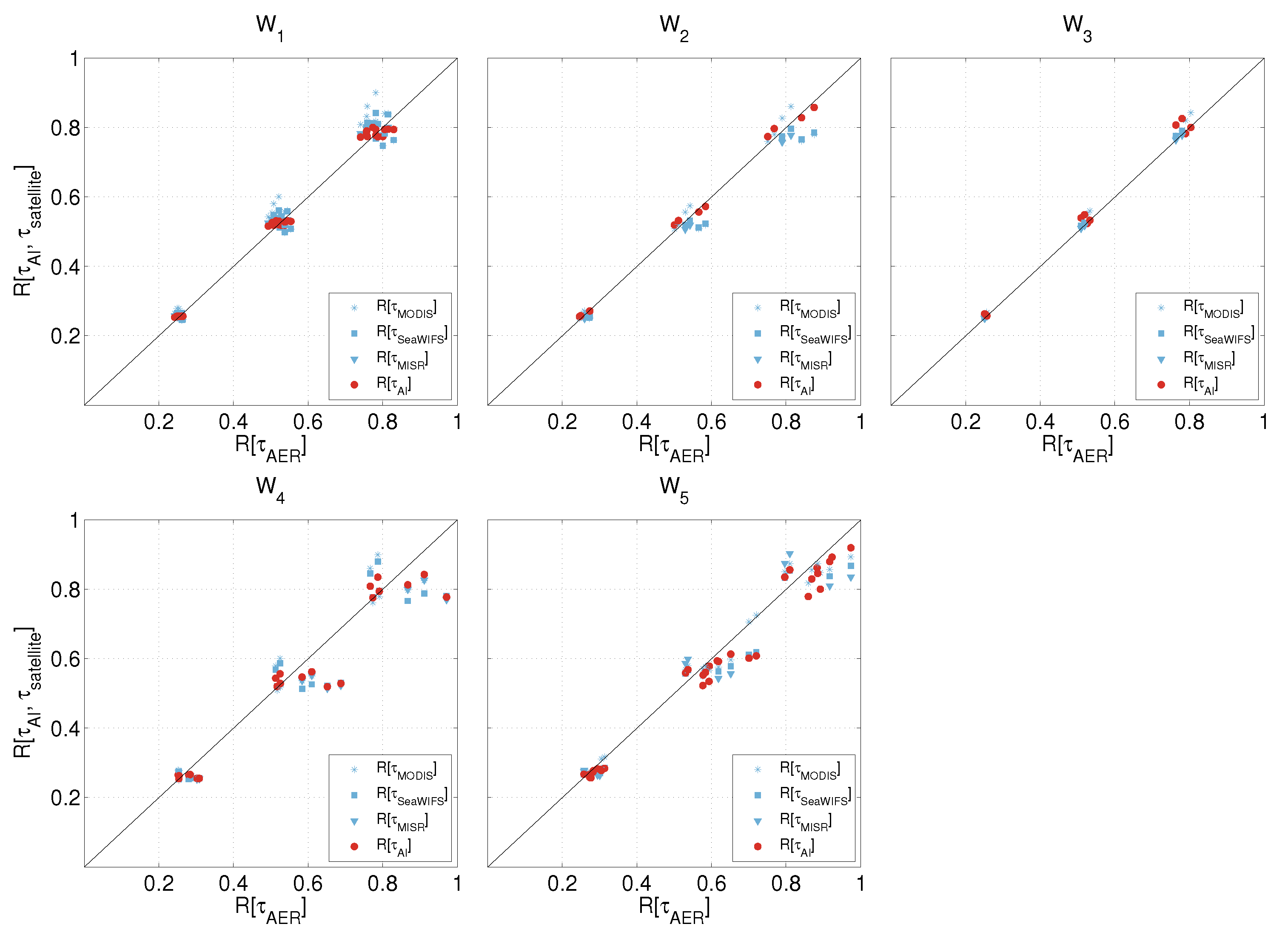
4. The Effect of AOD Estimate on Atmospheric Correction
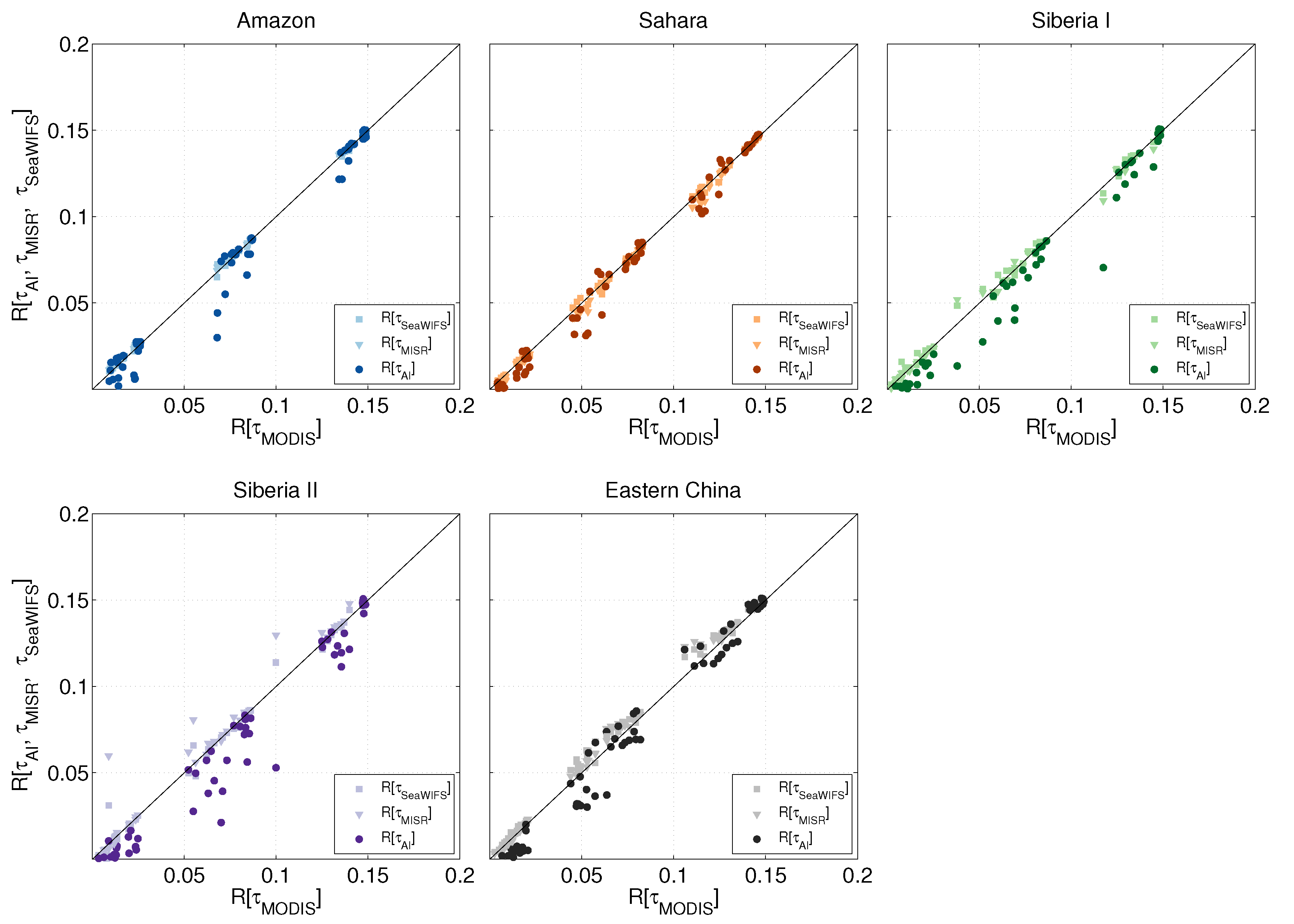
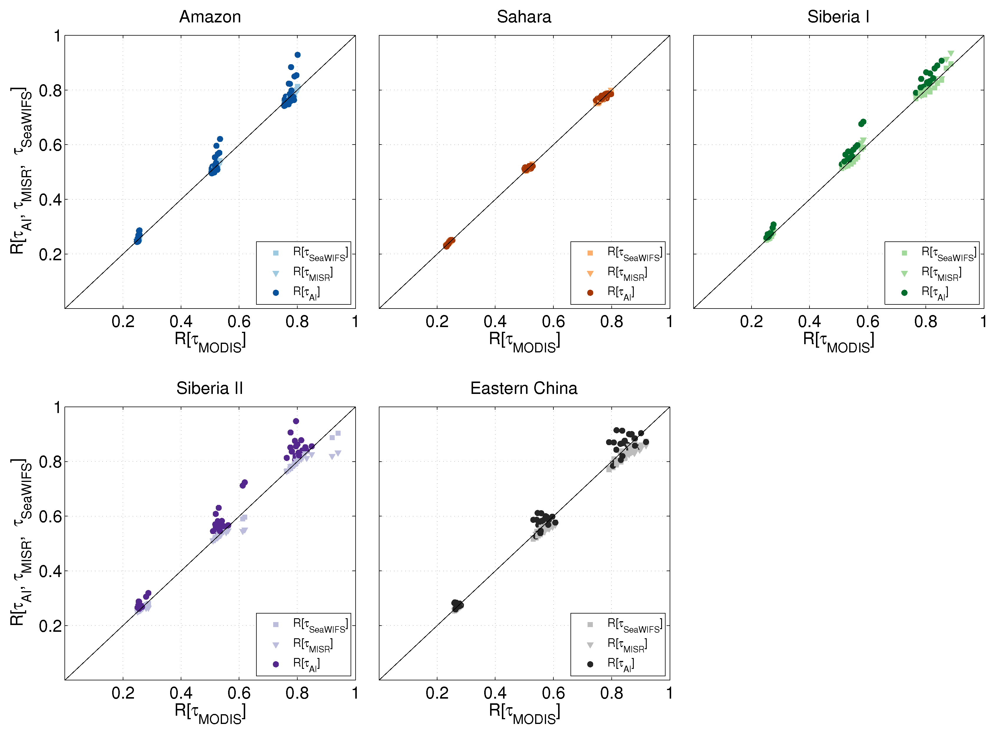
4.1. Satellite-Based AOD
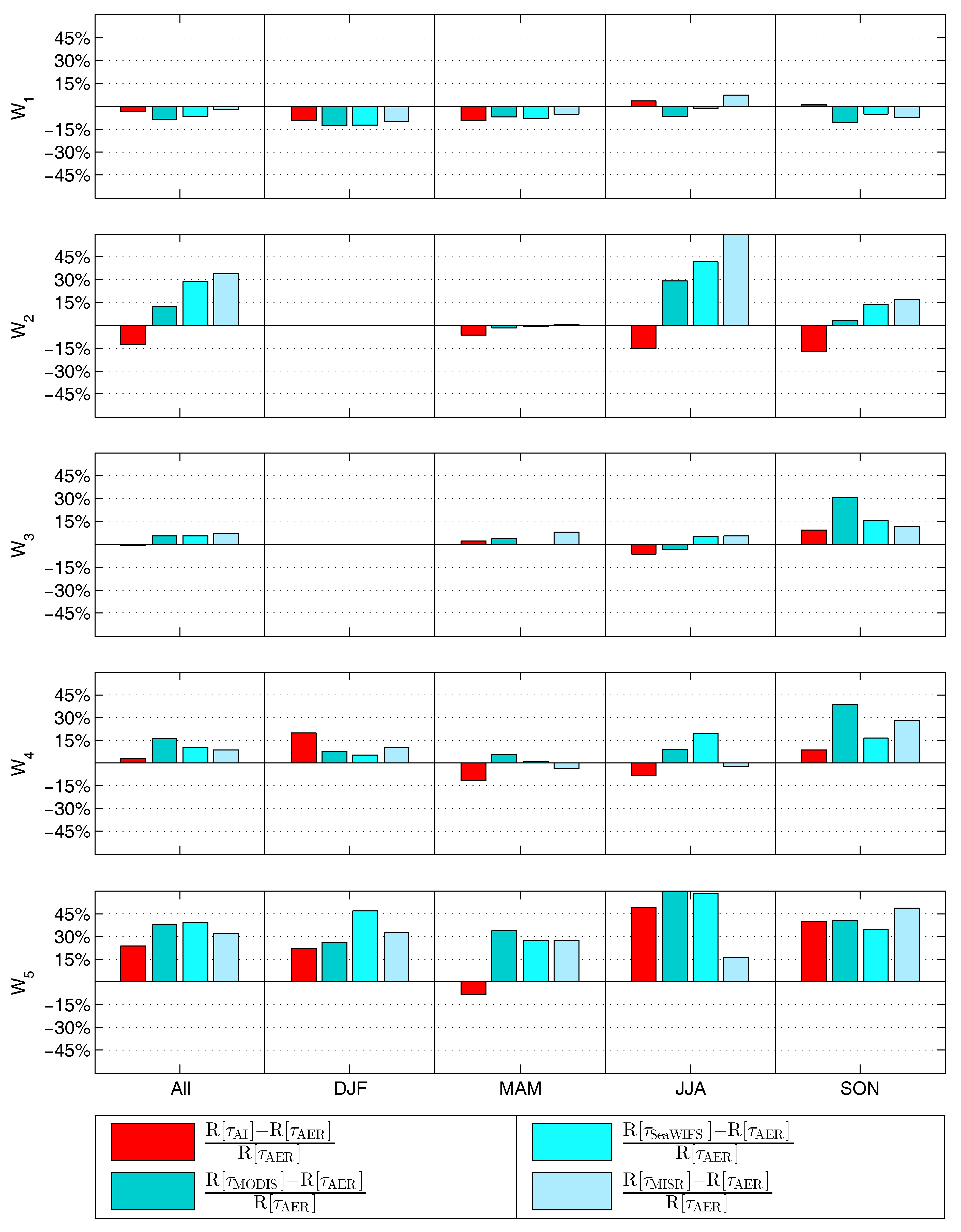
4.2. In Situ AOD
5. Conclusions
Acknowledgments
Author Contributions
Conflicts of Interest
Abbreviations
| AOD | Aerosol Optical Depth |
| AI | Aerosol Index |
| SZA | Solar Zenith Angle |
| TOA | Top Of Atmosphere |
| constructed AOD time series 1982–2014 | |
| AOD retrieved from MODIS observations | |
| AOD retrieved from MISR observations | |
| AOD retrieved from SeaWIFS observations | |
| the mean value of calculated AOD values (from AERONET data) at 550 nm | |
| corresponds to the used AOD information | |
| R[] | a surface reflectance values calculated using SMAC |
| SMAC | a Simplified Method for Atmospheric Correction algorithm |
| DJF | December–January–February |
| MAM | March–April–May |
| JJA | June–July–August |
| SON | September–October–November |
| CLARA-Ax SAL | the Surface ALbedo from the CMSAF cLoud, Albedo and RAdiation data record, version x |
References
- World Meteorological Organization. The Global Observing System for Climate: Implementation Needs. 2006. Available online: https://library.wmo.int/opac/doc_num.php?explnum_id=3417 (accessed on 2 October 2017).
- Riihelä, A.; Manninen, T.; Laine, V. Observed changes in the albedo of the Arctic sea-ice zone for the period 1982–2009. Nat. Clim. Chang. 2013, 3, 895–898. [Google Scholar] [CrossRef]
- Hsu, N.C.; Herman, J.R.; Torres, O.; Holben, B.N.; Tanré, D.; Eck, T.F.; Smirnov, A.; Chatenet, B.; Lavenu, F. Comparisons of the TOMS aerosol index with Sun-photometer aerosol optical thickness: Results and applications. J. Geophys. Res. 1999, 104, 6269–6279. [Google Scholar] [CrossRef]
- Torres, O.; Bhartia, P.K.; Herman, J.R.; Sinyuk, A.; Ginoux, P.; Holben, B. A long-term record of aerosol optical depth from TOMS observations and comparison to AERONET measurements. J. Atmos. Sci. 2002, 59, 398–413. [Google Scholar] [CrossRef]
- Karlsson, K.-G.; Anttila, K.; Trentmann, J.; Stengel, M.; Fokke Meirink, J.; Devasthale, A.; Hanschmann, T.; Kothe, S.; Jääskeläinen, E.; Sedlar, J.; et al. CLARA-A2: The second edition of the CM SAF cloud and radiation data record from 34 years of global AVHRR data. Atmos. Chem. Phys. 2017, 17, 5809–5828. [Google Scholar] [CrossRef]
- Schulz, J.; Albert, P.; Behr, H.-D.; Caprion, D.; Deneke, H.; Dewitte, S.; Dürr, B.; Fuchs, P.; Gratzki, A.; Hechler, P.; et al. Operational climate monitoring from space: The EUMETSAT Satellite Application Facility on Climate Monitoring (CM-SAF). Atmos. Chem. Phys. 2009, 9, 1687–1709. Available online: http://www.cmsaf.eu/EN/Home/home_node.html (accessed on 2 October 2017). [CrossRef]
- Rahman, H.; Dedieu, G. SMAC: A simplified method for the atmospheric correction of satellite measurements in the solar spectrum. Int. J. Remote Sens. 1994, 15, 123–143. [Google Scholar] [CrossRef]
- Jääskeläinen, E.; Manninen, T.; Tamminen, J.; Laine, M. Method for Constructing an AOD Related Atmospheric Correction Time Series for CLARA-A2 SAL Data Record. FMI Reports. 2017. Available online: https://helda.helsinki.fi/handle/10138/224308 (accessed on 2 October 2017).
- Herman, J.R.; Bhartia, P.K.; Torres, O.; Hsu, C.; Seftor, C.; Celarier, E. Global distribution of UV-absorbing aerosols from nimbus-7/TOMS data. J. Geophys. Res. 1997, 102, 16911–16922. [Google Scholar] [CrossRef]
- Hansen, M.; DeFries, R.; Townshend, J.R.G.; Sohlberg, R. UMD Global Land Cover Classification, 1 Degree, 1.0. Department of Geography, University of Maryland: College Park, Maryland, 1981–1994; Available online: http://glcf.umd.edu/data/landcover/ (accessed on 2 October 2017).
- European Commision Joint Research Centre. The Global Land Cover Map for the Year 2000, 2003. GLC2000 Database. Available online: http://forobs.jrc.ec.europa.eu/products/glc2000/products.php (accessed on 2 October 2017).
- Stein-Zweers, D.; Veefkind, P. OMI/Aura Multi-Wavelength Aerosol Optical Depth and Single Scattering Albedo L3 1 Day Best Pixel in 0.25 Degree × 0.25 Degree V3. 2002. Available online: http://dx.doi.org/10.5067/Aura/OMI/DATA3004 (accessed on 2 October 2017).
- TOMS Science Team. TOMS/Nimbus-7 Total Ozone Aerosol Index UV-Reflectivity UV-B Erythemal Irradiances Daily L3 Global 1×1.25 deg V008. Available online: http://disc.sci.gsfc.nasa.gov/datacollection/TOMSN7L3_V008.html (accessed on 2 October 2017).
- TOMS Science Team. TOMS Earth-Probe Total Ozone (O3) Aerosol Index UV-Reflectivity UV-B Erythemal Irradiance Daily L3 Global 1 deg×1.25 deg V008. Available online: https://disc.gsfc.nasa.gov/datacollection/TOMSEPL3_008.html (accessed on 2 October 2017).
- Hubanks, P.; Platnick, S.; King, M.; Ridgway, B. MODIS Atmosphere L3 Gridded Product Algorithm Theoretical Basis Document for C6. 2015. Available online: http://modis-atmos.gsfc.nasa.gov/_docs/L3_ATBD_C6.pdf (accessed on 2 October 2017).
- Platnick, S. MODIS Atmosphere L3 Daily Product. 2015. Available online: http://dx.doi.org/10.5067/MODIS/MYD08_D3.006 (accessed on 29 June 2017).
- Kaufman, Y.J.; Tanré, D.; Remer, L.A.; Vermote, E.F.; Chu, A.; Holben, B.N. Operational remote sensing of tropospheric aerosol over land from EOS moderate resolution imaging spectroradiometer. J. Geophys. Res. 1997, 102, 17051–17067. [Google Scholar] [CrossRef]
- Levy, R.C.; Remer, L.A.; Mattoo, S.; Vermote, E.F.; Kaufman, Y.J. Second-generation operational algorithm: Retrieval of aerosol properties over land from inversion of Moderate Resolution Imaging Spectroradiometer spectral reflectance. J. Geophys. Res. 2007, 112. [Google Scholar] [CrossRef]
- Levy, R.C.; Remer, L.A.; Kleidman, R.G.; Mattoo, S.; Ichoku, C.; Kahn, R.; Eck, T.F. Global evaluation of the Collection 5 MODIS dark-target aerosol products over land. Atmos. Chem. Phys. 2010, 10, 10399–10420. [Google Scholar] [CrossRef] [Green Version]
- Remer, L.A.; Kaufman, Y.J.; Tanré, D.; Mattoo, S.; Chu, D.A.; Martins, J.V.; Li, R.R.; Ichoku, C.; Levy, R.C.; Kleidman, R.G.; et al. The MODIS aerosol algorithm, products, and validation. J. Atmos. Sci. 2005, 62, 947–973. [Google Scholar] [CrossRef]
- Hsu, N.C.; Tsay, S.; King, M.D.; Herman, J.R. Aerosol properties over bright-reflecting source regions. IEEE Trans. Geosci. Remote Sens. 2004, 42, 557–569. [Google Scholar] [CrossRef]
- Hsu, N.C.; Jeong, M.-J.; Bettenhausen, C.; Sayer, A.M.; Hansell, R.; Seftor, C.S.; Huang, J.; Tsay, S.C. Enhanced deep blue aerosol retrieval algorithm: The 2nd Generation. J. Geophys. Res. 2013, 118, 1–20. [Google Scholar] [CrossRef]
- MISR Science Team. Terra/MISR Level 3, Component Global Aerosol Daily, Version 4. 2015. Available online: http://dx.doi.org/10.5067/Terra/MISR/MIL3DAE_L3.004 (accessed on 2 October 2017).
- Sayer, A.; Hsu, N.C.; Bettenhausen, C.; Jeong, M.J.; Holben, B.N.; Zhang, J. Global and regional evaluation of over-land spectral aerosol optical depth retrievals from SeaWiFS. Atmos. Meas. Tech. 2012, 5, 1761–1778. [Google Scholar] [CrossRef]
- Hsu, N.C.; Sayer, A.M.; Jeong, M.-J.; Bettenhausen, C. SeaWiFS Deep Blue Aerosol Optical Depth and Angstrom Exponent Daily Level 3 Data Gridded at 0.5 Degrees V004. 2013. Available online: http://dx.doi.org/10.5067/MEASURES/SWDB/DATA301 (accessed on 2 October 2017).
- Aerosol Robotic Network (AERONET) Homepage. Available online: https://aeronet.gsfc.nasa.gov/ (accessed on 25 October 2017).
- Holben, B.N.; Eck, T.F.; Slutsker, I.; Tanr, D.; Buis, J.P.; Setzer, A.; Vermote, E.; Reagan, J.A.; Kaufman, Y.J.; Nakajima, T.; et al. AERONET—Federated instrument network and data archive for aerosol characterization. Remote Sens. Environ. 1998, 66, 1–16. [Google Scholar] [CrossRef]
- Clark, R.N.; Swayze, G.A.; Wise, R.; Livo, E.; Hoefen, T.; Kokaly, R.; Sutley, S.J. USGS Digital Spectral Library Splib06a: US Geological Survey. Digital Data Series 231; 2007. Available online: http://speclab.cr.usgs.gov/spectral.lib06 (accessed on 2 October 2017).


| Satellite | Product | Version | Period | L3 Resolution | |
|---|---|---|---|---|---|
| AOD | |||||
| - | - | v1.0 | January 1982–December 2014 | 0.25 0.25 | |
| MISR | Terra | MIL3DAE | V4 | February 2000–December 2014 | 0.50 0.50 |
| MODIS | Aqua | MYD08 | 006 | January 2005–December 2014 | 1.00 1.00 |
| SeaWIFS | SeaStar | SWDB_L305 | v004 | September 1997–December 2010 | 0.50 0.50 |
| AERONET | - | - | v3 | 1999–2014 | - |
| LUC | |||||
| AVHRR | - | UMD Global Land | - | 1981–1994 | 1.00 1.00 |
| Cover Classification | |||||
| VEGETATION | SPOT 4 | GLC2000 | - | 2000 | 0.01 0.01 |
| Name | (Lat, Long) | LUC | Period | |
|---|---|---|---|---|
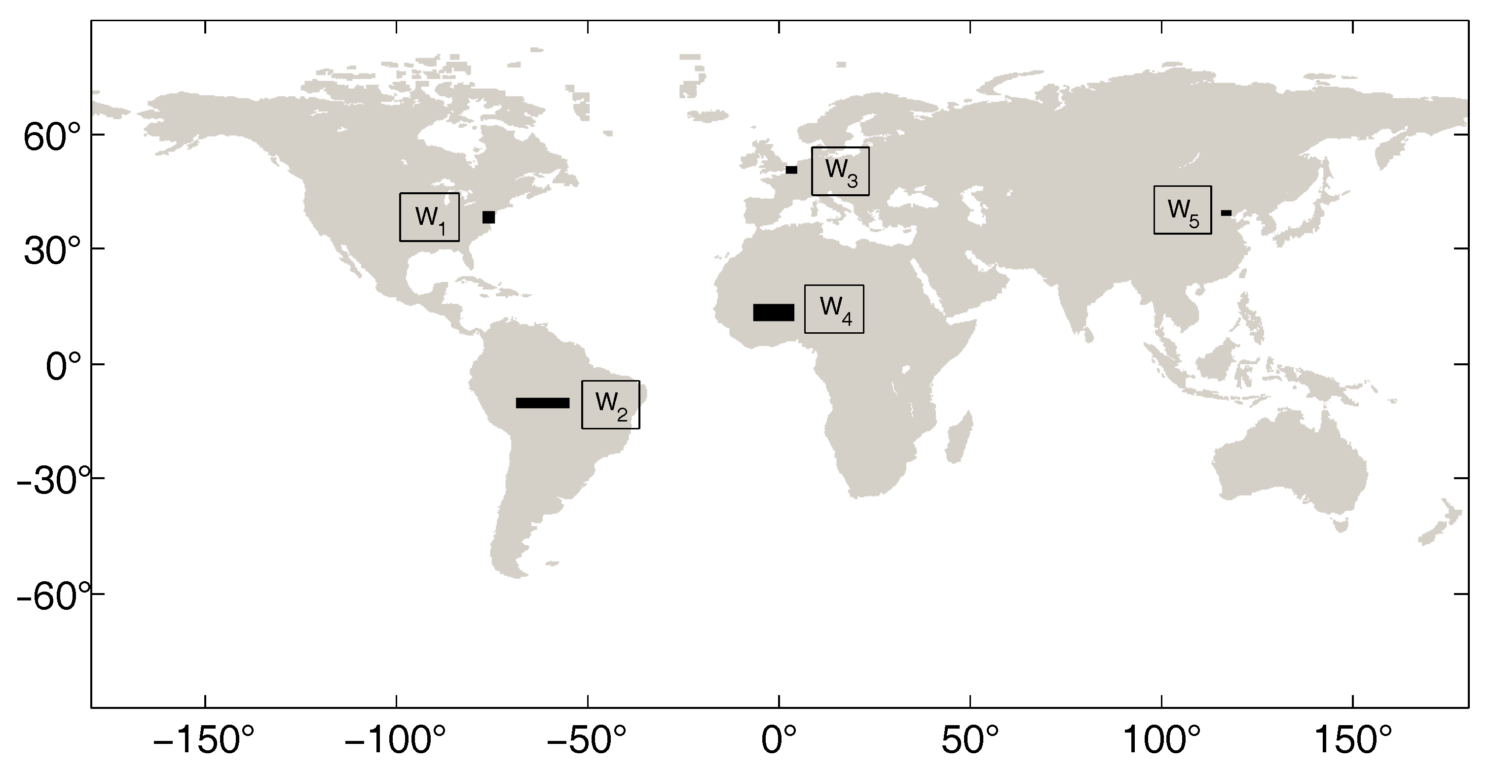
| W | GSFC | (38.99, −76.83) | wooded grassland | 1999–2014 |
| MD Science Center | (37.94, −75.48) | mixed coniferous forest and woodland | 1999–2014 | |
| Wallops | (39.28, −76.62) | wooded grassland | 1999–2014 | |
| W | Alta Floresta | (−9.87, −56.10) | broadleaf evergreen forest | 1999–2013 |
| Rio Branco | (−9.96, −67.87) | broadleaf evergreen forest | 2000–2013 | |
| W | Dunkerque | (51.04, 2.37) | cultivated crops | 2003–2014 |
| Lille | (50.61, 3.14) | wooded grassland | 1999–2014 | |
| Oostende | (51.23, 2.93) | cultivated crops | 2001–2014 | |
| W | Agoufou | (15.35, −1.48) | grassland | 2002–2011 |
| Banizoumbou | (13.54, 2.66) | shrubs and bare ground | 1999–2011 | |
| IER Cinzana | (13.28, −5.93) | grassland | 2004–2011 | |
| W | Beijing | (39.98, 116.38) | broadleaf decidious forest and woodland | 2001–2014 |
| XiangHe | (39.75, 116.96) | broadleaf decidious forest and woodland | 2001, 2004–2014 |
| – | – | – | – | |
|---|---|---|---|---|
| W | 0.00 | 0.03 | 0.00 | −0.02 |
| W | 0.15 | 0.06 | 0.06 | −0.02 |
| W | 0.05 | 0.03 | 0.03 | 0.00 |
| W | −0.08 | −0.01 | −0.02 | −0.04 |
| W | −0.22 | −0.06 | −0.39 | −0.35 |
© 2017 by the authors. Licensee MDPI, Basel, Switzerland. This article is an open access article distributed under the terms and conditions of the Creative Commons Attribution (CC BY) license (http://creativecommons.org/licenses/by/4.0/).
Share and Cite
Jääskeläinen, E.; Manninen, T.; Tamminen, J.; Laine, M. The Aerosol Index and Land Cover Class Based Atmospheric Correction Aerosol Optical Depth Time Series 1982–2014 for the SMAC Algorithm. Remote Sens. 2017, 9, 1095. https://doi.org/10.3390/rs9111095
Jääskeläinen E, Manninen T, Tamminen J, Laine M. The Aerosol Index and Land Cover Class Based Atmospheric Correction Aerosol Optical Depth Time Series 1982–2014 for the SMAC Algorithm. Remote Sensing. 2017; 9(11):1095. https://doi.org/10.3390/rs9111095
Chicago/Turabian StyleJääskeläinen, Emmihenna, Terhikki Manninen, Johanna Tamminen, and Marko Laine. 2017. "The Aerosol Index and Land Cover Class Based Atmospheric Correction Aerosol Optical Depth Time Series 1982–2014 for the SMAC Algorithm" Remote Sensing 9, no. 11: 1095. https://doi.org/10.3390/rs9111095