Airborne LiDAR Data Filtering Based on Geodesic Transformations of Mathematical Morphology

 , and
, and
Abstract
:
1. Introduction
2. Methodology
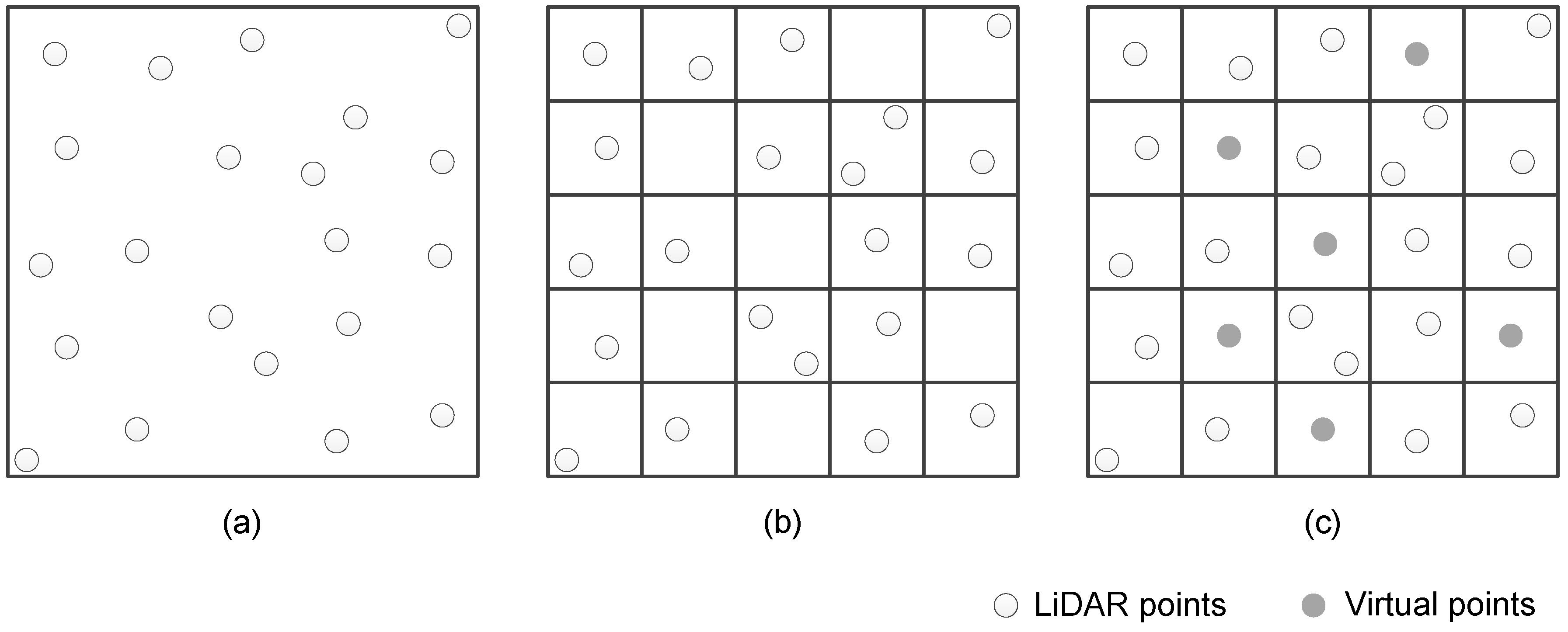
2.1. Reorganizing Data and Removing Low Outliers
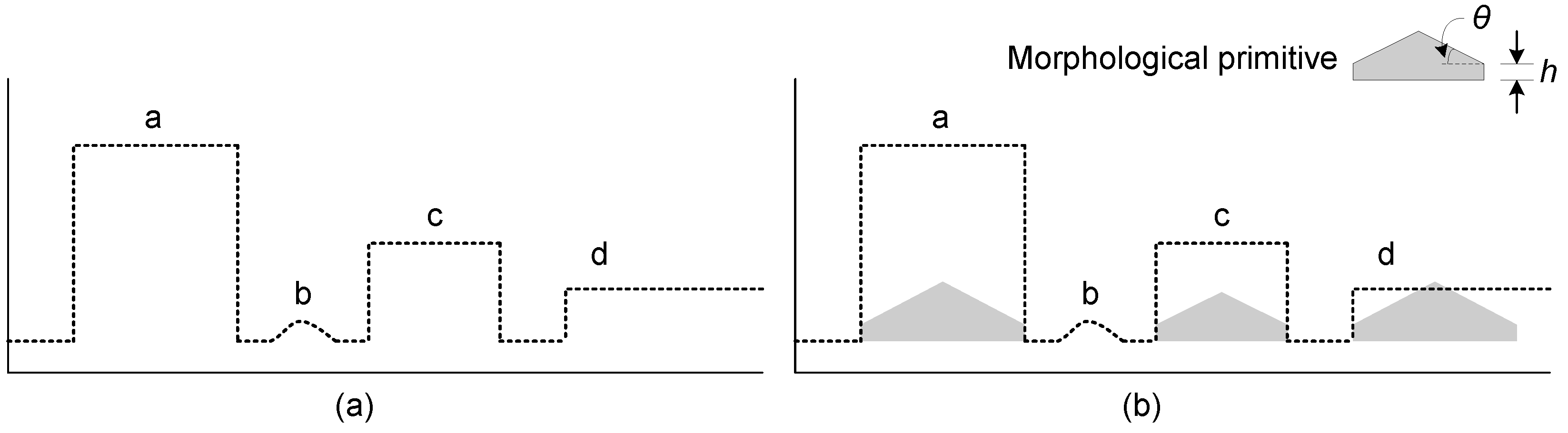
2.2. Calculating Morphological Gradients
2.3. Filtering Point Clouds by Geodesic Transformations
2.4. Experimental Approach
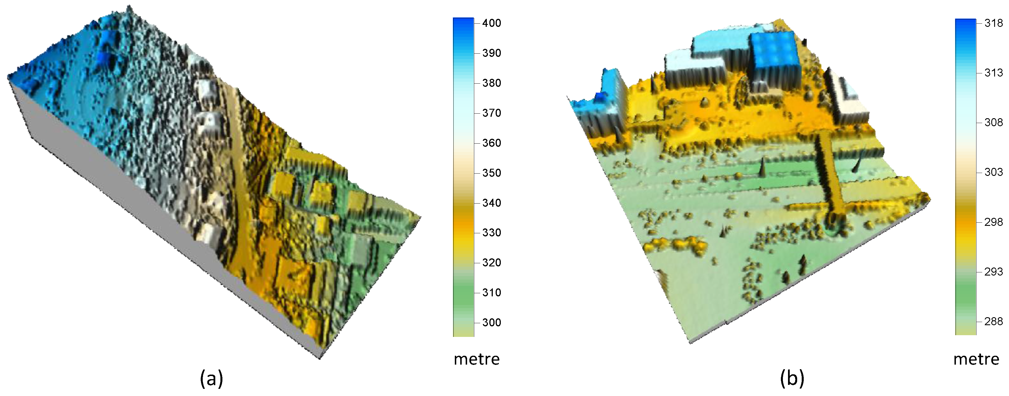
2.4.1. Test Data
2.4.2. Parameter Setting
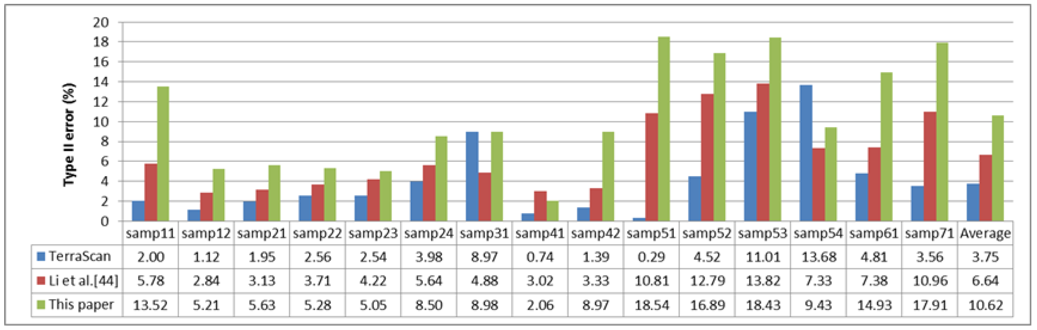
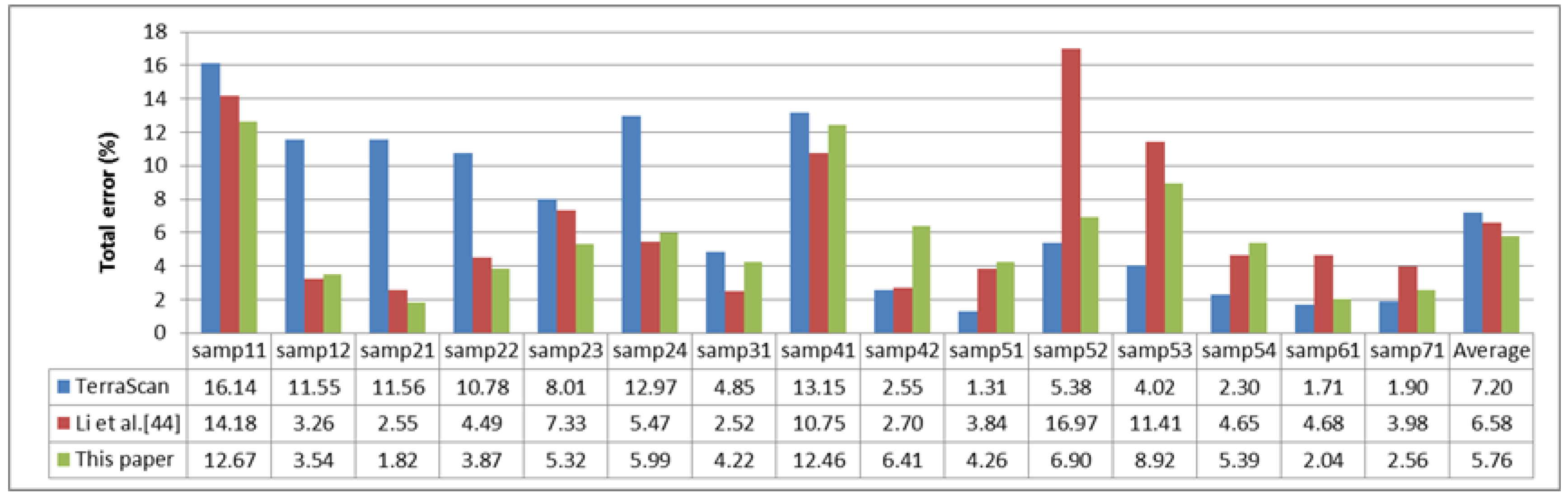
2.4.3. Evaluation Method
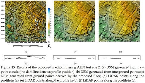
3. Results and Discussion
4. Conclusions
Acknowledgments
Author Contributions
Conflicts of Interest
References
- Meng, X.; Wang, L.; Silvan-Cardenas, J.L.; Currit, N. A multi-directional ground filtering algorithm for airborne lidar. ISPRS J. Photogramm. Remote Sens. 2009, 64, 117–124. [Google Scholar] [CrossRef]
- Shan, J.; Sampath, A. Urban dem generation from raw lidar data: A labeling algorithm and its performance. Photogramm. Eng. Remote Sens. 2005, 71, 217–226. [Google Scholar] [CrossRef]
- Filin, S.; Pfeifer, N. Segmentation of airborne laser scanning data using a slope adaptive neighborhood. ISPRS J. Photogramm. Remote Sens. 2006, 60, 71–80. [Google Scholar] [CrossRef]
- Zeng, Z.; Wan, J.; Liu, H. An entropy-based filtering approach for airborne laser scanning data. Infrared Phys. Technol. 2016, 75, 87–92. [Google Scholar] [CrossRef]
- Sirmacek, B.; Taubenbock, H.; Reinartz, P.; Ehlers, M. Performance evaluation for 3-d city model generation of six different dsms from air-and spaceborne sensors. IEEE J. Sel. Top. Appl. Earth Obs. Remote Sens. 2012, 5, 59–70. [Google Scholar] [CrossRef]
- White, S.A.; Wang, Y. Utilizing dems derived from lidar data to analyze morphologic change in the north carolina coastline. Remote Sens. Environ. 2003, 85, 39–47. [Google Scholar] [CrossRef]
- Stoker, J.M.; Greenlee, S.K.; Gesch, D.B.; Menig, J.C. Click: The new usgs center for lidar information coordination and knowledge. Photogramm. Eng. Remote Sens. 2006, 72, 613–616. [Google Scholar]
- Zhang, K.; Chen, S.C.; Whitman, D.; Shyu, M.L.; Yan, J.; Zhang, C. A progressive morphological filter for removing nonground measurements from airborne lidar data. IEEE Trans. Geosci. Remote Sens. 2003, 41, 872–882. [Google Scholar] [CrossRef]
- Sithole, G.; Vosselman, G. Experimental comparison of filter algorithms for bare-earth extraction from airborne laser scanning point clouds. ISPRS J. Photogramm. Remote Sens. 2004, 59, 85–101. [Google Scholar] [CrossRef]
- Nie, S.; Wang, C.; Dong, P.; Xi, X.; Luo, S.; Qin, H. A revised progressive tin densification for filtering airborne lidar data. Measurement 2017, 104, 70–77. [Google Scholar] [CrossRef]
- Shirowzhan, S.; Lim, S.; Trinder, J. Enhanced autocorrelation-based algorithms for filtering airborne lidar data over urban areas. J. Surv. Eng. 2015, 142, 04015008. [Google Scholar] [CrossRef]
- Zhao, X.; Guo, Q.; Su, Y.; Xue, B. Improved progressive tin densification filtering algorithm for airborne lidar data in forested areas. ISPRS J. Photogramm. Remote Sens. 2016, 117, 79–91. [Google Scholar] [CrossRef]
- Chen, Q.; Wang, H.; Zhang, H.; Sun, M.; Liu, X. A point cloud filtering approach to generating DTMs for steep mountainous areas and adjacent residential areas. Remote Sens. 2016, 8, 71. [Google Scholar] [CrossRef]
- Qin, L.; Wu, W.; Tian, Y.; Xu, W. Lidar filtering of urban areas with region growing based on moving-window weighted iterative least-squares fitting. IEEE Geosci. Remote Sens. Lett. 2017, 14, 841–845. [Google Scholar] [CrossRef]
- Yan, W.Y.; Shaker, A.; El-Ashmawy, N. Urban land cover classification using airborne lidar data: A review. Remote Sens. Environ. 2015, 158, 295–310. [Google Scholar] [CrossRef]
- Hui, Z.; Hu, Y.; Yevenyo, Y.Z.; Yu, X. An improved morphological algorithm for filtering airborne lidar point cloud based on multi-level kriging interpolation. Remote Sens. 2016, 8, 35. [Google Scholar] [CrossRef]
- Bartels, M.; Wei, H. Threshold-free object and ground point separation in lidar data. Pattern Recognit. Lett. 2010, 31, 1089–1099. [Google Scholar] [CrossRef]
- Silvan-Cardenas, J.L.; Wang, L. A multi-resolution approach for filtering lidar altimetry data. ISPRS J. Photogramm. Remote Sens. 2006, 61, 11–22. [Google Scholar] [CrossRef]
- Li, Y.; Yong, B.; Wu, H.; An, R.; Xu, H.; Xu, J.; He, Q. Filtering airborne lidar data by modified white top-hat transform with directional edge constraints. Photogramm. Eng. Remote Sens. 2014, 80, 133–141. [Google Scholar] [CrossRef]
- Chen, Q. Airborne lidar data processing and information extraction. Photogramm. Eng. Remote Sens. 2007, 73, 109–112. [Google Scholar]
- Zhang, J.; Lin, X. Filtering airborne lidar data by embedding smoothness-constrained segmentation in progressive tin densification. ISPRS J. Photogramm. Remote Sens. 2013, 81, 44–59. [Google Scholar] [CrossRef]
- Meng, X.; Currit, N.; Zhao, K. Ground filtering algorithms for airborne lidar data: A review of critical issues. Remote Sens. 2010, 2, 833–860. [Google Scholar] [CrossRef]
- Shan, J.; Toth, C.K. Topographic Laser Ranging and Scanning: Principles and Processing; CRC Press: Boca Raton, FL, USA, 2008. [Google Scholar]
- Vosselman, G. Slope based filtering of laser altimetry data. Int. Arch. Photogramm. Remote Sens. Spat. Inf. Sci. 2000, 33, 935–942. [Google Scholar]
- Sithole, G. Filtering of laser altimetry data using a slope adaptive filter. Int. Arch. Photogramm. Remote Sens. Spat. Inf. Sci. 2001, 34, 203–210. [Google Scholar]
- Wang, J.; Shan, J. Segmentation of Lidar Point Clouds for Building Extraction. In Proceedings of the ASPRS Annual Conference, Baltimore, MD, USA, 9–13 March 2009; ASPRS: Bethesda, MD, USA, 2009; pp. 9–13. [Google Scholar]
- Wang, C.; Tseng, Y. Dem generation from airborne lidar data by an adaptive dual-directional slope filter. Int. Arch. Photogramm. Remote Sens. Spat. Inf. Sci. 2010, 38, 628–632. [Google Scholar]
- Axelsson, P. Dem generation from laser scanner data using adaptive tin models. Int. Arch. Photogramm. Remote Sens. Spat. Inf. Sci. 2000, 33, 111–118. [Google Scholar]
- Axelsson, P. Processing of laser scanner data—Algorithms and applications. ISPRS J. Photogramm. Remote Sens. 1999, 54, 138–147. [Google Scholar] [CrossRef]
- Sohn, G.; Dowman, I. Terrain surface reconstruction by the use of tetrahedron model with the mdl criterion. Int. Arch. Photogramm. Remote Sens. Spat. Inf. Sci. 2002, 34, 336–344. [Google Scholar]
- Lee, H.S.; Younan, N.H. DTM extraction of lidar returns via adaptive processing. IEEE Trans. Geosci. Remote Sens. 2003, 41, 2063–2069. [Google Scholar] [CrossRef]
- Pfeifer, N.; Stadler, P.; Briese, C. Derivation of digital terrain models in the scop environment. In Proceedings of the OEEPE Workshop on Airborne Laser Scanning and Interferometric SAR for Detailed Digital Elevation Models, Stockholm, Sweden, 1–3 March 2001. [Google Scholar]
- Chen, Q.; Gong, P.; Baldocchi, D.; Xie, G. Filtering airborne laser scanning data with morphological methods. Photogramm. Eng. Remote Sens. 2007, 73, 175–185. [Google Scholar] [CrossRef]
- Wu, H.; Li, Y.; Li, J.; Gong, J. A two-step displacement correction algorithm for registration of lidar point clouds and aerial images without orientation parameters. Photogramm. Eng. Remote Sens. 2010, 76, 1135–1145. [Google Scholar] [CrossRef]
- Li, Y.; Wu, H.; Xu, H.; An, R.; Xu, J.; He, Q. A gradient-constrained morphological filtering algorithm for airborne lidar. Opt. Laser Technol. 2013, 54, 288–296. [Google Scholar] [CrossRef]
- Yang, B.; Huang, R.; Dong, Z.; Zang, Y.; Li, J. Two-step adaptive extraction method for ground points and breaklines from lidar point clouds. ISPRS J. Photogramm. Remote Sens. 2016, 119, 373–389. [Google Scholar] [CrossRef]
- Chen, C.; Li, Y.; Yan, C.; Dai, H.; Liu, G.; Guo, J. An improved multi-resolution hierarchical classification method based on robust segmentation for filtering ALs point clouds. Int. J. Remote Sens. 2016, 37, 950–968. [Google Scholar] [CrossRef]
- Arefi, H.; Hahn, M. A morphological reconstruction algorithm for separating off-terrain points from terrain points in laser scanning data. Int. Arch. Photogramm. Remote Sens. Spat. Inf. Sci. 2005, 36, 120–125. [Google Scholar]
- Kobler, A.; Pfeifer, N.; Ogrinc, P.; Todorovski, L.; Oštir, K.; Džeroski, S. Repetitive interpolation: A robust algorithm for DTM generation from aerial laser scanner data in forested terrain. Remote Sens. Environ. 2007, 108, 9–23. [Google Scholar] [CrossRef]
- Mongus, D.; Žalik, B. Parameter-free ground filtering of lidar data for automatic DTM generation. ISPRS J. Photogramm. Remote Sens. 2012, 67, 1–12. [Google Scholar] [CrossRef]
- Özcan, A.H.; Ünsalan, C. Lidar data filtering and DTM generation using empirical mode decomposition. IEEE J. Sel. Top. Appl. Earth Obs. Remote Sens. 2017, 10, 360–371. [Google Scholar] [CrossRef]
- Pingel, T.J.; Clarke, K.C.; McBride, W.A. An improved simple morphological filter for the terrain classification of airborne lidar data. ISPRS J. Photogramm. Remote Sens. 2013, 77, 21–30. [Google Scholar] [CrossRef]
- Soille, P. Morphological Image Analysis: Principles and Applications; Springer: New York, NY, USA, 2003. [Google Scholar]
- Li, Y.; Yong, B.; Wu, H.; An, R.; Xu, H. An improved top-hat filter with sloped brim for extracting ground points from airborne lidar point clouds. Remote Sens. 2014, 6, 12885–12908. [Google Scholar] [CrossRef]
- Mongus, D.; Zalik, B. Computationally efficient method for the generation of a digital terrain model from airborne lidar data using connected operators. IEEE J. Sel. Top. Appl. Earth Obs. Remote Sens. 2014, 7, 340–351. [Google Scholar] [CrossRef]
- Jahromi, A.B.; Zoej, M.J.V.; Mohammadzadeh, A.; Sadeghian, S. A novel filtering algorithm for bare-earth extraction from airborne laser scanning data using an artificial neural network. IEEE J. Sel. Top. Appl. Earth Obs. Remote Sens. 2011, 4, 836–843. [Google Scholar] [CrossRef]
- Susaki, J. Adaptive slope filtering of airborne lidar data in urban areas for digital terrain model (DTM) generation. Remote Sens. 2012, 4, 1804–1819. [Google Scholar] [CrossRef] [Green Version]
- Chen, C.; Li, Y.; Li, W.; Dai, H. A multiresolution hierarchical classification algorithm for filtering airborne lidar data. ISPRS J. Photogramm. Remote Sens. 2013, 82, 1–9. [Google Scholar] [CrossRef]


| Region | Point Spacing | Sample Data No. | Special Features |
|---|---|---|---|
| Urban | 1.0–1.5 m | 11, 12 | Steep slopes with mixture of buildings and vegetation on hillside, small objects |
| 21, 22, 23, 24 | Complex buildings, large buildings, roads with bridges, tunnel, data gaps, ramp, disconnected terrain | ||
| 31 | Densely distributed buildings and vegetation, building with irregular roof, mixture of low and high features, low point | ||
| 41, 42 | Elongated objects in railway station with sparse ground points, data gaps, low objects | ||
| Rural | 2.0–3.5 m | 51, 52, 53, 54 | Low vegetation on steep slopes, ridge, vegetation on river bank, data gaps, quarry with abrupt ground discontinuity, buildings of low resolution |
| 61 | Sharp ridge, ditches, data gaps | ||
| 71 | Bridge, road with embankments |
| Filtered | |||
|---|---|---|---|
| Ground Points | Object Points | ||
| Reference | Ground points | a | b |
| Object points | c | d | |
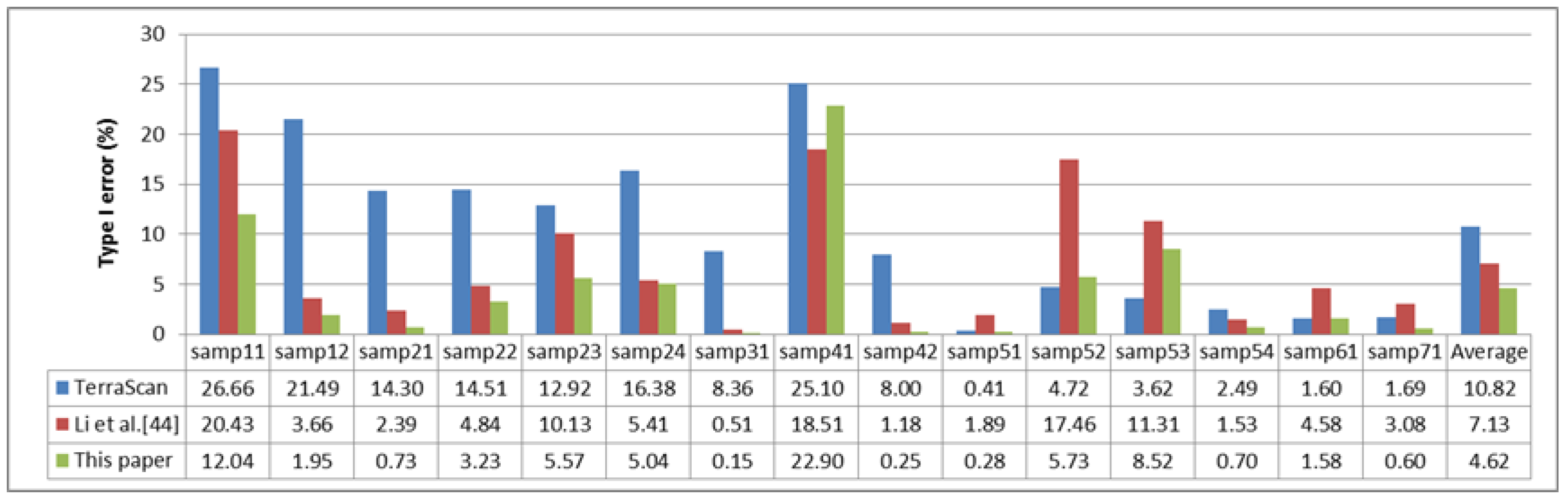
| Author | Type I Error (%) | Type II Error (%) | Total Error (%) |
|---|---|---|---|
| Jahromi et al. [46] | 11.00 | 3.47 | 7.70 |
| Chen et al. [48] | 4.49 | 5.63 | 4.11 |
| Susaki [47] | 6.70 | 11.26 | 7.39 |
| Pingel et al. [42] | 4.64 | 6.30 | 4.99 |
| Mongus and Zalik [40] | 3.49 | 9.39 | 5.62 |
| Zhang and Lin [21] | 13.11 | 10.19 | 10.63 |
| This paper | 4.62 | 10.62 | 5.76 |
© 2017 by the authors. Licensee MDPI, Basel, Switzerland. This article is an open access article distributed under the terms and conditions of the Creative Commons Attribution (CC BY) license (http://creativecommons.org/licenses/by/4.0/).
Share and Cite
Li, Y.; Yong, B.; Van Oosterom, P.; Lemmens, M.; Wu, H.; Ren, L.; Zheng, M.; Zhou, J. Airborne LiDAR Data Filtering Based on Geodesic Transformations of Mathematical Morphology. Remote Sens. 2017, 9, 1104. https://doi.org/10.3390/rs9111104
Li Y, Yong B, Van Oosterom P, Lemmens M, Wu H, Ren L, Zheng M, Zhou J. Airborne LiDAR Data Filtering Based on Geodesic Transformations of Mathematical Morphology. Remote Sensing. 2017; 9(11):1104. https://doi.org/10.3390/rs9111104
Chicago/Turabian StyleLi, Yong, Bin Yong, Peter Van Oosterom, Mathias Lemmens, Huayi Wu, Liliang Ren, Mingxue Zheng, and Jiajun Zhou. 2017. "Airborne LiDAR Data Filtering Based on Geodesic Transformations of Mathematical Morphology" Remote Sensing 9, no. 11: 1104. https://doi.org/10.3390/rs9111104