Nearest-Regularized Subspace Classification for PolSAR Imagery Using Polarimetric Feature Vector and Spatial Information

Abstract

Feature extraction using polarimetric synthetic aperture radar (PolSAR) images is of great interest in SAR classification, no matter if it is applied in an unsupervised approach or a supervised approach. In the supervised classification framework, a major group of methods is based on machine learning. Various machine learning methods have been investigated for PolSAR image classification, including neural network (NN), support vector machine (SVM), and so on. Recently, representation-based classifications have gained increasing attention in hyperspectral imagery, such as the newly-proposed sparse-representation classification (SRC) and nearest-regularized subspace (NRS). These classifiers provide excellent performance that is comparable to or even better than the classic SVM for remotely-sensed image processing. However, rare studies have been found to extend this representation-based NRS classification into PolSAR images. By the use of the NRS approach, a polarimetric feature vector-based PolSAR image classification method is proposed in this paper. The polarimetric SAR feature vector is constructed by the components of different target decomposition algorithms for each pixel, including those scattering components of Freeman, Huynen, Krogager, Yamaguchi decomposition, as well as the eigenvalues, eigenvectors and their consequential parameters such as entropy, anisotropy and mean scattering angle. Furthermore, because all these representation-based methods were originally designed to be pixel-wise classifiers, which only consider the separate pixel signature while ignoring the spatial-contextual information, the Markov random field (MRF) model is also introduced in our scheme. MRF can provide a basis for modeling contextual constraints. Two AIRSAR data in the Flevoland area are used to validate the proposed classification scheme. Experimental results demonstrate that the proposed method can reach an accuracy of around $99\%$ for both AIRSAR data by randomly selecting 300 pixels of each class as the training samples. Under the condition that the training data ratio is more than $4\%$, it has better performance than the SVM, SVM-MRF and NRS methods.

1. Introduction

Due to the active microwave imaging characteristics of fine resolution, day-and-night and weather-independence, Synthetic Aperture Radar (SAR) has been widely used for Earth remote sensing for more than 30 years, and it has come to play a significant role in geographical survey, climate change research, environment and Earth system monitoring, multi-dimensional mapping and other applications [1]. As the most essential properties of electromagnetic waves, polarization can reflect different information provided by the magnitude, frequency and phase. The polarization characteristics are highly related to the properties of the target, such as structure, size, posture, and so on. In the past few decades, many polarimetric SAR (PolSAR) systems (AIRSAR, ESAR, Pi-SAR, SAR580-Convair, ALOS2, RADARSAT-2, TerraSAR-X, etc.) have been developed and applied in land cover classification [2,3], soil moisture inversion [4,5,6,7], tomography retrieval [8], target detection [9,10], and so on. Because the orientation, size, dielectric and moisture characteristics of the target affect PolSAR data, the data are sensitive to the geometry of the building, branching structure and shape of the leaves [11,12]. Therefore, the PolSAR data classification has attracted extensive attention and become a hot topic in PolSAR applications [2,3,13,14,15,16,17].

Generally, the PolSAR classification mainly contains three steps, respectively polarimetric filtering, feature extraction and classification. The speckle reduction problem is more complicated for polarimetric SAR than a single polarization SAR, because of the difficulties of preserving polarimetric properties and of dealing with the cross-product terms [18]. In order to guarantee the posterior processing quality, various PolSAR filters are designed to reduce speckle and yield reliable results in practical PolSAR missions [19]. Although PolSAR can provide abundant target features within the structure, orientation and physical information, the measured data for each pixel are only comprised by a $2\times 2$ scattering matrix or a $3\times 3$ coherency matrix. How to map the limited scattering coefficients into diverse feature space, namely feature extraction, is still a difficult and challenged topic. In the early PolSAR classification methods, the backscattering coefficients and their ratios, differences are employed as the polarimetric features to represent object pixels. Though it is a most straightforward method, the physical mechanisms reflected by those features are composite and interdependent. The distinguishing nature of each object pixel is greatly reduced. Since target decomposition (TD) theorems were first formalized by Huynen [20], various TD methods were proposed to extract the independent components representing specific physical information to better characterize each pixel, such as Huynen decomposition [20], Freeman decomposition [21], van Zyl decomposition [22], Neumann decomposition [23], Krogager decomposition [24], Cloude–Pottier decomposition [25], Yamaguchi decomposition [26], Yang decomposition [27], Pauli decomposition [28], Barnes decomposition [29], and so on. According to those extracted features, the classifier is utilized to measure the similarity among pixels and realizes the category discrimination.

Recently, numerous supervised classification techniques for PolSAR imagery have been developed [11,30,31,32,33], providing excellent results in the discrimination of different land-cover objects. Among them, the most prominent is the representation-based classification [34]. In some cases, the representation-based classifications provide better performance than the classic neural network (NN) [35] and support vector method (SVM) [14] in that they require few labeled data instead of the traditional training-test mode. Representation-based classification is essentially based on the concept that a pixel can be represented as a linear combination of labeled samples via the sparse regularization methods, such as the $l_0$-norm, $l_1$-norm and $l_2$-norm regularization. In this manner, an approximation of the pixel is generated from labeled samples of each class independently, and the class label is then derived according to the class of the minimum representation error. Representation-based classification can be divided into two branches according to the methods for weight vector solving of the linear combination. One is by $l_2$-norm minimization, such as the nearest regularized subspace (NRS) [36,37] and the collaborative-representation classification (CRC) [38,39]; the other is by $l_0$ or $l_1$-norm minimization, such as the sparse representation-based classifier (SRC) [31,32,33].

Although all these aforementioned representation-based classifications demonstrate superior performance for high-dimensional data classification even with a limited number of training samples, they were originally designed to be pixel-wise classifiers, which only consider the polarimetric features while ignoring the spatial-contextual information (i.e., the correlations between spatially-adjacent pixels). For remote sensing imagery (whether optical or radar images), neighboring pixels tend to belong to the same class with high probability, thus spatial-contextual information should greatly increase the accuracy of the classification methods. Although wavelet transformation is a good way to extract texture feature including the polarimetric and spatial information, it is not easy to combine with other classifiers [40]. The Markov random field (MRF) approach is a popular model for incorporating spatial information into image classification [11,41,42]. Therefore, we try to investigate the benefits of combining the representation-based classifications with the MRF model in order to further improve the classification performance.

In machine vision, MRF is a probabilistic model that is commonly used to integrate spatial context into image classification tasks [41]. One of the MRF models is the classic maximum a posteriori Markov random filed (MAP-MRF) framework, which was first proposed in 1984. It employs Bayesian statistical guidelines to analyze the machine vision problem [43]. Another method considered in the MRF model is graph cuts (GC) [44,45]. GC can naturally formulate the MRF model in terms of energy minimization, which is better than other methods, such as belief propagation, dynamic programming, etc. In the remote sensing community, researchers have combined the MRF model with other classifiers for remote sensing data analysis, such as the classic SVM with MRF (SVM-MRF [11]) and the Gaussian mixture model (GMM) with MRF (GMM-MRF [46]). As for polarimetric SAR classification, in [47], a Wishart-MRF model is proposed to classify polarimetric SAR images, which not only achieves higher accuracy than the other three frequently-used methods, but also addresses the ‘salt-and-pepper’ problem well. In [11], a new contextual classifier combining Wishart, SVM and MRF is employed to classify forest species and outperforms the methods with the use of only polarimetric features. From their experimental results, we found that the MRF model can be used to capture the spatial-contextual information and be successfully applied for polarimetric SAR image classification.

In this work, a TD vector-based NRS-MRF classification algorithm is proposed to increase the classification accuracy of land cover species by exploiting tens of TD features and spatial-contextual information. Although NRS and MRF are known methods, for better efficiency and accuracy, introducing them to solve the polarimetric SAR classification with a 79-dimension feature vector should be constructive for this classification issue, especially for the future multi-dimensional classification with multi-polarization, multi-channel, multi-aspect, and so on. Moreover, the output of representation-based classifications is the residual between the test pixel and the corresponding recovery, while MRF is a probabilistic model as indicated before. Thus, a critical issue for the straightforward combination is to make a transformation of residuals that is suitable for the integration with the MRF model. The details of the proposed classification strategy will be discussed in the following section. Experimental results demonstrate that the performance is much better than the existing methods, such as NRS, SVM and SVM-MRF. Compared with the state-of-the-art PolSAR classification, we make the following contributions.

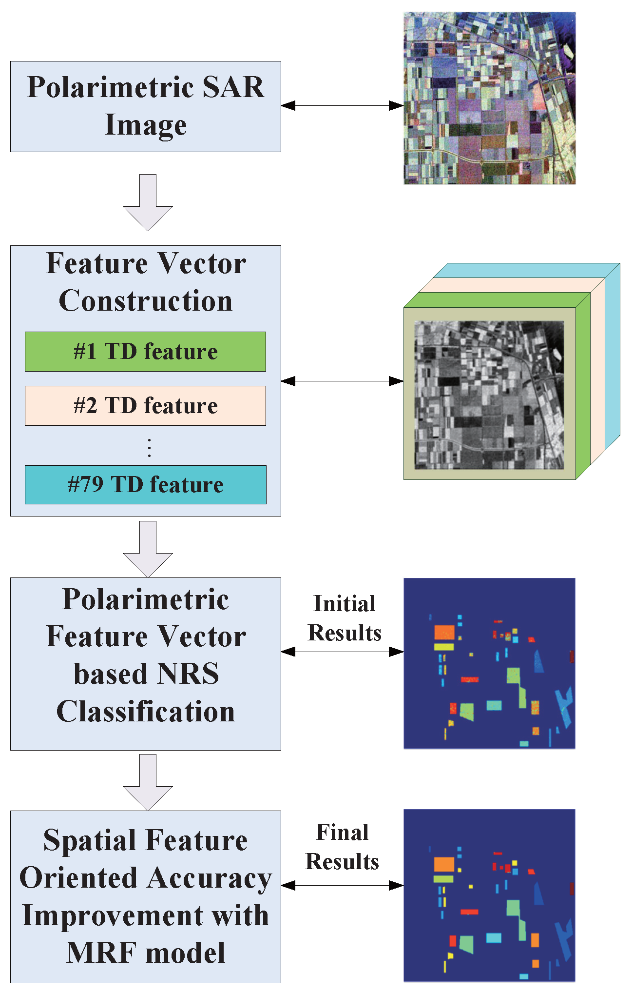
• We construct a comprehensive polarimetric feature vector including 79 TD features. By using the labeled data, the representation-based classifier can exploit the discriminative information within classes contained in the 79-dimensional feature spaces.
• We introduce the NRS classifier considering within-class variations to measure the similarity of the polarimetric feature vector between the test pixel and the labeled pixels and further employ the GC algorithm for spatial information mining.
• We propose a PolSAR imagery-oriented transformation function that connects the residual from NRS and the probability for the MRF model.

The rest of this paper is organized as follows. Section 2 mainly introduces the TD methodology, the NRS classifier and the MRF model. Section 3 specifically describes the proposed NRS-MRF classification framework and gives a detailed introduction for how to effectively combine the NRS classifier with the MRF model for polarimetric SAR images. Then, the experimental results and analysis are presented in Section 4. Finally, conclusions are drawn in Section 5.

2. Methodology

In this section, we will briefly introduce some background knowledge on SAR polarimetric feature extraction and classification. First, several representative polarimetric decomposition features and their intrinsic mechanisms are described and analyzed. The detailed extraction methods are illustrated to show how the raw scattering coefficients are translated into decomposition components. Second, the principle of the nearest-regularized subspace classifier is deduced to demonstrate its efficiency and accuracy with $l_2$-norm regularization. Finally, the MRF model is employed to incorporate the spatial contextual information into the polarimetric classification results.

2.1. Polarimetric Feature Vector Construction

Target decomposition theorems are aimed at providing such an interpretation based on sensible physical constraints such as the average target being invariant to changes in the wave polarization basis [48]. Polarimetric targeted decomposition theory was firstly proposed by Huynen [20] for interpreting the scattering mechanisms of the ground targets, which mainly include surface scattering, dihedral scattering, volume scattering, and so on. Since this original work, there have been many other proposed decompositions that can be classified into four main types [48]:

• Those based on the Kennaugh matrix [K](Huynen [20], Barnes [29] and Yang [27]);
• Those using an eigenvector or eigenvalues analysis of the covariance matrix [C] or coherency matrix [T] (Cloude [49], van Zyl [22], Cloude and Pottier [25], Holm [50] and the multiple-component scattering model (MCSM) [51]);
• Those based on a model-based decomposition of the covariance matrix [C] or the coherency matrix [T] (Freeman [21], Freeman and Durden [52], Yamaguchi [26] and Neumann [23]);
• Those employing coherent decomposition of the scattering matrix [S] (Krogager [24] and Touzi [53]).

Among the four categories of TD algorithms, the former three categories belong to the incoherent decomposition, which is usually used to process the coherent matrix [T], covariance matrix [C] and Kennaugh matrix [K] for representing them as a linear combination. The coherent TD algorithm is used to process the scattering matrix [S] for representing the polarimetric information of the point target and the distributed target. Accordingly, the 12 incoherent TD algorithms and two coherent TD algorithms are employed together to generate 79 features produced by each pixel sample, as shown in

Table 1. The target decomposition features. MCSM, multiple-component scattering model.

Decomposition	Order Numbers	Components
H/$\alpha$/A	1–11	$H{}^{\#}$, $\alpha {}^{\#}$, $A{}^{\#}$, $\lambda {}^{\#}$, $\beta {}^{\#}$, $\gamma {}^{\#}$, $\delta$,
		$(1-H)(1-A){}^{\#}$, $(1-H)A{}^{\#}$, $H(1-A){}^{\#}$, $HA{}^{\#}$
Yang (3 components)	12–14	$f_s$ $f_d{}^{\#}$ $f_v$
Yang (4 components)	15–18	$f_s$ $f_d$ $f_v{}^{\#}$ $f_c$
Barnes (i)	19–21	$T_{11T}$ $T_{22T}{}^{\#}$ $T_{33T}$
Barnes (ii)	22–24	$T_{11T}{}^{\#}$ $T_{22T}$ $T_{33T}$
Cloude	25–27	$T_{11}{}^{\#}$ $T_{22}{}^{\#}$ $T_{33}{}^{\#}$
Freeman	28–29	$P_G{}^{\#}$ $P_V{}^{\#}$
Freeman–Durden	30–32	$P_S{}^{\#}$ $P_D{}^{\#}$ $P_V{}^{\#}$
Holm (1)	33–35	$T_{11}{}^{\#}$ $T_{22}{}^{\#}$ $T_{33}$
Holm (2)	36–38	$T_{11}{}^{\#}$ $T_{22}{}^{\#}$ $T_{33}{}^{\#}$
Huynen	39–41	$T_{11T}{}^{\#}$ $T_{22T}{}^{\#}$ $T_{33T}{}^{\#}$
Krogager	42–44	$k_S$ $k_D{}^{\#}$ $k_H$
MCSM	45–50	$M_S{}^{\#}$ $M_D$ $M_{DH}$ $M_H{}^{\#}$ $M_V{}^{\#}$ $M_W{}^{\#}$
Neuman	51-53	$\left|\delta \right|{}^{\#}$ $\varphi {}^{\#}$ $\tau {}^{\#}$
Tsvm	54-69	$\alpha {}^{\#}$ $\varphi {}^{\#}$ $\psi {}^{\#}$ $\tau {}^{\#}$
Van zyl	70-72	$V_O$ $V_D{}^{\#}$ $V_V$
Yamaguchi (3 components)	73-75	$f_s$ $f_d$ $f_v$
Yamaguchi (4 components)	76-79	$f_s$ $f_d{}^{\#}$ $f_v$ $f_c$
Total	79

Note: The implications of decomposition components can be found in the cited references, which are not stated here in detail. ‘#’ indicates that this TD feature is selected to form the 49 features in the Experimental section.

. The representations of PolSAR imagery and the main TD algorithms will be briefly interpreted in the following part.

2.1.1. PolSAR Data Representations

The information of the PolSAR data is contained in four channels, respectively $HH$, $HV$, $VH$ and $VV$, which indicate four linear orthogonal polarization combinations. Assuming the data are processed with the spatial average under monostatic mode, the complex backscattering matrix [S] for each image pixel at a specific incidence angle can be expressed as:

$$\left[S\right]=\left[\begin{array}{cc}{S}_{hh}& S_{hv}\\ S_{vh}& S_{vv}\end{array}\right]$$

(1)

where the subscript h indicates the horizontal polarization channel and the subscript v represents the vertical polarization channel. Under the monostatic backscattering case, there exists the reciprocity theorem, i.e., $S_{hv}=S_{vh}$. We discuss this backscattering case in the following part of the paper.

From the scattering matrix [S], polarimetric information is usually interpreted by the second-order polarimetric descriptors’ coherent matrix and covariance matrix. The multilook coherent matrix $\left[T\right]$ and covariance matrix $\left[C\right]$ can be expressed as follows.

$$\left[T\right]=〈\overrightarrow{k}·{\overrightarrow{k}}^H〉$$

(2)

$$\left[C\right]=〈\overrightarrow{\Omega }·{\overrightarrow{\Omega }}^H〉$$

(3)

where $〈·〉$ denotes the ensemble average, the superscript H indicates the complex conjugation and transpose of the vector and matrix, $\overrightarrow{k}$ is the Pauli-based scattering vector and $\overrightarrow{\Omega }$ is the lexicographic scattering vector. These two vectors can be specified by vectorizing the scattering matrix [S] and are defined as the following in the backscattering case.

$$\overrightarrow{k}=\frac{1}{\sqrt{2}}{[S_{hh}+S_{vv},S_{hh}-S_{vv},2S_{hv}]}^T$$

(4)

$$\overrightarrow{\Omega }={[S_{hh},\sqrt{2}{S}_{hv},S_{vv}]}^T$$

(5)

where the superscript T indicates the transpose of the vector. Accordingly, the coherency matrix $\left[T\right]$ and covariance matrix $\left[C\right]$ are $3\times 3$ in the monostatic backscattering case.

The Kennaugh matrix containing nine parameters can be expressed as follows:

$$\left[K\right]=\left[\begin{array}{cccc}{A}_0+B_0& C& H& F\\ C& A_0+B& E& G\\ H& E& A_0-B& D\\ F& G& D& -A_0+B_0\end{array}\right]$$

(6)

with

$$\begin{array}{ll}\hfill A_0& =\frac{1}{4}{\left|S_{hh}+S_{vv}\right|}^2\hfill \\ \hfill B_0& =\frac{1}{4}{\left|S_{hh}-S_{vv}\right|}^2+{\left|S_{hv}\right|}^2,B=\frac{1}{4}{\left|S_{hh}-S_{vv}\right|}^2-{\left|S_{hv}\right|}^2,\hfill \\ \hfill C& =\frac{1}{2}{\left|S_{hh}-S_{vv}\right|}^2,D=\mathrm{Im}\left\{S_{hh}{S_{vv}}^{*}\right\}\hfill \\ \hfill E& =\mathrm{Re}\left\{{S_{hv}}^{*}(S_{hh}-S_{vv})\right\},F=\mathrm{Im}\left\{{S_{hv}}^{*}(S_{hh}-S_{vv})\right\}\hfill \\ \hfill G& =\mathrm{Im}\left\{{S_{hv}}^{*}(S_{hh}+S_{vv})\right\},H=\mathrm{Re}\left\{{S_{hv}}^{*}(S_{hh}+S_{vv})\right\}\hfill \end{array}$$

(7)

where the superscript * denotes the complex conjugation; the nine parameters are called the Huynen parameters. These parameters are roll angle dependent corresponding to the target rotation along the radar line-of-sight and contain real physical target information [48]. In the case of a pure target, there exists a one-to-one correspondence between the Kennaugh matrix and the coherency matrix. To sum up, these four matrices [S], [T], [C], [K] are the basis and object of TD algorithms for feature extraction.

2.1.2. Kennaugh Matrix-Based Decompositions

The basis of this kind of TD algorithm is the phenomenological theory proposed by Huynen. The basic idea of the Huynen target decomposition theorem is to separate from the incoming data stream a part that would be identified with a single average target and a residue component. It is argued that this approach follows the perception in the desire to distinguish a required object from its clutter environment. Huynen decomposition can be denoted as follows.

$$\left[T\right]=\left[T_0\right]+\left[T_N\right]$$

(8)

where [$T_0$] indicates the single target component and [$T_N$] indicates the residual component.

Actually, there exist three ways in which the measured coherency $\left[T\right]$ matrix can be factorized into a pure target [$T_0$] and a distributed N-target [$T_N$]. The original decomposition proposed by Huynen is one of the three possible decomposition structures. Those other two decomposition structures are presented later by Barnes and Holm and are also employed in the feature vector.

2.1.3. Eigenvector-Based Decompositions

The residue matrix in the Huynen decomposition is not invariant under the wider class of transformations, as well as the eigenvectors. In order to observe other types of fluctuations of the target vector, more general polarization basis invariant forms of decomposition are developed, which is the decomposition approach based on the eigenvector.

This representative decomposition method is proposed by Cloude and Pottier [25], which relies on the eigenvalue analysis of coherency matrix [T] to generate estimations of the average target scattering matrix parameters.

$$\left[T\right]=\left[U_3\right]\left[\begin{array}{ccc}{\lambda }_1& 0& 0\\ 0& {\lambda }_2& 0\\ 0& 0& {\lambda }_3\end{array}\right]\left[{U_3}^H\right]$$

(9)

with:

$$\left[U_3\right]=\left[{\overline{u}}_1,{\overline{u}}_2,{\overline{u}}_3\right],{\overline{u}}_i=\left[cos{\alpha }_i,sin{\alpha }_{i}cos{\beta }_i{e}^{i{\delta }_i},sin{\alpha }_{i}sin{\beta }_i{e}^{i{\gamma }_i}\right]$$

(10)

where [$U_3$] is a $3\times 3$ complex matrix and ${\lambda }_1>{\lambda }_2>{\lambda }_3\ge 0$ are the corresponding eigenvalues.

In this way, the coherency matrix [T] can be expressed as the sum of three independent targets as follows:

$$\left[T\right]={\lambda }_1\left[T_1\right]+{\lambda }_2\left[T_2\right]+{\lambda }_3\left[T_3\right]$$

(11)

This method rebuilds an average target, and it can be seen as a simple scattering target. Based on the eigenvalue decomposition, many useful parameters can be computed, which include the scattering entropy H, average $\alpha$ angle, anisotropy A and some other intermediate parameters $\lambda$, $\beta$, $\gamma$, $\delta$, as well as parameter combinations (1-H)(1-A), (1-H)A, H(1-A), HA. It should be noted that entropy, scattering angle and anisotropy are important polarimetric features, which can reflect the dominant scattering mechanism, the number of major scattering types and the ratio between them.

Holm provided an alternative physical interpretation of the eigenvalues’ spectrum by interpreting the target as a sum of a single scattering [S] matrix (Rank 1 coherency matrix) plus two noise or remainder terms. This is a hybrid approach, combining an eigenvalue analysis (providing invariance under unitary transformations) with the concept of the single target plus noise model of the Huynen approach. According to different eigenvalue matrix decompositions, Holm decomposition has two representations as follows [48], which are used in the feature vector construction.

$$\left[T\right]=({\lambda }_1-{\lambda }_2)\left[T_1\right]+({\lambda }_2-{\lambda }_3)(\left[T_1\right]+\left[T_2\right])+{\lambda }_3\left[I\right]$$

(12)

or

$$\left[T\right]=({\lambda }_1-{\lambda }_3)\left[T_1\right]+({\lambda }_2-{\lambda }_3)\left[T_2\right]+{\lambda }_3\left[I\right]$$

(13)

where

$$\left[T_1\right]+\left[T_2\right]+\left[T_3\right]=\left[I\right]$$

(14)

2.1.4. Model-Based Decompositions

The model-based decomposition is based on the physical scattering mechanism of the target and decomposes the coherent matrix into surface scattering, dihedral scattering, volume scattering, helix scattering or a partial scattering combination for the specific application scenario.

The Freeman–Durden decomposition method decomposes the target into three parts: a canopy scattering part from a cloud of randomly-oriented dipoles, a double bounce scattering part from a pair of orthogonal surfaces with different dielectric constants and a Bragg scattering part from a moderately rough surface [52]. In the decomposition method, the [T] matrix can be expressed as:

$$\left[T\right]=P_S\left[T_S\right]+P_D\left[T_D\right]+P_V\left[T_V\right]$$

(15)

where $P_S$, $P_D$, $P_V$ correspond to the power of the single bounce scattering part, the double bounce scattering part and the volume scattering part and [$T_S$], [$T_D$], [$T_V$] are the coherency matrices of the three scattering mechanism obtained from scattering models, respectively.

The Yamaguchi decomposition decomposes the target into four scattering mechanisms following the Freeman–Durden decomposition. The decomposition adds a helix scattering power as the fourth component to deal with the non-reflection symmetric scattering cases [26]. Like the Freeman–Durden decomposition, the [T] matrix can be expressed as:

$$\left[T\right]=f_s\left[T_S\right]+f_d\left[T_D\right]+f_v\left[T_V\right]+f_c\left[T_H\right]$$

(16)

where $f_s$, $f_d$, $f_v$ and $f_c$ correspond to the power of the single bounce scattering part, the double bounce scattering part, the volume scattering part and the helix scattering part.

2.1.5. Coherent Decompositions

The objective of the coherent decompositions is to express the measured scattering matrix [S] as a combination of basis matrices corresponding to canonical scattering mechanisms. The coherent target decomposition is useful if only one dominant target component is expected, e.g., dihedral or trihedral edge contributions in urban areas or as calibration targets. Hence, it could be applied to the case of high-resolution, low-entropy scattering problems.

The Krogager decomposition presents a relation to directly measurable quantities and therefore to the actual physical scattering mechanisms represented by the component matrices. In the Krogager decomposition, a symmetric scattering matrix [S] is decomposed into three coherent components that have a physical interpretation in terms of sphere, diplane and helix targets under a change of rotation angle and are defined as follows.

$$\left[S\right]=e^{j\phi }\left\{e^{j{\phi }_S}{k}_S\left[S_s\right]+k_D\left[S_d\right]+k_H\left[S_h\right]\right\}$$

(17)

where $S_s$, $S_d$ and $S_h$ denote the Sinclair matrix of the sphere, diplane and helix; $k_S$, $k_D$, $k_H$ are all real coefficients of those components.

In this research, some other decomposition approaches of these four types are employed to extract polarimetric features, such as Yang decomposition [27], MCSM method [51], Touzi method [53], van Zyl decomposition [22], and so on. The details of each decomposition method can be found in the relevant literature.

2.2. Nearest Regularized Subspace

Assume a given hyperspectral dataset with training samples $\mathbf{X}={\left\{{\mathbf{x}}_i\right\}}_{i=1}^n$ in ${\Re }^d$ and the class label $w_i\in \left\{1,2,\dots ,C\right\}$, where d is the number of spectral variables (bands), C is the number of classes and n is the total number of training samples.

An approximation of the test sample $\mathit{y}$ is represented via a linear combination of available training samples per class. For each class, we can calculate the approximation ${\mathit{y}}_l$ as:

$${\mathit{y}}_l={\mathit{X}}_l·{\mathbf{\alpha }}_l$$

(18)

where ${\mathbf{X}}_l$ is a matrix with the size of $d\times n_l$, $n_l$ is the number of available training samples for class l, ${\displaystyle \sum _{l=1}^C}{n}_l=n$ and ${\mathbf{\alpha }}_l$ represents the weight vector coefficients with the size of $n_l\times 1$ for the linear combination. Suppose we have obtained the weight vector; the label of the test sample is determined by the residual between $\mathit{y}$ and ${\mathit{y}}_l$, which is represented as:

$$r_l\left(\mathit{y}\right)={∥\mathbf{y}-{\mathit{y}}_l∥}_2=∥\mathit{y}-{\mathit{X}}_l·{{\mathbf{\alpha }}_l∥}_2$$

(19)

After that, the class label is then derived according to the class of the most accurate representation (i.e., the minimum value of the residuals for all the classes),

$$class\left(\mathit{y}\right)=arg\underset{l=1,2,\dots ,C}{min}{\mathrm{r}}_l\left(\mathit{y}\right)$$

(20)

In NRS [36], the weight vector for the linear combination is solved as follows,

$${\mathbf{\alpha }}_l=argmin{∥\mathit{y}-{\mathit{X}}_l·{\mathbf{\alpha }}_l∥}_2^2+\lambda ∥{\mathbf{\Gamma }}_{l,\mathit{y}}·{{\mathbf{\alpha }}_l∥}_2^2$$

(21)

The ${\mathbf{\Gamma }}_{l,\mathit{y}}$ is a biasing Tikhonov matrix specific to each class l and test sample y, and the $\lambda$ is a global regularization parameter, which is used to balance the minimization between the residual and regularization terms. For the NRS classifier, we design the diagonal elements of matrix ${\mathbf{\Gamma }}_{l,\mathit{y}}$ in the form of:

$${\mathbf{\Gamma }}_{l,\mathit{y}}=\left[\begin{array}{ccc}∥\mathit{y}-{{\mathit{x}}_{l,1}∥}_2& \cdots & 0\\ ⋮& \ddots & ⋮\\ 0& \cdots & ∥\mathit{y}-{{\mathit{x}}_{l,n_l}∥}_2\end{array}\right]$$

(22)

where ${\mathit{x}}_{l,1},{\mathit{x}}_{l,2},\dots \dots ,{\mathit{x}}_{l,n_l}$ are the columns of ${\mathit{X}}_l$ for the class l. Commonly, Euclidean distance will be used for measuring the similarity between the testing sample and training sample and then to vote for the test sample belonging to the proper label. According to the formulas defined in Equation (21) and Equation (22), the approximation ${\mathit{y}}_l$ of each test sample $\mathit{y}$ can be expressed as:

$${\mathit{y}}_l={\mathit{X}}_l{\left({\mathit{X}}_l^T{\mathit{X}}_l+\lambda {\mathbf{\Gamma }}_{l,y}^T{\mathbf{\Gamma }}_{l,y}\right)}^{-1}{\mathit{X}}_l^T\mathit{y}$$

(23)

We notice that the solution of weight vector has a closed form in NRS. Another similar classifier is CRC [38], whose difference is using an identity matrix Iinstead of the regularization term in Equation (4). In [36], experimental results demonstrated that NRS significantly outperforms CRC for hyperspectral image classification, which turns out to be reasonable. Using a biasing Tikhonov matrix ${\mathbf{\Gamma }}_{l,\mathit{y}}$ to mine the data distribution, the samples in ${\mathit{X}}_l$, which are dissimilar to $\mathit{y}$ in terms of the Euclidean distance, should be given less contribution towards the linear combination than those that are more similar. In NRS, the more relevant weight vector ${\alpha }_l$ makes the approximation ${\mathit{y}}_l$ from the correct class have better similarity with the test sample, which results in much better classification performance than CRC does.

2.3. MRF Model

The pixel-wise NRS classifier has been demonstrated to be effective [36]; however, for the PolSAR classification, the image representation of the same category object is always the block-wise manner, under which the spatial information may have the potential to further improve the classification accuracy.

In the field of machine vision, image analysis is usually defined as the modeling problem. The MRF model [41,42], widely used in image analysis, provides a convenient and consistent modeling approach with context-dependent entities or intrinsically linked with features.

Previous work pointed out the advantages and disadvantages of seeking the joint probability and the conditional probability in the MRF model. From those, GC [44,45,54,55] turns out to be an effective technique, whose energy function can arise from the Bayesian labeling of the first-order MRF model [55]. This algorithm is closely related to the min-cut technique, which is to find the cheapest cut among all cuts separating the terminals.

In the MRF model, we have the probability of the test pixel ${\mathbf{y}}_p$ (note that ${\mathbf{y}}_p$ has the same meaning as the aforementioned $\mathbf{y}$) for each class, and the energy function $\mathrm{E}(·)$ of ${\mathbf{y}}_p$ for class l can be represented as,

$$\mathrm{E}\left({\mathbf{y}}_p\left|w_p=l\right.\right)=\mu {\mathrm{E}}_{data}\left({\mathbf{y}}_p\left|w_p=l\right.\right)+{\mathrm{E}}_{smooth}\left({\mathbf{y}}_p\left|w_p=l\right.\right)$$

(24)

$${\mathrm{E}}_{data}\left({\mathbf{y}}_p\left|w_p=l\right.\right)=\sum _{p\in P}{\mathrm{D}}_p\left({\mathbf{y}}_p\left|w_p=l\right.\right)$$

(25)

where ${\mathrm{D}}_p$ is the spectral energy function for ${\mathbf{y}}_p$ and $\mu$ is the balance parameter. ${\mathrm{E}}_{smooth}\left({\mathbf{y}}_p\left|w_p=l\right.\right)$ means the extent on piecewise smoothness,

$${\mathrm{E}}_{smooth}\left({\mathbf{y}}_p\left|w_p=l\right.\right)=\sum _{q\in N_p}{\mathrm{B}}_{〈p,q〉}\left(1-\delta \left(w_p,w_q\right)\right)$$

(26)

where $w_p$ and $w_q$ are the labels, $\delta$ is the Kronecker delta function ($\delta$($w_p$,$w_q$) = 1 if $w_p$ = $w_q$, and $\delta$($w_p$,$w_q$) = 0 otherwise), ${\mathrm{B}}_{〈p,q〉}$ is viewed as the penalty between ${\mathbf{y}}_p$ and ${\mathbf{y}}_q$ [45], ${\mathbf{y}}_q$ represents the adjacent pixel to ${\mathbf{y}}_p$ and ${\mathbf{N}}_p$ is the set of neighbors for the given pixel ${\mathbf{y}}_p$. Commonly, the more similar these neighboring pixels are, the larger the value will be. If they are totally different, ${\mathrm{B}}_{〈p,q〉}$ will be definitely zero.

3. Proposed Method

In the previous section, the related works have been introduced in detail, including the polarimetric decomposition features, representation-based classifier and MRF model. Next, the overall processing flow from the raw data to classification results will be described to illustrate how the NRS-MRF algorithm measures the pixel similarity in high-dimensional polarimetric decomposition features space.

In general, the proposed method consists of four steps, respectively pre-processing (polarimetric filtering), feature vector construction, NRS classification and classification optimization with spatial information, as shown in Figure 1. As the input of the classification procedure, the fully-polarimetric SAR image is firstly processed with the refined Lee filter to reduce speckle. Next, 18 kinds of polarimetric decomposition operations are performed on each image pixel and turn the polarimetric SAR images into a data cube of a high-dimensional feature space. Then, some labeled samples are randomly selected to construct a structured dictionary, and other samples are taken into account as test samples. After the preparation of classification, the NRS classifier calculates the residual distance and probability belonging to each class consequently. Finally, the optimized labels are calculated according to the probability and local energy function.

3.1. Feature Vector Construction and Similarity Measurement

As for the NRS classification algorithm, a few labeled samples are utilized to form a dictionary, and the testing sample is projected onto the dictionary to get the sparse representation coefficients, which are used to calculate reconstruction errors and finally identify the class label. The sample dimension is just the feature dimension, and the sparse coefficient dimension is related to the size of the dictionary. It can be seen that the precise selection of a low-dimensional feature space is not necessary, and the NRS algorithm can exploit the discriminative information behind the high-dimensional feature space through the sparse representation coefficients. Therefore, we can catenate tens of TD features to construct a high-dimensional feature vector to characterize each pixel sample for further sparse representation processing.

Once the feature vector for each pixel is extracted, the NRS-based similarity measurements are conducted among the test pixels and the structured dictionary. For each test pixel, the residuals to all classes are calculated and can be used for initial classification considering polarimetric features only, as shown in Figure 1.

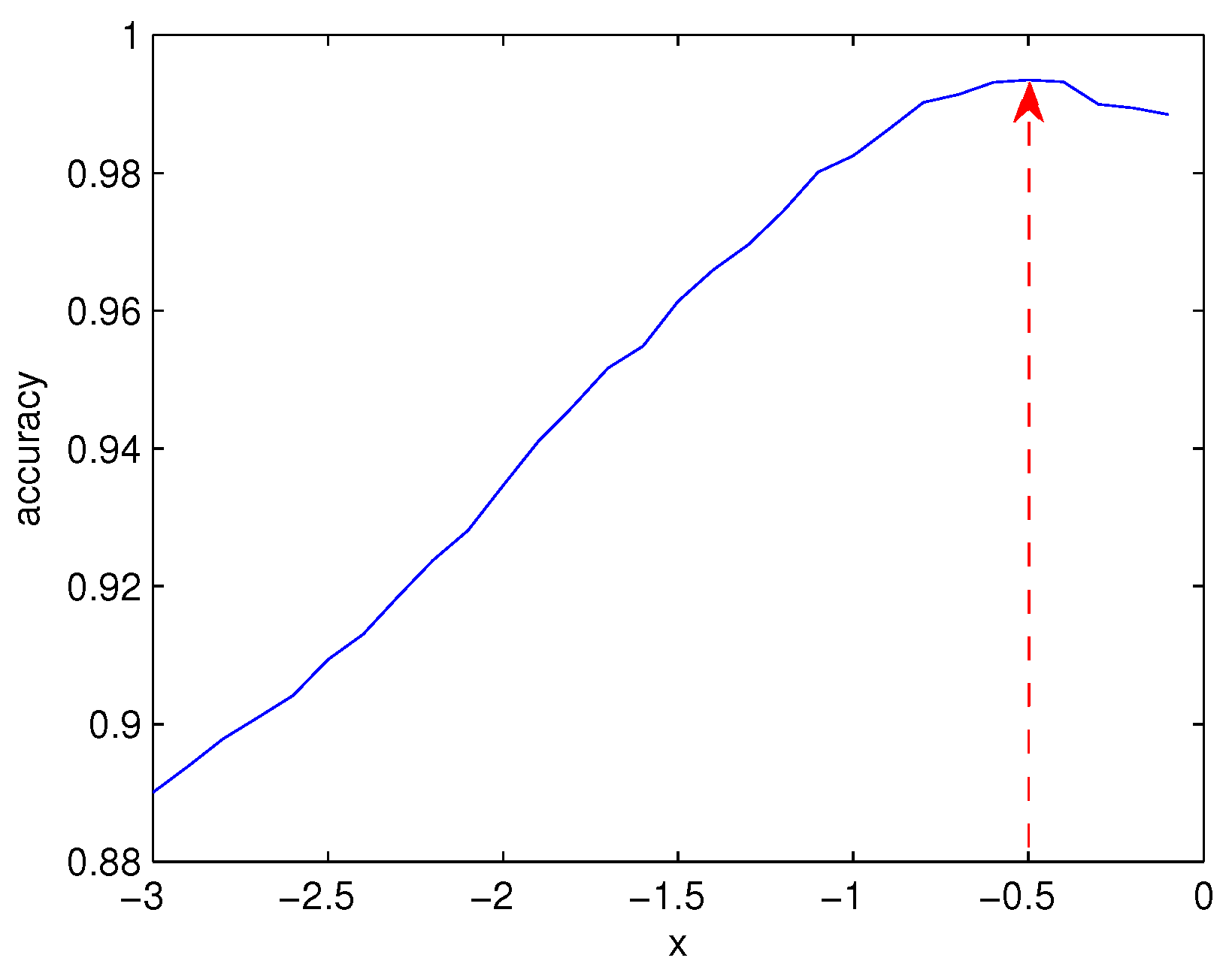
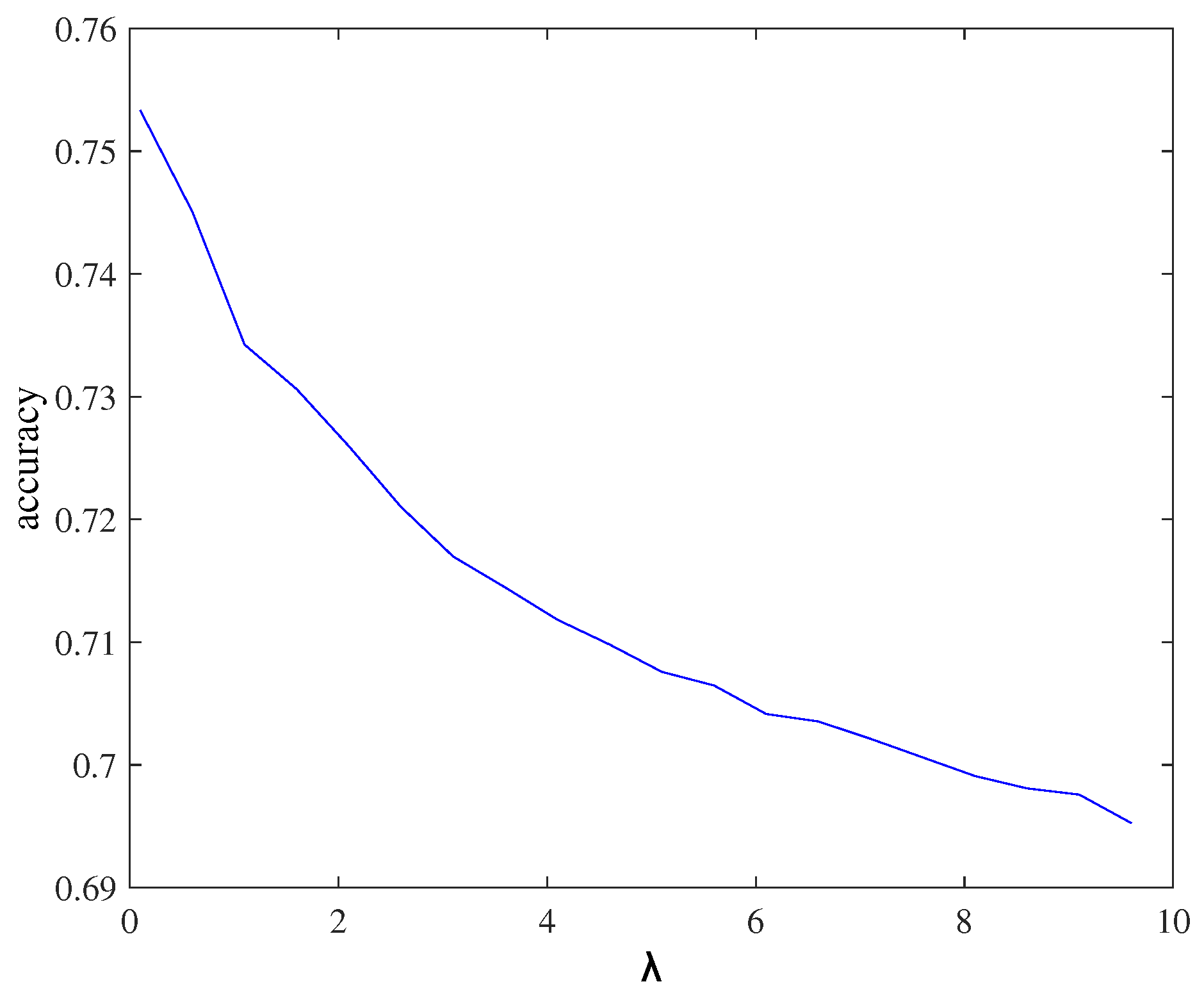
3.2. Parameter Tuning of Transformation Function

In the NRS algorithm, the residual (reconstruction error) for each class is calculated. The smaller the residual of this class, the higher the probability of belonging to this class. As previously mentioned, the GC theory is used to solve the MRF model, which acquires the probability as its input. Therefore, we should attempt to transform the residual for each class to the probability for each class. According to the above analysis, it is reasonable to postulate that the transformation should be a decreasing function of the residual, and the following conditions should be imposed on function f,

$$f\left(0\right)=1,\underset{r_l\to \infty }{lim}f\left(r_l\right)=0$$

(27)

which indicates a decreasing function, and $r_l$ represents the residual of the test pixel for class l and is calculated by Equation (19). To map the residuals into probability for all the classes, a common decreasing function is designed to implement the transformation as the following,

$$f\left(r_l\right)=\frac{{r_l}^x}{{\displaystyle \sum _{l=1}^C}{r_l}^x}$$

(28)

where x is a tuning parameter for PolSAR classification. Note that the range of probability $f\left(r_l\right)$ is from 0–1.

In order to realize the optimal transformation from the residual to probability, we set the range of x to $\left[-3,0\right]$ to investigate the relation between the exponent x and the final classification accuracy. As shown in Figure 2, the optimal value for x is $-0.5$; thus, the transformation function is defined as follows.

$$f\left(r_l\right)=\frac{1/\sqrt{r_l}}{{\displaystyle \sum _{l=1}^C}1/\sqrt{r_l}}$$

(29)

3.3. Feature Vector-Based NRS-MRF Classification

Followed by the above transformation step, for the test pixel $y_p$, we can compute the probability for each class, denoted as $f\left(r_l\right)$. Then, we calculate the energy ${\mathrm{D}}_j\left({\mathbf{y}}_j\left|w_j=l\right.\right)=-ln\left\{f\left(r_l\right)\right\}$ and the energy of this pixel belonging to class l, named as $\mathrm{E}\left({\mathbf{y}}_p\left|w_p=l\right.\right)$. The local energy involves some cut-related algorithms, such as max-flow/min-cut. Finally, we find the label $class\left(\mathbf{y}\right)=arg{min}_{l=1,2,\dots ,C}E\left({\mathbf{y}}_p\left|w_p=l\right.\right)$, which is the optimal classification result derived from combining polarimetric and spatial contextual features, as shown in Algorithm 1.

Algorithm 1 The feature vector-based NRS-MRF classifier.

Input: Fully polarimetric SAR image

Output: Class labels of the entire test image pixels. 1: Preprocessing←polarimetric filtering with refined Lee filter 2: Feature vector construction←stacking 18 categories of polarimetric decomposition features 3: Dictionary construction←feature vector of training data $\mathbf{X}={\left\{x_i\right\}}_{i=1}^n$ with corresponding class label $w_i\in [1,C]$ and feature vector of entire test image with each test sample represented $\mathbf{Y}={\left\{y_p\right\}}_{p=1}^m$. 4: NRS classification: 5: for each $p\in [1,m]$ do 6:   for each $l\in [1,C]$ do 7:     $r\left[p\right]\left[l\right]\leftarrow$ compute the residual distance $r_l\left(y_p\right)$ according to Equation (19); 8:     $f\left(r\left[p\right]\left[l\right]\right)\leftarrow$ compute the optimal probability representation according to Equation (29); 9:   end for 10: end for 11: MRF optimization: 12: for each $p\in [1,m]$ do 13:   $\mathrm{E}\left({\mathbf{y}}_p\left|w_p=l\right.\right)\leftarrow$ compute the local energy according to Equation (24); 14:   $w_p\leftarrow$ compute the final label considering the $argminE$. 15: end for

4. Experimental Results and Analysis

In this section, we design two experiments to discuss the effectiveness of the proposed classification method. Two airborne PolSAR datasets are employed to conduct the experiments for the validation of the proposed classification scheme, which all have ground truth measurements.

4.1. Experiment Data

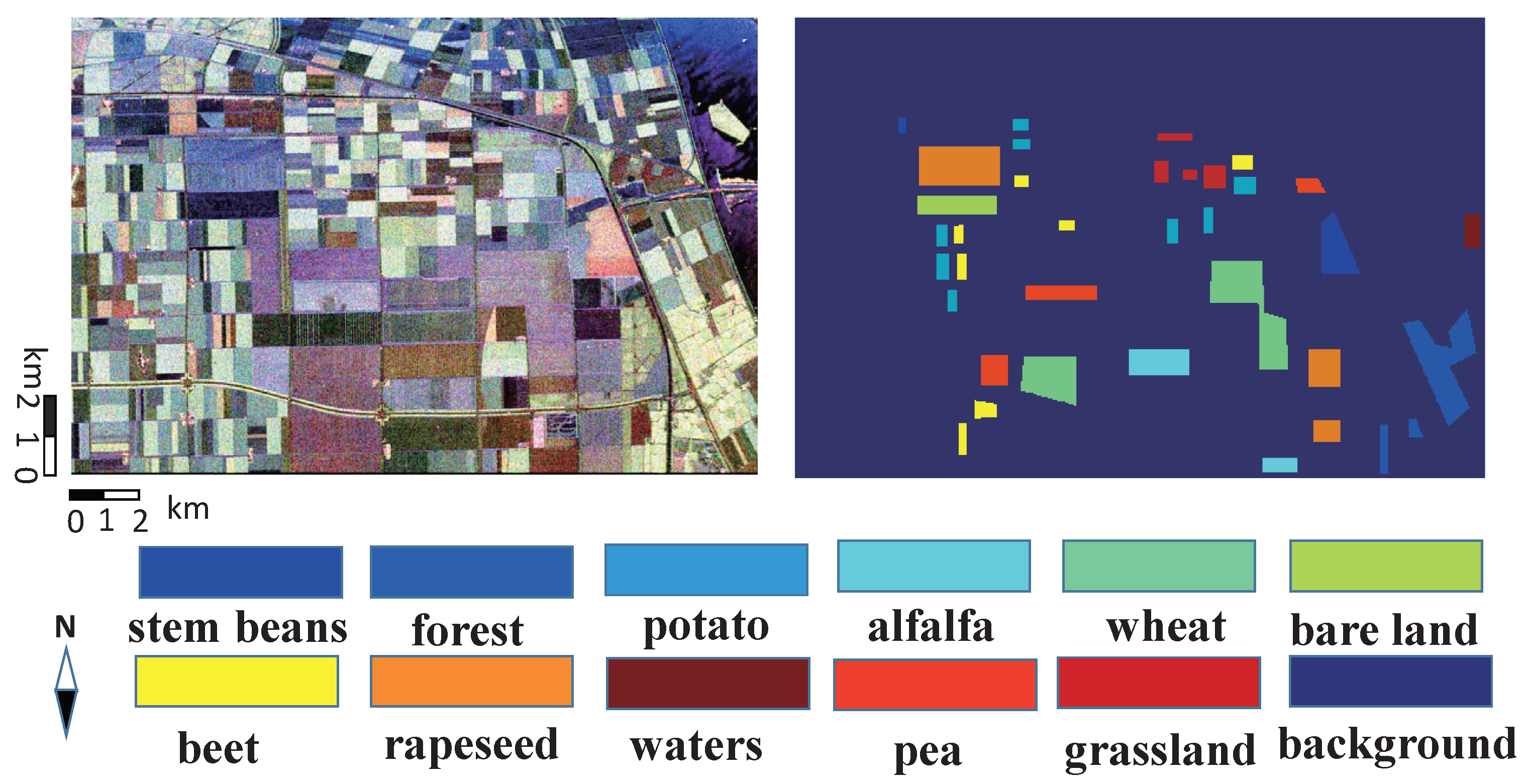
4.1.1. AIRSAR Data in Flevoland I

The first quad-polarimetric SAR dataset is the widely-used L-band data acquired by NASA/JPL AIRSAR system in Flevoland, The Netherlands, August 1989. The incidence angles are around ${20}^{°}$ at the near range and ${44}^{°}$ at the far range. There are 11 different terrain types marked in the ground truth, most of which are agricultural classes, such as stem beans, forest, wheat, bare land, rapeseed, pea, and so on. The size of this datum is $750\times 1024$ pixels. The size of the ground truth data is around 68,188 pixels. The Pauli image and the ground truth image are shown in Figure 3.

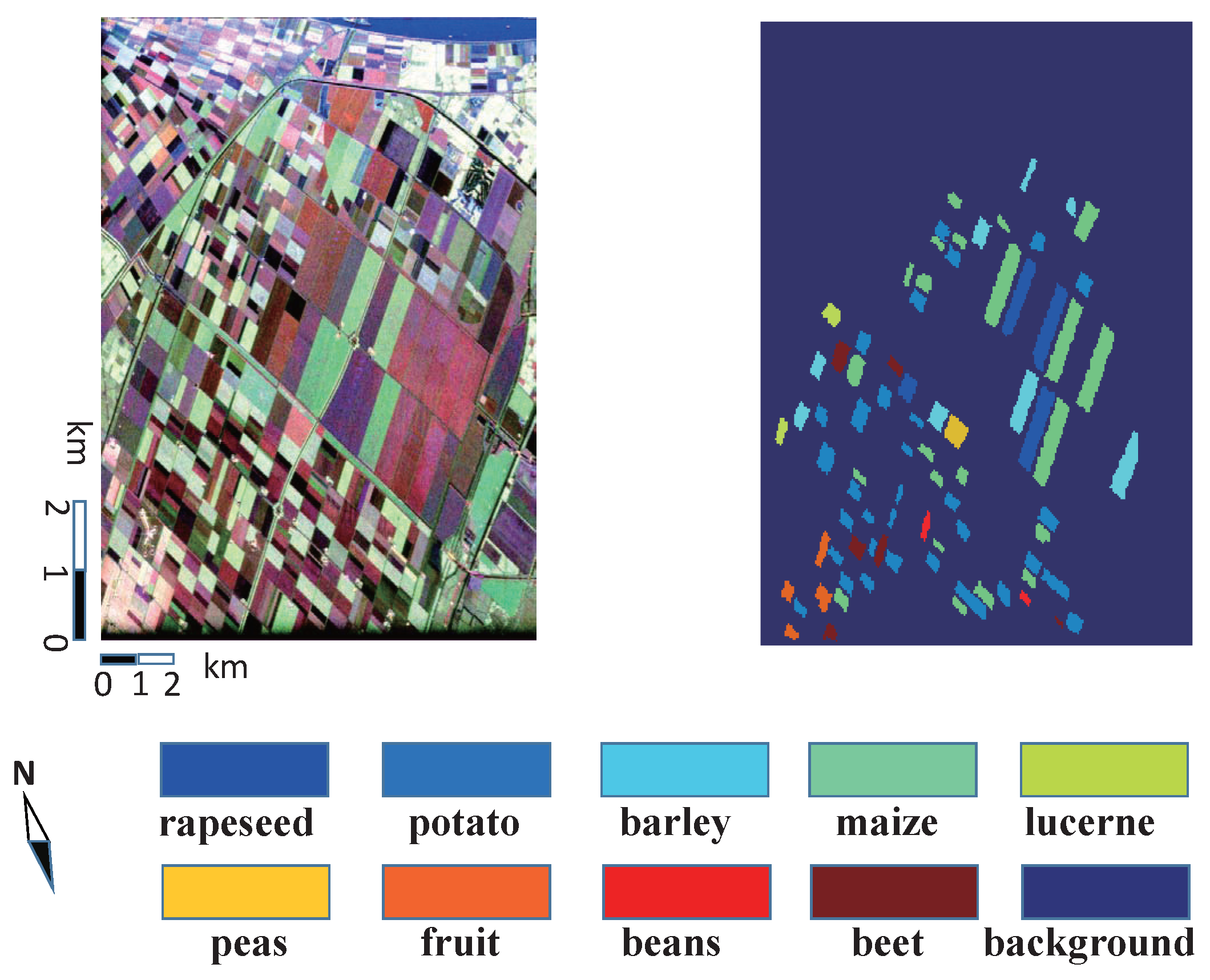
4.1.2. AIRSAR Data in Flevoland II

The second experimental quad-polarimetric SAR dataset is acquired in the same area by the AIRSAR system in June 1991. There are 14 different terrain types measured with the ground truth in the ${30}^{°}$–${60}^{°}$ incidence angle range: potato, beet, maize, wheat, grass, fruit, barley, beans, lucerne, flax, oats, onions, peas and rapeseed. The size of this L-band datum is $1024\times 1279$ pixels. The size of the ground truth data is around 122,928 pixels. The Pauli image and the ground truth image are shown in Figure 4.

4.2. Polarimetric Feature Vector

After the speckle filtering process with the refined Lee method of a $3\times 3$ window size, the polarimetric SAR feature space is constructed by the components of different target decomposition algorithms for each pixel, including those scattering components of Freeman, Huynen, Krogager and Yamaguchi decomposition, as well as the eigenvalues, eigenvectors and their consequential parameters, such as entropy, anisotropy and mean scattering angle. In total, 79 polarimetric features are retrieved from the two datasets, which are listed in Table 1.

On the other side, the processing efficiency will be improved with the decrease of the feature dimension. We design another method of feature vector construction to study the relation between the number of features and the classification accuracy. As a preliminary study, the correlation coefficient is chosen to evaluate the similarity among different features. Firstly, the correlation coefficient between each feature is calculated by the following equation,

$$Coef(X,Y)=\frac{Cov(X,Y)}{\sqrt{Var\left(X\right)Var\left(Y\right)}}$$

(30)

where $Cov(X,Y)$ is the covariance between the single feature vector X and Y and $Var$ is the variance of the feature vector. Secondly, a proper threshold should be set. In the experiment, the empirical threshold of the correlation coefficient is chosen as $97\%$. Thereafter, the features with a correlation coefficient above the threshold are selected as the feature vector. The new feature vector has 49 features, which have been indicated by the ‘#’ sign in Table 1.

4.3. Classifier Parameter Tuning

As a global regularization parameter, the adjustment of $\lambda$ is also important to the NRS algorithm’s performance [37]. By testing different radar data, it is found that basically when $\lambda$ equals a small value, high classification accuracies can be achieved. Therefore, an optimal or suboptimal $\lambda$ should be firstly determined for the subsequent experiments. Due to the need to traverse different values of $\lambda$, the running time will be too long if the entire image takes part in the classification. Therefore, we only select 900 samples as the testing dataset to select the suboptimal value of $\lambda$. Figure 5 displays the trend of classification accuracy as $\lambda$ increases with the Flevoland I data. Thus, $\lambda$ equal to $0.1$ is used for the following experiments.

4.4. Classification Accuracy

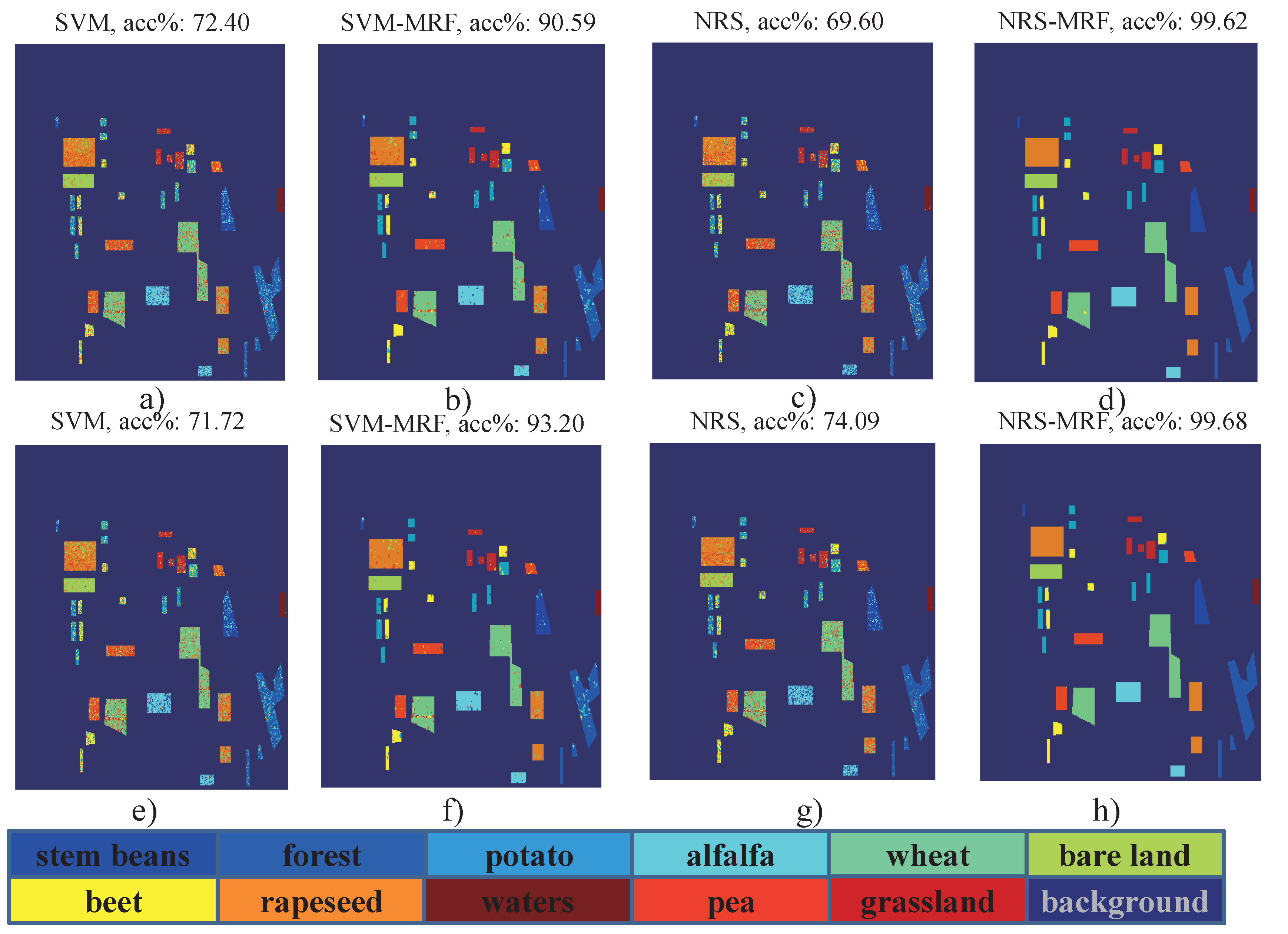
4.4.1. Results and Analysis of Flevoland I Data

NRS is implemented on the AIRSAR dataset in Flevoland I firstly, at the same time comparing with the one combined with MRF, i.e., NRS-MRF, classic SVM and the combination of SVM-MRF. It should also be noted that we will randomly select 300 pixels of each class as the training samples, and the rest of the pixels of each class as the testing samples. This is because for some datasets, there are big differences in the number of pixels between classes, and this imbalance problem could cause bad classification performance.

The classification results with 49 and 79 features are shown in Figure 6a–d and Figure 6e,f, respectively. The reduced feature vector impacts the NRS algorithm by $5\%$ and has little effect on NRS-MRF method. In this sense, MRF not only utilizes the spatial information to improve the accuracy, but also can improve the efficiency through the insensitivity to the feature number. As for the experiments with 79 features, the NRS algorithm can achieve the overall accuracy of $74.09\%$. It is seen that there are many errors existing inside each class area. This phenomenon could be largely reduced when introducing the MRF method, taking the spatial information into consideration. Figure 6h shows the result of NRS-MRF, which is obviously improved with the overall accuracy of $99.68\%$. Most part of the misclassification errors inside the each class disappear. For comparison, the classification results of SVM and SVM-MRF are also shown in Figure 6e,f. The corresponding accuracies are $71.72\%$ and $93.20\%$, respectively.

In order to analyze the classification performance for each class, the confusion matrices of the SVM, NRS, SVM-MRF and NRS-MRF approaches are shown in

Table 2. Confusion matrix for Flevoland I data using SVM.

Class	1	2	3	4	5	6	7	8	9	10	11	Accuracy (%)
1	3189	116	83	725	1	-	3	-	1	3	-	77.38
2	408	7157	1410	817	81	-	163	1	9	63	-	70.8
3	74	557	3169	104	30	-	818	2	43	51	-	65.37
4	783	287	122	3763	30	-	39	1	-	104	3	73.32
5	1	59	87	41	11,592	6	345	789	1002	608	57	79.47
6	-	-	-	-	6	3208	4	202	19	-	12	92.96
7	5	66	940	21	41	-	2343	15	279	267	-	58.91
8	-	9	10	-	1055	1171	153	7622	2324	94	31	61.13
9	-	19	27	-	359	12	344	1144	3146	281	5	58.95
10	1	24	26	65	56	-	146	19	98	2503	-	85.19
11	-	-	-	-	2	-	-	1	-	-	1216	99.75
Total												71.72

,

Table 3. Confusion matrix for Flevoland I data using NRS.

Class	1	2	3	4	5	6	7	8	9	10	11	Accuracy (%)
1	3324	220	33	534	-	-	8	-	-	2	-	80.66
2	249	8802	710	251	14	-	32	2	4	45	-	87.07
3	20	1023	3029	31	12	-	689	-	22	22	-	62.48
4	878	698	59	3366	17	-	17	1	-	96	-	65.59
5	1	99	287	62	11,328	2	287	772	1192	557	-	77.66
6	-	-	-	-	23	2848	-	554	14	-	12	82.53
7	-	87	929	2	20	-	2553	8	164	214	-	64.19
8	-	8	32	1	1114	283	131	8246	2533	120	1	66.13
9	-	16	59	-	457	-	304	975	3230	296	-	60.52
10	5	50	28	38	48	-	104	24	50	2591	-	88.19
11	-	-	2	-	2	5	-	5	-	-	1205	98.85
Total												74.09

,

Table 4. Confusion matrix for Flevoland I data using SVM-MRF.

Class	1	2	3	4	5	6	7	8	9	10	11	Accuracy(%)
1	3900	13	24	183	-	-	-	-	-	1	-	94.64
2	121	9101	354	453	20	-	42	-	1	17	-	90.03
3	3	113	4552	16	14	-	132	1	12	5	-	93.89
4	123	84	28	4831	22	-	9	-	-	35	-	94.13
5	-	14	18	15	13,899	-	130	57	176	278	-	95.28
6	-	-	-	-	-	3386	-	65	-	-	-	98.12
7	-	15	257	-	1	-	3601	-	22	81	-	90.55
8	-	9	-	-	350	332	18	11,283	446	31	-	90.49
9	-	20	6	-	27	-	77	149	4928	130	-	92.34
10	-	13	-	-	1	-	48	-	20	2856	-	97.21
11	-	-	-	-	-	-	-	-	-	-	1219	100
Total												93.21

and

Table 5. Confusion matrix for Flevoland I data using NRS-MRF.

Class	1	2	3	4	5	6	7	8	9	10	11	Accuracy (%)
1	4120	1	-	-	-	-	-	-	-	-	-	99.98
2	-	10,109	-	-	-	-	-	-	-	-	-	100
3	-	-	4848	-	-	-	-	-	-	-	-	100
4	-	-	-	5132	-	-	-	-	-	-	-	100
5	-	-	8	-	14,579	-	-	-	-	-	-	99.95
6	-	-	-	-	-	3451	-	-	-	-	-	100
7	-	-	162	-	-	-	3815	-	-	-	-	95.93
8	-	-	-	-	26	-	-	12,443	-	-	-	99.79
9	-	-	1	-	23	-	-	-	5313	-	-	99.55
10	-	-	-	-	-	-	-	-	-	2938	-	100
11	-	-	-	-	-	-	-	-	-	-	1219	100
Total												99.68

. As for the former three methods, except Class 11, each class has some points wrongly classified, while referring to the NRS-MRF method in Table 5, there are only a few pixels of Classes 7, 8, 9 and 10 classified into the wrong classes. These pixels existed in the margin area of classes, which could probably be affected by the filtering process.

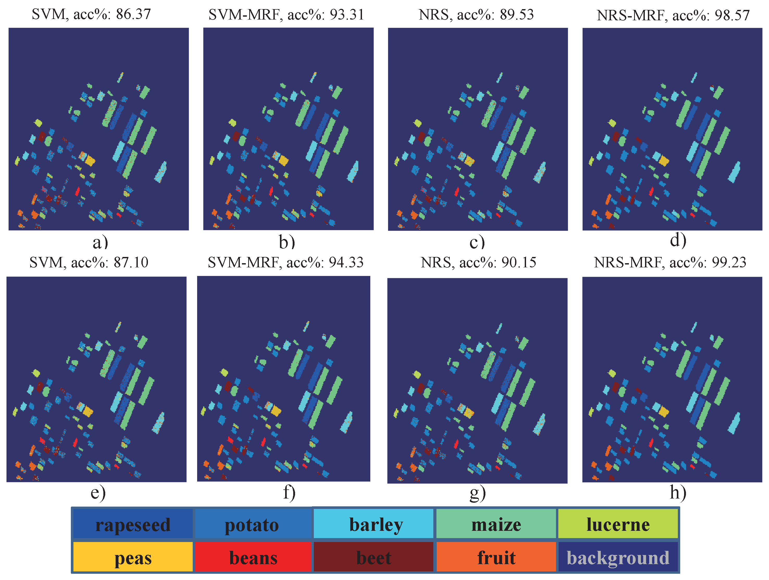
4.4.2. Results and Analysis on Flevoland II Data

Then, the NRS and NRS-MRF are implemented on the AIRSAR dataset in Flevoland II, in comparison with classic SVM, and the combination of SVM-MRF. During the NRS implementation, the regularization parameter $\lambda$ and the x parameter in the conversion equation take the values of 0.6 and $-0.5$, respectively.

The classification results are displayed in Figure 7a–h. For these experimental data, the difference between 49 and 79 features is greatly decreased. Referring to NRS with 79 features, the overall accuracy is $90.15\%$. Similarly, there are many errors existing inside each class area. After applying the combined NRS-MRF method, taking the spatial information into consideration, the classification accuracy is increased to $99.23\%$; while, the classification results of SVM and SVM-MRF are $87.10\%$ and $94.33\%$, respectively. Hence, for this dataset, NRS and SVM are improved by the same scale with the introduction of the MRF method.

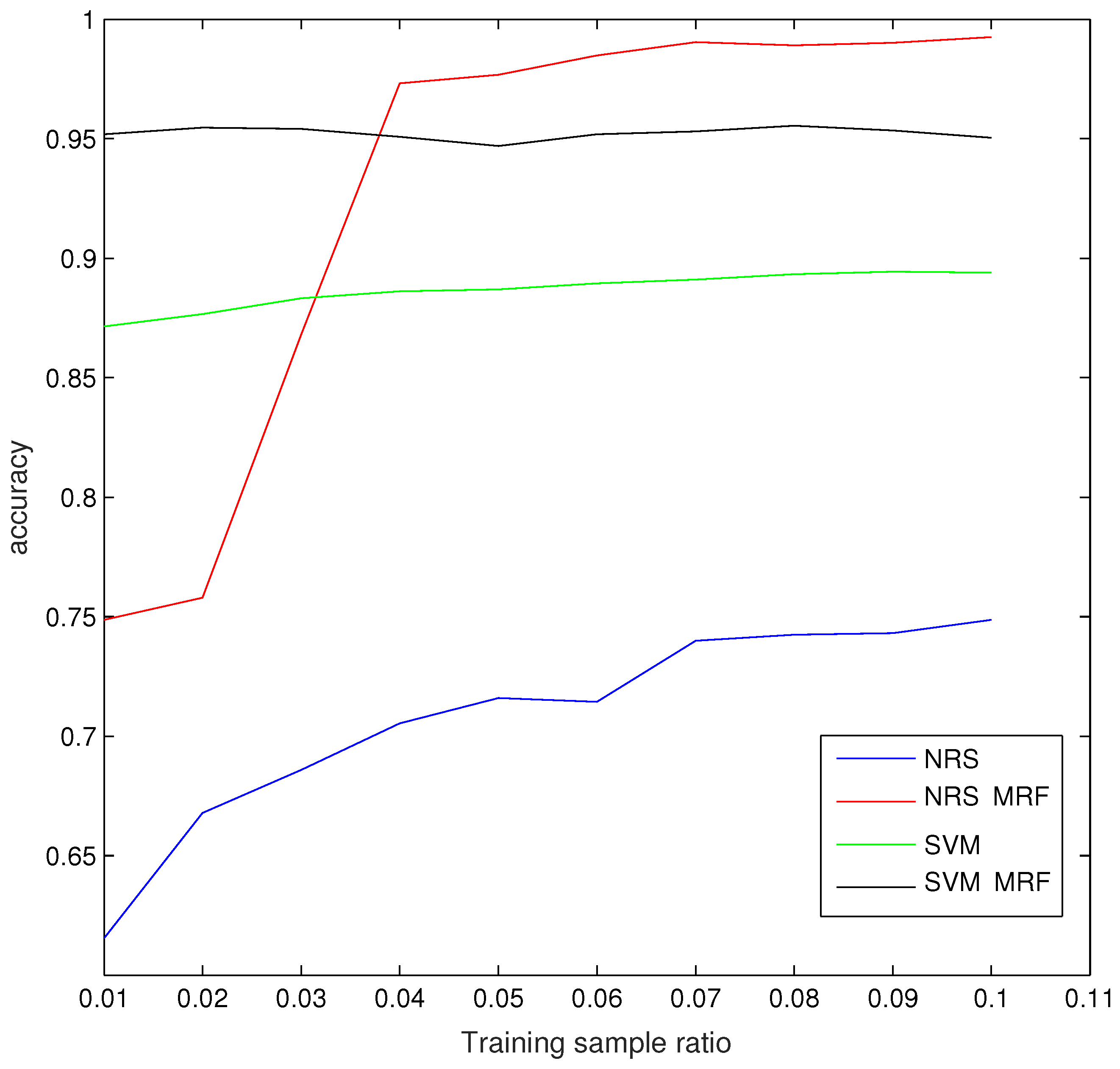
4.5. The Influence of Training Size

After the analysis of the parameter impacts and classification accuracy, it is necessary to discuss the proper rate of samples for training in the whole dataset. Taking the Flevoland I data as an example, we train with different ratios for all four algorithms, not fixed number of 300 training samples; the change tendency is described in Figure 8. It is clear that for all algorithms, $5\%$ is enough to get stable classification accuracy. However, NRS has a big improvement and the best accuracy when combining with MRF, as the rate of training samples increases.

The difference between Figure 8 and Figure 6 may have been noticed. As we mentioned before, Figure 6 is the result when the same amount of samples in each class is used for training, while Figure 8 is from the viewpoint of the same rate of samples in each class for training.

4.6. The Analysis of Classification Performance

As previously mentioned, the proposed method is capable of keeping a good classification performance with the limited training data and the reduced polarimetric features. The main reason may come from the collaboration of NRS and MRF. MRF can greatly decrease the misclassifications based on the good homogeneousness assumption. However, for different sensors and areas, this advantage may be invalid. Therefore, the improvement of MRF or other post-processing methods will be still worth studying in the future research work.

5. Conclusions and Future Work

In this paper, the NRS classifier is employed for polarimetric features extracted from PolSAR images, by the use of TD. Considering that the spatial information is not well utilized, MRF is also introduced to our scheme, since it could provide a basis for modeling contextual constraints. The polarimetric SAR feature space is constructed by the components of different target decomposition algorithms for each pixel, using two airborne PolSAR datasets in Flevoland area. In the implementation of the classification, the impact of the regularization parameter of NRS and the conversion coefficient of MRF on the overall accuracy of classification are analyzed, respectively. Furthermore, the proper number of training samples is also discussed. Experimental results of Flevoland I data demonstrated that the classification accuracy of the proposed NRS-MRF is superior to the original NRS and SVM with $25\%$ and $28\%$, respectively. Moreover, NRS-MRF is even superior to the state-of-the-art SVM-MRF with $6\%$ under the condition of randomly selecting 300 pixels of each class as the training samples. To reach a high classification accuracy, the selected training data ratio should be at least $4\%$. The future work of our group may focus on the study of deep learning, which is used to extract features and classify targets.

References

1. Moreira, A.; Prats-iraola, P.; Younis, M.; Krieger, G.; Hajnsek, I.; Papathanassiou, K. A Tutorial on synthetic aperture radar. IEEE Geosci. Remote Sens. Mag. 2013, 1, 6–43. [Google Scholar] [CrossRef] [Green Version]
2. Lee, J.; Grunes, M.; Ainsworth, T.; Du, L.; Schuler, D.; Cloude, S. Unsupervised classification using polarimetric decomposition and the complex Wishart classifier. IEEE Trans. Geosci. Remote Sens. 1999, 37, 2249–2258. [Google Scholar]
3. Lee, J.; Grunes, M.; Pottier, E. Quantitative comparison of classification capability: Fully polarimetric versus dual and single-polarization SAR. IEEE Trans. Geosci. Remote Sens. 2001, 39, 2343–2351. [Google Scholar]
4. Oh, Y.; Sarabandi, K.; Ulaby, F.T. An empirical model and an inversion technique for radar scattering from bare soil surfaces. IEEE Trans. Geosci. Remote Sens. 1992, 30, 370–381. [Google Scholar] [CrossRef]
5. Dubois, P.C.; Van Zyl, J.; Engman, T. Measuring soil moisture with imaging radars. IEEE Trans. Geosci. Remote Sens. 1995, 33, 915–926. [Google Scholar] [CrossRef]
6. Hajnsek, I. Inversion of Surface Parameters from Polarimetric SAR Data. Ph.D. Thesis, Friedrich Schiller University of Jena (FSU), Jena, Germany, 2001. [Google Scholar]
7. Yin, Q.; Hong, W.; Li, Y.; Lin, Y. Soil moisture change detection model for slightly rough surface based on interferometric phase. J. Appl. Remote Sens. 2015, 9, 095981. [Google Scholar] [CrossRef]
8. Li, Y.; Hong, W.; Pottier, E. Topography retrieval from single-pass POLSAR data based on the polarization-dependent intensity ratio. IEEE Trans. Geosci. Remote Sens. 2015, 53, 3160–3177. [Google Scholar]
9. Gao, G.; Shi, G. CFAR Ship Detection in Nonhomogeneous Sea Clutter Using Polarimetric SAR Data Based on the Notch Filter. IEEE Trans. Geosci. Remote Sens. 2017, 55, 4811–4824. [Google Scholar] [CrossRef]
10. Wei, J.; Li, P.; Yang, J.; Zhang, J.; Lang, F. A New Automatic Ship Detection Method Using L-Band Polarimetric SAR Imagery. IEEE J. Sel. Top. Appl. Earth Obs. Remote Sens. 2017, 7, 1383–1393. [Google Scholar]
11. Masjedi, A.; Zoej, M.; Maghsoudi, Y. Classification of polarimetric SAR images based on modeling contextual information and using texture features. IEEE Trans. Geosci. Remote Sens. 2016, 54, 932–943. [Google Scholar] [CrossRef]
12. Xiang, D.; Ban, Y.; Su, Y. Model-based decomposition with cross scattering for polarimetric SAR urban areas. IEEE Geosci. Remote Sens. Lett. 2015, 12, 2496–2500. [Google Scholar] [CrossRef]
13. Cao, F.; Hong, W.; Wu, Y.; Pottier, E. An Unsupervised Segmentation with an Adaptive Number of Clusters Using the SPAN/H/α/A Space and the Complex Wishart Clustering for Fully Polarimetric SAR Data Analysis. IEEE Trans. Geosci. Remote Sens. 2007, 45, 3454–3467. [Google Scholar] [CrossRef]
14. Fukuda, S.; Hirosawa, H. Support vector machine classification of land cover: Application to polarimetric SAR data. In Proceedings of the 2001 IEEE International Geoscience and Remote Sensing Symposium (IGARSS’01), Sydney, Australia, 9–13 July 2001; Volume 1, pp. 187–189. [Google Scholar]
15. Qi, Z.; Yeh, A.; Li, X.; Lin, Z. A novel algorithm for land use and land cover classification using RADARSAT-2 polarimetric SAR data. Remote Sens. Environ. 2012, 118, 21–39. [Google Scholar] [CrossRef]
16. Liu, H.; Zhu, D.; Yang, S.; Hou, B.; Gou, S.; Xiong, T.; Jiao, L. Semisupervised Feature Extraction with Neighborhood Constraints for Polarimetric SAR Classification. IEEE J. Sel. Top. Appl. Earth Obs. Remote Sens. 2016, 9, 3001–3015. [Google Scholar] [CrossRef]
17. Buono, A.; Nunziata, F.; Migliaccio, M.; Yang, X.; Li, X. Classification of the Yellow River delta area using fully polarimetric SAR measurements. Int. J. Remote Sens. 2017, 38, 6714–6734. [Google Scholar] [CrossRef]
18. Lee, J.; Grunes, M.; Grandi, G.D. Polarimetric SAR speckle filtering and its implication for classification. IEEE Trans. Geosci. Remote Sens. 1999, 37, 2363–2373. [Google Scholar]
19. Foucher, S.; Lopez-Martinez, C. Analysis, evaluation, and comparison of polarimetric SAR speckle filtering techniques. IEEE Trans. Image Process. 2014, 23, 1751–1764. [Google Scholar] [CrossRef] [PubMed]
20. Huynen, J.R. Phenomenological Theory of Radar Targets. Ph.D. Thesis, Technical University, Delft, The Netherlands, 1970. [Google Scholar]
21. Freeman, A. Fitting a two-component scattering model to polarimetric SAR data from forests. IEEE Trans. Geosci. Remote Sens. 2007, 45, 2583–2592. [Google Scholar] [CrossRef]
22. Freeman, A.; van Zyl, J.J.; Klein, J.D.; Zebker, H.A.; Shen, Y. Calibration of Stokes and scattering matrix format polarimetric SAR data. IEEE Trans. Geosci. Remote Sens. 1992, 30, 531–539. [Google Scholar] [CrossRef]
23. Neumann, M.; Ferro-Famil, L.; Pottier, E. A general model-based polarimetric decomposition scheme for vegetated areas. In Proceedings of the International Workshop Science Applications SAR Polarimetry Polarimetric Inferometry (POLINSAR), Frascati, Italy, 26–30 January 2009. [Google Scholar]
24. Krogager, E. New decomposition of the radar target scattering matrix. Electron. Lett. 1990, 26, 1525–1527. [Google Scholar] [CrossRef]
25. Cloude, S.R.; Pottier, E. An entropy based classification scheme for land applications of polarimetric SAR. IEEE Trans. Geosci. Remote Sens. 1997, 35, 68–78. [Google Scholar] [CrossRef]
26. Yamaguchi, Y.; Yajima, Y.; Yamada, H. A four-component decomposition of POLSAR images based on the coherency matrix. IEEE Geosci. Remote Sens. Lett. 2006, 3, 292–296. [Google Scholar] [CrossRef]
27. Yang, J.; Peng, Y.N.; Yamaguchi, Y.; Yamada, H. On Huynen’s decomposition of a Kennaugh matrix. IEEE Geosci. Remote Sens. Lett. 2006, 3, 369–372. [Google Scholar] [CrossRef]
28. Cloude, S.R.; Pottier, E. A review of target decomposition theorems in radar polarimetry. IEEE Trans. Geosci. Remote Sens. 1996, 34, 498–518. [Google Scholar] [CrossRef]
29. Barnes, R.M. Roll-invariant decompositions for the polarization covariance matrix. In Proceedings of the Polarimetry Technology Workshop, Redstone Arsenal, AL, USA, 16–18 Agust 1988; pp. 1–15. [Google Scholar]
30. Shi, L.; Zhang, L.; Yang, J.; Zhang, L.; Li, P. Supervised graph embedding for polarimetric SAR image classification. IEEE Geosci. Remote Sens. Lett. 2013, 10, 216–220. [Google Scholar] [CrossRef]
31. Feng, J.; Cao, Z.; Pi, Y. Polarimetric contextual classification of PolSAR images using sparse representation and superpixels. Remote Sens. 2014, 6, 7158–7181. [Google Scholar] [CrossRef]
32. Zhang, L.; Sun, L.; Zou, B.; Moon, W. Fully polarimetric SAR image classification via sparse representation and polarimetric features. IEEE J. Sel. Top. Appl. Earth Obs. Remote Sens. 2015, 8, 3923–3932. [Google Scholar] [CrossRef]
33. Hou, B.; Ren, B.; Ju, G.; Li, H.; Jiao, L.; Zhao, J. SAR image classification via hierarchical sparse representation and multisize patch features. IEEE Geosci. Remote Sens. Lett. 2016, 13, 33–37. [Google Scholar] [CrossRef]
34. Gou, S.; Li, X.; Yang, X. Coastal zone classification with fully polarimetric SAR imagery. IEEE Geosci. Remote Sens. Lett. 2016, 13, 1616–1620. [Google Scholar] [CrossRef]
35. Pajares, G.; Lopez-Martinez, C.; Sanchez-Liado, F.; Molina, I. Improving Wishart classification of polarimetric SAR data using the Hopfield Neural Network optimization approach. Remote Sens. 2012, 4, 3571–3595. [Google Scholar] [CrossRef] [Green Version]
36. Li, W.; Tramel, E.W.; Prasad, S. Nearest regularized subspace for hyperspectral classification. IEEE Trans. Geosci. Remote Sens. 2014, 52, 477–489. [Google Scholar] [CrossRef]
37. Li, W.; Du, Q.; Xiong, M. Kernel Collaborative Representation With Tikhonov Regularization for Hyperspectral Image Classification. IEEE Geosci. Remote Sens. Lett. 2015, 12, 48–52. [Google Scholar]
38. Zhang, L.; Yang, M.; Feng, X. Sparse representation or collaborative representation: Which helps face recognition? In Proceedings of the IEEE International Conference on Computer Vision (ICCV), Barcelona, Spain, 6–13 November 2011; pp. 471–478. [Google Scholar]
39. Geng, J.; Fan, J.; Wang, H.; Fu, A.; Hu, Y. Joint collaborative representation for polarimetric SAR image classification. In Proceedings of the IEEE International Geoscience and Remote Sensing Symposium (IGARSS), Beijing, China, 10–15 July 2016; pp. 3066–3069. [Google Scholar]
40. Fukuda, S.; Hirosawa, H. A wavelet-based texture feature set applied to classification of multifrequency polarimetric SAR images. IEEE Trans. Geosci. Remote Sens. 1999, 37, 2282–2286. [Google Scholar] [CrossRef]
41. Schick, A.; Bauml, M.; Stiefelhagen, R. Improving Foreground Segmentations with Probabilistic Superpixel Markov Random Fields. In Proceedings of the IEEE Conference on Computer Vision and Pattern Recognition (CVPR), Providence, RI, USA, 16–21 June 2012; pp. 27–31. [Google Scholar]
42. Ghamisi, P.; Benediktsson, J.A.; Ulfarsson, M.O. Spectral-spatial classification of hyperspectral images based on hidden Markov random fields. IEEE Trans. Geosci. Remote Sens. 2014, 52, 2565–2574. [Google Scholar] [CrossRef]
43. Borges, J.S.; Bioucas-Dias, J.M.; Marcal, A.R. Bayesian hyperspectral image segmentation with discriminative class learning. IEEE Trans. Geosci. Remote Sens. 2011, 49, 2151–2164. [Google Scholar] [CrossRef]
44. Boykov, Y.; Veksler, O.; Zabih, R. Fast approximate energy minimization via graph cuts. IEEE Trans. Pattern Anal. Mach. Intell. 2001, 23, 1222–1239. [Google Scholar] [CrossRef]
45. Boykov, Y.Y.; Jolly, M.P. Interactive graph cuts for optimal boundary and region segmentation of objects in ND images. In Proceedings of the IEEE International Conference on Computer Vision (ICCV), Vancouver, BC, Canada, 7–14 July 2001; pp. 105–112. [Google Scholar]
46. Li, W.; Prasad, S.; Fowler, J. Hyperspectral image classification using Gaussian mixture models and Markov random fields. IEEE Geosci. Remote Sens. Lett. 2015, 11, 153–157. [Google Scholar] [CrossRef]
47. Wu, Y.; Ji, K.; Yu, W.; Su, Y. Region-based classification of polarimetric SAR images using Wishart MRF. IEEE Geosci. Remote Sens. Lett. 2008, 5, 668–672. [Google Scholar] [CrossRef]
48. Lee, J.S.; Pottier, E. Polarimetric Radar Imaging: From Basics to Applications; CRC Press: Boca Raton, FL, USA, 2009. [Google Scholar]
49. Cloude, S.R. Target decomposition theorems in radar scattering. Electron. Lett. 1985, 21, 22–24. [Google Scholar] [CrossRef]
50. Holm, W.A.; Barnes, R.M. On radar polarization mixed target state decomposition techniques. In Proceedings of the IEEE National Radar Conference, Ann Arbor, MI, USA, 20–21 April 1988; pp. 249–254. [Google Scholar]
51. Zou, B.; Lu, D.; Zhang, L.; Moon, W.M. Eigen-decomposition-based four-component decomposition for PolSAR data. IEEE J. Sel. Top. Appl. Earth Obs. Remote Sens. 2016, 9, 1286–1296. [Google Scholar] [CrossRef]
52. Freeman, A.; Durden, S.L. A three-component scattering model for polarimetric SAR data. IEEE Trans. Geosci. Remote Sens. 1998, 36, 963–973. [Google Scholar] [CrossRef]
53. Touzi, R. Target scattering decomposition of one-look and multi-look SAR data using a new coherent scattering model: The TSVM. In Proceedings of the 2004 IEEE International Geoscience and Remote Sensing Symposium (IGARSS’04), Anchorage, AK, USA, 20–24 September 2004; Volume 4, pp. 2491–2494. [Google Scholar]
54. Khokher, M.R.; Ghafoor, A.; Siddiqui, A.M. Image segmentation using multilevel graph cuts and graph development using fuzzy rule-based system. IET Image Process. 2013, 7, 201–211. [Google Scholar] [CrossRef]
55. Kolmogorov, V.; Zabin, R. What energy functions can be minimized via graph cuts? IEEE Trans. Pattern Anal. Mach. Intell. 2004, 26, 147–159. [Google Scholar] [CrossRef] [PubMed]
Figure 1. Diagram of the proposed method.
Remotesensing 09 01114 g001
Figure 2. Impact of parameter x on the classification accuracy.
Remotesensing 09 01114 g002
Figure 3. Flevoland I dataset: Pauli image (left) and ground truth image (right).
Remotesensing 09 01114 g003
Figure 4. Flevoland II dataset: Pauli image (left) and ground truth image (right).
Remotesensing 09 01114 g004
Figure 5. The influence of the regularization parameter on the classification accuracy for the Flevoland I data.
Remotesensing 09 01114 g005
Figure 6. The classification results for Flevoland I data: (ad) classification with 49 features; (eh) classification with 79 features.
Remotesensing 09 01114 g006
Figure 7. The classification results for Flevoland II data: (ad) classification with 49 features; (eh) classification with 79 features.
Remotesensing 09 01114 g007
Figure 8. The influence of the training sample ratio on classification accuracy for Flevoland I data.
Remotesensing 09 01114 g008