Semi-Automatic System for Land Cover Change Detection Using Bi-Temporal Remote Sensing Images


Abstract
:
1. Introduction
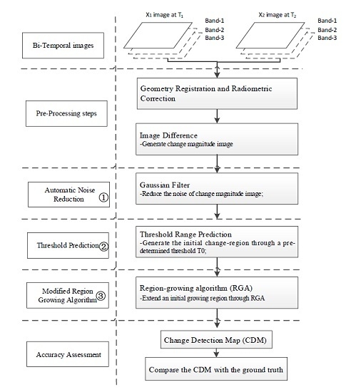
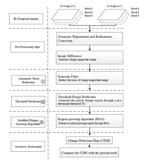
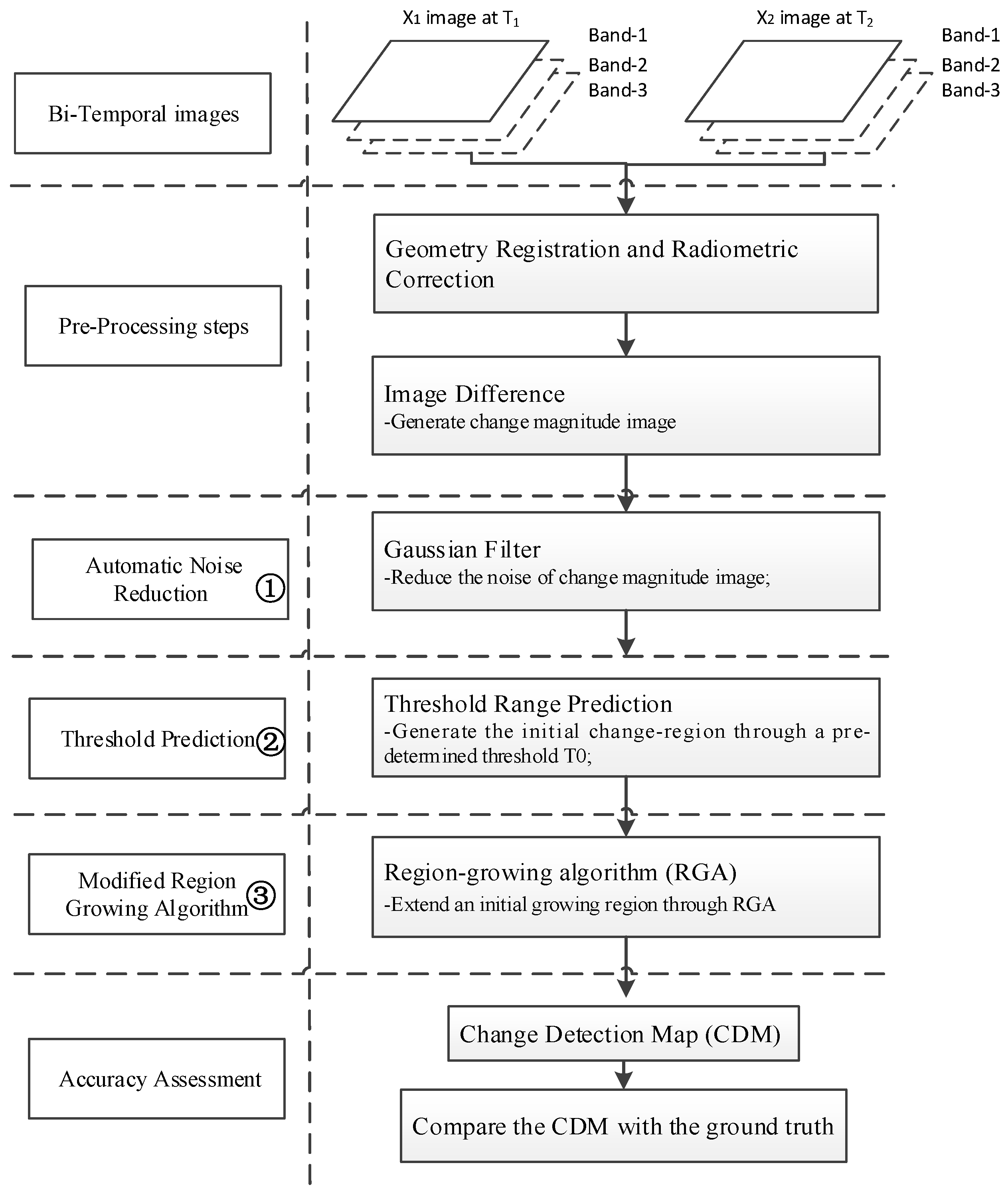
2. Method
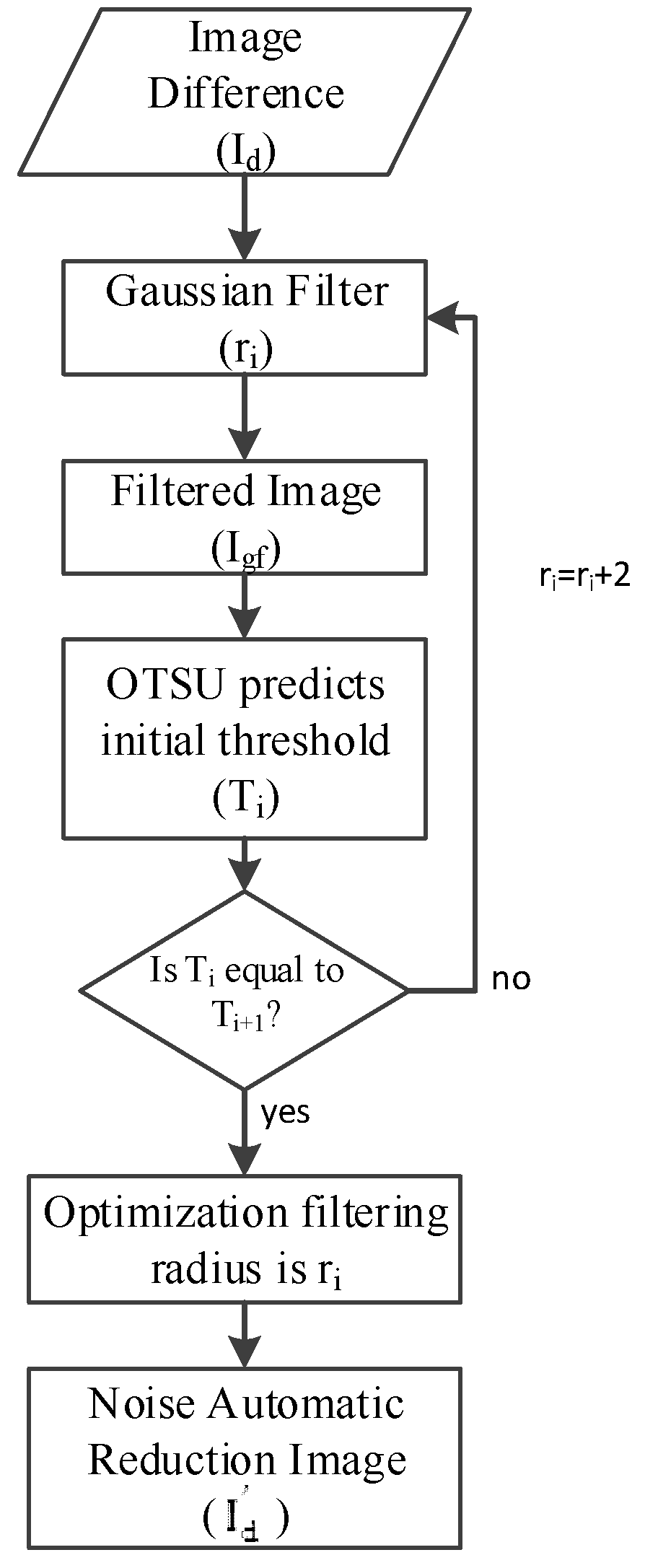
2.1. Automatic Noise Reduction Based on GF
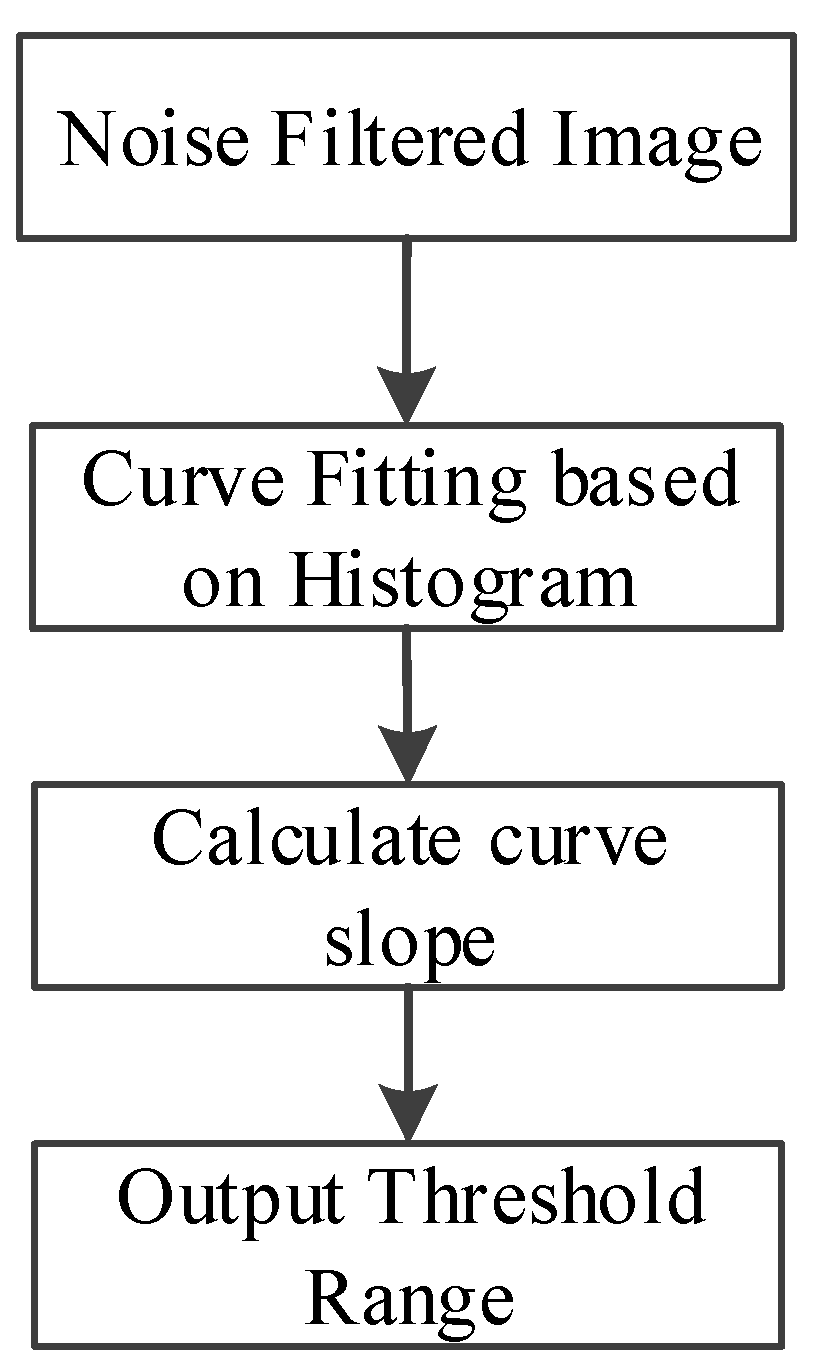
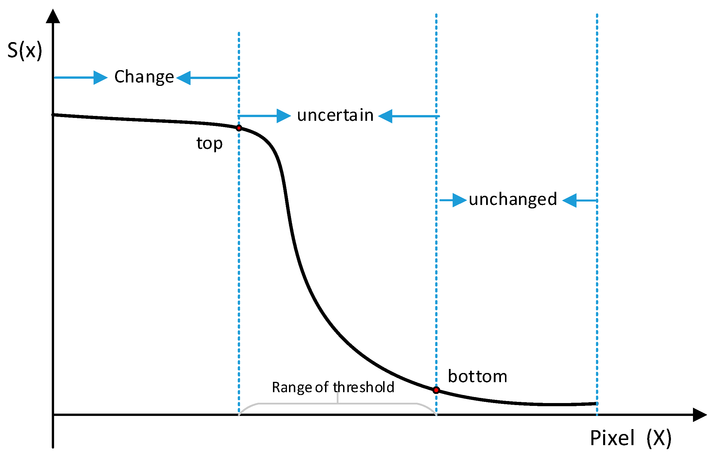
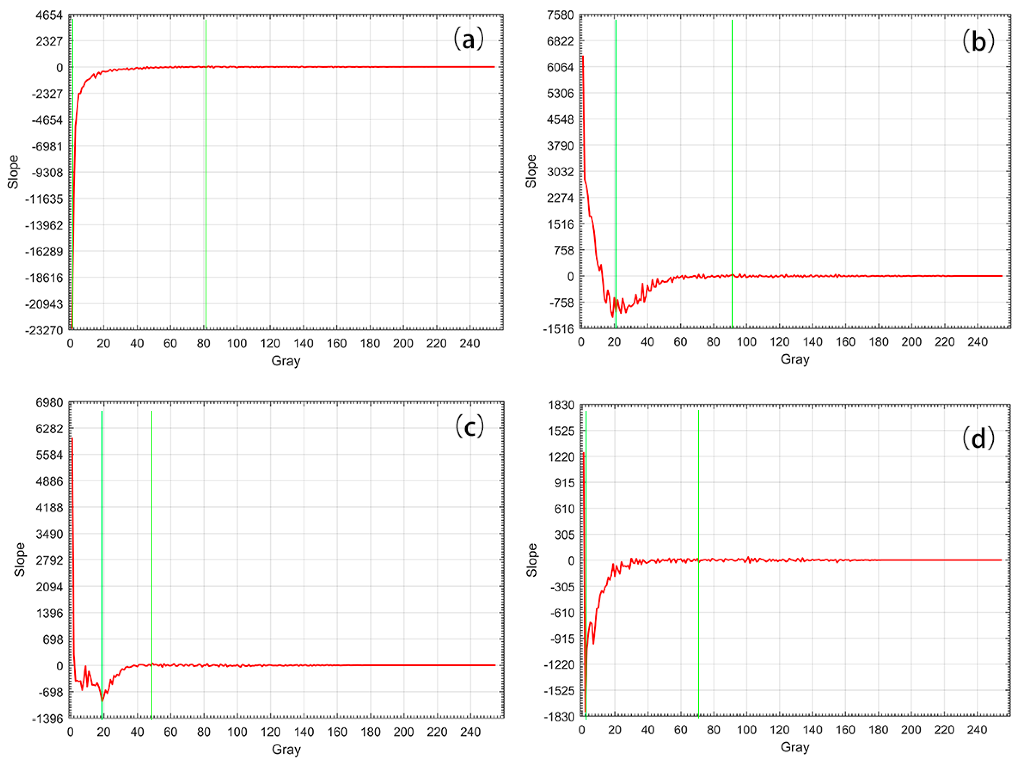
2.2. Threshold Range Prediction (TRP) for Generating the Initial Change Detection Region
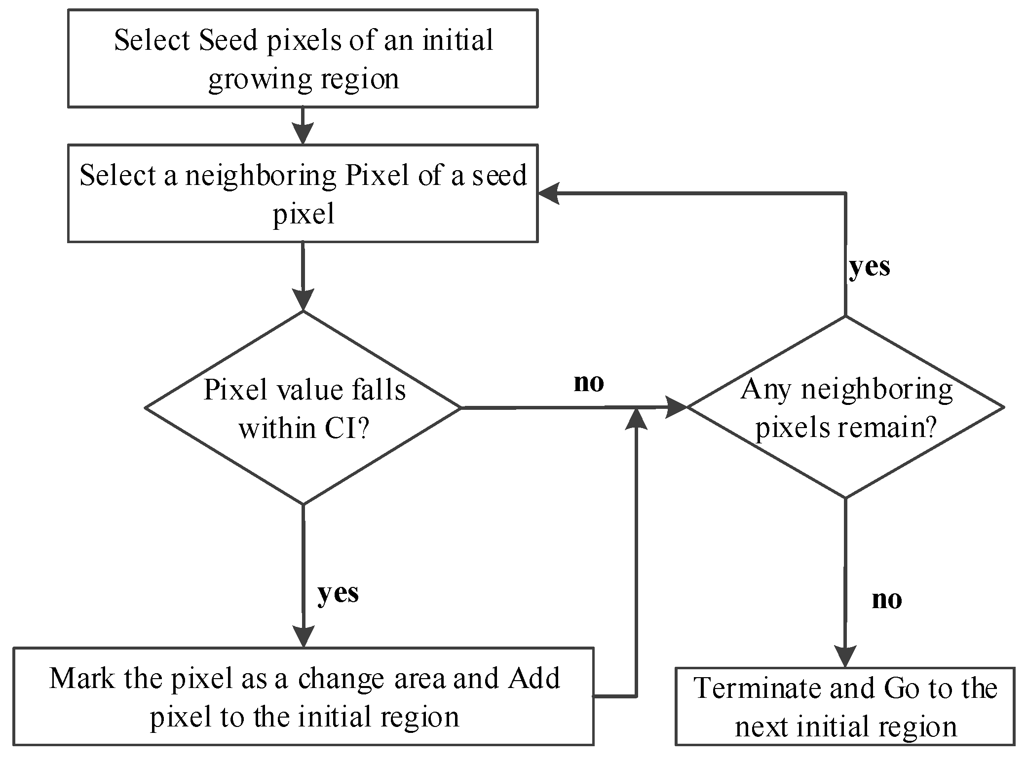
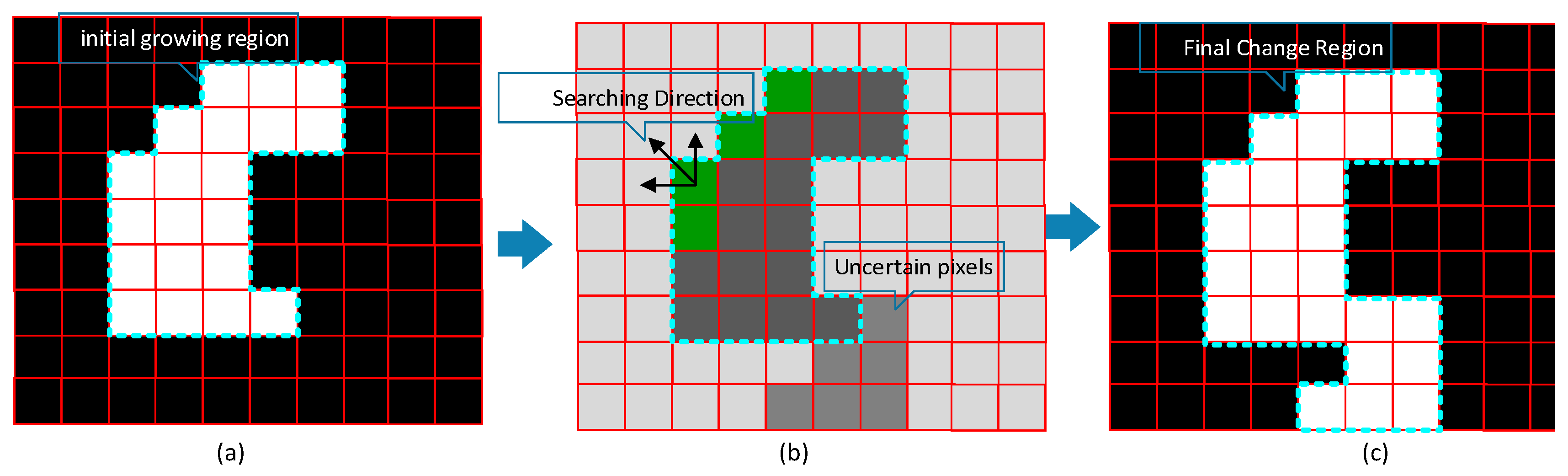
2.3. Modified RGA for Land Cover Change Detection (LCCD)
3. Experiment
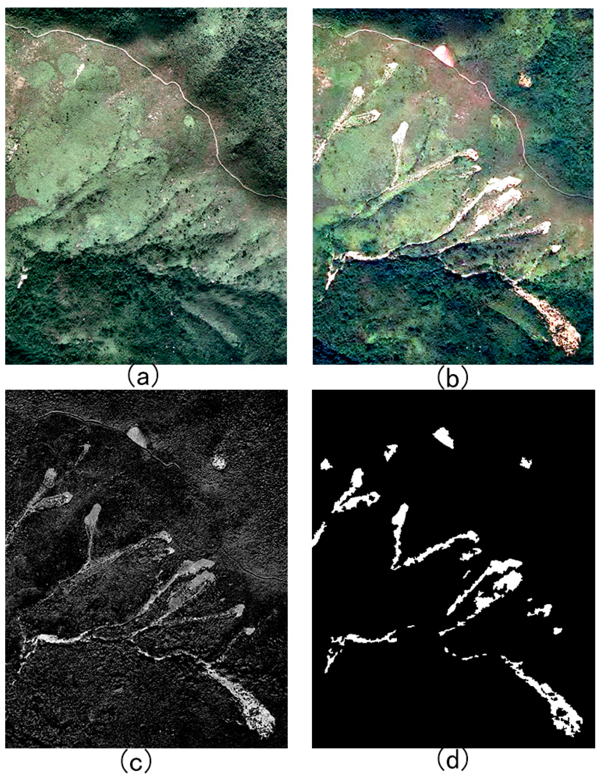
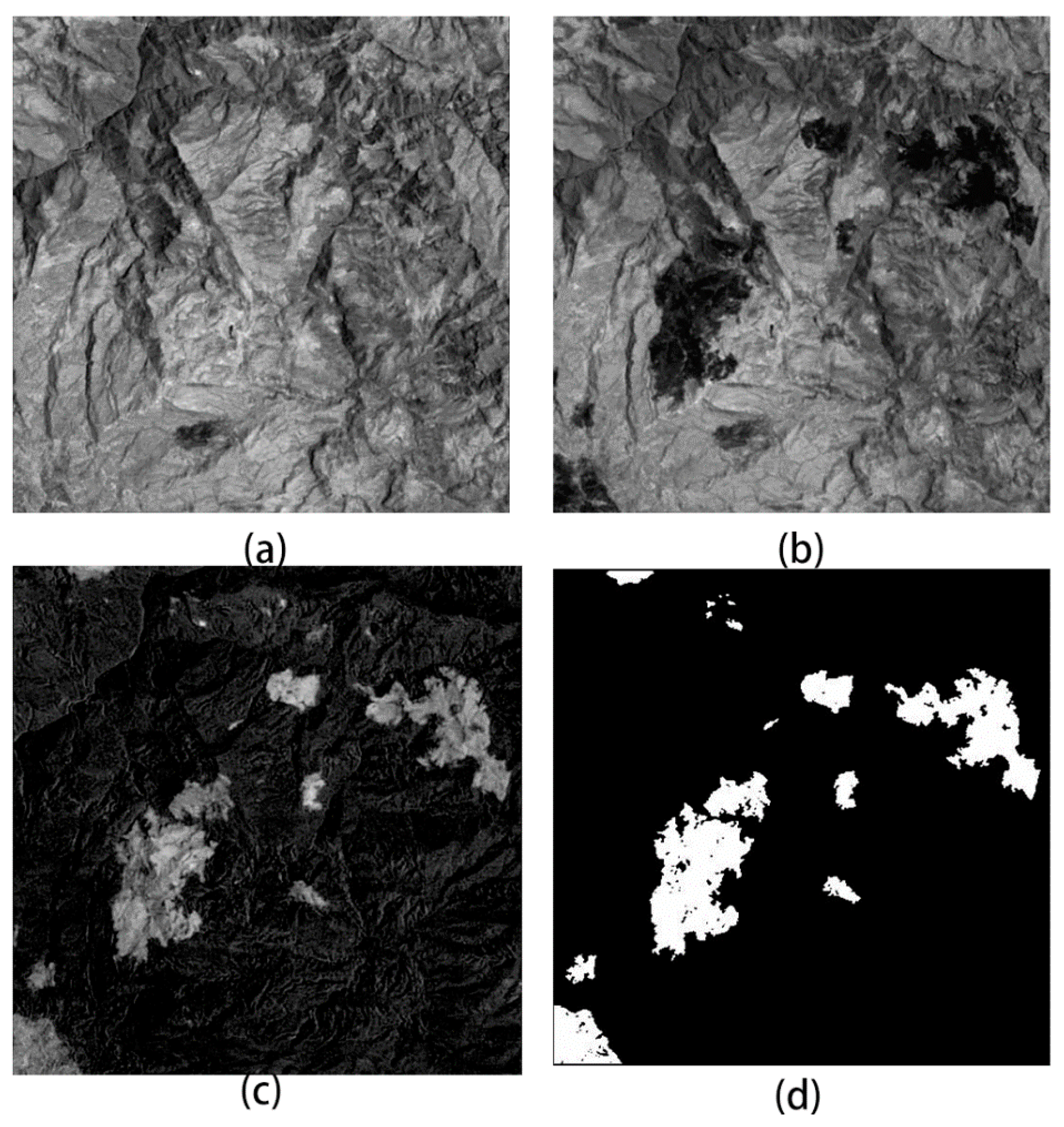
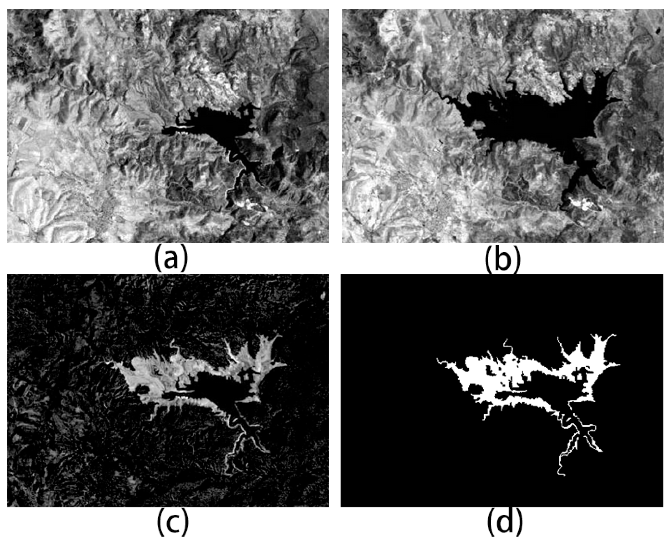
3.1. Dataset Description
3.2. Experimental Setup and Parameter Setting
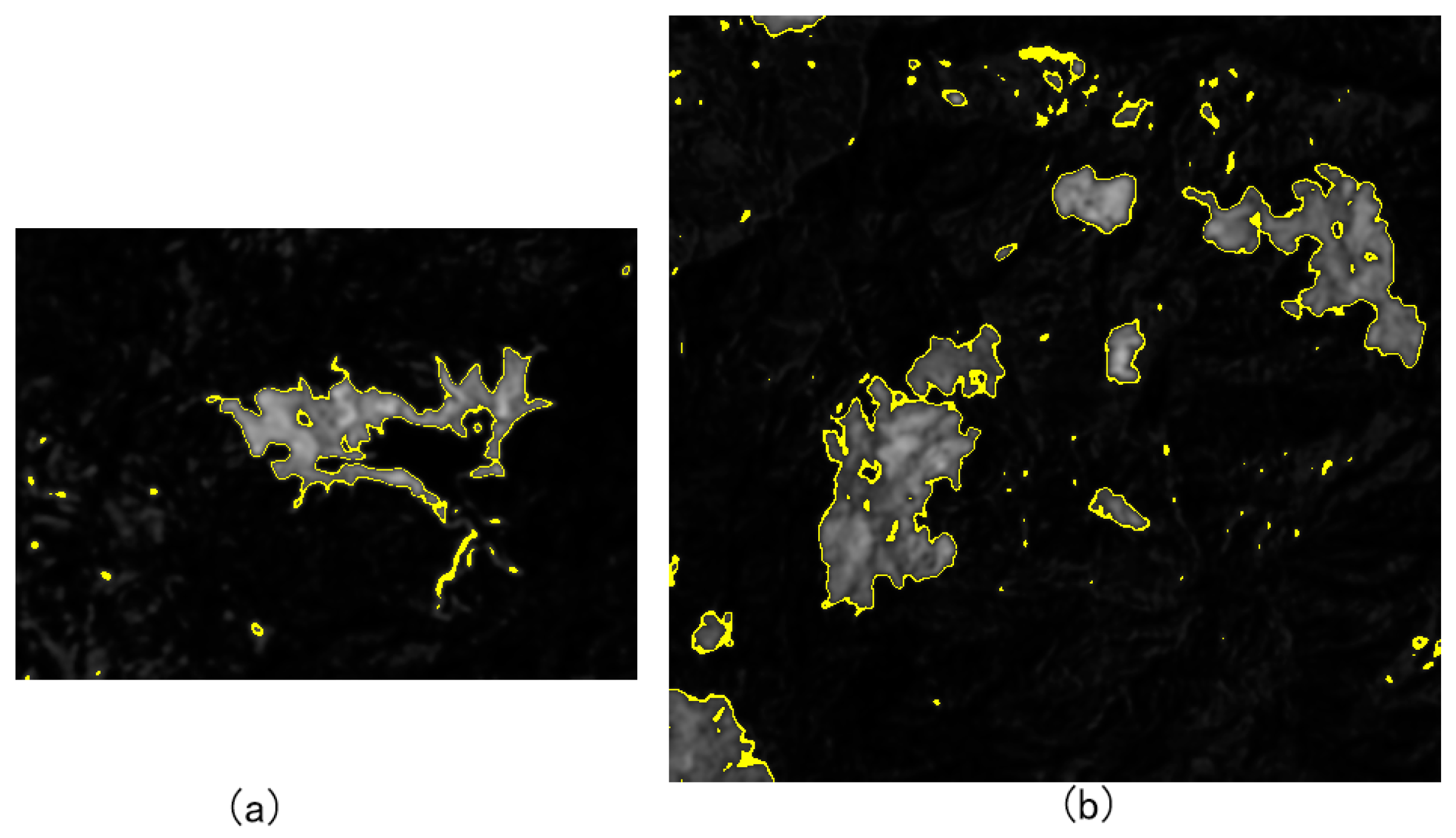
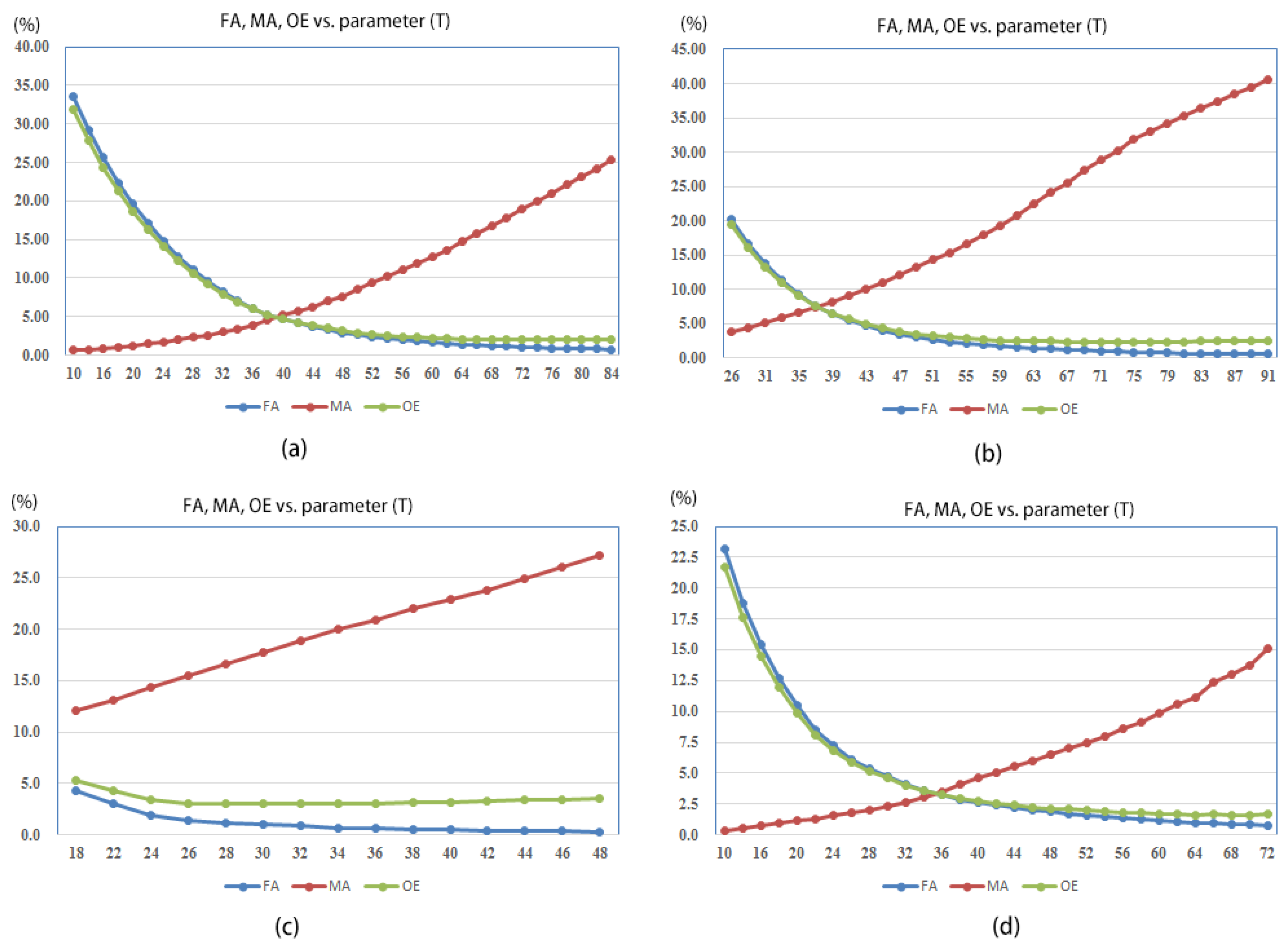
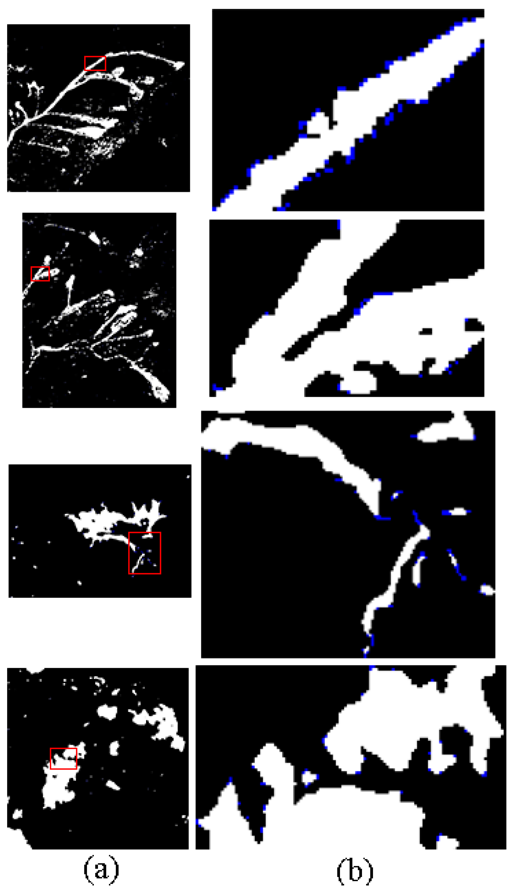
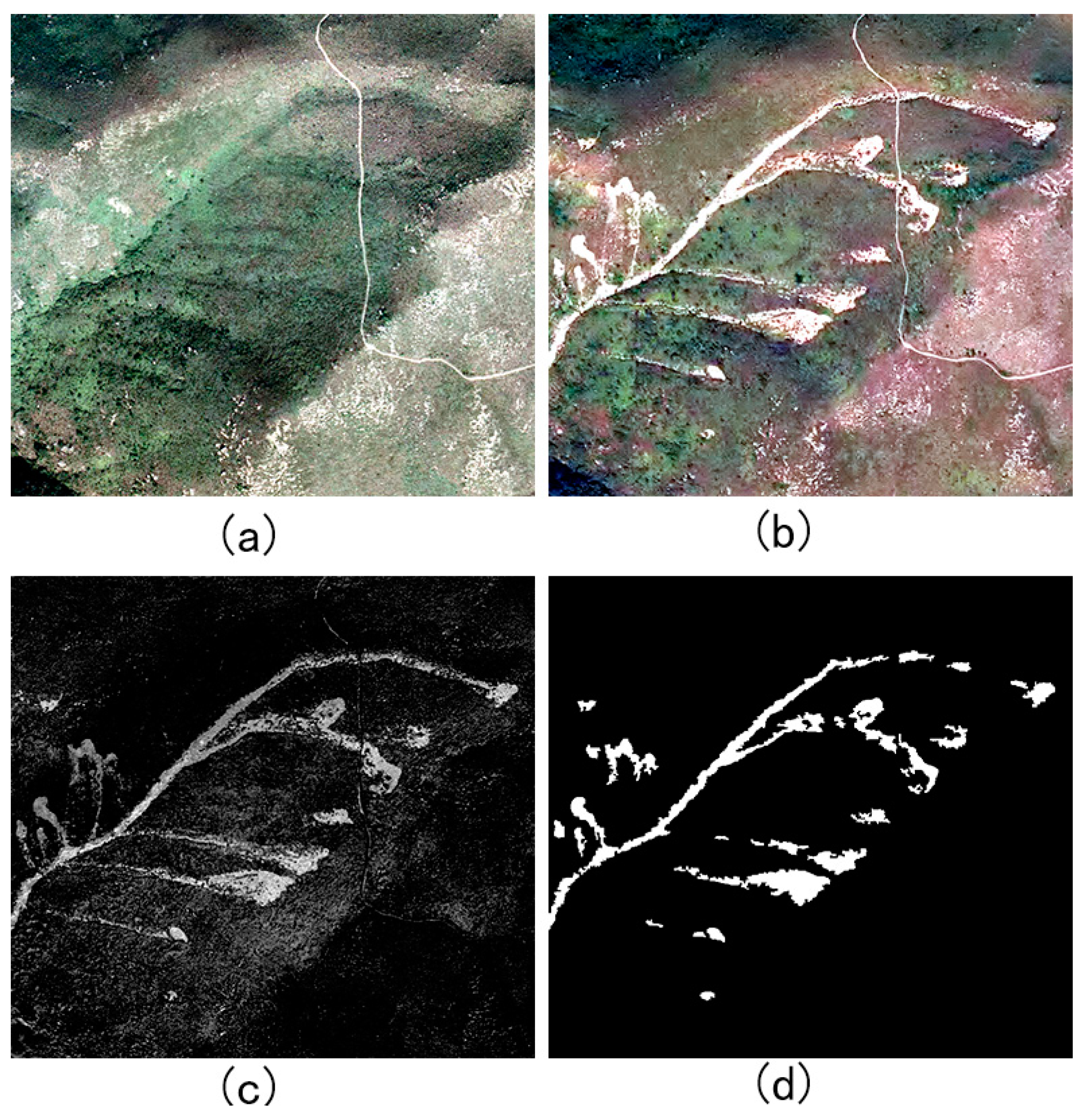
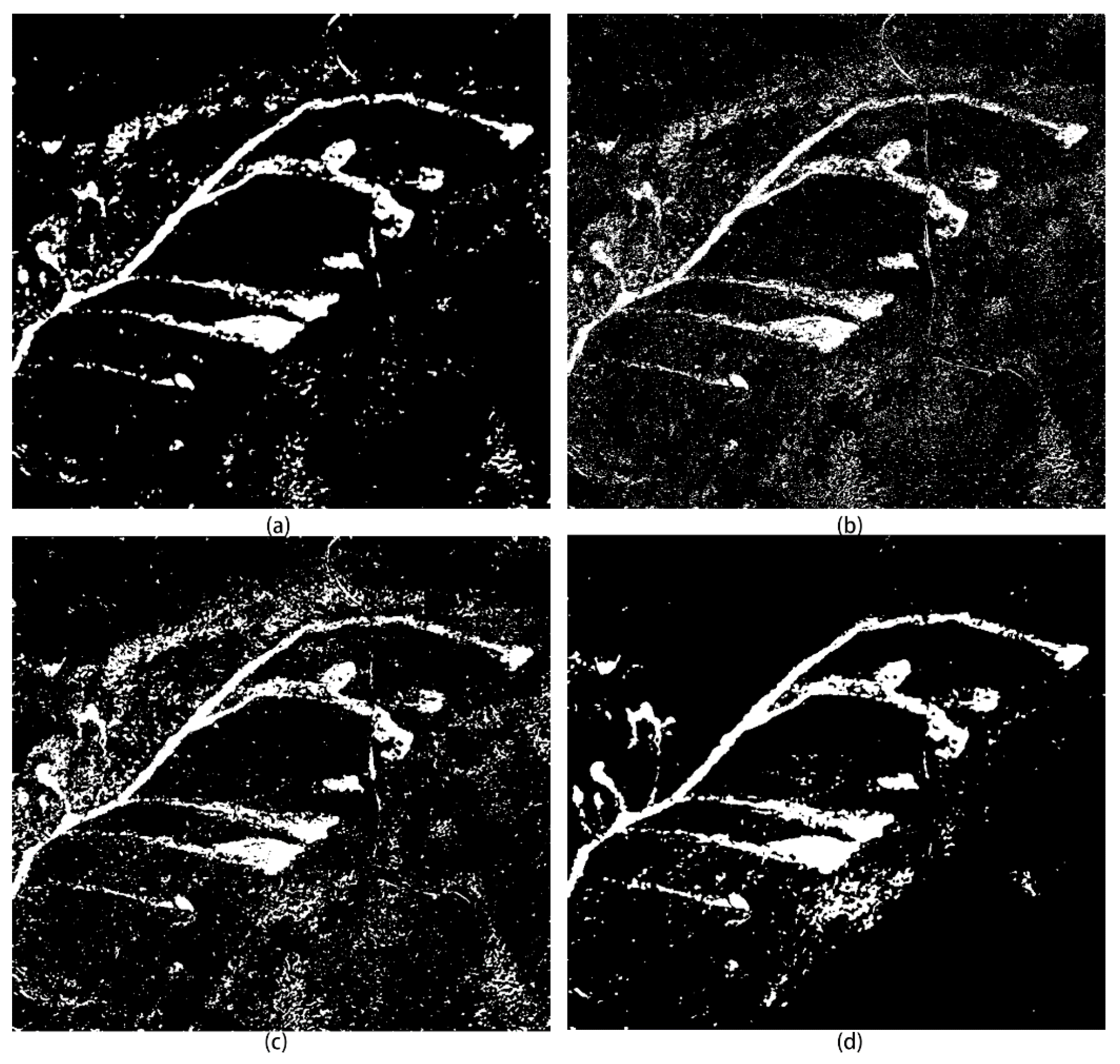
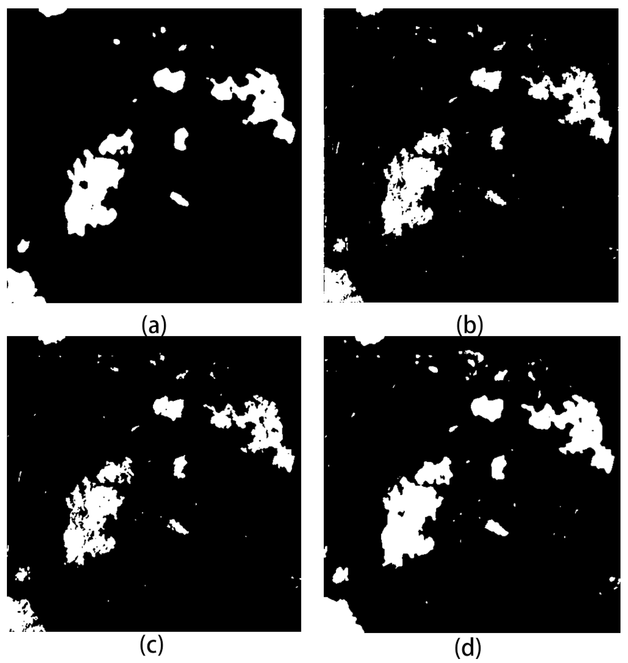
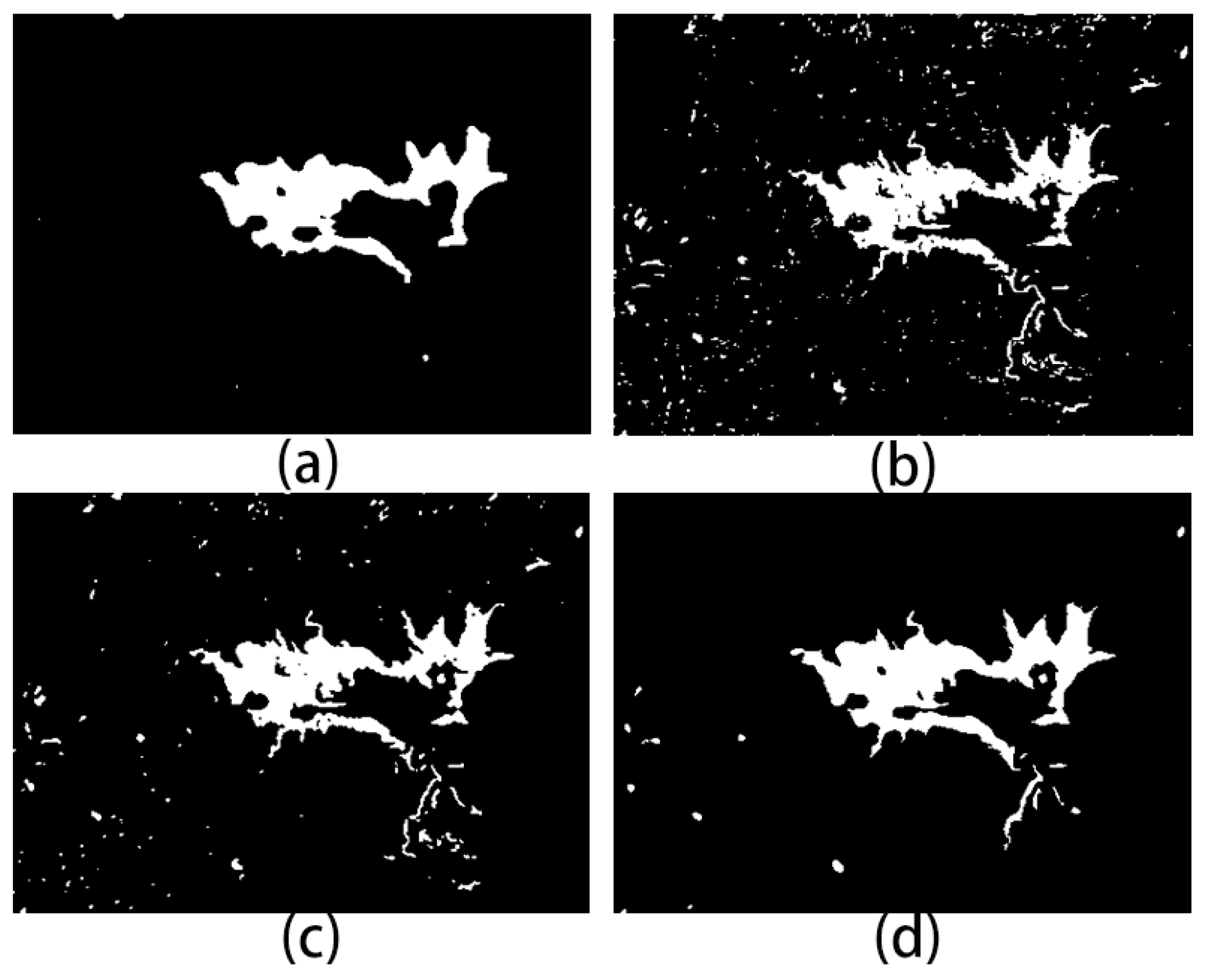
3.3. Results and Quantitative Evaluation
4. Discussion
5. Conclusions
Supplementary Materials
Acknowledgments
Author Contributions
Conflicts of Interest
References
- Celik, T. Unsupervised change detection in satellite images using principal component analysis and k-means clustering. IEEE Geosci. Remote Sens. Lett. 2009, 6, 772–776. [Google Scholar] [CrossRef]
- Bazi, Y.; Melgani, F.; Al-Sharari, H.D. Unsupervised change detection in multispectral remotely sensed imagery with level set methods. IEEE Trans. Geosci. Remote Sens. 2010, 48, 3178–3187. [Google Scholar] [CrossRef]
- Shao, P.; Shi, W.; He, P.; Hao, M.; Zhang, X. Novel approach to unsupervised change detection based on a robust semi-supervised fcm clustering algorithm. Remote Sens. 2016, 8, 264. [Google Scholar] [CrossRef]
- Giustarini, L.; Hostache, R.; Matgen, P.; Schumann, G.J.-P.; Bates, P.D.; Mason, D.C. A change detection approach to flood mapping in urban areas using terrasar-x. IEEE Trans. Geosci. Remote Sens. 2013, 51, 2417–2430. [Google Scholar] [CrossRef]
- Jin, S.; Yang, L.; Danielson, P.; Homer, C.; Fry, J.; Xian, G. A comprehensive change detection method for updating the national land cover database to circa 2011. Remote Sens. Environ. 2013, 132, 159–175. [Google Scholar] [CrossRef]
- Beuchle, R.; Grecchi, R.C.; Shimabukuro, Y.E.; Seliger, R.; Eva, H.D.; Sano, E.; Achard, F. Land cover changes in the brazilian cerrado and caatinga biomes from 1990 to 2010 based on a systematic remote sensing sampling approach. Appl. Geogr. 2015, 58, 116–127. [Google Scholar] [CrossRef]
- Homer, C.G.; Dewitz, J.A.; Yang, L.; Jin, S.; Danielson, P.; Xian, G.; Coulston, J.; Herold, N.D.; Wickham, J.; Megown, K. Completion of the 2011 national land cover database for the conterminous united states-representing a decade of land cover change information. Photogramm. Eng. Remote Sens. 2015, 81, 345–354. [Google Scholar]
- Li, Z.; Shi, W.; Lu, P.; Yan, L.; Wang, Q.; Miao, Z. Landslide mapping from aerial photographs using change detection-based markov random field. Remote Sens. Environ. 2016, 187, 76–90. [Google Scholar] [CrossRef]
- Li, Z.; Shi, W.; Myint, S.W.; Lu, P.; Wang, Q. Semi-automated landslide inventory mapping from bitemporal aerial photographs using change detection and level set method. Remote Sens. Environ. 2016, 175, 215–230. [Google Scholar] [CrossRef]
- Yang, H.; Dou, A.; Zhang, W.; Huang, S. Study on Extraction of Earthquake Damage Information Based on Regional Optimizing Change Detection from Remote Sensing Image. In Proceedings of the IEEE International Geoscience and Remote Sensing Symposium (IGARSS), Quebec, QC, Canada, 13–18 July 2014; pp. 4272–4275. [Google Scholar]
- Radke, R.J.; Andra, S.; Al-Kofahi, O.; Roysam, B. Image change detection algorithms: A systematic survey. IEEE Trans. Image Process. 2005, 14, 294–307. [Google Scholar] [CrossRef] [PubMed]
- Hussain, M.; Chen, D.; Cheng, A.; Wei, H.; Stanley, D. Change detection from remotely sensed images: From pixel-based to object-based approaches. ISPRS 2013, 80, 91–106. [Google Scholar] [CrossRef]
- Falco, N.; Dalla Mura, M.; Bovolo, F.; Benediktsson, J.A.; Bruzzone, L. Change detection in vhr images based on morphological attribute profiles. IEEE Geosci. Remote Sens. Lett. 2013, 10, 636–640. [Google Scholar] [CrossRef]
- Bruzzone, L.; Prieto, D.F. Automatic analysis of the difference image for unsupervised change detection. IEEE Trans. Geosci. Remote Sens. 2000, 38, 1171–1182. [Google Scholar] [CrossRef]
- Chen, J.; Lu, M.; Chen, X.; Chen, J.; Chen, L. A spectral gradient difference based approach for land cover change detection. ISPRS 2013, 85, 1–12. [Google Scholar] [CrossRef]
- Chen, J.; Chen, X.; Cui, X.; Chen, J. Change vector analysis in posterior probability space: A new method for land cover change detection. IEEE Geosci. Remote Sens. Lett. 2011, 8, 317–321. [Google Scholar] [CrossRef]
- Ghosh, A.; Mishra, N.S.; Ghosh, S. Fuzzy clustering algorithms for unsupervised change detection in remote sensing images. Inf. Sci. 2011, 181, 699–715. [Google Scholar] [CrossRef]
- Yuan, F.; Sawaya, K.E.; Loeffelholz, B.C.; Bauer, M.E. Land cover classification and change analysis of the twin cities (minnesota) metropolitan area by multitemporal landsat remote sensing. Remote Sens. Environ. 2005, 98, 317–328. [Google Scholar] [CrossRef]
- Lhermitte, S.; Verbesselt, J.; Verstraeten, W.W.; Coppin, P. A comparison of time series similarity measures for classification and change detection of ecosystem dynamics. Remote Sens. Environ. 2011, 115, 3129–3152. [Google Scholar] [CrossRef]
- Chen, X.; Chen, J.; Shi, Y.; Yamaguchi, Y. An automated approach for updating land cover maps based on integrated change detection and classification methods. ISPRS 2012, 71, 86–95. [Google Scholar] [CrossRef]
- Zhu, Z.; Woodcock, C.E. Continuous change detection and classification of land cover using all available landsat data. Remote Sens. Environ. 2014, 144, 152–171. [Google Scholar] [CrossRef]
- Seebach, L.; Strobl, P.; Vogt, P.; Mehl, W.; San-Miguel-Ayanz, J. Enhancing post-classification change detection through morphological post-processing–a sensitivity analysis. Int. J. Remote Sens. 2013, 34, 7145–7162. [Google Scholar] [CrossRef]
- Lu, D.; Mausel, P.; Brondizio, E.; Moran, E. Change detection techniques. Int. J. Remote Sens. 2004, 25, 2365–2401. [Google Scholar] [CrossRef]
- Huang, X.; Zhang, L.; Zhu, T. Building change detection from multitemporal high-resolution remotely sensed images based on a morphological building index. IEEE J. Sel. Top. Appl. Earth Obs. Remote Sens. 2014, 7, 105–115. [Google Scholar] [CrossRef]
- Huang, X.; Zhang, L. An svm ensemble approach combining spectral, structural, and semantic features for the classification of high-resolution remotely sensed imagery. IEEE Trans. Geosci. Remote Sens. 2013, 51, 257–272. [Google Scholar] [CrossRef]
- Subudhi, B.N.; Bovolo, F.; Ghosh, A.; Bruzzone, L. Spatio-contextual fuzzy clustering with markov random field model for change detection in remotely sensed images. Opt. Laser Technol. 2014, 57, 284–292. [Google Scholar] [CrossRef]
- Gu, W.; Lv, Z.; Hao, M. Change detection method for remote sensing images based on an improved markov random field. Multimed. Tools Appl. 2017, 76, 17719–17734. [Google Scholar] [CrossRef]
- Ghosh, A.; Subudhi, B.N.; Bruzzone, L. Integration of gibbs markov random field and hopfield-type neural networks for unsupervised change detection in remotely sensed multitemporal images. IEEE Trans. Image Process. 2013, 22, 3087–3096. [Google Scholar] [CrossRef] [PubMed]
- Volpi, M.; Tuia, D.; Bovolo, F.; Kanevski, M.; Bruzzone, L. Supervised change detection in vhr images using contextual information and support vector machines. Int. J. Appl. Earth Obs. Geoinf. 2013, 20, 77–85. [Google Scholar] [CrossRef]
- Lv, Z.Y.; Zhang, P.; Benediktsson, J.A.; Shi, W.Z. Morphological profiles based on differently shaped structuring elements for classification of images with very high spatial resolution. IEEE J. Sel. Top. Appl. Earth Obs. Remote Sens. 2014, 7, 4644–4652. [Google Scholar] [CrossRef]
- Huang, X.; Zhang, L.; Li, P. An adaptive multiscale information fusion approach for feature extraction and classification of ikonos multispectral imagery over urban areas. IEEE Geosci. Remote Sens. Lett. 2007, 4, 654–658. [Google Scholar] [CrossRef]
- Lv, Z.; Zhang, P.; Atli Benediktsson, J. Automatic object-oriented, spectral-spatial feature extraction driven by tobler’s first law of geography for very high resolution aerial imagery classification. Remote Sens. 2017, 9, 285. [Google Scholar] [CrossRef]
- Topouzelis, K.; Papakonstantinou, A.; Pavlogeorgatos, G. Coastline change detection using uav, Remote Sensing, GIS and 3D reconstruction. In Proceedings of the 5th International Conference on Environmental Management, Engineering, Planning and Economics (CEMEPE) and SECOTOX Conference, Mykonos Island, Greece, 14–18 June 2015. [Google Scholar]
- Tewkesbury, A.P.; Comber, A.J.; Tate, N.J.; Lamb, A.; Fisher, P.F. A critical synthesis of remotely sensed optical image change detection techniques. Remote Sens. Environ. 2015, 160, 1–14. [Google Scholar] [CrossRef]
- Liu, S.; Bruzzone, L.; Bovolo, F.; Du, P. Hierarchical unsupervised change detection in multitemporal hyperspectral images. IEEE Trans. Geosci. Remote Sens. 2015, 53, 244–260. [Google Scholar]
- Wen, D.; Huang, X.; Zhang, L.; Benediktsson, J.A. A novel automatic change detection method for urban high-resolution remotely sensed imagery based on multiindex scene representation. IEEE Trans. Geosci. Remote Sens. 2016, 54, 609–625. [Google Scholar] [CrossRef]
- Dalla Mura, M.; Benediktsson, J.A.; Bovolo, F.; Bruzzone, L. An unsupervised technique based on morphological filters for change detection in very high resolution images. IEEE Geosci. Remote Sens. Lett. 2008, 5, 433–437. [Google Scholar] [CrossRef]
- Wu, H.; Li, Z.-L. Scale issues in remote sensing: A review on analysis, processing and modeling. Sensors 2009, 9, 1768–1793. [Google Scholar] [CrossRef] [PubMed]
- Woodcock, C.E.; Strahler, A.H. The factor of scale in remote sensing. Remote Sens. Environ. 1987, 21, 311–332. [Google Scholar] [CrossRef]
- Townshend, J.R.; Justice, C.O.; Gurney, C.; McManus, J. The impact of misregistration on change detection. IEEE Trans. Geosci. Remote Sens. 1992, 30, 1054–1060. [Google Scholar] [CrossRef]
- Marchesi, S.; Bovolo, F.; Bruzzone, L. A context-sensitive technique robust to registration noise for change detection in vhr multispectral images. IEEE Trans. Image Process. 2010, 19, 1877–1889. [Google Scholar] [CrossRef] [PubMed]
- Cheng, K.; Wei, C.; Chang, S. Locating landslides using multi-temporal satellite images. Adv. Space Res. 2004, 33, 296–301. [Google Scholar] [CrossRef]
- Gong, M.; Zhan, T.; Zhang, P.; Miao, Q. Superpixel-based difference representation learning for change detection in multispectral remote sensing images. IEEE Trans. Geosci. Remote Sens. 2017, 55, 2658–2673. [Google Scholar] [CrossRef]
- Lee, J.-H.; Biging, G.S.; Fisher, J.B. An individual tree-based automated registration of aerial images to lidar data in a forested area. Photogramm. Eng. Remote Sens. 2016, 82, 699–710. [Google Scholar] [CrossRef]
- Zhang, L.; Li, A.; Zhang, Z.; Yang, K. Global and local saliency analysis for the extraction of residential areas in high-spatial-resolution remote sensing image. IEEE Trans. Geosci. Remote Sens. 2016, 54, 3750–3763. [Google Scholar] [CrossRef]
- Lv, Z.; Zhang, X.; Benediktsson, J.A. Developing a general post-classification framework for land-cover mapping improvement using high-spatial-resolution remote sensing imagery. Remote Sens. Lett. 2017, 8, 607–616. [Google Scholar] [CrossRef]
- Heijden, K.V.D. Image Based Measurement Systems; Fraunhofer IOSB: Karlsruhe, Germany, 2007. [Google Scholar]
- Sezgin, M. Survey over image thresholding techniques and quantitative performance evaluation. J. Electron. Imaging 2004, 13, 146–168. [Google Scholar]
- Otsu, N. A threshold selection method from gray-level histograms. IEEE Trans. Syst. Man Cybern. 1979, 9, 62–66. [Google Scholar] [CrossRef]
- Rosin, P.L.; Ioannidis, E. Evaluation of global image thresholding for change detection. Pattern Recognit. Lett. 2003, 24, 2345–2356. [Google Scholar] [CrossRef]
- Alesheikh, A.A.; Ghorbanali, A.; Nouri, N. Coastline change detection using remote sensing. Int. J. Environ. Sci. Technol. 2007, 4, 61. [Google Scholar] [CrossRef]
- Bovolo, F.; Bruzzone, L. A detail-preserving scale-driven approach to change detection in multitemporal sar images. IEEE Trans. Geosci. Remote Sens. 2005, 43, 2963–2972. [Google Scholar] [CrossRef]
- Gong, M.; Su, L.; Jia, M.; Chen, W. Fuzzy clustering with a modified mrf energy function for change detection in synthetic aperture radar images. IEEE Trans. Fuzzy Syst. 2014, 22, 98–109. [Google Scholar] [CrossRef]
- Levin, D. The approximation power of moving least-squares. Math. Comput. Am. Math. Soc. 1998, 67, 1517–1531. [Google Scholar] [CrossRef]
- Mao, F.; Gong, W.; Zhu, Z. Simple multiscale algorithm for layer detection with lidar. Appl. Opt. 2011, 50, 6591–6598. [Google Scholar] [CrossRef] [PubMed]
- Shi, W.; Hao, M. Analysis of spatial distribution pattern of change-detection error caused by misregistration. Int. J. Remote Sens. 2013, 34, 6883–6897. [Google Scholar] [CrossRef]
- Dai, X.; Khorram, S. The effects of image misregistration on the accuracy of remotely sensed change detection. IEEE Trans. Geosci. Remote Sens. 1998, 36, 1566–1577. [Google Scholar]
- Kasetkasem, T.; Varshney, P.K. An image change detection algorithm based on markov random field models. IEEE Trans. Geosci. Remote Sens. 2002, 40, 1815–1823. [Google Scholar] [CrossRef]
- Bruzzone, L.; Cossu, R. An adaptive approach to reducing registration noise effects in unsupervised change detection. IEEE Trans. Geosci. Remote Sens. 2003, 41, 2455–2465. [Google Scholar] [CrossRef]
- Stauffer, M.; McKinney, R. Landsat Image Differencing as an Automated Land Cover Change Detection Technique; Computer Sciences Corp.: Silver Spring, MD, USA, 1978. Available online: https://ntrs.nasa.gov/search.jsp?R=19830009647 (accessed on 10 September 2017).
- Singh, A. Tropical Forest Monitoring Using Digital Landsat Data in Northeastern India; University of Reading: Reading, UK, 1984. [Google Scholar]
- Fung, T.; LeDrew, E. The determination of optimal threshold levels for change detection using various accuracy indices. Photogramm. Eng. Remote Sens. 1988, 54, 1449–1454. [Google Scholar]
- Krylov, V.A.; Moser, G.; Serpico, S.B.; Zerubia, J. False discovery rate approach to unsupervised image change detection. IEEE Trans. Image Process. 2016, 25, 4704–4718. [Google Scholar] [CrossRef] [PubMed]
- Yetgin, Z. Unsupervised change detection of satellite images using local gradual descent. IEEE Trans. Geosci. Remote Sens. 2012, 50, 1919–1929. [Google Scholar] [CrossRef]


| Method | False Alarm | Missed Alarm | Overall Errors |
|---|---|---|---|
| CD_PCA_Kmeans | 4.34 | 12.46 | 4.76 |
| CD_MLS | 7.6 | 14.55 | 7.95 |
| Semi_FCM | 8.71 | 9.19 | 8.73 |
| The proposed | 3.29 | 7.03 | 3.48 |
| Method | False Alarm | Missed Alarm | Overall Errors |
|---|---|---|---|
| CD_PCA_kmeans | 2.52 | 19.47 | 3.35 |
| CD_MLS | 7.48 | 20.8 | 8.13 |
| Semi_FCM | 8.53 | 15.16 | 8.86 |
| The proposed | 1.87 | 17.90 | 2.66 |
| Method | False Alarm | Missed Alarm | Overall Errors |
|---|---|---|---|
| CD_PCA_Kmeans | 0.78 | 10.3 | 1.71 |
| CD_MLS | 0.58 | 11.9 | 1.68 |
| Semi_FCM | 0.41 | 15.0 | 1.83 |
| The proposed method | 1.08 | 4.73 | 1.43 |
| Method | False Alarm | Missed Alarm | Overall Errors |
|---|---|---|---|
| CD_PCA_Kmeans | 1.26 | 14.9 | 2.1 |
| CD_MLS | 2.64 | 9.83 | 3.09 |
| Semi_FCM | 1.77 | 9.86 | 2.27 |
| The proposed | 1.48 | 7.93 | 1.88 |
| Dataset | Binary Map Obtained by the Second Technique | Binary Map Optimized by the Third Technique | ||||
|---|---|---|---|---|---|---|
| False Alarm | Missed Alarm | Overall Errors | False Alarm | Missed Alarm | Overall Errors | |
| First Data | 3.85 | 8.40 | 4.30 | 3.29 | 7.03 | 3.48 |
| Second Data | 2.21 | 20.92 | 3.10 | 1.87 | 17.9 | 2.66 |
| Mexico | 1.12 | 5.23 | 2.24 | 1.08 | 4.73 | 1.43 |
| Sardinia Island | 1.51 | 10.20 | 2.00 | 1.48 | 7.93 | 1.88 |
© 2017 by the authors. Licensee MDPI, Basel, Switzerland. This article is an open access article distributed under the terms and conditions of the Creative Commons Attribution (CC BY) license (http://creativecommons.org/licenses/by/4.0/).
Share and Cite
Lv, Z.; Shi, W.; Zhou, X.; Benediktsson, J.A. Semi-Automatic System for Land Cover Change Detection Using Bi-Temporal Remote Sensing Images. Remote Sens. 2017, 9, 1112. https://doi.org/10.3390/rs9111112
Lv Z, Shi W, Zhou X, Benediktsson JA. Semi-Automatic System for Land Cover Change Detection Using Bi-Temporal Remote Sensing Images. Remote Sensing. 2017; 9(11):1112. https://doi.org/10.3390/rs9111112
Chicago/Turabian StyleLv, ZhiYong, WenZhong Shi, XiaoCheng Zhou, and Jón Atli Benediktsson. 2017. "Semi-Automatic System for Land Cover Change Detection Using Bi-Temporal Remote Sensing Images" Remote Sensing 9, no. 11: 1112. https://doi.org/10.3390/rs9111112
APA StyleLv, Z., Shi, W., Zhou, X., & Benediktsson, J. A. (2017). Semi-Automatic System for Land Cover Change Detection Using Bi-Temporal Remote Sensing Images. Remote Sensing, 9(11), 1112. https://doi.org/10.3390/rs9111112