Application of Low-Cost UASs and Digital Photogrammetry for High-Resolution Snow Depth Mapping in the Arctic

Abstract

The repeat acquisition of high-resolution snow depth measurements has important research and civil applications in the Arctic. Currently the surveying methods for capturing the high spatial and temporal variability of the snowpack are expensive, in particular for small areal extents. An alternative methodology based on Unmanned Aerial Systems (UASs) and digital photogrammetry was tested over varying surveying conditions in the Arctic employing two diverse and low-cost UAS-camera combinations (500 and 1700 USD, respectively). Six areas, two in Svalbard and four in Greenland, were mapped covering from 1386 to 38,410 m². The sites presented diverse snow surface types, underlying topography and light conditions in order to test the method under potentially limiting conditions. The resulting snow depth maps achieved spatial resolutions between 0.06 and 0.09 m. The average difference between UAS-estimated and measured snow depth, checked with conventional snow probing, ranged from 0.015 to 0.16 m. The impact of image pre-processing was explored, improving point cloud density and accuracy for different image qualities and snow/light conditions. Our UAS photogrammetry results are expected to be scalable to larger areal extents. While further validation is needed, with the inclusion of extra validation points, the study showcases the potential of this cost-effective methodology for high-resolution monitoring of snow dynamics in the Arctic and beyond.

1. Introduction

In Arctic regions, the spatiotemporal variability of the snowpack plays a critical role in local climate, hydrological and ecological systems [1,2]. Accurate, spatially resolved estimations of snow depth over scales of a few meters to landscapes covering several thousands of m² are valuable for an array of applications ranging from environmental research to civil purposes.

Specific examples include (i) the detection of snow depth variability across small-scale landscape topography required in terrestrial ecosystems research [1,3,4], (ii) the monitoring and diagnosis of permafrost conditions [5,6], (iii) development of numerical models and retrieval algorithms for remote sensing of sea-ice properties and ecosystem research [7,8], and (iv) generation of local snow depth distribution predictive models and for their validation [9,10,11]. Finally, for civil engineering applications, information on the small-scale evolution of the snowpack is useful for avalanche prediction [12,13] and snow drift modeling around buildings [14].

Accurate and spatially continuous measurements of snow depth are challenging due to the high spatial and temporal variability at different spatial scales [11,15]. Increased variability is also characteristic of observing snow depth at finer mapping scales and for shallower areas. In the Arctic, seasonal snow cover is present for most of the year due to the low temperature and shorter melting season. Strong winds and scarce snowfall produce a snow cover that is typically quite shallow and much more variable in space (about 30–40 cm except in drifts and gullies) and time (hourly and daily) [16] compared to thicker alpine snowpack.

Capturing this variability, particularly under complex underlying topographies, requires easily repeatable and increased resolution estimates [1,11,17].

Various techniques have been developed over the last century to monitor snow depth, each one presenting a characteristic set of advantages and limitations. Point or line measurements of snow depth using probing or ground penetrating radar both give spatially incomplete measurements, cannot be automated, cannot be used in steep slopes or avalanche/hazard risk zones, and are not suitable for the characterization of decimeter-scale variability beyond plot scale [18].

Snow pillows or sonic rangers are fully automated but give point measurements with questionable representativeness [19,20]. Outside the range of satellite remote sensing products that are aimed at large regional and catchment wise applications, airborne or terrestrial Light Detection and Ranging (LiDAR) is the most advanced technique. LiDAR is capable of accurately mapping continuous swaths of snow depth for large areal extents and at high spatial resolutions depending on the approach taken, e.g., aerial or terrestrial [18,21]. However, if small areas are to be surveyed, airborne LiDAR techniques come at relatively high cost, and require specific equipment and a certain level of expertise both in the survey and data processing phase. This makes them of limited use considering the wide, logistically limiting, and sparsely populated Arctic.

In this context, this work aims to assess a procedure combining Unmanned Aerial Systems (UASs) with Structure from Motion (SfM) digital photogrammetry, as a cost- and labor-efficient technique capable of capturing the spatial distribution of snow depth for a range of different Arctic surveying conditions.

SfM is capable of reconstructing 3D models of topography from a set of overlapping pictures acquired with consumer grade digital cameras [22,23]. The 3D models can then be georeferenced using a set of Ground Control Points (GCPs) with known geographic positions producing a Digital Elevation Model (DEM) [24]. If digital cameras are equipped on aerial platforms such as manned or Unmanned Aerial Systems (UASs), considerable areal extents can then be covered at a reduced effort, making it an effective tool from a geosciences perspective [24,25].

Recent studies have shown the potential of UAS-borne SfM for snow mapping [26,27,28,29]. The method consists of the subtraction of an underlying topography DEM (TDEM) from its SfM-generated snow surface cover DEMs (SDEMs). Snow surface reconstruction with SfM is, however, considered problematic due to the lack of texture (lack of image contrast) in the acquired photographs, which hampers the algorithm’s ability to feature-track, identify, and match pictures [23,24,30]. As image texture is heavily influenced by the snow surface type (e.g., fresh, wind-packed, etc.), more investigation is required to assess the impact of snow’s physical properties on SDEM reconstructions [26,28]. In addition, light (luminance) is also very important for the SfM workflow as it enhances the ability to discriminate fine detail by augmenting image contrast [31]. Light availability consequently affects the ability of the method to perform over a range of sky conditions (e.g., flat lighting due to overcast sky) and requires further testing [28,29]. Beyond the need to test the methodology under different surveying conditions, considerable improvements can be made with sensor choice (resolution, payload weight, and cost trade-offs) and workflow optimization (e.g., in image acquisition and pre-processing) [26]. These are particularly important at high latitudes where there are reduced operational windows and high logistical costs.

The aim of this study was to assess the feasibility of UAS-SfM for capturing Arctic snow depth variability at high resolutions and for a set of the aforementioned challenging scenarios.

Tests were conducted using two different budget UAS-camera solutions (<1700 USD) deployed at two sites near Longyearbyen, Svalbard and at four sites near Sisimiut, West Greenland.

Multiple sites suited the overall objective of investigating the applicability of this method under a range of different mapping scenarios that are suspected to be detrimental for its performance and require further scientific effort. These include diverse snow surface types, light availability, and underlying topography complexity. Multiple payloads suited the aim of further optimizing the method from a procedural and cost perspective.

The specific objectives can be summarized as follows:

(1)

Investigating improved workflow solutions in the image pre-processing phase aiming to boost SfM reconstruction performances and correct systematic errors.

(2)

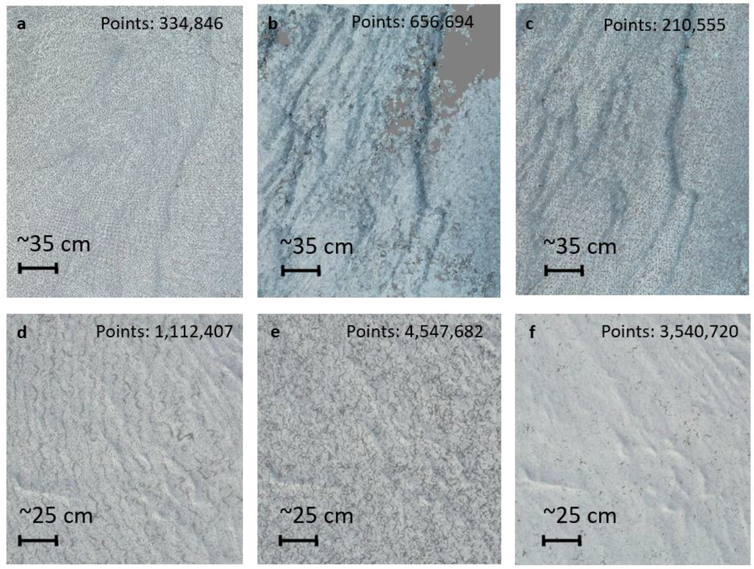
Assessing the effect of lighting conditions, snow surface type, and camera equipment on the SDEM generation process. This includes investigating the achievable spatial resolutions for each case with the tested equipment.

(3)

Evaluating the overall feasibility and performance of the proposed low-cost method to capture snow depth variability for different underlying topographies. This is done by a comparison of the snow depth estimates with traditional snow probing and over snow-free areas.

The study concludes with a discussion of these relatively low-cost set-ups as an efficient alternative to track the high spatial variability of snow depth over contained areal extents in the challenging Arctic environment.

2. Study Areas and Survey Conditions

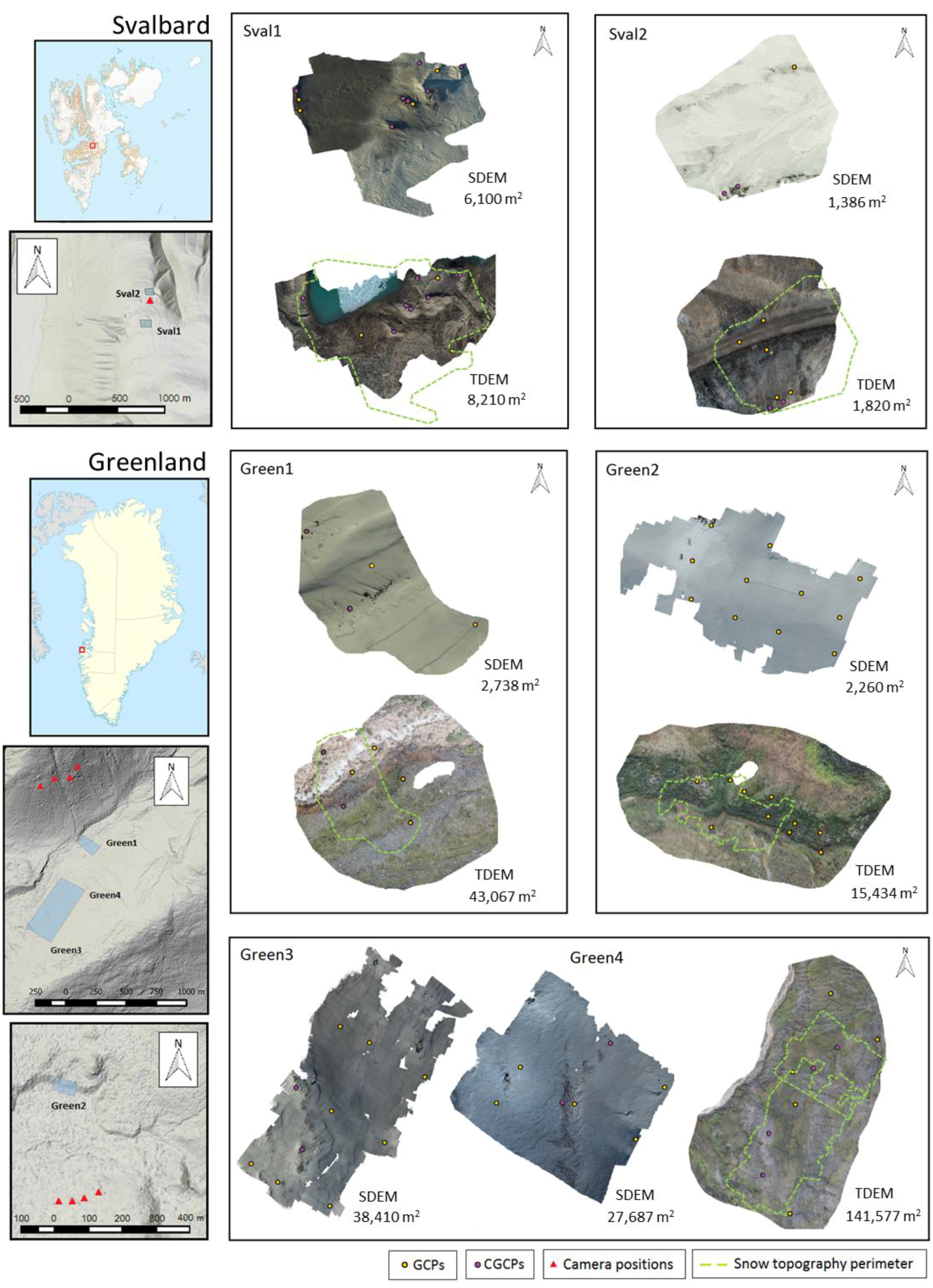
Six assorted snow-covered areas were mapped to produce SDEMs during late-winter conditions in April 2015. The surveyed areas differed in terms of snow surface pattern type, light conditions, and underlying topography complexity. The areas were resurveyed in July 2015 during summer conditions to provide TDEMs. The geographical location of the sites is shown in Figure 1, with conditions at each site summarized in

Table 1. Surveying conditions and general characteristics of the six surveyed areas. Two areas are located in Svalbard (Sval1 and Sval2) and four in Greenland (Green1–4). The physiography descriptors are summarized in the form of topography/terrain type. The influencing surveying conditions tested are listed in the form of luminance (light) conditions and snow surface type. SDEM and TDEM refer to snow and terrain DEMs, respectively. GCPs stands for the amount of ground control points used for georeferencing each surface. CGCPs stands for co-ground control points as the number of shared GCPs in the co-georeferencing process between snow and terrain topography.

Area Name	Coordinates (Lat/Lon in WGS 84)	Survey Date (dd/mm/yyyy)		Luminance Conditions	Snow Surface Type	Physiography Descriptors	Number of GCPs		CGCPs
		SDEM	TDEM	SDEM	SDEM	TDEM	SDEM	TDEM
Sval1	78°09′23″N	5/April/2015	6/July/2015	Overcast/Fair	Sastrugi	Horizontal but complex, irregular and variable surface with several bumps reliefs/Rock and ground debris	11	10	7
	16°01′57″W
Sval2	78°09′34″N	9/April/2015	8/July/2015	Overcast	Sastrugi and snow dusting	Steep slope next to man-made road/Bare soil and rock debris	3	7	2
	16°02′04″W
Green1	67°10′53″N	24/April/2015	28/July/2015	Fair	Fresh and smooth	Terrain ridge at edge of torrent/Rock debris and sparse low vegetation (5 to 15 cm)	4	6	2
	53°14′07″W
Green2	67°06′56″N	25/April/2015	27/July/2015	Clear Sky	Wind packed and smooth	Steep slope/Soil and both low and thick vegetation (10 to 30 cm)	11	10	0
	53°19′19″W
Green3	67°10′35″N	25/April/2015	28/July/2015	Clear Sky	Smooth with light snow ripples	Highly heterogeneous and variable topography reliefs/Soil, boulders, rock debris, and low vegetation (5 to 15 cm)	10	9	2
	53°14′34″W
Green4	67°10′40″N	26/April/2015	28/July/2015	Fair/Clear Sky	Sastrugi and light snow ripples		7		2
	53°14′22″W

. Snow surface type, luminance conditions, and topography complexity were qualitatively defined during all surveys (examples shown in Figure 2a–e).

2.1. Svalbard Areas

Two of the study sites were located in Breinosa, approximately 12 km east of Longyearbyen, Svalbard (Sval1 and Sval2, Figure 1). Their snowpack consisted of compacted wind-blown snow with small sastrugis features that were 1 to 10 cm wide (Figure 2b). No additional snowfall was recorded on the days prior to the survey date. The Sval1 terrain site is relatively flat but presented well-defined bumps that accumulated drifting snow on its lee side, producing a complex and irregular snowpack (Figure 2b). The Sval1 terrain was located near an artificial lake and consisted of bare soil and rock debris. The smaller site of Sval2 consisted of a steep north-facing slope next to a terrain vehicle road. Again, the terrain beneath the snowpack mainly consisted of bare soil and rock debris. Light conditions for both Sval1 and Sval2 surveys had consistent cloud cover, producing a flat and low light scenario (Figure 2a–c).

2.2. Greenland Areas

The other four sites (Green1–4) were located approximately 30 km northeast of Sisimiut in the Kangerluarsuk Tulleq area, West Greenland (Figure 1), near the Sisimiut hydropower plant. In contrast with the Svalbard campaigns, the Greenland winter campaign was preceded by 15 mm of water equivalent snowfall, which, along with low speed winds (2 to 3 m s⁻¹), resulted in much smoother and more featureless snow surface (Figure 2d,e). However, areas Green3 and Green4 were subject to moderate winds on the night prior to the surveys, which produced light snow ripples on the surface.

Green1 is a northwest-facing soil terrain ridge at the edge of a glacier torrent with some rock debris and sparse vegetation. In contrast, Green2 faces south and has moderately steep relief that is mostly characterized by thick (10 to 30 cm) vegetation-covered topography near the slope base (Figure 2f). Green3 and Green4 are two relatively big areas in close proximity on the side of a glacier valley with a highly heterogeneous topography consisting of soil, boulders of variable sizes (up to 4 m), rock debris, and low vegetation (similar to Figure 2f). All surveys in Greenland were conducted on fair to sunny days with fast-moving clouds leading to variable lighting conditions (Figure 2d,e). The topographies of all areas are shown in the orthomosaics in Figure 1.

3. Materials and Methods

During the winter surveys (SDEMs), two different low-cost experimental setups were tested comprising different payload and image quality parameters (e.g., weight, resolution, geometrical distortion, etc.). Hereafter we refer to these as the minimal and advanced set-ups, respectively. During the summer surveys (TDEMs), Sval1 site was investigated using UAS-borne SfM while Sval2 and Green1–4 were surveyed using land-based SfM (pictures were taken from viewpoints overlooking the study site) due to a UAS failure. The land-based nature of the SfM generated terrain DEMs is not considered detrimental to this study objective as one of the primary goals is to demonstrate the capability of SfM to map different types of snow cover.

The UAS, camera models, and lenses used for each surveyed area are summarized in

Table 2. Summary of the equipment used for each mapped area and the relevant mapping parameters. SDEM and TDEM refer to both snow and terrain DEM, respectively. Automatic * refers to the fact that the GoPro^® Hero 3 does not allow any customization of the settings. Variable* refers to the variable nature of the exposures selected during the land-based survey. Shooting distance refers to the approximate camera position distances during the land-based SfM surveys (analogue to flying altitude). Camera settings include focal length range used for each image sub-set, aperture, shutter speed, and ISO settings, respectively.

Area Name	UAS Set-Up or Land-Based Survey		Average Flying Altitude or Shooting Distance Range (m)		Camera Settings		Acquired Images
	SDEM	TDEM	SDEM	TDEM	SDEM	TDEM	SDEM	TDEM
Sval1	Minimal set-up	Advanced set-up	7	23	2.77 mm f/2.8 Automatic *	18 mm	909	194
						f/4.5
						1/3200 s
						200
Sval2		Land-based SfM with Nikon D3200	8	2–10		18–34 mm Variable *	246	45
Green1			7	300–350		92–300 mm Variable *	873	153
Green2	Advanced set-up		11	300–500	18 mm	110–300 mm Variable *	160	120
					f/8.0
					1/3200 s
					100
Green3			20	700–1500	18 mm	59–300 mm Variable *	818	89
Green4			26		f/18		709
					1/800 s
					100

. The entire methodology of the study is schematized in Figure 3. Relevant aspects for each step are described in this section along with the equipment/software used.

3.1. UAS Set-Ups

3.1.1. Minimal Set-Up

For SDEM mapping of Sval1, Sval2 and Green1 we employed a Walkera X350 Pro quadcopter and a lightweight GoPro^® Hero 3 (payload weight of 150 g in total) (seen in Figure 2a). The GoPro^® Hero 3 was the silver edition model with an 11 megapixel sensor (3840 × 2880 pixels). The camera is mounted on a motorized stabilization gimbal that allows changes to the viewing angle and dampens rotor-induced vibrations.

GoPro^® does not allow any customization of its settings and has a fixed lens and aperture with automatic ISO and shutter speed. The total weight of this UAS set-up is 1.5 kg and embodies the minimal equipment (~500 USD) necessary to perform aerial SfM. The flight durability is 15–20 min per standard LiPO battery.

3.1.2. Advanced Set-Up

Higher quality images benefit the SfM procedure and lead to a better end product. However, carrying a better and more tunable camera comes with a payload weight that likely requires an upgrade of the UAS. This means more overhead with equipment costs, flight endurance, regulations, and pilot certification (Appendix A). To investigate the relative value of using a more advanced UAS set-up, the snow-covered areas Green2, Green3, and Green4 were surveyed with a Nikon D3200 DSLR camera with a NIKKOR 18–55 mm lens (payload weight of 790 g in total), mounted on a DJI s900 hexacopter. The payload was mounted in a custom-built gimbal that dampens the rotors’ vibration and allows for tilting of the gimbal angle (Appendix B). The Nikon D3200 sensor has a resolution of 24.2 effective mega-pixels (6016 × 4000 pixels) and was triggered with a Polaroid intervalometer for setting the timing of image acquisition. The total weight of this UAS system was approximately 4.2 kg and cost around 1700 USD. In the current experiments, the Nikon D3200 lens focus was always set to infinity and the focal length was generally set around 18–20 mm, which provided the widest footprint possible at a given altitude with the available lens. This represents a more complex high-end solution in terms of flying difficulty and camera set-up and flying times are noticeably reduced to 7–10 min compared to the minimal set-up.

The summer conditions mapping of Sval1 area used a custom-built octocopter together with the Nikon D3200 attached with the same gimbal used with the DJI s900. This UAS set-up cost around 1000 USD, camera included. This set-up is considered analogous to the advanced set-up as camera and settings were unchanged.

3.2. UAS Surveys

The UAS surveys were performed in agreement with local regulations for each case. A brief overview of the regulations of flying UAS in the Arctic can be found in Appendix A. The initial aim was to acquire millimeter-scale resolution imagery so datasets can then be downscaled to the maximum practical point that yielded desirable spatial resolution from a snow variability context. The SDEM generation was divided into four chronological steps (Figure 3): (1) allocation of GCPs on the survey site, (2) UAS-borne image acquisition, (3) GNSS survey of the GCPs, and (4) manual snow depth probing.

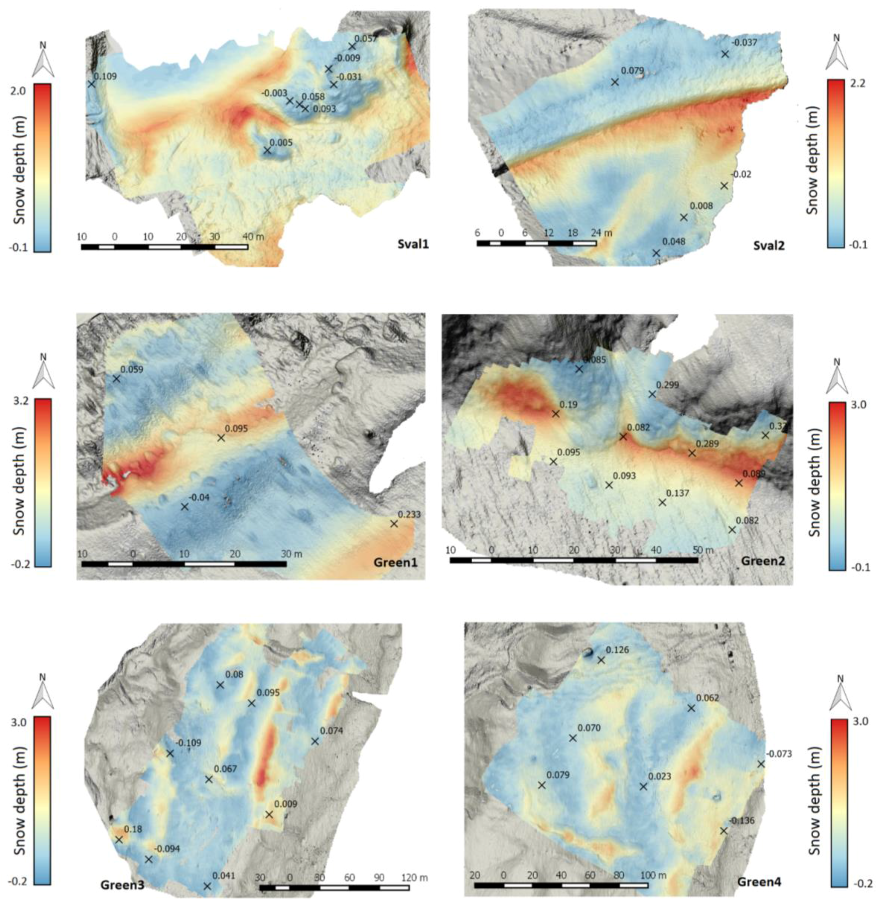
• Allocation of GCPs. GCPs are required for georeferencing the reconstructed 3D model [22,23]. The GCPs were distributed across the surveyed area as widely as possible [32]. All GCPs had a distinctive mark on their surface to precisely pinpoint the GCP on the imagery. They consisted of hand-made targets (circular plates with a centered red-cross) and snow-free features (e.g., overlying boulders, rocks, and ground patches) during winter. During summer, GCPs consisted of easily identifiable marked rocks. Features on snow-free areas, termed co-ground control points (CGCPs), are selected in support of co-georeferencing the SDEMs with the TDEMs [26]. The number of GCPs and CGCPs for each area are listed in Table 1 and positions can be seen in Figure 1. GCPs were carefully deployed to keep the majority of the snow undisturbed. This limited the addition of unnatural features in the snow that could unfairly assist the SfM reconstruction [26].
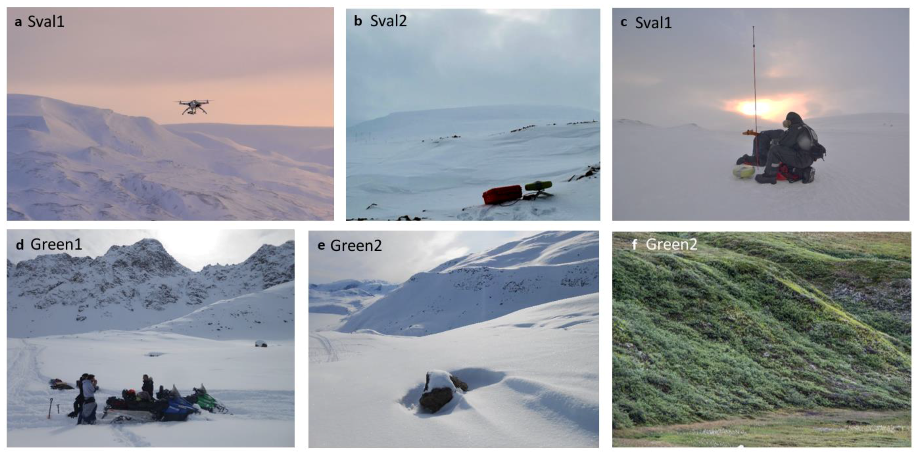
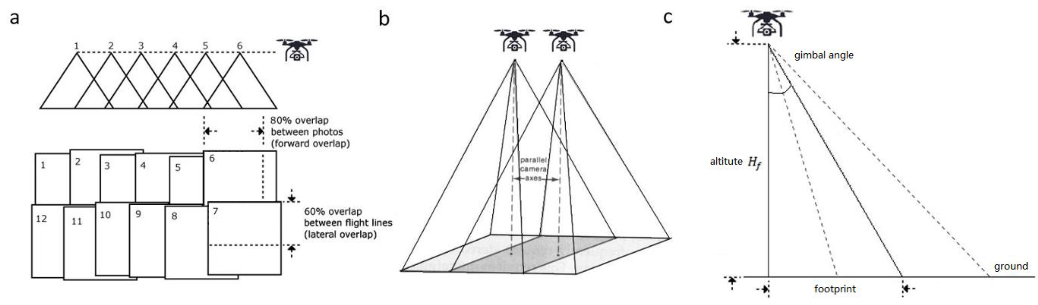
• UAS-borne image acquisition. With the aim of achieving millimeter-scale ground sample distance (GSD), the UAS flying parameters (altitude and speed) and the camera internal parameters (focal length and exposure) were set according to the local surveying characteristics (area extent and environment conditions shown in Table 2) using standard photogrammetric formulas (Appendix B). Millimeter-scale GSD is needed to ensure the downscaled (resampled) image resolution is sufficient to produce DEMs of the variable snow surfaces at the optimal scale. The guidelines and formulas for calculating typical UAS mapping parameters are found in Appendix B. The image acquisition frequency was set to 1 image per second. Once the cameras were configured for each surveyed area, the UAS was flown with a typical systematic mapping pattern with the camera directed orthogonal to the surface (Figure 2a and Appendix B). Additionally, as suggested by [33], a set of slightly oblique imagery is taken for each area by tilting the camera gimbals of ~ 20 degrees from vertical. With this setting, two additional flight transects were conducted for each area with the tilted camera pointing towards the center [33]. The ratio oblique/orthogonal imagery resulted to be around 0.2. Oblique imagery yields an increased ground footprint (Appendix B). Overall, this resulted in a high mean image overlap for the smaller areas mapped with the minimum set-up of Sval1 (>9 for SDEM), Sval2 (9) and Green1 (>9). Areas mapped with the advanced set-up resulted in a medium image overlap of Sval1 (8 for TDEM), Green2 (6), Green3 (8) and Green4 (7). The Nikon D3200 utilized the RAW-file format, i.e., non-compressed data from the camera sensor, which allowed a wider range of post-processing possibilities. The GoPro^® Hero 3 compressed the images to JPEG-file format.
• GNSS survey of the GCPs. For the positioning of the GCPs and of a few additional snow depth samples (3 for area Sval2 and 1 for area Green4, taken post-survey), a static GNSS survey was carried out with a JAVAD Legacy receiver and a JAVAD RegAnt antenna (Figure 2b). The geometric center of the antenna was aligned with the center of the GCP marker (red cross midpoint). In cases of irregular topography, we took repeat measurements of the distance from the snow surface to the antenna measuring point and used the average for determining the antenna height. The static GNSS acquisition times ranged from 30 to 90 min with a 1 Hz frequency. Satellites from both the GPS and the GLONASS systems are used in the positioning process.
• Snow depth survey. Snow depth was probed at the GCP and samples positions, repeated five times with a 3 m long avalanche probe marked with a cm scale (Figure 3c). The probing was initially performed directly below the mark of the circular red-crossed plates and thereafter four times around them to validate the snow depth measurement. Multiple measurements were needed to assess the presence of small ground irregularities under the snow cover.

3.3. Land-Based Surveys

Due to technical issues with the UAS platform, compounded by the remoteness of the area, Sval2 and Green1–4 were mapped during summer conditions as land-based SfM using the Nikon D3200 [23,34]. A NIKKOR 18–55 mm lens was used for Sval2 whereas a NIKKOR 55–300 mm was used for Green1–4. The procedure is analogous to the snow surveys excluding the snow depth survey. Images were acquired from higher-ground viewpoints on the valley sides opposite the study sites.

The approximate shooting distance is specified in Table 2 and camera positions are shown in Figure 1. Camera positions from a greater distance require a higher zooming range to achieve comparable resolutions. A NIKKOR 55–300 mm telephoto zoom lens was used to achieve a pixel size comparable to the winter campaigns of Green1–4. The focal length throughout the image acquisition was kept constant when possible. When unavoidable, different image sets using the same focal length were acquired. These sets could be then be reconstructed as separate chunks and be merged together into Photoscan Pro [35].

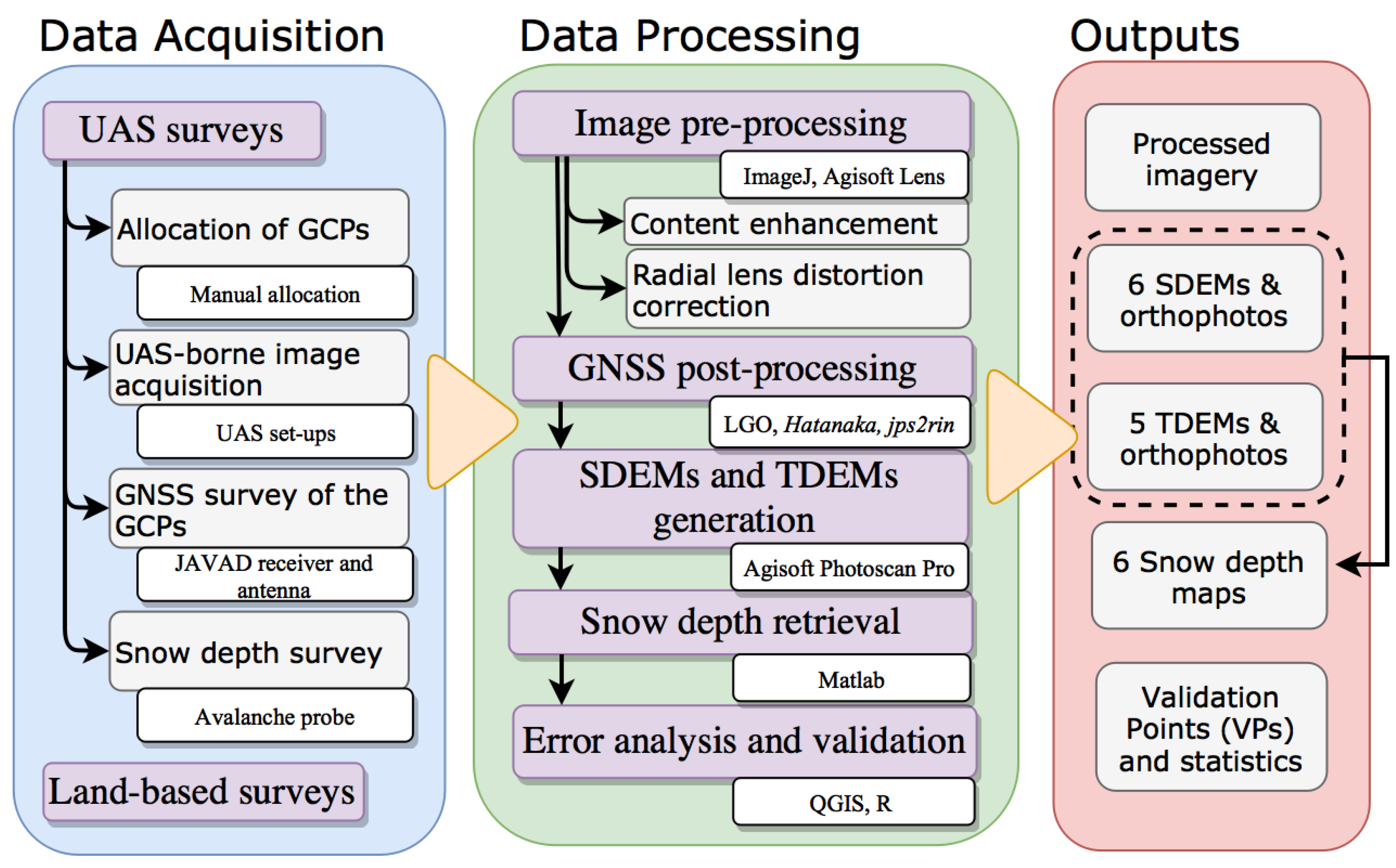
3.4. Data Processing

A five-step data processing workflow was performed for each of the surveyed areas(Figure 3): (1) snow imagery pre-processing (2) GNSS post-processing of GCP data, (3) Agisoft Photoscan Pro SDEMs and TDEMs generation [35], (4) snow depth calculation, and (5) error analysis and validation.

3.4.1. Snow Imagery Pre-Processing

Manual image pre-selection was done to remove blurred images. These images are often the result of wind-driven instabilities causing abrupt maneuvers or sudden changes in UAS altitude. The aim of the pre-processing phase was to explore the potential of image manipulation on the SDEM generation process and to enhance the photogrammetric reconstruction performance over typically featureless and homogenous snow surfaces. Pre-processing approaches for SfM have proven successful for improved 3D model reconstructions in other disciplines [31]. Another aim was to assess and correct the effects of systematic errors arising from DEM generation with nadiral and/or wide angle acquired imagery, in particular in this application where the subtraction of two UAS generated DEMs could introduce undesired effects [33]. The pre-processing solution was tested and implemented in two steps, (1) image content enhancement and (2) radial lens distortion correction.

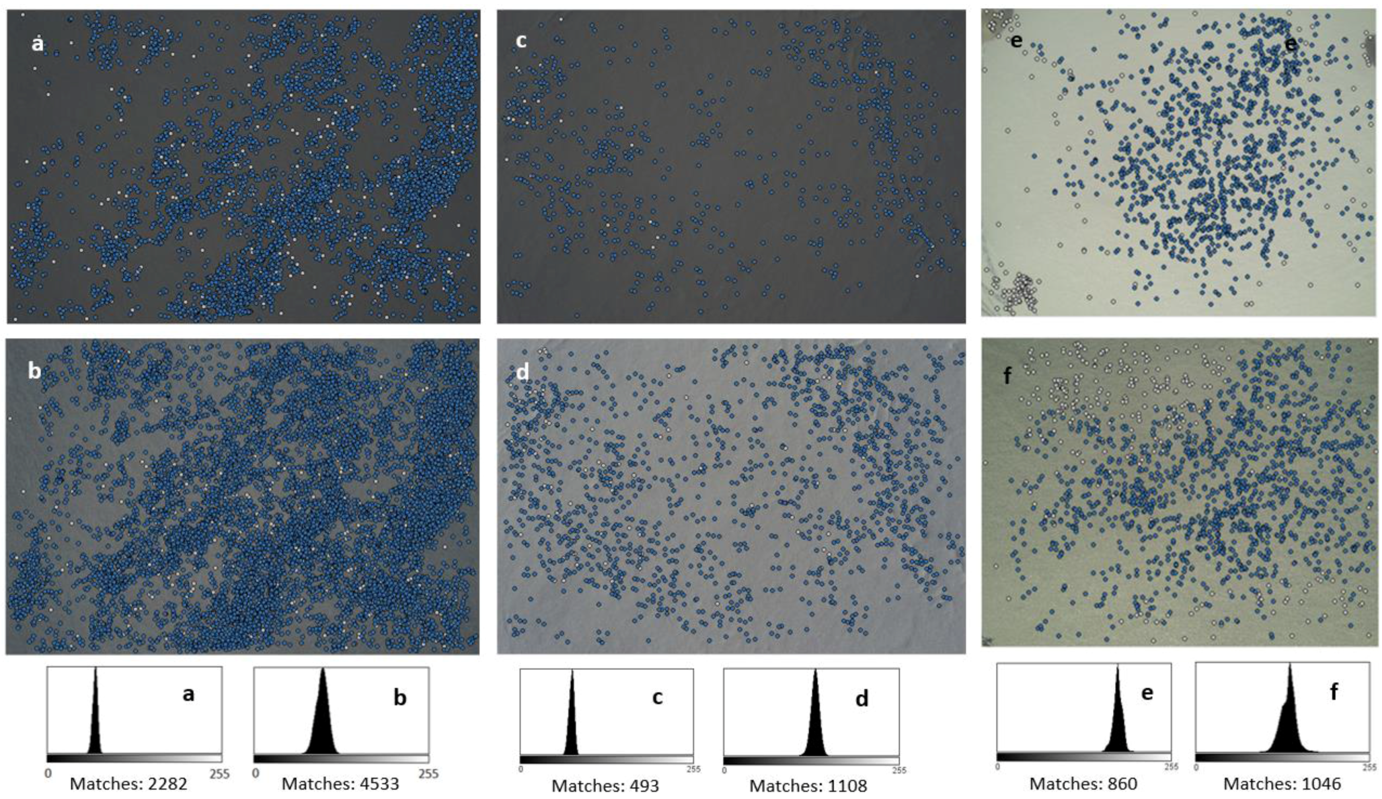
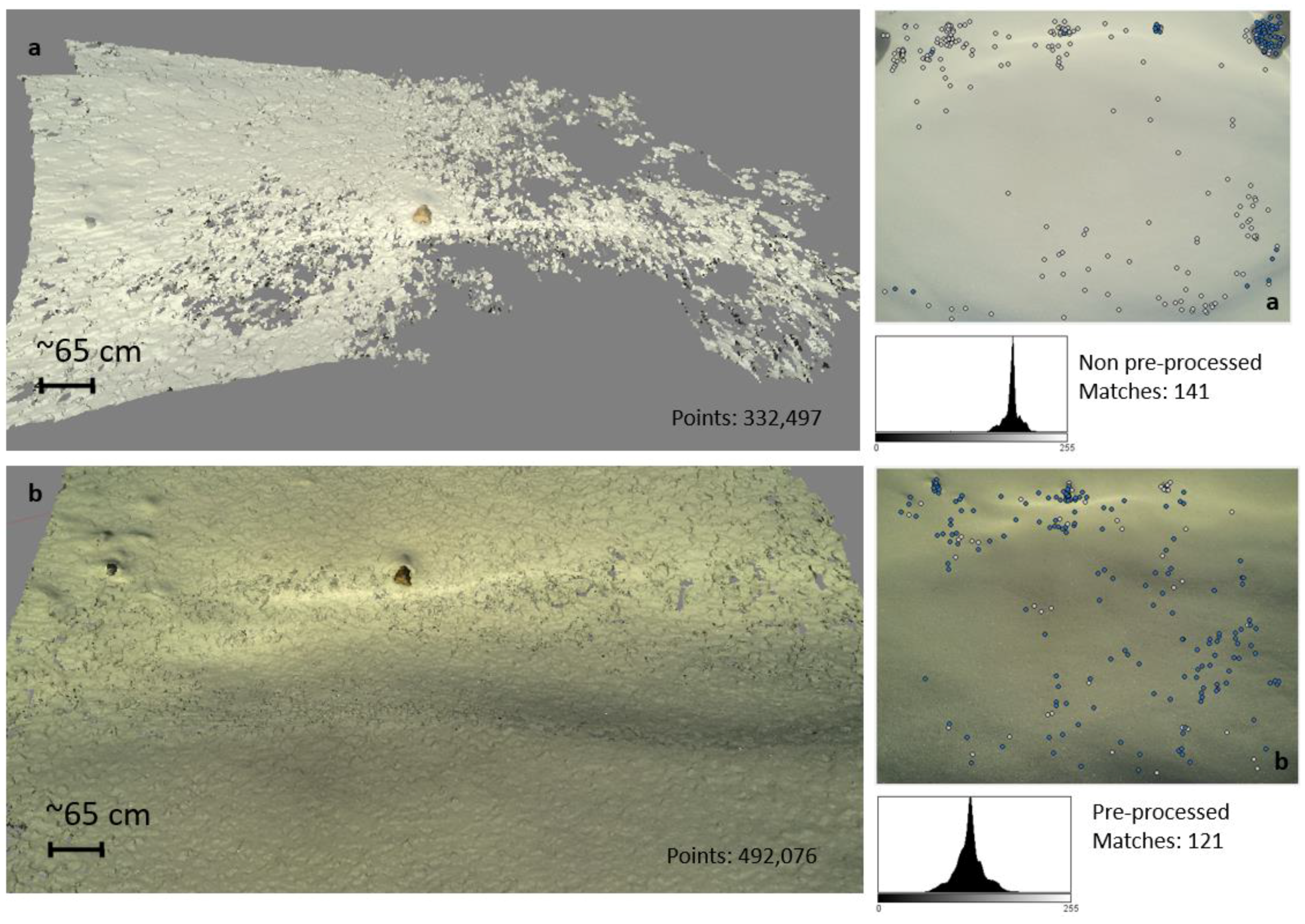
• Content enhancement. Image contrast, defined as the difference in luminance (light) intensity between an image’s object and background [36], is central to feature tracking algorithms. This is because these algorithms extract features from the pixel radiometric intensity levels in an image area and compare them with adjacent ones [37]. An image histogram is a graphical representation of the intensity distribution in a digital image and plots the number of pixels per intensity value. A narrow histogram means that most pixels have similar intensities. For images where snow is the dominant element (around 95% of these Arctic winter datasets), the histogram is usually thin and bell-shaped because of the relatively narrow range of intensities. The aim was to set the histogram as centered as possible with an initial proper exposure correction. This allows the application of a high local contrast enhancement to the mid-tones of the image, which increases the detail in the snow textures while conserving the global contrast in the image, thus safeguarding large-scale shadows and highlighting details. In other words, the process increases the contrast without reducing the dynamic range (defined as the range of light intensities from the darkest shadows to the brightest highlights). This results in a wider image histogram compared to the non-processed one and plays a similar role as traditional histogram stretching and equalization methods for enhancing features in image data [38]. Centering and spreading the histogram along the whole dynamic range means that more nuances in intensity values will be available for pattern recognition, improving the performance of the SfM framework. Traditional edge sharpening is also applied to enhance small-scale sastrugi and snow ripples. However, both contrast enhancement and sharpening can introduce undesired digital noise [39], so the effect of this noise on the reconstructed surfaces was carefully evaluated. The process was applied in batch mode for each area (characterized by the same camera settings and luminance).
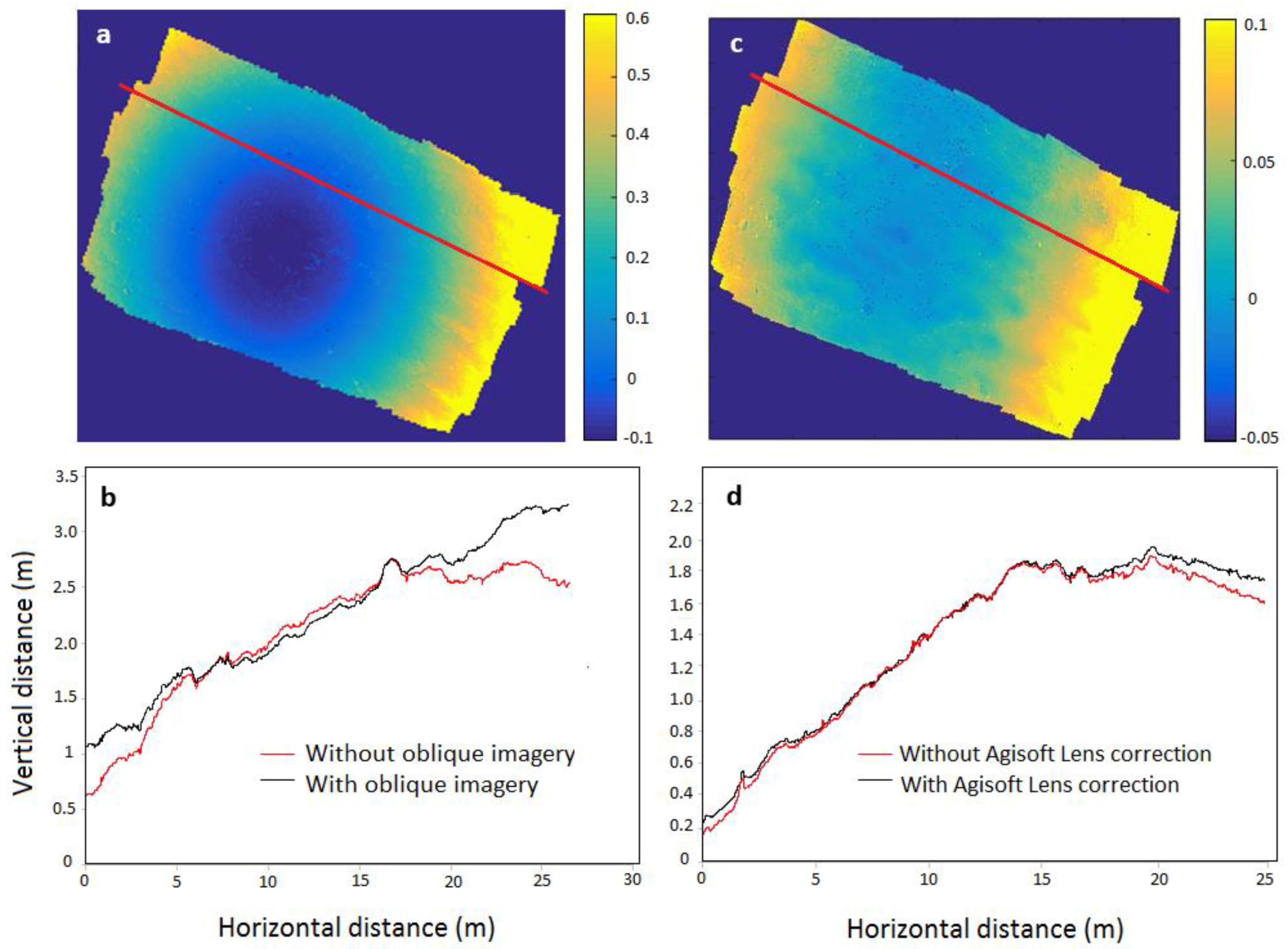
• Radial lens distortion correction. The geometry of the camera lens accounts for some degree of distortion in the images [36,40]. Radial distortion particularly affects the geometry of the image and is accentuated as the focal length is reduced, thereafter having a direct impact in SfM reconstructions and generating non-linear deformations in the 3D models if the FOV angle is wide [40]. Recent studies show that systematic errors in topographic models derived from UAS-borne SfM surveys might arise in the photogrammetric reconstruction due to a combination of the near-parallel imaging collection pathways taken in traditional UAS mapping surveys, and an inaccurate correction of radial lens distortion [33]. A solution to this issue was investigated by testing two different approaches; the use of the freely available Agisoft Lens and the addition ‘striped’ oblique imagery over a small snow-covered surface generated from an imagery sub-set.

The combination of these two pre-processing techniques was thoroughly tested for fifty image subsets comprising diverse types of snow surface type, illumination, camera type and image quality. For each test, the comparison between pre-processed and non-processed was made using the same Agisoft Photoscan Pro settings which were chosen depending on the photoset characteristics. The improvement was measured by observing the number of matches between image pairs, the number of sparse and dense point clouds density and changes in the number points selected with the projection error tool of Photoscan [35]. A range of different model building qualities were also tested. This process downscales the source images by a defined number of times on each side from low (to 12.5%) to high (no downscaling). These values were carefully evaluated considering the noise generated by clouds in the visual observations at both small (cm) and large (m) scale. Following the positive testing outcomes, both procedures were applied to all photosets. Details of such tests plus considerations for the image pre-processing workflow, including the effect of conserving high bit depth imagery by converting the RAW data to TIFF (12 bit) relative to the JPEG format (8 bit), can be found in Appendix C.

3.4.2. GNSS Post-Processing of GCP Data

The GNSS data of the GCPs was post-processed using the differential GNSS method [41]. The Svalbard Satellite Station (SvalSat) was used as the baseline for the Svalbard areas which were located approximately 5 km from the studied areas (78°13′45.9″N 15°23′42.9″E, WGS 84). For Greenland, the Sisimiut reference station, located approximately 29 km from the studied areas (66°56′06.8″N 53°38′37.8″W, WGS 84) was used as a baseline. The agencies in charge of the reference stations (Kongsberg Satellite Services and DTU Space) provided the precise location of their reference stations and the 24 h positioning data acquired for each of the surveyed days. The reference station data was accessed using the Hatanaka compression and decompression program, providing the RINEX files (data interchange format for raw satellite navigation system data). The GNSS data downloaded from the JAVAD receivers were also transformed to RINEX using jps2rin open-source software. The corrections were computed through the Leica Geo Office (LGO) software. As provided by LGO, the static GNSS method with post-processed differential corrections achieved an average position and height better than 0.02 m depending on the area and survey region.

3.4.3. SDEMs and TDEMs Generation in Agisoft Photoscan Pro

Images in Photoscan can be aligned at low, medium, or high accuracy depending on the scale of features of interest to be reconstructed [35]. The selection of alignment accuracy depended on snow surface type, photoset image quality and required processing time. For low-quality images (characteristic of low light conditions and from the minimal set-up) and for smooth snow areas, medium accuracy is preferred due to the paucity of small-scale features to match and because reconstruction might be confounded by the associated digital noise. With better image quality from the advanced set-up, a high reconstruction quality is preferable. However, we found this to be redundant considering the small GSD of 0.001–0.004 m pixel⁻¹ obtained and with low reconstruction quality still providing centimeter-scale GSD in the downscaled images. A high reconstruction quality is preferred for the summer areas to compensate for the poor camera positions of the land-based surveys.

The processing time was noticeably reduced by the image pair preselection option (generic), which pre-matched image pairs with reduced matching constraints. The sparse clouds generated from the alignments were manually edited and filtered with Photoscan Pro built-in tools for removing evident outliers (cloud points detached from the overall reconstructed surface) and noise in the point clouds. The sparse clouds were georeferenced by manually identifying the GCP in the matched pictures and assigning them the coordinates from the GNSS post-processing. At this stage, also the natural CGCPs available and further identified (mainly common identifiable rocks), were used to co-georeference the winter and summer DEMs. Co-georeferencing consists of georeferencing both snow and terrain DEMs with common visible features of known precise location with the purpose of mitigating errors in the final snow depth estimation. These common recognizable points had been directly measured with the GNSS station at the ground level. The number of GCPs, and common GCPs (CGCPs) used for both the summer and winter DEMs are listed in Table 1.

For the dense cloud reconstruction process, all areas were reconstructed at a low or medium reconstruction quality in Photoscan Pro because of the high computational costs. The reconstruction quality selection criteria were the same for the sparse reconstruction. Photoscan reconstruction quality affects the source imagery resolution by downsampling. For low, resolution is reduced eight times (to 12.5%) on each side reducing the imagery GSD. However, due to the millimeter GSDs photoset quality (Table 2), the image resolution still resulted in very detailed and accurate centimeter order geometry. Triangular meshes of the areas were finally generated from the dense clouds with a high polygon count using the standard proposed triangulation in Photoscan Pro and without any interpolation method.

3.4.4. Snow Depth Retrieval

For each of the studied areas, snow depth was derived by subtracting the underlying topography TDEM from the snow surface SDEM. The final square size of the output raster grid is made equal for both DEMs by choosing the lower resolution DEM (usually the terrain DEM due to the land-based surveys) as reference.

3.4.5. Error Analysis and Quality Assessment of the Snow Depth Maps

The produced DEMs are subject to two types of error: (i) a photogrammetric reconstruction error which depends on the overall quality of the photosets, and (ii) a georeferencing error influenced by the GNSS post-processing quality, the GCPs allocation and identification in the images, and the antenna height measurements.

The quality of the photogrammetric 3D reconstruction was assessed based on the point cloud density and the output resolution of the DEMs, which are directly linked with the number of points that the SfM algorithm could match and thus indicates how well a surface was reconstructed. Attention was paid to visually inspecting the point cloud noise and to the correct representation of snow surface cover at both small (e.g., reconstruction of sastrugi and snow ripples) and large scales (e.g., holes in the DEM and snow drift accumulation areas) by comparison with in situ imagery. The quality of each reconstructed 3D model is also assessed individually by using an indicator of the reconstruction uncertainty such as the difference between the reconstructed and measured position at the GCPs. This is quantified as the RMSE of the Euclidean distance between the reference coordinates of the GCPs to the corresponding estimated points in the reconstructed 3D model (provided by Photoscan).

It is challenging to break down each component influencing the georeferencing error. However, the error of the GNSS post-processing is considered to be on the same order of magnitude as the GSD after the images were downsampled, and as the uncertainty inherent to the GCPs identification on the images. As snow depth is derived by subtracting the SDEM from the TDEM, the total error is the sum of both SDEM and TDEM error. The most straightforward validation approach is based on a comparison with the probed snow depths at the SDEMs GCP positions and at the few additional samples taken post survey (for Sval2 and Green4). These points will be termed validation points (VPs). We can then analyze the mean bias, RMSE and error distribution for these areas to provide an estimate of the uncertainty on the snow depth product over these points. As validation is biased around GCP positions [32], an additional validation is performed by comparing corresponding pixels of snow-free areas away from the GCP positions. Assuming no change in the terrain between the winter and summer campaign, the snow depth should equal zero for these areas. The snow-free areas are automatically selected as cells with a mean RGB value lower than 0.2 in the RGB orthomosaics. This simple threshold was chosen to be very conservative based on visual inspection of the snow-free areas for each orthomosaic. While with this threshold not all snow-free pixels are detected, it guarantees that shadowed (dark) snow pixels are not incorrectly selected as snow-free. This was visually verified.

4. Results

Here we present the TDEMs, SDEMs, and final snow depth retrieval for our surveys. Detailed results pertaining to the snow imagery pre-processing described in the materials and methods section are provided in Appendix C.

4.1. SDEMs and TDEMs Reconstruction

A total of 11 DEMs were generated from the winter and summer fieldwork campaigns. The total error, point cloud densities, output resolution, and other mapping parameters for each DEM are summarized in

Table 3. Summary of the Photoscan reconstruction quality and details of analysis for all survey areas. Shown is the ground sample distance (GSD) for the acquired imagery and the final resolution of the Digital Elevation Models (DEMs). The total error represents the Root Mean Square Error (RMSE) of the Euclidean distance from the reference GCPs to the corresponding points estimated in the 3D model. SDEM and TDEM refer to snow and terrain, respectively.

Area Name	GSD (m pixel−1)		Photoscan Reconstruction Quality (Dense)		Points Cloud Density (Points m−2)		DEMs Final Resolution (m)		Total Error (RMSE) (m)
	SDEM	TDEM	SDEM	TDEM	SDEM	TDEM	SDEM	TDEM	SDEM	TDEM
Sval1	0.003	0.003	Medium	Medium	1337.5	273.6	0.03	0.06	0.09	0.057
Sval2	0.004	0.003	Medium	Medium	801.5	301.1	0.04	0.09	0.044	0.054
Green1	0.003	0.009	Medium	High	1518.5	163.7	0.04	0.1	0.057	0.23
Green2	0.001	0.006	Low	High	4284.5	80.0	0.02	0.09	0.045	0.093
Green3	0.003	0.021	Low	High	4413.1	133.2	0.02	0.09	0.05	0.086
Green4	0.004		Low	High	3867.8		0.03	0.09	0.04

.

Overall, with ad hoc image acquisition and image pre-processing, the SfM methodology was able to reconstruct different snow surfaces for both high and low light days and with different UAS/sensor systems. In all cases, centimeter-scale mapping was achieved (Table 3). For the Greenland sites, land-based surveyed TDEM depicts a lower quality than the UAS-based winter SDEM due to the limited points of view from which the survey could be performed. Nonetheless, it still achieved decimeter resolution (Table 3).

Both light availability and snow surface type were found to play a role in the reconstruction quality. For example, without pre-processing, the minimal set-up was unable to map smooth areas and produced relatively rough point clouds compared to the smooth nature of that snow type (Appendix C). A decrease in point cloud densities was also observed for areas mapped with the advanced set-up as light availability decreased (Table 3). Lower achieved resolutions and reconstructions were observed for the SDEMs derived from the minimal set-up compared to the advanced set-up (Table 3). This is attributed to the less favorable conditions of smooth snow/overcast sky (Table 1) and the inferior quality of the sensor (extra noise), which required an inferior image quality reconstruction setting.

The total error for the land-based SfM was higher compared to the UAS mapped areas due to the limited number of available camera positions (shown in Figure 2), which affected the geometry reconstruction and the GCP identification in the images. Accordingly, the point cloud densities were also affected by the inferior quality of these surveys.

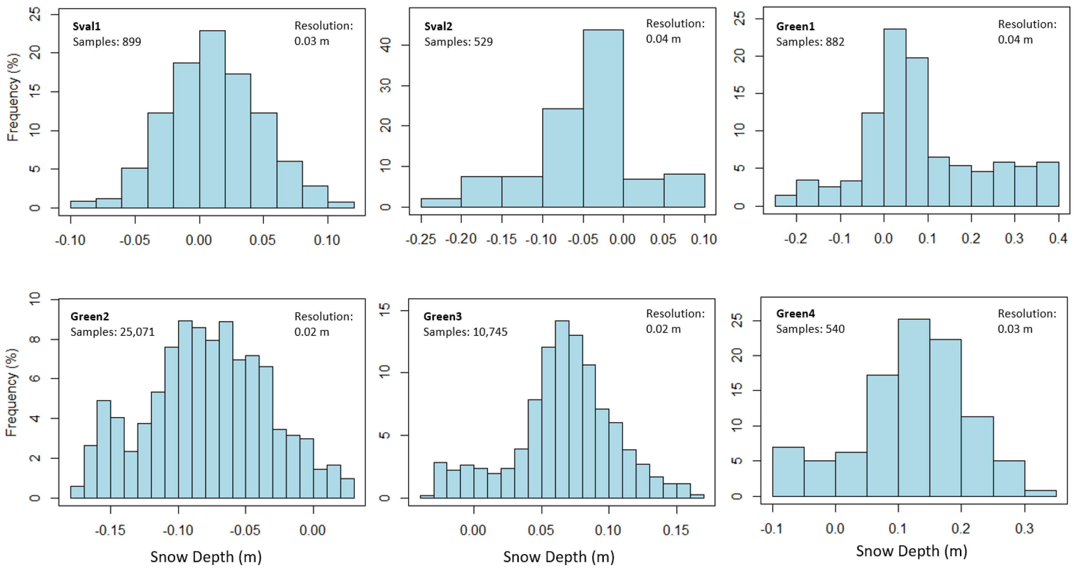
4.2. Snow Depth Retrieval

Snow depth maps produced for each of the studied areas are presented in Figure 4 along with the difference between probed (HS_m) and estimated snow depth (HS_UAS) at the VPs locations. The mapping resolutions achieved together with the snow depth validation statistics are presented in

Table 4. Summary of the results corresponding to the estimated snow depth maps for all the different surveyed areas. Average difference between the measured snow depth HS_m and the estimated snow depth HS_UAS is calculated for the validation points (VPs). The standard deviation is in regards of the average difference between the VPs. RMSE refers to Root Mean Square Error between measured and estimated snow depth.

Area Name	Area Covered (m2)	Snow Depth Map Resolution (m)	VPs	Average Difference $\mathit{H}{\mathit{S}}_{\mathit{m}}-\mathit{H}{\mathit{S}}_{\mathit{U}\mathit{A}\mathit{S}}$ (m)	Standard Deviation (m)	RMSE $\mathit{H}{\mathit{S}}_{\mathit{m}}-\mathit{H}{\mathit{S}}_{\mathit{U}\mathit{A}\mathit{S}}$ (m)
Sval1	6100	0.06	8	0.0379	0.0457	0.0594
Sval2	1386	0.09	5	0.0156	0.0428	0.0456
Green1	2738	0.1	4	0.0873	0.0985	0.1317
Green2	2260	0.09	11	0.161	0.0928	0.1857
Green3	38,410	0.09	9	0.038	0.0862	0.0943
Green4	27,687	0.09	7	0.021	0.086	0.0887

. Validation statistics include the average difference (or mean bias) and the RMSE between HS_m and HS_UAS. The results indicate an overall good performance for all the surveyed areas with results agreeing with relevant literature [27]. These results confirm the overall feasibility of the proposed low-cost method capture snow depth variability over different types of snow covers in the Arctic as compared to traditional methodologies.

The outcomes of the additional validation method using snow free areas are shown in Figure 5 as distribution histograms. The HS_UAS estimates are expected to be mostly distributed around the zero values over the tracked dark pixels (normal distribution). Although not overly representative of the snow-covered areas, this test assists on quantifying the performance of the method further away from the GCPs and exposes the nature of the DEM bias (translated, rotated, or deformed) through comparison with the underlying topography. The sample size for each snow-free validation point corresponds to the snow surface DEM resolution for that area (Table 3). The number of samples for each study area is dependent on the resolution of the orthophoto, the number of snow-free areas, and orthophoto contrast characteristics.

Centimeter-scale average difference was achieved at the VPs at Sval1 and Sval2 (Table 4). The snow-free validation is in agreement with these observations for both areas with an evident normal distribution (Figure 5). The snow-free control areas are positively characterized by a well-distributed network (Figure 1). Greenland areas provided centimeter to decimeter average difference and RMSE in the VPs (Table 4). However, the average difference increased slightly in comparison to the Svalbard areas. This is attributed to the land-based surveys of the underlying topography, which provided coarser and less accurate TDEMs for snow depth calculation. The snow-free VPs distributions for areas Green1, Green3 and Green4 (Figure 5) also presented a normal distribution centered near zero, although a skewed histogram is clearly observed with a slight HS_UAS overestimation. This was attributed in part to the wrong surface interpolation around boulders edges surrounded by snow (example in Figure 2e).

Vegetation cover was usually present in areas where an underestimation of HS_UAS was observed (slightly negative, blue values in Figure 4). Green1, Green3, and Green4 presented zones associated with negative HS_UAS, which coincide with the rise of grass vegetation. This resulted in an underestimation of approximately the observed grass height (5–15 cm). For area Green2, control trough VPs resulted particularly affected around areas with thick vegetation such as the slope. This is observable by comparing its error map (Figure 4) and the visible vegetation in Figure 1 orthomosaic and in Figure 2f. It is plausible that this led to the considerable underestimation of the HS_UAS for these points. This possibility is also suggested by the Green2 snow-free validation histogram in Figure 5 that displays a clear bias towards negative HS_UAS. It is also suspected that the lack of co-georeferencing for this area could have affected the results.

Difference between the individual DEMs total errors (Table 3) and the snow depth validation statistics (Table 4) confirms that the co-georeferencing plays an important role in mitigating the error on the estimated HS_UAS by rendering the DEMs subtraction relative to their own reference system.

5. Discussion

5.1. Effect of Snow Surface Type, Light Conditions, and Image Quality

Two limitations are known to affect SfM performance in a geoscience context, non-linear deformations and image texture dependence [20,21]. In our study, we countered the issue of non-linear deformation by ensuring accurate visual observations of the reconstructed snow surfaces, a targeted geometric image pre-processing and the implementation of the Photoscan built-in function optimization, which performed well with the accurate GCPs collected for this study [35]. In this work, we are primarily investigating the latter SfM caveat in relation to featureless surfaces, such as snow, that can be further affected by poor lighting conditions.

Snow surface reconstruction was demonstrated to be successful for all tested cases employing two opposite extremes of imaging quality, the minimal and advanced set-up. We found image acquisition was critical because SfM performance relies heavily on the quality of the image (Appendix B and Appendix C), especially when the subject lacks natural features for reconstruction or when contrast inducing luminance is lacking [23,24]. It is also optimal for the camera’s internal parameters (focal length, aperture, ISO, and shutter speed) to be set according to the camera’s capabilities, the snow surface type, and the actual luminance conditions depending on the aimed resolution (or GSD) and the UAS flying parameters (altitude and speed) (see Appendix B for more information).

Nevertheless, both luminance and snow surface type were observed to have an impact in the SfM reconstruction of snow surfaces. The effect of luminance availability, as observed in the SDEM production (Table 3 and visual observations), was found to be more influential than the snow surface type for both camera set-ups. This is attributed not only to the lack of contrast and features in the images but also to the fact that, in combination with the faster shutter-speeds required for a moving platform, it can produce dark images characterized by increased noise, leading to incorrect surface interpolations or a complete lack of matched points (Appendix C). This was evident for the inferior optical performance of the minimal set-up.

We can treat the minimal set-up as the “worst-case” scenario from a SfM and available equipment perspective. With the proposed image pre-processing, the set-up was nevertheless able to provide results in overcast conditions and/or over featureless snow. Such set-ups are extremely low-cost, lightweight, and easy to use. They are also capable of acquiring images in a dynamic manner characteristic of small action cameras. These are very useful assets for small surveys in remote Arctic areas where carrying volume, weight, and overall logistics are constraints. In addition, their low weight reduces regulation concerns (Appendix A). However, their inferior sensor size and fore-optics are limiting, requiring a lower altitude flight to achieve the same resolution as the advanced set-ups, and thus are not suited for mapping larger areas. They also involve a higher degree of digital noise, which in certain circumstances affects the fine-scale quality of the reconstructions and the application of the image pre-processing workflow (Appendix C).

The advanced set-up is capable of flying at higher altitudes and mapping larger areas with improved cameras that provide better mapping outcomes through the photogrammetric formulas (Appendix B). However, one disadvantage is that the advanced set-up camera parameters need to be manually set accordingly to the survey circumstances (Appendix B). They are also considerably heavier, have reduced flight time, are more challenging to operate, and are subject to more regulations.

The effect of the image pre-processing workflow was not as critical to the advanced set-up as for the minimal set-up (Appendix C). However, the extra matched points have an impact on the resolution of the final SDEM produced. The number of matching points is directly linked to point cloud densities and thus affects the spatial resolution of the DEMs and consequently the estimated snow depth. The spatial resolution might affect the uncertainty of the volume estimations, especially for complex underlying topographies where the snow depth can significantly vary at the micro-scale level. The spatial resolution results are even more important in a snow-sampling context, as observed in some other studies [19,42].

To achieve high-quality reconstruction quality, it is important that the UAS set-up (image quality) and flying parameters are optimized for the required areal coverage, the snow surface type and light conditions. In addition, the scale of features of interest that assists the surface reconstruction (e.g., sastrugi, ripples, and relief) should be higher than the expected digital noise. Otherwise, it will decrease the number of proper matches and produce noisy surfaces. As shown in the image pre-processing results (Appendix C), it is important to find a balance between the pre-processing enhancement intensity and Photoscan’s reconstruction quality, so that the effect of noise is minimized compared to the scale of the matched features.

Future work is needed to investigate the further advantages of using RAW imagery by testing different sharpening and content enhancement approaches or the use of infrared photography to enhance snow features, as explored in other studies [26,43].

Although various surveying conditions were investigated in this study, extreme cases such as long-lasting polar nights experienced in higher-latitude Arctic locations might impede this methodology due to a lack of luminance. The period after the snow peak season is of great interest, since its characterized by increased snow depth variability that continues through the subsequent melting season [11]. Nevertheless, low luminance winter measurements are increasingly required [1] and should be considered for future work.

It is important to note that these conceptual tests were performed over relatively small areas (1386 to 38,410 m²) and flying at relatively low altitudes above ground (7 to 26 m), thus achieving very high GSDs (0.001 to 0.004 m pixel⁻¹). However, the retrieved images were downscaled (between four to eight times) during the cloud reconstruction process. Theoretically, this suggests that using the same settings of the advanced set-up, for example, the flying altitude can be set to 150 m and achieve the same mapping parameters. Such a setting would allow a photographic footprint of 24,704 m² and still provide a GSD of 0.03 m pixel⁻¹ based on normal photogrammetric formulas (Appendix B). Nevertheless, the drop in elevation accuracy associated with flying at higher altitudes needs to be considered and evaluated. The scalability of the proposed method would be an interesting aspect to consider for future studies as well.

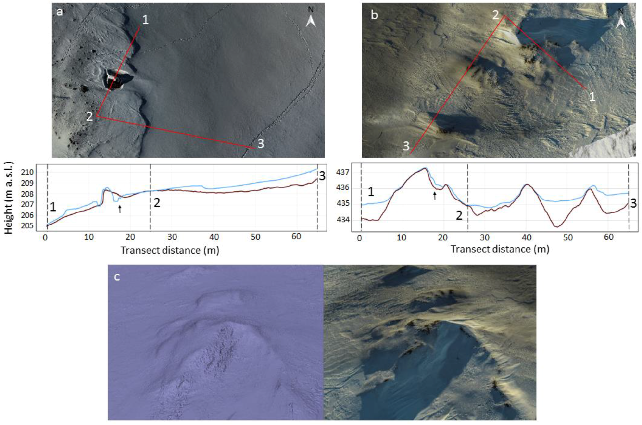
5.2. Effect of Underlying Topography

Overall, snow depth variability was successfully captured over a range of simple, steep, and complex underlying topographies, and a combination of SfM approaches (land- and UAS-based). For small-scale areas, high-resolution estimates are needed when monitoring complex and highly variable underlying topographies, as shown in Figure 6. This is relevant in the Arctic as snow drift accumulation and sastrugi features are common and require improved resolutions for capturing their variability. In the produced snow depth maps, a high level of resolution can be seen in the capture of sastrugi features, footsteps, and leeside snow drift accumulation areas within SDEMs transects (Figure 6).

Some errors arose in the land-based surveys due to the poor camera positions compared to an UAS survey (Figure 6). Shadowed areas caused by a low sun angle and terrain relief also downgraded the reconstruction performance in terms of point cloud noise (Figure 6c). In this context, it was also noticed how any unnatural features such as footsteps conversely assisted the reconstruction of these feature-less areas (not shown). Although the number of VP samples was very low, different slope inclinations correspondingly showed increased drift accumulation. These did not display any particular increase in error in relation to whether the VPs were located in steep or moderate slope areas (Figure 4).

Surveys in the Arctic are characterized by a low solar zenith angle that creates positive shadows (patterns) for most surface irregularities. A recommendation for future surveys would be to collect the observations at the local solar noon. This would limit the noise generated by large-scale topography-induced shadows (Figure 6c), but maintain shadowing of small snow features (e.g., snow ripples), which generates contrasting patterns that aid in the reconstruction process.

As previously discussed, a major limitation in relation to underlying topography arose from the vegetation cover, as shown for the Greenland areas. This was because of the inability of SfM to reconstruct the topography beneath the vegetation, resulting in a reconstructed surface above the height of the vegetation. Combining SfM with laser scanning has proven successful in mapping absolute terrain heights for low canopy closures [44], but as in this and previous studies, thick bushes still remain a problem [26]. One solution would be to survey the summertime terrain DEM with LiDAR systems and then repeatedly use the UAS-SfM method for the winter DEMs. The terrain DEM could then be reused in subsequent years if the underlying topography does not change in a significant way. Another option would be to classify the terrain orthophotos based on vegetation type and subtract average vegetation heights, even though additional error would arise due to the potential variability in vegetation heights.

Land-based SfM can be used as an alternative when technical issues with UAS deployments are experienced, if suitable vantage points are available. However, it is considerably more labor-intensive and time-consuming, and ultimately the SfM reconstruction results are compromised due to the sub-optimal image perspective when compared to orthogonal imagery [35]. An additional drawback of land-based SfM is its inability to capture information behind obstructing features (e.g., boulders) due to poor interpolation, as seen in area Green1, resulting in erroneous snow depth estimates (Figure 6).

5.3. The Niche Role of Low-Cost UAS Platforms for Snow Depth Mapping in the Arctic

The proposed snow mapping method is applicable for all the surveyed scenarios with the tested equipment. The average difference between measured and estimated snow depth ranged between 0.015 m and 0.16 m, with the RMSE between 0.05 to 0.18 m. Although these statistics are based on a limited validation power (see validation caveats section), these values are comparable to LiDAR estimates, with reported RMSE of single DEMs as great as 0.1 m and accuracies of snow depth estimates of 0.15 m [21]. The spatial resolutions for our method ranged from 0.06 to 0.09 m, whereas for LiDAR airborne datasets are on the order of 1 m point spacing [21].

While the technical set-ups investigated in this study are theoretically capable of mapping considerably larger areal extents, this method is, however, not intended as a substitute for airborne LiDAR, which will always be more efficient at covering catchment-scale areas. This low-cost UAS method is instead intended as an easily applicable economic alternative to track snow depth in relatively small areas that require high spatial resolution and ease of repeatability.

This low-cost and high-resolution methodology for mapping snow depth is applicable to many research and civil applications in the vast and sparsely populated Arctic, where observing power is limited [1]. Minimal set-ups (e.g., DJI Phantom^® UASs and GoPro^®) are nowadays extremely common and affordable. Beyond Arctic researchers requiring snow depth estimates across multiple disciplines, the demonstrated workflow can also assist local environmental and municipal entities. This use of consumer-grade equipment for scientific applications is also beneficial in terms of the cost, ease of handling, and ability to perform in extreme conditions. Other opportunities are also foreseen through engagement in citizen science as individual use of these easily affordable solutions grows [40,45].

5.4. GCPs Limitation and Co-Georeferencing

A limitation of our method is the time and manpower required to use GCPs for georeferencing the reconstructed 3D models. In addition, our survey sites benefitted from the availability of nearby reference stations whose presence is not guaranteed in the majority of remote Arctic locations. Nevertheless, other positioning techniques could be employed such as real-time kinematic (RTK) surveys with a local master station, for example. RTK is swifter compared to static GNSS surveys, and the rapid advancement of the technology is achieving comparable accuracies with less effort involved.

Another interesting option is the use of on-board dual frequency GNSS receivers on the UAS sensor load that are capable of providing sensor position and orientation for each frame for direct sensor orientation (DSO) [46,47,48]. In DSO, the exterior orientation parameters for each image are computed by processing the on-board GNSS and the Inertial Measurement Unit (IMU) data, thus bypassing the deployment and acquisition of GCPs. Such techniques are not yet capable of providing the same accuracy as GNSS positioning in static, ground-based surveys (centimeter to millimeter scale), but it is expected that these technological challenges will be surpassed in the future and GCPs will not be required anymore.

Finally, our results confirm that co-georeferencing can provide improved snow depth estimates. Consequently, common visible points can be acquired only once and then repeatedly used for georeferencing the time-variable snow surfaces. GCP surveys would only need to be performed once for the area of interest. These points could be natural features or artificially placed markers (e.g., poles that stand above the snow surface) with precisely known positions distributed around the monitored area of interest.

5.5. Validation Caveats

The validation applied in this study is limited by (i) the relatively low number of VPs (a total of 31 snow probed GCPs and samples on the SDEMs comprising a total cumulative area of 78,581 m²) and (ii) the fact that the accuracy has a biased improvement around the position of the GCPs. On the other hand, the produced DEMs gain reliability if the GCP network is dense and properly distributed, with the GCPs’ areal coverage being more important than the actual number of GCPs [32]. In our case, GCPs for most of the areas are relatively well distributed. Additionally, the snow-free validation provided extra information (Figure 5) on multiple points that were distant from the GCPs, as can be seen from the areas’ orthomosaics (Figure 1). Even though these are not representative for snow-covered areas, they indicate a coherent SDEM reconstruction in terms of rotation, translation, and deformation of the generated model relative to the true topography.

Many studies have used several markers as GCPs or other features spread around the snow surface, e.g., poles and crosses, to manually measure snow depth [15]. Our study comprised a reduced number of displaced GCPs markers in comparison to other studies that employed a very dense validation network grid (e.g., [18]). It is suspected that such a grid and its allocation process in our case would have greatly assisted the SfM reconstruction by disturbance of the snow surface, as shown by [23]. One of our aims was to leave the snow surface undisturbed to test the known SfM limitations relating to the absence of texture and features.

Although the use of fast-static or RTK survey techniques post UAS-survey could have provided the desired positioning accuracy given the scale of the spatial resolution achieved, the allocation of a large number of features would have compromised the snow surface.

While this study does not claim to provide a full accuracy evaluation for the method, it demonstrates its capability to capture complex snow depth variability for a set of previously unexplored survey conditions, using extremely low-cost solutions and in a logistically challenging environment. Notwithstanding, uncertainties remain and further validation methods should be tested by comparison with other spatially significant methods such as LiDAR (e.g., [49]) or the addition of non-invasive extra control points. The effect of increased flying altitudes on the performance of the proposed method should also be investigated.

6. Conclusions

Estimating snow depth distribution for small-scale areal extents in Arctic regions is of great importance for many applications ranging from scientific research to civil purposes.

This study showcased a low-cost solution employing commonly available UASs and camera payloads to produce snow depth maps at high resolution for a variety of surveying conditions. The method was tested using two different UAS/payloads systems ranging from a minimal set-up (~500 USD employing a GoPro^® Action camera) to a more complex and advanced solution (~1700 USD employing a DSLR camera) (Table 2). While the set-ups differed in terms of ease of use, cost, and image quality, the photogrammetric considerations were similar.

Six areas were mapped, two in Svalbard and four in Greenland, covering areal extents from 1386 to 38,410 m². Overall, through appropriate image pre-processing approaches, DEMs for varying, snow surfaces types (from smooth to sastrugi sculpted snow), mapped under different light conditions (from overcast to clear sky), could be properly reconstructed using both UAS systems even for the worst case scenario (overcast sky with the minimal set-up). Although not considered a comprehensive evaluation of accuracy, the average difference between UAS-estimated and measured snow depth, checked with conventional snow probing, ranged from 0.015 to 0.16 m.

The resolutions of the snow depth maps ranged from 0.06 m to 0.01 m (Table 4) and were mostly limited by the inferior performance of the land-based surveys performed for some of the mapped snow underlying topographies. Based on theoretical photogrammetry formulas, the resolution can be further optimized depending on the desired output and equipment available to map greater areal extents, although inaccuracies associated with flying at higher altitudes would need to be evaluated. This study demonstrated the potential to overcome SfM limitations relating to featureless surfaces such as snow through the application of image pre-processing workflows and a proper image acquisition phase, which are ideally tuned for each specific circumstance. Image noise and the scale of the recognizable image features are key parameters to be considered when applying histogram stretching pre-processing techniques.

The deployment of UASs in the Arctic is rapidly expanding due to the wide range of applications it offers for environmental and earth science research. Surveying polar environments is logistically challenging, requiring an extra degree of flexibility and ease of deployment when surveying highly variable surfaces like snow. The successful workflow outlined in this study provides important guidance for designing future surveys, with the specific direction dependent on desired outcome, available budget, and surveying conditions.

References

1. Bokhorst, S.; Pedersen, S.H.; Brucker, L.; Anisimov, O.; Bjerke, J.W.; Brown, R.D.; Ehrich, D.; Essery, R.L.H.; Heilig, A.; Ingvander, S.; et al. Changing Arctic snow cover: A review of recent developments and assessment of future needs for observations, modelling, and impacts. Ambio 2016, 45, 516–537. [Google Scholar] [CrossRef] [PubMed] [Green Version]
2. Callaghan, T.V.; Johansson, M.; Brown, R.D.; Groisman, P.Y.; Labba, N.; Radionov, V.; Bradley, R.S.; Blangy, S.; Bulygina, O.N.; Christensen, T.R.; et al. Multiple Effects of Changes in Arctic Snow Cover. Ambio 2011, 40, 32–45. [Google Scholar] [CrossRef]
3. Morgner, E.; Elberling, B.; Strebel, D.; Cooper, E.J. The importance of winter in annual ecosystem respiration in the High Arctic: Effects of snow depth in two vegetation types. Polar Res. 2010, 29, 58–74. [Google Scholar] [CrossRef]
4. Wipf, S.; Stoeckli, V.; Bebi, P. Winter climate change in alpine tundra: Plant responses to changes in snow depth and snowmelt timing. Clim. Chang. 2009, 94, 105–121. [Google Scholar] [CrossRef]
5. Gisnås, K.; Westermann, S.; Schuler, T.V.; Litherland, T.; Isaksen, K.; Boike, J.; Etzelmüller, B. A statistical approach to represent small-scale variability of permafrost temperatures due to snow cover. Cryosphere 2014, 8, 2063–2074. [Google Scholar] [CrossRef]
6. Slater, A.G.; Lawrence, D.M. Diagnosing Present and Future Permafrost from Climate Models. J. Clim. 2013, 26, 5608–5623. [Google Scholar] [CrossRef]
7. Campbell, K.; Mundy, C.J.; Barber, D.G.; Gosselin, M. Characterizing the sea ice algae chlorophyll a–snow depth relationship over Arctic spring melt using transmitted irradiance. J. Mar. Syst. 2015, 147, 76–84. [Google Scholar] [CrossRef]
8. Haapala, J.; Lensu, M.; Dumont, M.; Renner, A.H.H.; Granskog, M.A.; Gerland, S. Small-scale horizontal variability of snow, sea-ice thickness and freeboard in the first-year ice region north of Svalbard. Ann. Glaciol. 2013, 54, 261–266. [Google Scholar] [CrossRef]
9. Alavedra, J.M.I.; Iglesias, J.P.; López, J.T.; Figueras, P.M.I.; Baños, I.M.; Figueras, P.O.I.; García, A.R. Assessment of airborne LIDAR for snowpack depth modeling. Bol. Soc. Geol. Mex. 2011, 63, 95–107. [Google Scholar]
10. Grünewald, T.; Stötter, J.; Pomeroy, J.W.; Dadic, R.; Moreno Baños, I.; Marturià, J.; Spross, M.; Hopkinson, C.; Burlando, P.; Lehning, M. Statistical modelling of the snow depth distribution in open alpine terrain. Hydrol. Earth Syst. Sci. 2013, 17, 3005–3021. [Google Scholar] [CrossRef]
11. López-Moreno, J.I.; Revuelto, J.; Fassnacht, S.R.; Azorín-Molina, C.; Vicente-Serrano, S.M.; Morán-Tejeda, E.; Sexstone, G.A. Snowpack variability across various spatio-temporal resolutions. Hydrol. Process. 2014, 29, 1213–1224. [Google Scholar] [CrossRef]
12. Barnett, T.P.; Adam, J.C.; Lettenmaier, D.P. Potential impacts of a warming climate on water availability in snow-dominated regions. Nature 2005, 438, 303–309. [Google Scholar] [CrossRef] [PubMed]
13. Schweizer, J.; Kronholm, K.; Jamieson, J.B.; Birkeland, K.W. Review of spatial variability of snowpack properties and its importance for avalanche formation. Cold Reg. Sci. Technol. 2008, 51, 253–272. [Google Scholar] [CrossRef]
14. Tominaga, Y.; Okaze, T.; Mochida, A. CFD modeling of snowdrift around a building: An overview of models and evaluation of a new approach. Build. Environ. 2011, 46, 899–910. [Google Scholar] [CrossRef]
15. Scipión, D.E.; Mott, R.; Lehning, M.; Schneebeli, M.; Berne, A. Seasonal small-scale spatial variability in alpine snowfall and snow accumulation. Water Resour. Res. 2013, 49, 1446–1457. [Google Scholar] [CrossRef]
16. Callaghan, T.V.; Johansson, M.; Brown, R.D.; Groisman, P.Y.; Labba, N.; Radionov, V.; Barry, R.G.; Bulygina, O.N.; Essery, R.L.H.; Frolov, D.M.; et al. The Changing Face of Arctic Snow Cover: A Synthesis of Observed and Projected Changes. Ambio 2011, 40, 17–31. [Google Scholar] [CrossRef]
17. Melvold, K.; Skaugen, T. Multiscale spatial variability of lidar-derived and modeled snow depth on Hardangervidda, Norway. Ann. Glaciol. 2013, 54, 273–281. [Google Scholar] [CrossRef]
18. Prokop, A.; Schirmer, M.; Rub, M.; Lehning, M.; Stocker, M. A comparison of measurement methods: Terrestrial laser scanning, tachymetry and snow probing for the determination of the spatial snow-depth distribution on slopes. Ann. Glaciol. 2008, 49, 210–216. [Google Scholar] [CrossRef]
19. Liston, G.E.; Sturm, M. Winter Precipitation Patterns in Arctic Alaska Determined from a Blowing-Snow Model and Snow-Depth Observations. J. Hydrometeorol. 2002, 3, 646–659. [Google Scholar] [CrossRef]
20. Slater, A.G.; Clark, M.P. Snow Data Assimilation via an Ensemble Kalman Filter. J. Hydrometeorol. 2006, 7, 478–493. [Google Scholar] [CrossRef]
21. Deems, J.S.; Painter, T.H.; Finnegan, D.C. Lidar measurement of snow depth: A review. J. Glaciol. 2013, 59, 467–479. [Google Scholar] [CrossRef]
22. Smith, M.W.; Carrivick, J.L.; Quincey, D.J. Structure from motion photogrammetry in physical geography. Prog. Phys. Geogr. 2015, 40, 247–275. [Google Scholar] [CrossRef]
23. Westoby, M.J.; Brasington, J.; Glasser, N.F.; Hambrey, M.J.; Reynolds, J.M. “Structure-from-Motion” photogrammetry: A low-cost, effective tool for geoscience applications. Geomorphology 2012, 179, 300–314. [Google Scholar] [CrossRef] [Green Version]
24. Fonstad, M.A.; Dietrich, J.T.; Courville, B.C.; Jensen, J.L.; Carbonneau, P.E. Topographic structure from motion: A new development in photogrammetric measurement. Earth Surf. Process. Landf. 2013, 38, 421–430. [Google Scholar] [CrossRef]
25. Ryan, J.C.; Hubbard, A.L.; Box, J.E.; Todd, J.; Christoffersen, P.; Carr, J.R.; Holt, T.O.; Snooke, N. UAV photogrammetry and structure from motion to assess calving dynamics at Store Glacier, a large outlet draining the Greenland ice sheet. Cryosphere 2015, 9, 1–11. [Google Scholar] [CrossRef]
26. Bühler, Y.; Adams, M.S.; Bösch, R.; Stoffel, A. Mapping snow depth in alpine terrain with unmanned aerial systems (UAS): Potential and limitations. Cryosphere 2016, 10, 1075–1088. [Google Scholar] [CrossRef]
27. De Michele, C.; Avanzi, F.; Passoni, D.; Barzaghi, R.; Pinto, L.; Dosso, P.; Ghezzi, A.; Gianatti, R.; Vedova, G.D. Using a fixed-wing UAS to map snow depth distribution: An evaluation at peak accumulation. Cryosphere 2016, 10, 511–522. [Google Scholar] [CrossRef]
28. Jagt, B.; Lucieer, A.; Wallace, L.; Turner, D.; Durand, M. Snow Depth Retrieval with UAS Using Photogrammetric Techniques. Geosciences 2015, 5, 264–285. [Google Scholar] [CrossRef]
29. Nolan, M.; Larsen, C.; Sturm, M. Mapping snow depth from manned aircraft on landscape scales at centimeter resolution using structure-from-motion photogrammetry. Cryosphere 2015, 9, 1445–1463. [Google Scholar] [CrossRef]
30. Furukawa, Y.; Sethi, A.; Ponce, J.; Kriegman, D. Structure and motion from images of smooth textureless objects. In Computer Vision-ECCV 2004; Springer: Berlin/Heidelberg, Germany, 2004; pp. 287–298. [Google Scholar]
31. Gaiani, M.; Remondino, F.; Apollonio, F.; Ballabeni, A. An Advanced Pre-Processing Pipeline to Improve Automated Photogrammetric Reconstructions of Architectural Scenes. Remote Sens. 2016, 8, 178. [Google Scholar] [CrossRef]
32. Tonkin, T.N.; Midgley, N.G. Ground-Control Networks for Image Based Surface Reconstruction: An Investigation of Optimum Survey Designs Using UAV Derived Imagery and Structure-from-Motion Photogrammetry. Remote Sens. 2016, 8, 786. [Google Scholar] [CrossRef]
33. James, M.R.; Robson, S. Mitigating systematic error in topographic models derived from UAV and ground-based image networks. Earth Surf. Process. Landf. 2014, 39, 1413–1420. [Google Scholar] [CrossRef]
34. Marcer, M.; Stentoft, P.A.; Bjerre, E.; Cimoli, E.; Bjørk, A.; Stenseng, L.; Machguth, H. Three decades of volume change of a small Greenlandic glacier using ground penetrating radar, Structure from Motion, and aerial photogrammetry. Arct. Antarct. Alp. Res. 2017, 49, 411–425. [Google Scholar] [CrossRef]
35. Agisoft PhotoScan User Manual. Available online: http://www.agisoft.com/pdf/photoscan-pro_1_2_en.pdf (accessed on 7 November 2017).
36. Jacobson, R.E. (Ed.) The Manual of Photography: Photographic and Digital Imaging, 9th ed.; Focal Press: Oxford, UK; Boston, MA, USA, 2000. [Google Scholar]
37. Lowe, D.G. Distinctive image features from scale-invariant keypoints. Int. J. Comput. Vis. 2004, 60, 91–110. [Google Scholar] [CrossRef]
38. Gauch, J.M. Noise removal and contrast enhancement. In The Colour Image Processing Handbook; Sangwine, S.J., Horne, R.E.N., Eds.; Springer: Boston, MA, USA, 1998; pp. 149–162. [Google Scholar]
39. Ji, T.-L.; Sundareshan, M.K.; Roehrig, H. Adaptive image contrast enhancement based on human visual properties. IEEE Trans. Med. Imaging 1994, 13, 573–586. [Google Scholar] [CrossRef] [PubMed]
40. Balletti, C.; Guerra, F.; Tsioukas, V.; Vernier, P. Calibration of Action Cameras for Photogrammetric Purposes. Sensors 2014, 14, 17471–17490. [Google Scholar] [CrossRef] [PubMed]
41. Ghilani, C.D.; Wolf, P.R. Elementary Surveying: An Introduction to Geomatics, 13th ed.; Pearson Prentice Hall: Upper Saddle River, NJ, USA, 2012. [Google Scholar]
42. López-Moreno, J.I.; Fassnacht, S.R.; Heath, J.T.; Musselman, K.N.; Revuelto, J.; Latron, J.; Morán-Tejeda, E.; Jonas, T. Small scale spatial variability of snow density and depth over complex alpine terrain: Implications for estimating snow water equivalent. Adv. Water Resour. 2013, 55, 40–52. [Google Scholar] [CrossRef]
43. Bühler, Y.; Adams, M.S.; Stoffel, A.; Boesch, R. Photogrammetric reconstruction of homogenous snow surfaces in alpine terrain applying near-infrared UAS imagery. Int. J. Remote Sens. 2017, 38, 3135–3158. [Google Scholar] [CrossRef]
44. Wallace, L.; Lucieer, A.; Malenovský, Z.; Turner, D.; Vopěnka, P. Assessment of Forest Structure Using Two UAV Techniques: A Comparison of Airborne Laser Scanning and Structure from Motion (SfM) Point Clouds. Forests 2016, 7, 62. [Google Scholar] [CrossRef]
45. Raoult, V.; David, P.A.; Dupont, S.F.; Mathewson, C.P.; O’Neill, S.J.; Powell, N.N.; Williamson, J.E. GoPros™ as an underwater photogrammetry tool for citizen science. PeerJ 2016, 4, e1960. [Google Scholar] [CrossRef] [PubMed]
46. Solbø, S.; Storvold, R. Mapping svalbard glaciers with the cryowing uas. ISPRS-Int. Arch. Photogramm. Remote Sens. Spat. Inf. Sci. 2013, XL-1/W2, 373–377. [Google Scholar]
47. Turner, D.; Lucieer, A.; Watson, C. An Automated Technique for Generating Georectified Mosaics from Ultra-High Resolution Unmanned Aerial Vehicle (UAV) Imagery, Based on Structure from Motion (SfM) Point Clouds. Remote Sens. 2012, 4, 1392–1410. [Google Scholar] [CrossRef]
48. Benassi, F.; Dall’Asta, E.; Diotri, F.; Forlani, G.; Morra di Cella, U.; Roncella, R.; Santise, M. Testing Accuracy and Repeatability of UAV Blocks Oriented with GNSS-Supported Aerial Triangulation. Remote Sens. 2017, 9, 172. [Google Scholar] [CrossRef]
49. Avanzi, F.; Bianchi, A.; Cina, A.; De Michele, C.; Maschio, P.; Pagliari, D.; Pinto, L.; Piras, M.; Rossi, L. Measuring the snowpack depth with Unmanned Aerial System photogrammetry: comparison with manual probing and a 3D laser scanning over a sample plot. Cryosphere Discuss. 2017. in review. [Google Scholar] [CrossRef]
50. Crowe, W.; Davis, K.D.; la Cour-Harbo, A.; Vihma, T.; Lesenkov, S.; Eppi, R.; Weatherhead, E.C.; Liu, P.; Raustein, M.; Abrahamsson, M.; et al. Enabling Science Use of Unmanned Aircraft Systems for Arctic Environmental Monitoring; AMAP: Oslo, Norway, 2012. [Google Scholar]
51. Lisein, J.; Linchant, J.; Lejeune, P.; Bouché, P.; Vermeulen, C. Aerial surveys using an unmanned aerial system (UAS): Comparison of different methods for estimating the surface area of sampling strips. Trop. Conserv. Sci. 2013, 6, 506–520. [Google Scholar] [CrossRef]
Figure 1. Location of the surveyed areas with the generated orthomosaics (both SDEMs and TDEMs). The dotted line overlapped in the TDEMs indicates the areal extent of the SDEMs. The orthophotos display the position of the ground control points (GCPs) distributed across the surface that were used for georeferencing each area. The co-ground control points (CGCPs) refer to the number of GCPs shared in the co-georeferencing process. Camera positions refer to the land-based Structure from Motion (SfM) mapping performed for some of the terrain topographies. The orthomosaics assist in providing visual information on the snow surface and terrain type.
Remotesensing 09 01144 g001
Figure 2. (a) The minimal set-up during the image acquisition phase for area Sval1 in overcast/fair conditions. (b) Global Navigation Satellite System (GNSS) data acquisition phase using the JAVAD antenna and receiver for area Sval2. Overcast and sastrugi sculpted snow can be observed. (c) Snow depth probing on a GCP location for area Sval1 during overcast conditions. (d) Survey preparation for area Green1 during fair conditions on completely fresh and featureless smooth snow. (e) Featureless conditions of area Green2 in clear/fair sky. (f) Typical low vegetation shrubs (5 to 30 cm) found in Arctic regions.
Remotesensing 09 01144 g002
Figure 3. Schematization of the methodology performed for each surveyed area. The output box summarizes the overall total output of the study for all the surveyed areas. The tools/equipment used for each step are shown within the white boxes associated with each step. Although this outlines the equipment/software used in this study, several alternatives are available. SDEM and TDEM refer to both snow and terrain Digital Elevation Models (DEMs) respectively. GCP stands for the number of ground control points and GNSS for Global Navigation Satellite System.
Remotesensing 09 01144 g003
Figure 4. Produced snow depth maps for all the surveyed areas, displayed over their underlying terrain reliefs. Maps were filtered from outliers outside the displayed color bar range (scattered and isolated pixels) for each specific map. The maps include the location of the validation points (VPs) that measured the difference between probed snow depth (HSm) and the estimated snow depth (HSUAS) locations in meters (m) (cross marks). This figure showcases the overall feasibility and performance of the proposed low-cost method to produce snow depth maps. It is noted that sectors distant from the GCP network are expected to be less representative of the actual snow depth due to inferior georeferencing.
Remotesensing 09 01144 g004
Figure 5. Results from the snow-free validation procedure over all the surveyed areas. The histograms represent the distribution of pixel samples of estimated snow depth (HSUAS) in snow-free areas providing an additional validation source. This assessment assesses the overall integrity of the SDEM models correct reconstruction through comparison with a different data source (the TDEMs) at common points away from the GCPs. Resolution refers to the pixel size of the sample in the SDEM orthophotos. Samples refer to the number of pixels extracted from the SDEM having an RGB mean inferior to 0.2 (associated with dark, snow-free pixels).
Remotesensing 09 01144 g005
Figure 6. Snow depth transects across two exemplar cases of diverse underlying topographies are shown for both the advanced set-up on area Green1 (a) and for the minimal set-up on area Sval1 (b). The blue line represents the snow cover, the brown line the underlying topography. Panel (c) displays an example of topography induced shadow which introduces a Structure from Motion (SfM) error in the reconstruction. The arrow at the marked position in panel (b) indicates the location of this error. The arrow in panel (a) indicates instead the position of the reconstruction error associated with the land-based surveys’ poor camera positions. Overall, highly detailed features such as snow deposition on top of the boulders and small-scale footsteps are correctly represented.
Remotesensing 09 01144 g006