A Heuristic Method for Power Pylon Reconstruction from Airborne LiDAR Data


1
State Key Laboratory of Information Engineering in Surveying, Mapping and Remote Sensing, Wuhan University, 129 Luoyu Road, Wuhan 430079, China
2
Collaborative Innovation Center of Geospatial Technology, Wuhan University, 129 Luoyu Road, Wuhan 430079, China
*
Author to whom correspondence should be addressed.
Remote Sens. 2017, 9(11), 1172; https://doi.org/10.3390/rs9111172
Submission received: 26 October 2017
/
Revised: 11 November 2017
/
Accepted: 13 November 2017
/
Published: 16 November 2017
(This article belongs to the Section Remote Sensing Image Processing)
Abstract
:Object reconstruction from airborne LiDAR data is a hot topic in photogrammetry and remote sensing. Power fundamental infrastructure monitoring plays a vital role in power transmission safety. This paper proposes a heuristic reconstruction method for power pylons widely used in high voltage transmission systems from airborne LiDAR point cloud, which combines both data-driven and model-driven strategies. Structurally, a power pylon can be decomposed into two parts: the pylon body and head. The reconstruction procedure assembles two parts sequentially: firstly, the pylon body is reconstructed by a data-driven strategy, where a RANSAC-based algorithm is adopted to fit four principal legs; secondly, a model-driven strategy is used to reconstruct the pylon head with the aid of a predefined 3D head model library, where the pylon head’s type is recognized by a shape context algorithm, and their parameters are estimated by a Metropolis–Hastings sampler coupled with a Simulated annealing algorithm. The proposed method has two advantages: (1) optimal strategies are adopted to reconstruct different pylon parts, which are robust to noise and partially missing data; and (2) both the number of parameters and their search space are greatly reduced when estimating the head model’s parameters, as the body reconstruction results information about the original point cloud, and relationships between parameters are used in the pylon head reconstruction process. Experimental results show that the proposed method can efficiently reconstruct power pylons, and the average residual between the reconstructed models and the raw data was smaller than 0.3 m.
1. Introduction
Object reconstruction from airborne LiDAR data has been an inspirational issue for researchers in photogrammetry and remote sensing in the past decades. Many research projects have been conducted on the 3D reconstruction from LiDAR data, and great progress has been made in modeling both natural features and man-made objects [1]. The reconstructed 3D models can be significantly applied in various areas, for example, urban planning, navigation, and emergency response [2].
High voltage transmission systems, as the fundamental infrastructure for power transmission in long distance, assume enormous importance in the national economy’s development and daily production. To ensure the safe and stable operation of power systems, it is indispensable to periodically monitor the high-voltage transmission systems. As a key object of high voltage transmission systems, considering the safety of transmission and the uniformity of force, the power pylon is well-designed with specific structures, and its reconstruction is attracting growing attention in the 3D digitalization of transmission corridors. The reconstructed 3D pylon model is not only helpful for disaster management and urban planning, but is also critical to environmental protection, and urban development policy planning [2]. For example, the accurate positions and parameters of pylons can be obtained through reconstruction, which is meaningful for disaster recovery and radiation testing [3].
However, limited by rugged field environments and data acquisition technologies, it is hard to obtain high accuracy data of power pylons and reconstruct them automatically. Over the past few decades, the most widely used method for pylon reconstruction has been manual modeling with AutoCAD or 3dmax from draft designs, which cannot well match with the as-built pylons in the field and do not record the structure modifications [4]. Given the rapid development of LiDAR technology however, the acquisition of high accuracy high density point cloud of power transmission corridor has become easier and cheaper. Advanced LiDAR technology provides an efficient solution for real pylon model reconstruction, but adds complexity to data processing. A highly efficient and precise reconstruction method is desperately needed for administrative departments responsible for power grid systems.
1.1. Related Work
Because of power pylons’ structural complexity and type diversity, few research projects have been devoted to power pylons’ automatic reconstruction from LiDAR point cloud. Han [5] proposed a data-driven method to model power pylons, where 3D grids were firstly built with a line tracing algorithm on the binary image. However, in this instance, the reconstructed models consisted of only tangled lines without correct topological relations. Chen et al. [6] proposed a semiautomatic model-driven method to rebuild pylons; this method was further improved by Li and Chen et al. [1]. In their work, the point cloud of a pylon was firstly decomposed into three parts according to their density features: legs, body, and head. Then, the pylon body was reconstructed with four principal planes while the pylon head was identified by a SVM (Support Vector Machine) algorithm from a pylon head model library. However, this approach is not fully automatic. The SVM classifier is applied just to classify the head type, and the final head models are manually processed [2]. In addition, a decomposition method only using the density feature is not feasible for some complex pylons. Kwoczyńska and Dobek [7] introduced a semiautomatic pylon modeling function on the MicroStation V8i software using special overlays – TerraScan and TerraModeler of Finnish Terrasolid Company, in which extremely simplified pylon templates were used, thus the reconstructed models cannot accurately describe the structure of the original power pylon. To fully automate the pylon reconstruction workflow, Guo et al. [2] introduced a stochastic geometric method to reconstruct power pylons, in which the type of the pylon and all the parameters of the pylon body and pylon head were solved together by a Reversible Jump Markov Chain Monte Carlo (RJMCMC) sampler with a simulated annealing algorithm. However, this RJMCMC-based method is time-consuming [8], since a large proportion of iteration times are wasted in recognizing the pylon type. In addition, geometric relations between the pylon parameters are not considered, leading to estimation of redundant parameters.
To seek a better solution for automatic power pylon reconstruction, attentions are firstly turned to technologies for other man-made object reconstruction, and then potentially useful ideas are adopted to improve the processing flow and methods for pylon reconstruction. Although there are many varieties of object reconstruction methods, the most reported methods can be divided into three general categories [9]: data-driven, model-driven and hybrid-driven.
Data-driven: Generally, data-driven reconstruction methods adopt a bottom-up strategy. They firstly extract basic features, such as planes, lines, or points, and then through a combination of features and their topological relations, a complete model is reconstructed. In buildings, reconstruction usually contains two key processes: building roof edge segmentation and topological reconstruction [1]. Since plane features of buildings are more stable than point or line features, for complex roof structures with high-density point cloud data, methods based on plane segmentation is first adopted, such as ridge or edge-based and voxel-based region growing [10,11], cross-line element growth (CLEG) [12], RANSAC [13,14], classification or feature clustering [15,16,17,18]; then, point or line features are obtained by intersection of plane features. Reconstruction results of data-driven methods are not limited by the integrity of the model library, and they theoretically allow the generation of a model in any shape [19]. Data-driven methods provide accurate descriptions of simple objects when the data are complete. For example, Laefer and Truong-Hong [20] introduced a method to automatically identify structural steel members and generate their geometry from a terrestrial LiDAR data for building information modeling (BIM) usage. Experiments shows that the 3D model can be derived by assembling the 3D sub-models of all individual members. However, deviations or reconstruction failures will occur when raw data are sparse, noisy or partially occluded [21]. To overcome this problem, more and more multi-platform and multi-view data are fused to improve data integrity. For example, Kedzierski and Fryskowska [22,23] integrated data from different laser scanning technologies, such as terrestrial and airborne, to reconstruct buildings more precisely.
Model-driven: Contrary to data-driven methods, model-driven methods use a top-down strategy, which is based on a predefined model library. There are two key steps for model-driven methods: (1) the optimal model matching between existing models in the predefined library and the original data; and (2) the appropriate parameter estimation of the optimal selected model. For most model-driven building reconstruction methods, there is a common assumption that a building is a collection of roof primitives, such as gable roofs and hipped roofs [24]. Several Monte Carlo Simulation approaches, such as RJMCMC [25,26], have been adopted to solve model parameters and great potential has been shown in object reconstruction. Model-driven methods are known to be robust with respect to data quality and suitable for large scenes [2]. Because topological relations of models are predefined in the model library, it is advantageous for low-density point cloud data, and it can guarantee topological correctness of reconstructed models [1]. For example, Cheng et al. [27] proposed a full framework to reconstruct multilayer interchange bridge. An interchange bridge was firstly divided into structure units; then its obscured structures was detected and restored; finally, by modeling each structure unit, the interchange bridge was reconstructed. However, the reconstruction results are limited by the integrity of the predefined model library [9], and it is can be quite time-consuming, especially when large amounts of parameters need to be estimated.
Hybrid-driven: Because of the complexity in structure and diversity in shape, it is hard to meet the reconstruction requirements of complex objects by merely using either data-driven or model-driven methods. Therefore, hybrid approaches combining both data-driven and model-driven strategies have been put forward in recent years. Construction constraints (e.g., coplanarity, symmetry and parallelism) are brought into the process of object reconstruction to optimize models. For example, Xiong et al. [28] introduced flexible building primitives for 3D building modeling. In this method, the point cloud of buildings was firstly segmented into roof patches, and then through combining the predefined building primitives, buildings could be well reconstructed. Kwak and Habib [29] developed a framework for fully-automated building model generation where the building’s approximate boundary was firstly generated by a data-driven method and then integrated by a model-based processing strategy. Zheng et al. [9] proposed a hybrid approach for generating Level of Detail 2 (LoD2) building models. Buildings could be completely and correctly reconstructed through this method by assembling basic models. Cabaleiro et al. [4] proposed a method for the detection and automatic 3D modeling of metal frame connections from LiDAR data. In their method, the information of connections was firstly extracted, and then through a parametric model of connections, the geometric model of the frame could be completed. Compared with the single reconstruction strategy, hybrid approaches combine both advantages: on the one hand, it is more flexible than model-driven methods; on the other hand, it is more robust than data-driven methods.
1.2. Contribution
As power pylons are one kind of man-made objects with certain construction constraints, the above three object reconstruction strategies can also apply to power pylons, as data-driven and model-driven strategies have been adopted to reconstruct the whole pylon or its components, for example, Han’s method [5] belongs to data-driven while Guo’s approach [2] belongs to model-driven. However, differed from other man-made objects, the power pylon in high voltage systems is well-designed with specific structures, which is much more complex in structure and diverse in type, leading the existing object reconstruction approaches could not be directly applicable for the pylon problem. Thus, this paper focus on power pylons widely used in the high voltage transmission systems in China, and proposes a heuristic method for power pylon reconstruction, combining both data-driven and model-driven strategies.
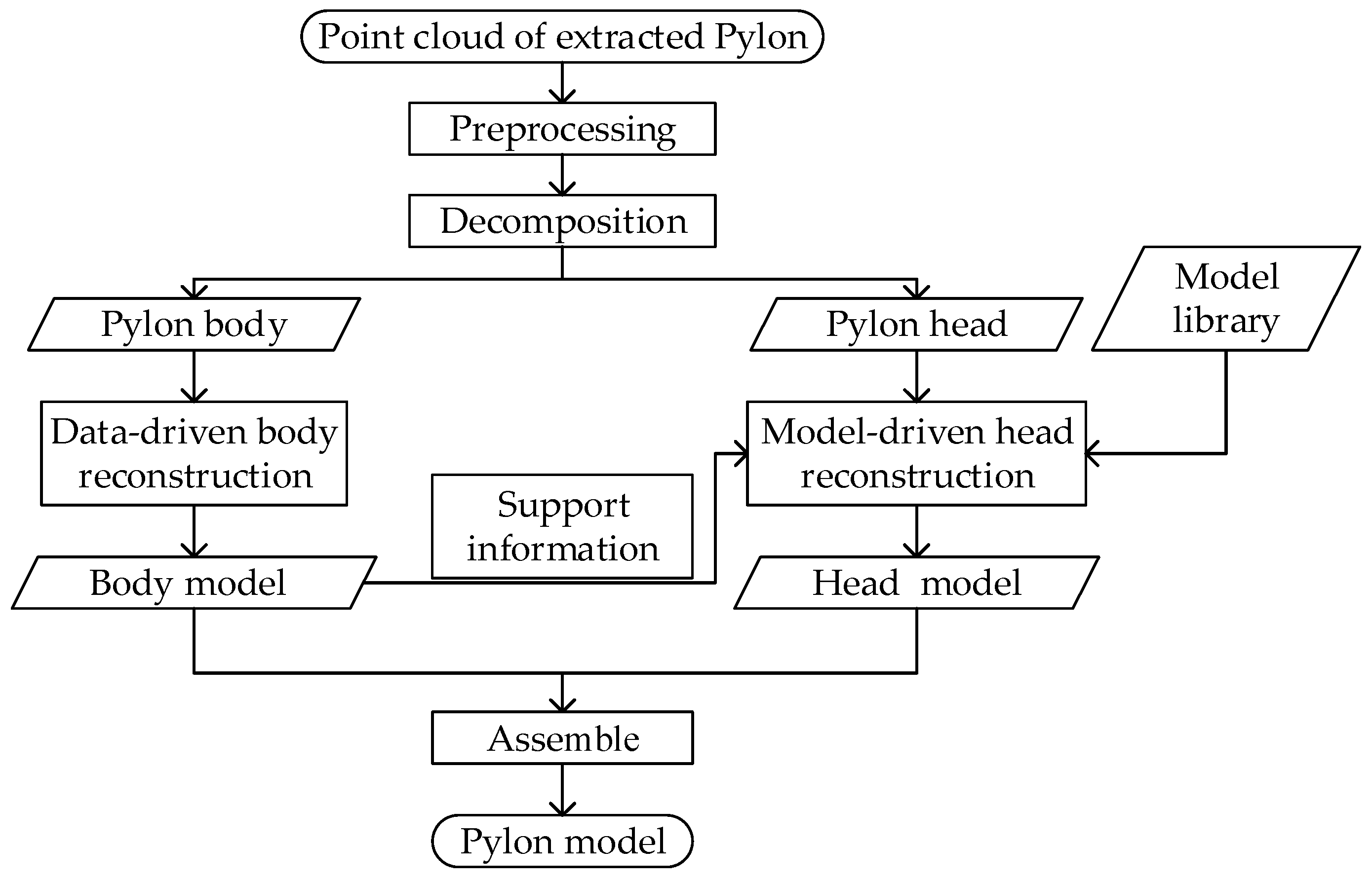
The processing flowchart of the proposed method is shown in Figure 1. Structurally, a pylon is firstly decomposed into two parts: the pylon body and head. Then, optimal strategies are adopted to reconstruct different pylon parts: for the pylon body with a single type and simple structure whose shape is determined by four principal legs, a data-driven method is applied, where a RANSAC-based algorithm is adopted to fit each principal leg with a 3D line; for the pylon head with various types and complex structures, as they are constructed with regular construction constraints, a model-driven method is applied with a predefined model library, where the pylon head type is recognized by a shape context algorithm, and their parameters are estimated by a Metropolis–Hastings (MH) sampler coupled with a Simulated Annealing (SA) algorithm. Body reconstruction results, information about the original point cloud, and geometric relations between parameters are used in the process of head reconstruction to reduce the number and search space of parameters.
1.3. Overview
The rest of the paper is organized as follows. Section 2 introduces the pylon decomposition method and corresponding strategies to reconstruct the pylon body and pylon head. Experimental data and results are, respectively, shown in Section 3 and Section 4. The robustness and influence factors of reconstruction are discussed in Section 5. Finally, conclusions drawn from experiments are presented in Section 6.
2. Methodology
As mentioned in Section 1, according to power pylons’ structure characteristics, the pylon body and pylon head are reconstructed with different strategies. Preprocessing and decomposition methods are firstly introduced in Section 2.1 and Section 2.2. Then, a data-driven strategy based on line features to reconstruct the pylon body is introduced in Section 2.3, while a model-driven strategy to reconstruct the pylon head is introduced in Section 2.4.
2.1. Preprocessing
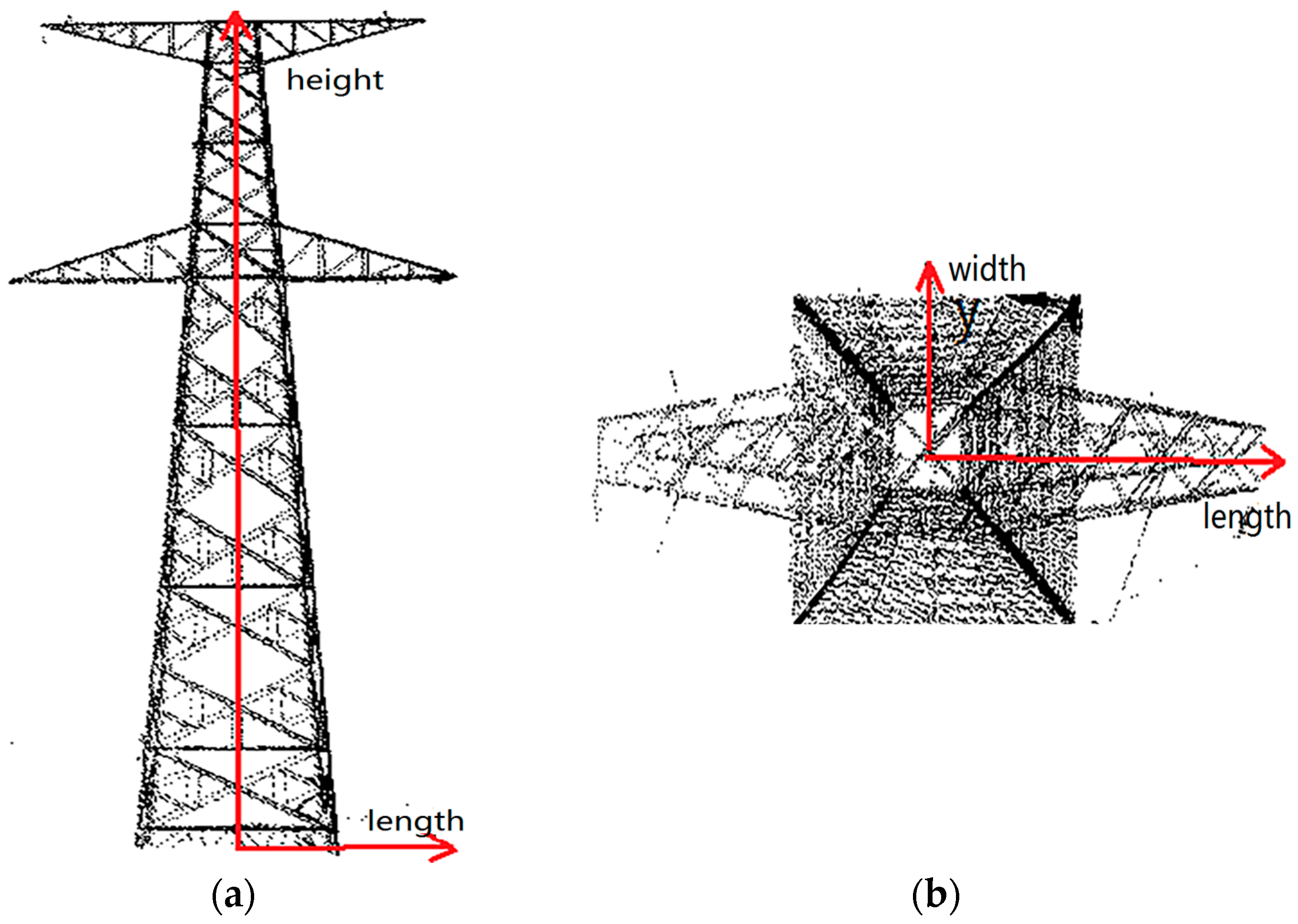
After the point cloud of a pylon is extracted, it can be in arbitrary orientation in the global coordinate system. Before the decomposition and reconstruction of the pylon body and head, the point cloud should be normalized in a convenient 3D pylon coordinate system. The defined 3D pylon coordinate system is located in the bottom center of the pylon body, among three axes of length, width and height, whose definition are illustrated in Figure 2.
Once the 3D pylon coordinate system is established, the point cloud of the pylon can be translated and rotated to a given coordinates system.
2.2. Pylon Decomposition Based on Statistical Analysis
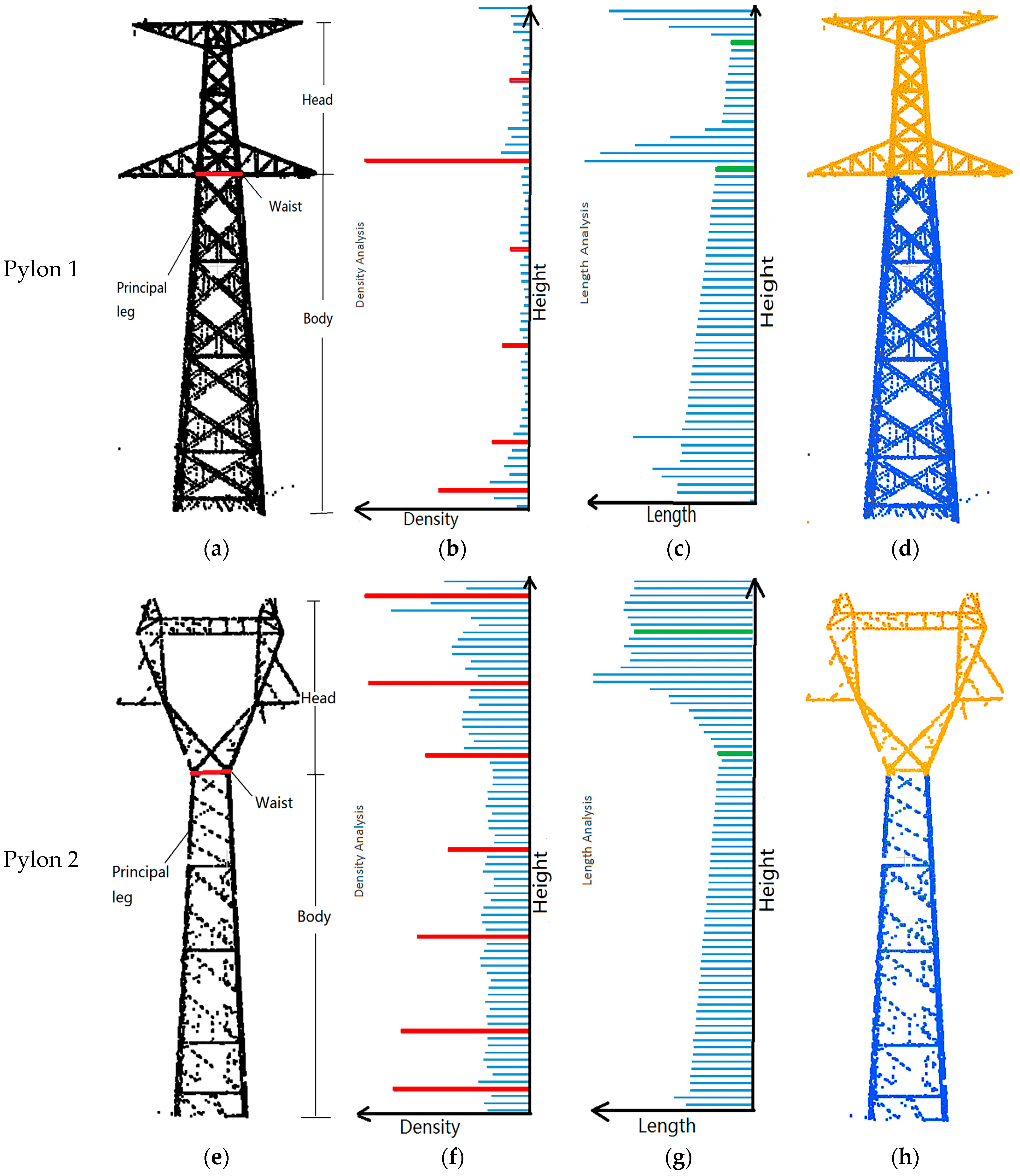
Structurally, a pylon can be decomposed into two parts: the pylon body and head. To explicitly distinguish the pylon body and head, a waist plane is defined, and the part above it is defined as the pylon head while the part below is the pylon body. The waist plane has two types: (1) the low chords of the cross arm in Figure 3a; and (2) the rapidly changed cross-section in Figure 3e.
Although the waist planes’ types are different, there are two common statistical characteristics: (1) the local maximum density used in Li et al. [1]; and (2) the local minimum length. The density is defined as the number of point in each bin, and the length is the maximum distance to the center of each bin. To automatically obtain the waist plane’s height, a statistical analysis on pylon points is carried out.
The pylon points are firstly divided into bins with the equal elevation interval Δh, and each bin’s density and length are calculated to form the density and length histograms. The value of Δh must ensure that each bin contains enough points so that its shape features retained. Next, a forward and backward moving window with the size L × 1 is, respectively, used on both two histograms to find the local maximum density and the local minimum length. As shown in Figure 3b,c, the bins with the local maximum density are colored in red, while the bins with the local minimum length are colored in green. Finally, the bin with both characteristics is automatically extracted as the waist plane, and the position of the bin’s best fitting plane determined by RANSAC is regarded as the waist plane’s height. As shown in Figure 3d,h, the points whose height is under the waist plane’s height are regarded as the body points, while others are head points.
2.3. Pylon Body Reconstruction Based on a Data-Driven Strategy
For the pylon body with a single type and simple structure whose shape is determined by the four principal legs, a data-driven reconstruction method based on line features is applied: corner points of the pylon body are firstly extracted and segmented into four subsets, which is introduced in Section 2.3.1; then, a RANSAC-based algorithm is adopted to fit each subset with a 3D line, and the pylon body model is refined under construction constraints, which are introduced in Section 2.3.2.
2.3.1. Extraction and Segmentation of Corner Points
As principal supporting structures, the size of four principal legs are larger than that of other auxiliary components, leading to the number of points falling on the four principal legs of the pylon body being greater than that of auxiliary components; correspondingly, the color of the four principal legs are darker than other auxiliary components in Figure 4a. Therefore, the line features of four principal legs are opted to reconstruct the pylon body.
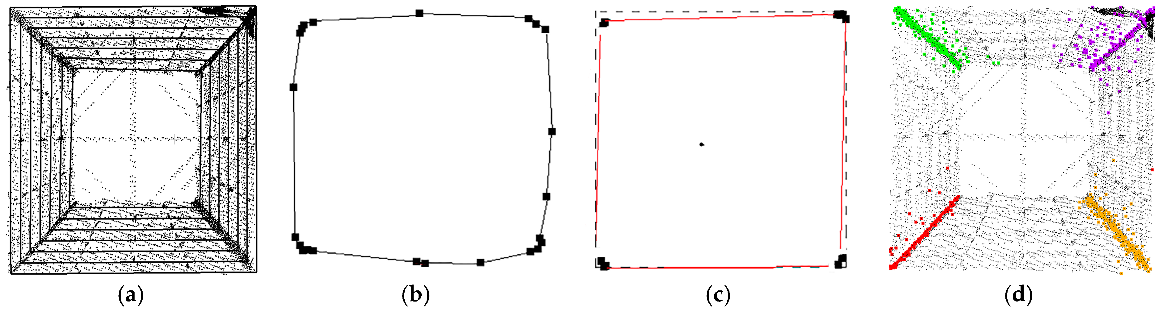
To correctly extract and segment corner points, the pylon body is equally divided into bins in the elevation direction. As shown in Figure 4a, each bin can be viewed as rectangles with the same center from the top view. Those parallel rectangles range from the bottom to the top, and the four corresponding corners of all rectangles are collinear. For each bin, a convex hull algorithm [30] and a polygon simplification algorithm are used to extract corner points [22,23].
At first, the convex hull algorithm is used to construct a contour polygon from points in each bin. As shown in Figure 4b, the contour polygon contains corner points and other points. Then, to detect the corner points, a pipe algorithm [31] is applied to simplify the contour polygon (Figure 4c). Finally, the detected corner points of all bins are segmented into four subsets according to their orientation to the center of the minimum enclosing rectangle (MER). As shown in Figure 4d, each subset of corner points can be approximately described as a 3D line.
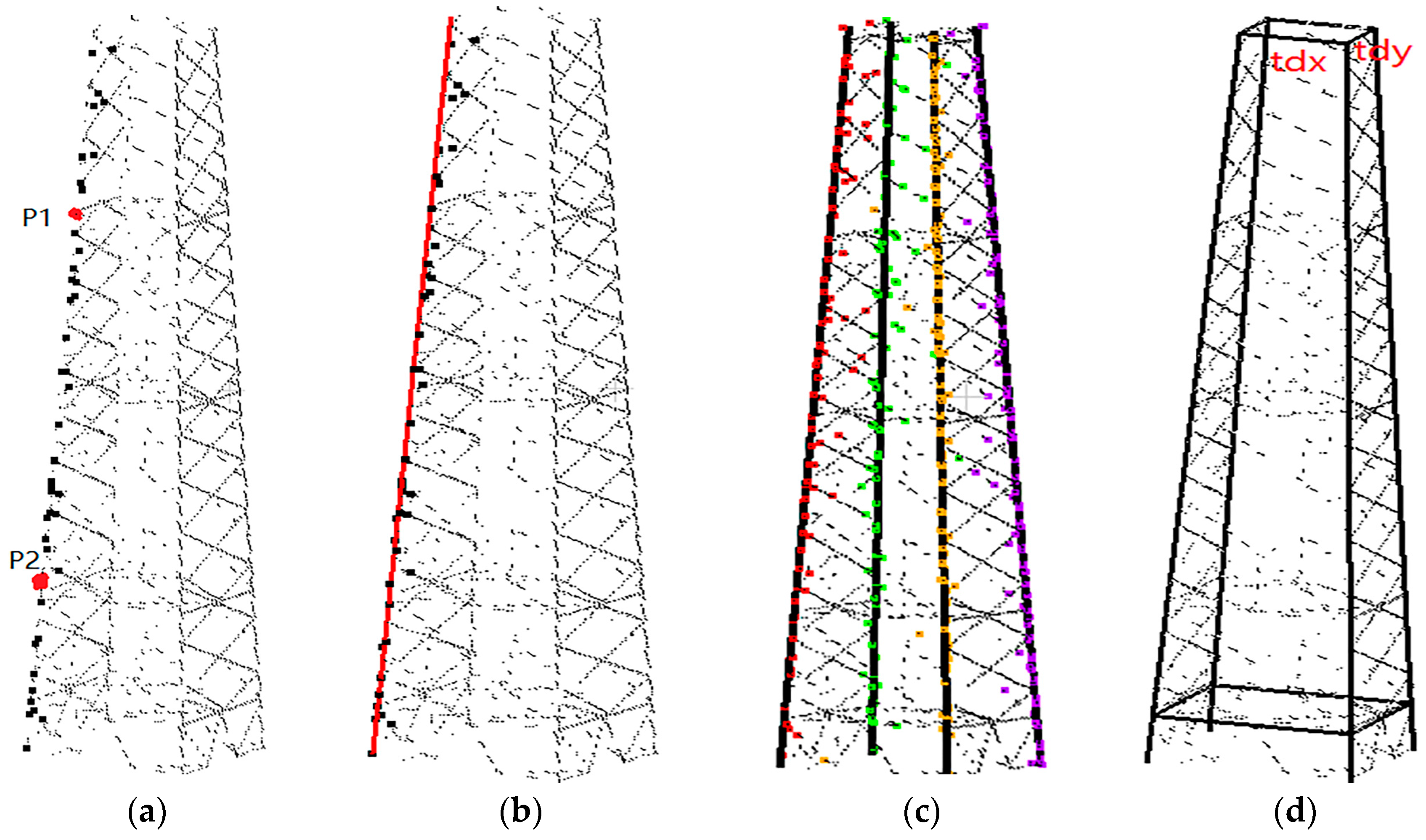
2.3.2. Corner Line Fitting Based on RANSAC
To get corner lines’ equation from corner point set, which might contain non-corner points, a RANSAC-based [32,33] approach is applied. It consists of two key steps: generating a hypothesis by random samples and verifying the hypothesis by the remaining data [34].
Firstly, two points P1 (x1, y1, z1) and P2 (x2, y2, z2) are randomly selected, as shown in Figure 5a. The equation of the 3D line L calculated by the two points is as Equation (1):
Then, the distances from the remaining points to the line L are calculated. If the current point’s distance to the line L is smaller than distance threshold Td, then the current point is defined as the inlier; otherwise, it is defined as the outlier. This process is repeated until a predefined sampling number or some other condition are met, and the line with the most inliers is taken as the final estimation (as shown in Figure 5b).
After the four principal legs are fitted independently (as shown in Figure 5c), three construction constraints are taken into consideration to refine the pylon body reconstruction results: (1) the coplanarity and reflectional symmetry of any two adjacent legs; (2) the reflectional symmetry of any two opposite legs; and (3) the parallelism of the top plane and the bottom plane. The refined reconstruction results of pylon body are shown in Figure 5d. In addition, the pylon body reconstruction results can be used as the constraints in the process of head reconstruction. For example, as shown in Figure 5d, after the body is reconstructed, the length and width of the waist plane can be derived as known parameters tdx, tdy in the pylon head reconstruction.
2.4. Pylon Head Reconstruction Based on a Model-Driven Strategy
For the pylon head with various types and complex structures, as they are constructed with regular construction constraints, a model-driven method is applied: a 3D parametric model library of pylon heads is firstly predefined in Section 2.4.1; and then the type of pylon head is recognized by a shape context algorithm, which is introduced in Section 2.4.2; finally, a Metropolis–Hastings sampler is used to estimate the appropriate parameters of the selected head model with a simulated annealing algorithm, which is introduced in Section 2.4.3.
2.4.1. 3D Parametric Model Library of Pylon Heads
Model-driven methods are based on a predefined model library. In general, although there is little change in the auxiliary or local part of pylon heads, architecturally, most of pylon heads with the same type have the same specific structure, which can be expressed in a unified structural model. By referring to the specification widely used in China for pylon construction, a 3D parametric pylon head model library is predefined.
The integrity of the model library is directly related to the generality of the reconstruction method: if it is too limited, the method loses generality [2]. At present, the model library includes the common pylon heads widely used in high voltage transmission systems in China (shown in Figure 6), as ultrahigh-voltage power-line systems are still under development in China [2]. However, the content of the model library could be widened if required.
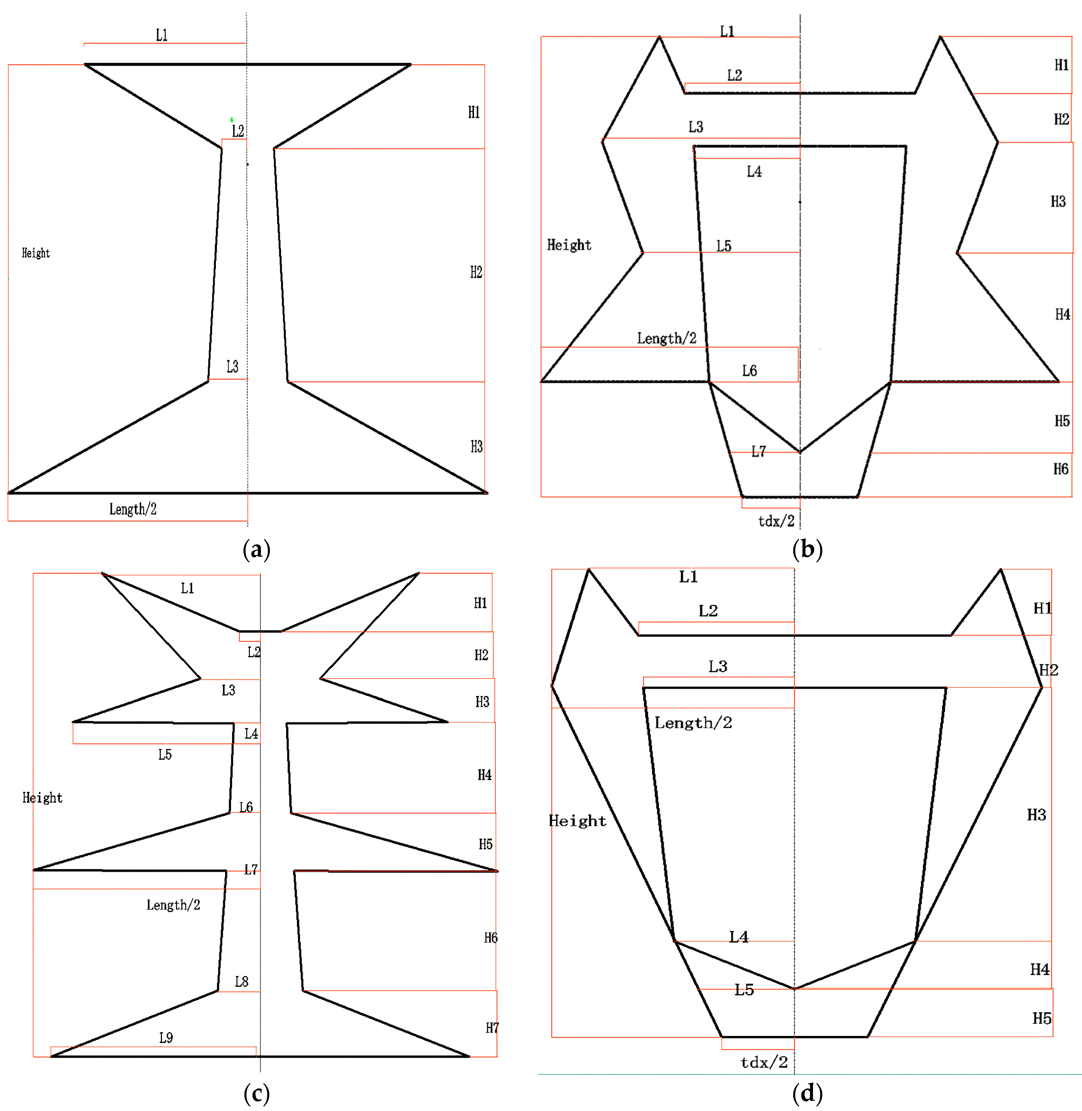
In the model library, the principal components including outer and inner contours are defined. For simplicity, head models in the library are defined with a series of key points, and connected by the predefined relations (such as topological and geometric relations). To get the coordinate of key points, model parameters are specified as the feature height, feature length and feature width. These parameters only give the relative relation of key points and they can be adjusted to fit the data optimally.
As Figure 6 shows, each type is defined with many parameters, which will lead to expensive time cost. To reduce the number of parameters and their search space, the body reconstruction results, information about head points, and geometric relations between parameters are utilized. The parameters of four pylon head models shown in Figure 6 are listed in Table 1. The unknown parameters are the parameters to solve, while the known parameters can be inferred from geometric relations between parameters, information about head points and body reconstruction results.
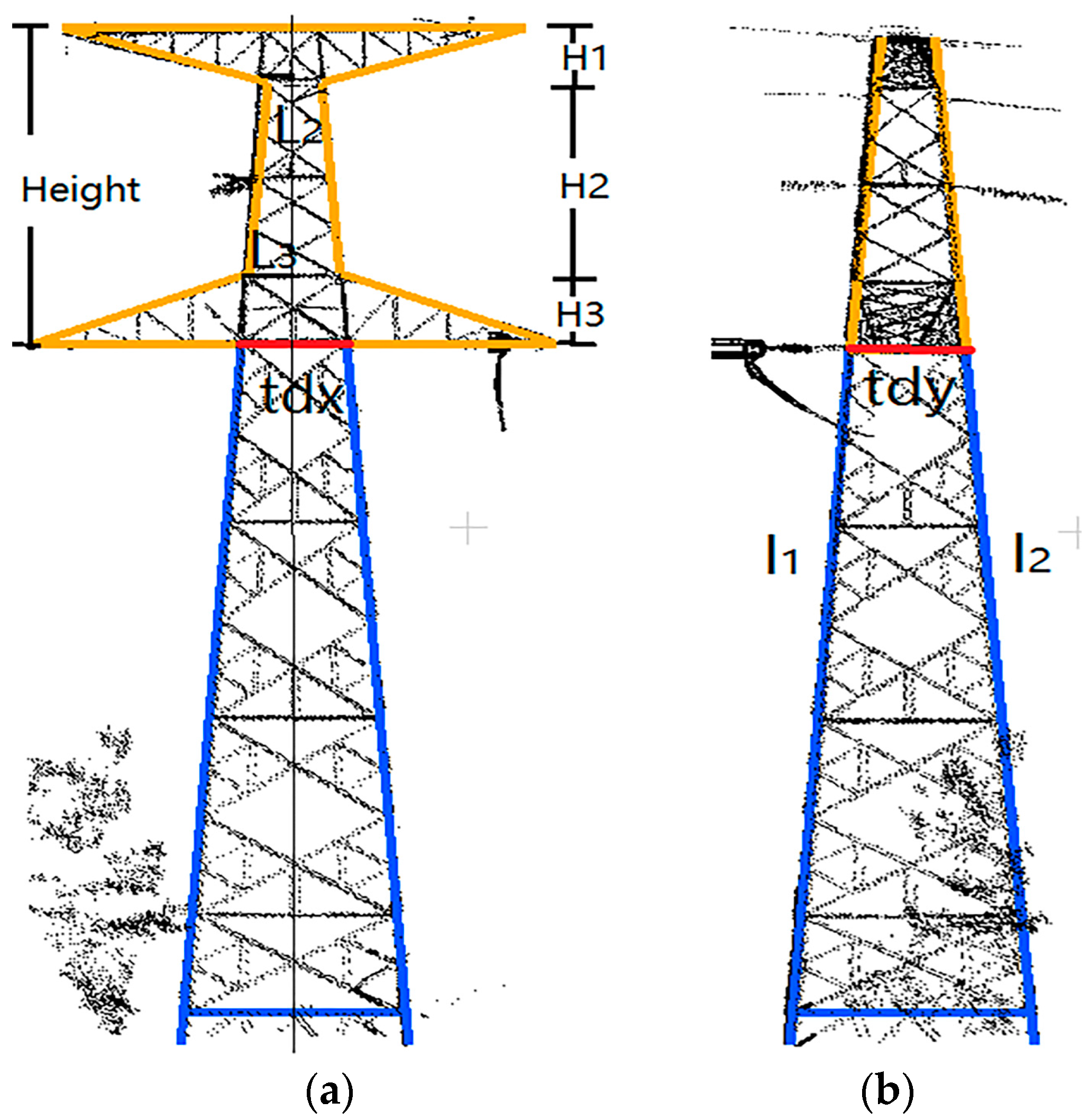
As shown in Table 1, most pylon heads have four basic parameters: tdx, tdy, Height, and Length. tdx and tdy are, respectively, the length and width of the waist plane, which can be derived from the results of body reconstruction as mentioned in Section 2.2. Height and Length are the size of the pylon head, which can be derived from the original pylon head point cloud information. Especially, some parameters can be inferred from other parameters. For example, in Model 1 (as shown in Figure 7a), H3 can be inferred by Equation (2) according to geometric relations, while L3 can be inferred by Equation (3) according to collinearity (in Figure 7a).
The above discussed head models describe only the 2D projection of 3D pylon head on the length-height plane. Another dimension width is also important in the head reconstruction. Similar to length and height parameters, width parameters are used to describe the key points distribution, and some width information about head models can be inferred from the body reconstruction results. As shown in Figure 7b, to make the pylon uniformly stressed, the two contours of pylons head and body are collinear from the side view. After the pylon body is firstly reconstructed (colored in blue), the 3D linear equations of l1 and l2 can be obtained. Then, according to their collinearity, the head width of the side view can be derived.
In addition, the search space of each parameter can also be inferred according to the geometric relations. In this way, the number and search space of parameters is greatly reduced.
2.4.2. Pylon Head Type Recognition by Shape Context
There is a great variation in shape of pylon heads, but they tend to fall into a series of distinct types aimed to recognize. In this step, the head point cloud and rough models are firstly zoomed to the same scale and transformed into binary images, and then a shape context algorithm [35] is applied to recognize the type of pylon head.
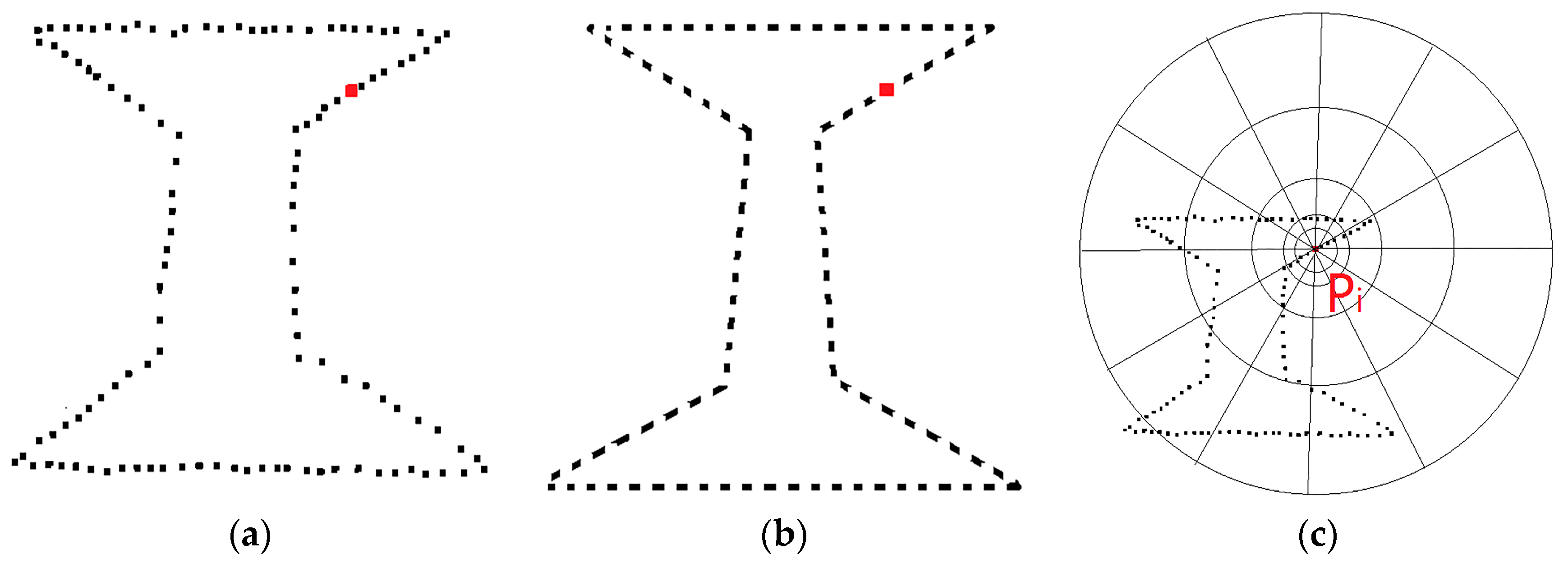
The shape context is a feature descriptor for measuring shape similarity and recovering points correspondences. It has been widely applied in many areas, such as digit recognition, silhouette similarity-based retrieval, trademark retrieval and 3D object recognition. The basic idea is to pick n points P = {p1, p2, p3, …, pn} on each contour of shapes, as shown in Figure 8a,b, and compute the shape context of each point pi. The shape context of pi is defined as the relative coordinates of the remaining n − 1 points. For simplicity, the relative coordinates are replaced with the number of points in each sector of the target template which is shown in Figure 8c. N concentric circles are established at logarithmic intervals in the region where the current point pi is the center and R is the radius, and the region is divided into M bins in a circumferential direction.
To minimize the effect of distortion, a thin plate spline (TPS) transformation that wraps the edges of the model to the point cloud is adopted. Then, the matching cost between each pair of points on the points image and model image are calculated by Equation (4). After the matching cost between each model in the model library and original point cloud are calculated, the model with the minimum total cost is chosen as the right head model.
where Ci,j is the matching cost between point i and point j, hi(k) is the pi’s shape histogram of points, hj(k) is the qj’s shape histogram of models, k = {1, 2, 3, …, K}, and K = M × N.
Because the distribution over relative position is a robust, compact, and highly discriminative descriptor, the shape context is demonstrated to be robust to deformation, noise, and partial data missing. Although the pylon head points are incomplete and distorted, this method accurately recognizes the pylon head’s type from other model types by finding the minimum total matching cost.
2.4.3. Optimizations
In this section, the pylon head reconstruction process is transformed into a Gibbs energy optimization issue. Gibbs energy is defined as the similarity between the raw pylon head points and the head model. To find the approximate solution of model parameters, the Metropolis–Hastings sampler is adopted coupled with simulated annealing algorithm.
(1) Gibbs Energy
The Gibbs energy function [2] is used to quantitatively evaluate the similarity between the reconstructed head model and original point cloud. To reduce the deviation caused by the local optimum, the similarity u(x) consist of two simple distance: the average distance from model to head points and the average distance from head points to model .
a + b = 1. a and b are two weights which represent the contribution to the energy.
The shape of pylon head is determined by the inner contour and outer contour. To reduce the effect of non-contour points, the key points of model and head points on the contours are extracted by alpha shape algorithm [36]. Thus, the distance is simplified as the average distance from each model key point to the closest head point (Equation (7)), while is average distance from each head key point to the closest model point (Equation (8)). Through minimizing the Gibbs energy, the head points and the model can be well matched.
where n is the number of model key points, and m is the number of head key points.
(2) Metropolis–Hastings and simulated annealing algorithms
As the most popular Markov Chain Monte Carlo (MCMC) method, Metropolis–Hastings (MH) algorithm is widely adopted to estimate the approximate value of model parameters. The key idea is that through statistical sampling, a complex combination problem can be approximated by a much simpler problem [8]. Target distribution and proposal distribution are involved in the MH sampling process. Firstly, a candidate value of the current value x is sampled in space X according to . Then, the acceptance probability is calculated by Equation (9). If the acceptance probability is bigger than the predefined threshold, then, the Markov chain will move towards ; otherwise, it rejects and remains at x. By constantly sampling, the value tends to converge.
In this paper, a Gaussian distribution is selected as the proposal distribution, and the Gibbs energy is set as the target distribution. Due to the symmetry of the proposal distribution, the is equal to , therefore, the acceptance ratio is simplified as Equation (10).
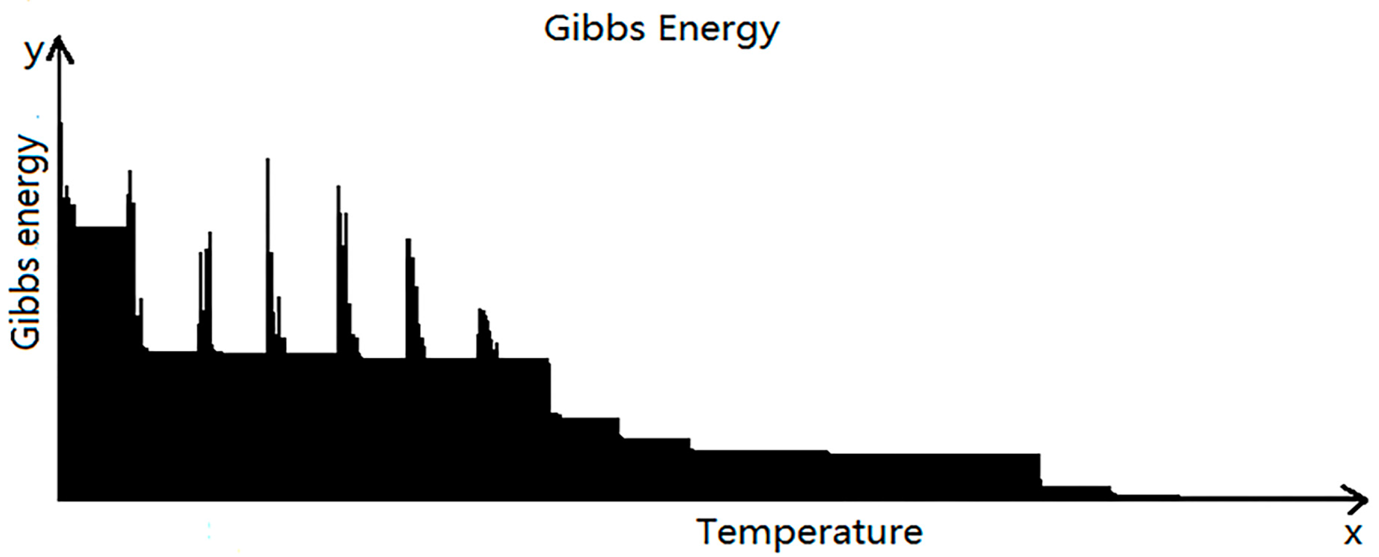
The MH sampler is of low efficiency, because random samples are rarely from the proximity of the mode [8]. To make the sampling procedure more efficient, the simulated annealing (SA) algorithm is used, whose target distribution at iteration i is instead of in MH sampler. The annealing process starts with a high initial temperature (T0 = 1), and the decreasing cooling schedule Ti is required as [8]. As shown in Figure 9, with the temperature Ti cooling, the probability of accepting worse solutions explored in the search space will decrease. When the temperature T is low enough, the target distribution eventually tends to be global optimal as it can jump out the local optimal solution with high probability.
Most convergence results for simulated annealing typically state that, if for a given Ti, the homogeneous Markov transition kernel mixes quickly enough, then convergence to the set of global maxima of is ensured for an appropriate sequence Ti. To cool the temperature T quickly, an exponential cooling schedule is chosen. Combining the Gibbs energy and the MH sampler, the detailed procedure of simulated annealing is shown in the Appendix A.
3. Experimental Data
To verify the feasibility of the proposed method, a set of experiments are conducted on the LiDAR data of power pylons, which were collected from Guangdong Province, China. The original point cloud data were collected by a Riegl VUX-1 laser measurement system. Details about data acquisition are shown in Table 2.
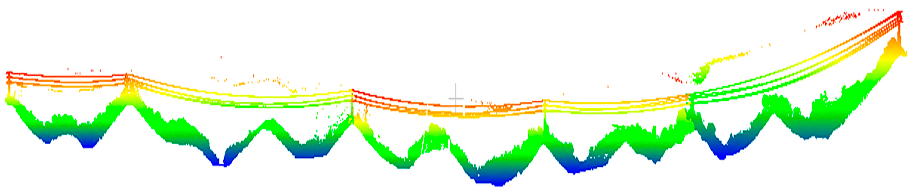
The average distance of the original point cloud used in the experiments is about 0.05 m. An example area of the original data is shown in Figure 10. The size of the shown transmission corridor is about 1881 × 40 m2, and the points amount is 43,879,821, including six power pylons. The point density of the example area is about 500 pts/m2 on average.
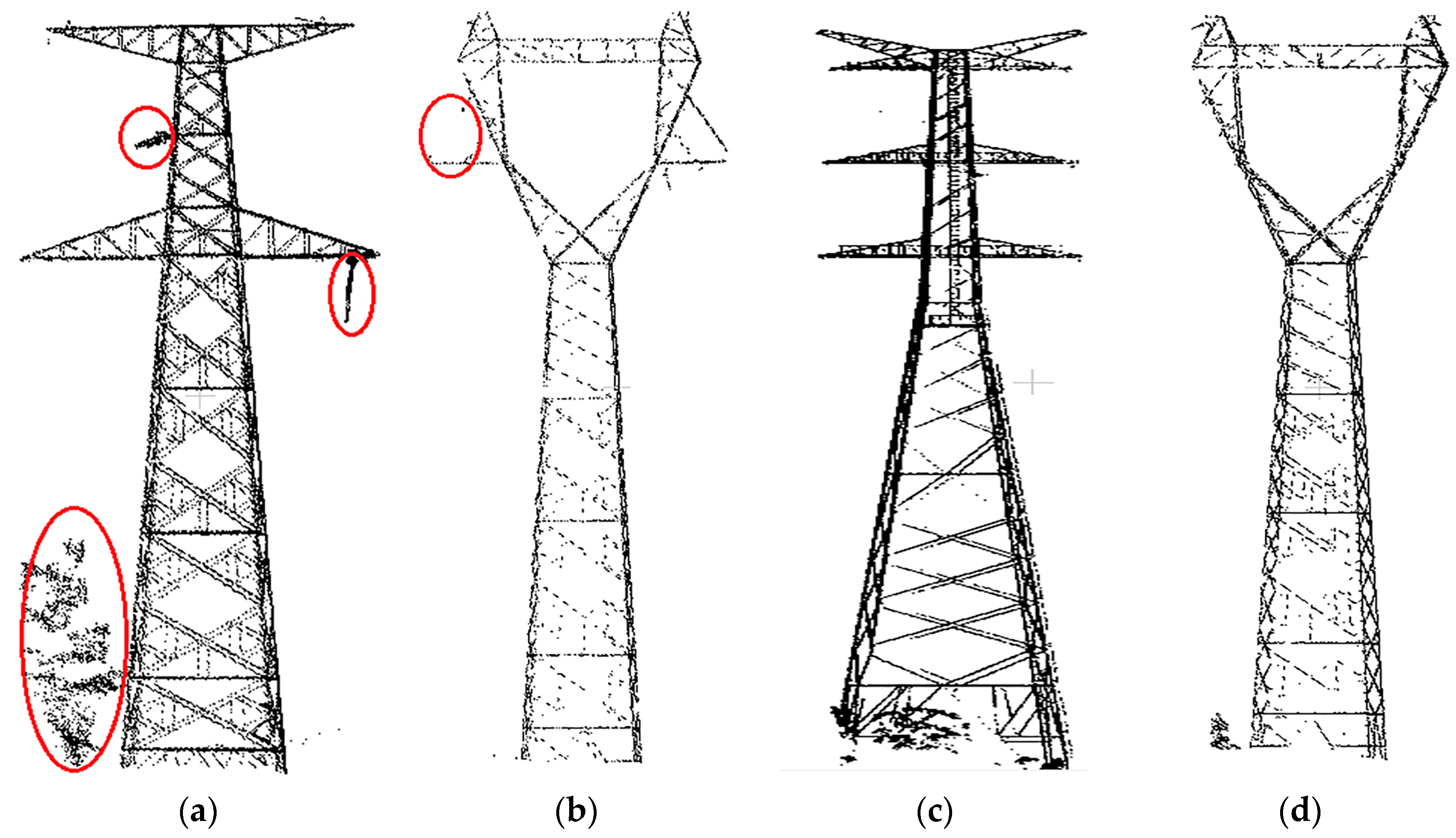
In the experiments, the point cloud of power pylons is firstly extracted from the original data by software, and then they are transformed to the pylon coordinate system automatically. Four typical extracted pylons are shown in Figure 11. As shown in Figure 11a, after the pylon is extracted, there are some vegetation and power line points around the pylons, which may influence the reconstruction results. As shown in Figure 11b, some data are missing, which will lead to partial reconstruction deviation. The pylon bodies of four types approximately are quadrangular frustum pyramids, and their shapes are determined by four principal legs. The pylon heads are more varied in shape and parameters of each type are different, adding complexity to head reconstruction.
4. Results
In this Section, experiments are conducted on power pylons of several transmission lines with the proposed method, and the results are shown as follows: the accuracy of pylon decomposition is firstly listed in Section 4.1; then, the pylon body reconstruction accuracy is shown in Section 4.2; the head type recognition results are shown in Section 4.3; and the accuracy and efficiency of pylon head reconstruction are, respectively, listed in Section 4.4 and Section 4.5.
4.1. Decomposition Results of Different Pylon Types
Decomposition of the power pylon into the body and head is a basic step of the process, and it is directly related to the correctness of final reconstruction. To verify the proposed method, it is applied to data comprising four types of pylon, and each type has 10 examples. Then, the height of 10 pylons’ waist plane is compared with the height extracted interactively in CloudCompare. When the elevation interval Δh of each bin is set to 0.3 m and the distance threshold of plane fitting based on RANSAC is set to 0.1 m, the correctness of the waist plane extraction and the average error dh of waist planes’ height is listed in Table 3, while the correctness is the ratio of the correctly decomposed pylons’ amount to the total pylons’ amount of the same type.
In the experiment, two pylons are decomposed incorrectly, both due to the unfiltered power line points around the waist plane. They are both correctly decomposed after the unfiltered power line points are manually removed. Results indicate that the decomposition method based on statistical analysis is feasible, and most waist planes of different types are correctly identified, and the location error of the waist plane is less than 0.10 m.
4.2. Precision of Pylon Body Reconstruction
In this experiment, the proposed data-driven method to reconstruct the pylon body is applied to the 40 decomposed pylons. To evaluate the feasibility of the method, the fitting residual between the extracted corner points and fitting lines, and related accuracy between the reconstructed model and the original point cloud of pylon body are calculated.
To evaluate the fitting accuracy of the extracted corner points, the number of extracted corner points Ni, the ratio of inliers ri, and the fitting residual of each leg i between the fitted line and inliers of extracted corner points are calculated. The fitting residual is defined as Equation (11):
where is the distance of inlier pk to the fitting line L, and n is the number of inliers.
Table 4 shows the fitting residual of 12 randomly selected pylons from four types. The distance threshold Td is set to 0.1 m. Table 4 demonstrates that the maximum fitting residual of each leg is 0.022 m, and the accuracy of body reconstruction is not related to pylon types.
To visually check the results of pylon body reconstruction, the original point cloud of pylon body and reconstruction results are shown in Figure 13. The reconstruction results are colored in blue, while the original point cloud is in black. It can be seen from both front and side views that the reconstructed body models are in good agreement with four principal legs in shape.
To give a quantitative precision of the reconstructed body models, related accuracy between the reconstructed model and the original point cloud are measured in the CloudCompare, which is defined as the maximum 2D distance from the pylon points to the four reconstructed legs in the front and side projected plane. The results of the 12 pylon bodies are listed in Table 5. The maximum and average 2D distance to the front plane is 0.153 m and 0.061 m while the maximum and average distance to the side plane is 0.109 m and 0.072 m, and they are sufficiently accurate to meet the requirements of 3D digitalization.
4.3. Recognition of Pylon Head Type
In this experiment, 12 selected pylons mentioned in Section 4.2 are tested. All heads types are correctly recognized by the shape context algorithm, and the matching cost of four randomly selected models are listed in Table 6.
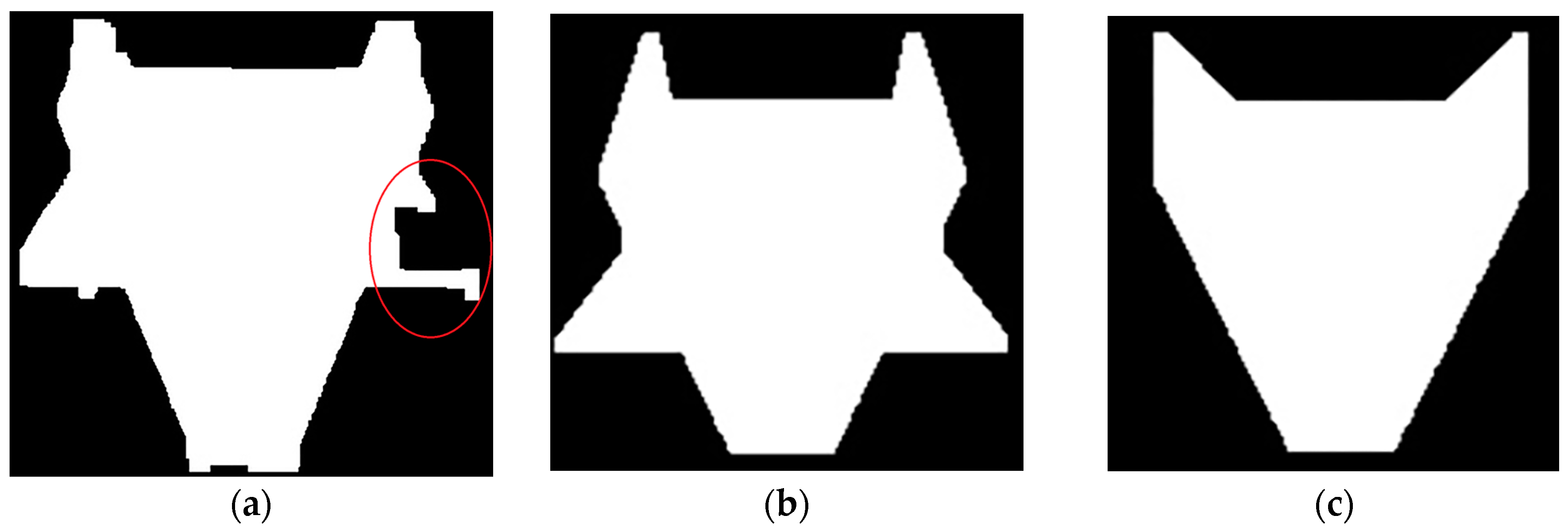
Among the four pylon heads, the head of pylon 3 (Figure 12a) has a big data loss in the right side, whose matching cost to Model 2 (Figure 12b) and Model 4 (Figure 12c) are both small, but the ratio of the smallest cost and the second smallest cost reaches 0.76, still robust enough to choose the Model 2 as the right model. The experiment shows that the shape context algorithm can robustly identify the four typical pylon head types even with deformation, noise, and partial data missing.
4.4. Precision of Pylon Head Reconstruction
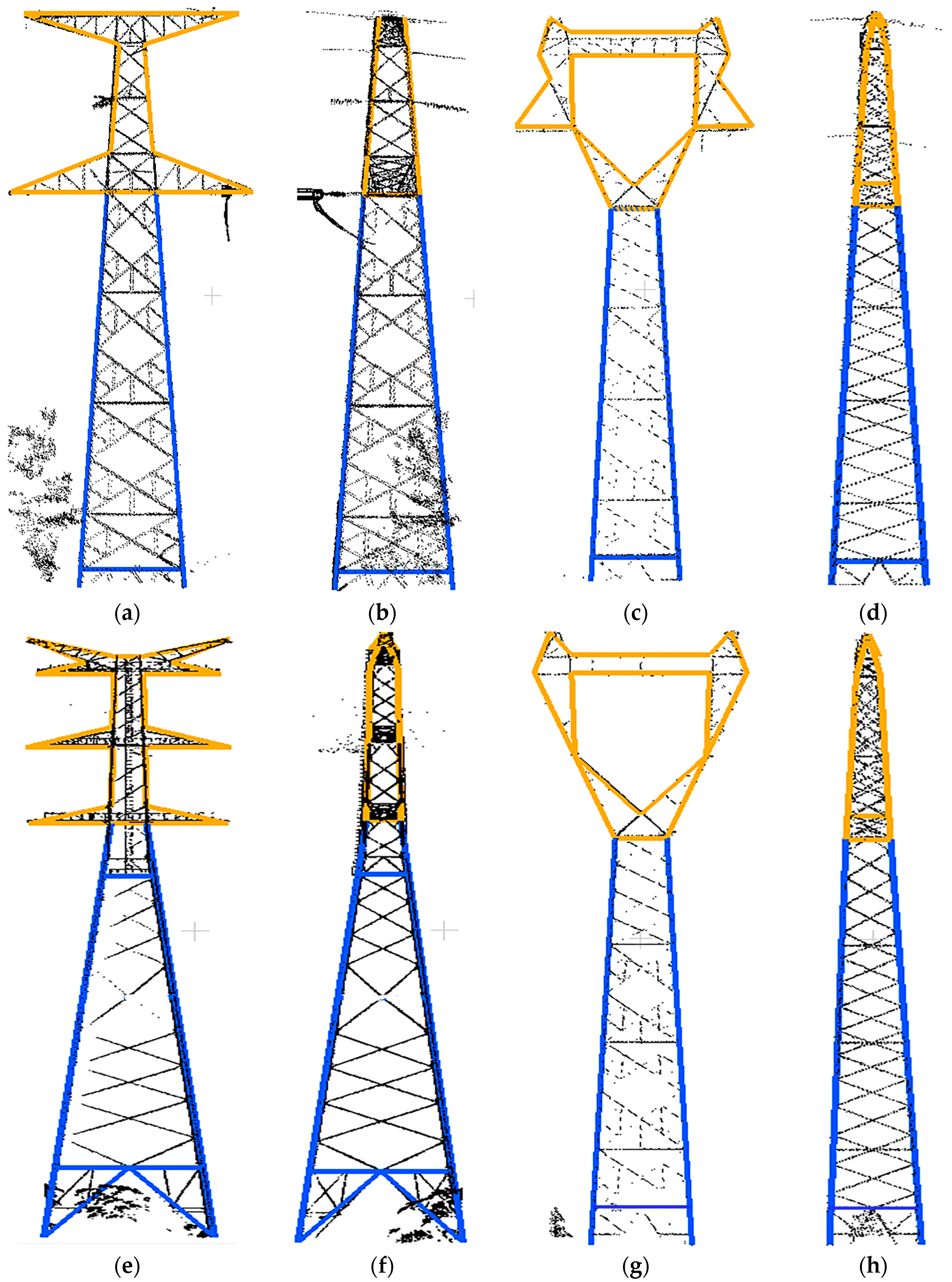
In this experiment, 12 selected pylons mentioned in Section 4.2 are tested to verify the feasibility of the head reconstruction method. To make reconstruction results clearly visible, four typical pylons’ reconstruction results are shown in Figure 13, where the reconstructed head models are colored in yellow and the original pylon points are in black. As shown in Figure 13, all reconstructed pylon head models are attached to the original point cloud well, even with noise, and partial data missing.
To quantitatively evaluate the accuracy of head reconstruction results, the number of key points extracted by an alpha shape algorithm ncount, the average distance Dave and maximum distance Dmax between the reconstructed head model and the original point cloud are, respectively, calculated according to Equations (12) and (13).
where dis(pi, qi) is the distance from the model key points pi to the corresponding closest point qi of the original pylon point cloud, and n is the number of model key points.
The head reconstruction accuracy of four typical pylons (shown in Figure 13) are listed in Table 7. For the four pylon heads, 522 key points of the original head point cloud are extracted by an alpha shape algorithm on average. The average distance Dave of four pylon heads is 0.196 m on average, while the maximum distance Dmax of the four pylon heads is 0.333 m.
4.5. Efficiency of Pylon Head Reconstruction
To evaluate the efficiency of the head reconstruction method, 12 selected pylons mentioned in Section 4.2 are tested on an Intel Core i7-6770HQ PC on an ASUS notebook powered by Intel Core i7-6770HQ 2.6 GHz CPU. The number of unknown parameters Np (mentioned in Section 2.3.1), the head size of original point cloud, the number of points ncount, and the time consumption Time are calculated. Table 8 shows the reconstruction time of the 12 pylons, which is sorted by Time.
As Table 8 shows, the time consumption of the head reconstruction is mostly determined by the head type and size, as the various types lead to different numbers of parameters, while the head size is related to the search space of parameters. As the number of unknown parameters increases, more running time is required to estimate the appropriate value of parameters. For pylon heads with the same type, the time consumption has a slight fluctuation, which is affected by the search space of parameters, and the larger the search space is, the more reconstruction time is required.
As the proposed head reconstruction method makes use of the body reconstruction results, information about the original point cloud, and relationships between parameters to reduce the number of parameters and their search space, the head model is efficiently reconstructed. However, due to the limitation of the model library, the model-driven method is not suitable to reconstruct pylon heads whose type is not predefined in the model library, especially in different countries or different rank power transmission systems. Because the pylon heads are usually constructed with specification and the models can be parameterized [2], the updating of library can be done conveniently. After the new types of pylon heads have been added in the model library, the pylon can be efficiently and precisely reconstructed.
5. Discussion
In this section, the robustness of the proposed body reconstruction method will be analyzed in Section 5.1, and the factors that influence the pylon head reconstruction accuracy will be discussed in Section 5.2.
5.1. Robustness to Noise of Pylon Body Reconstruction
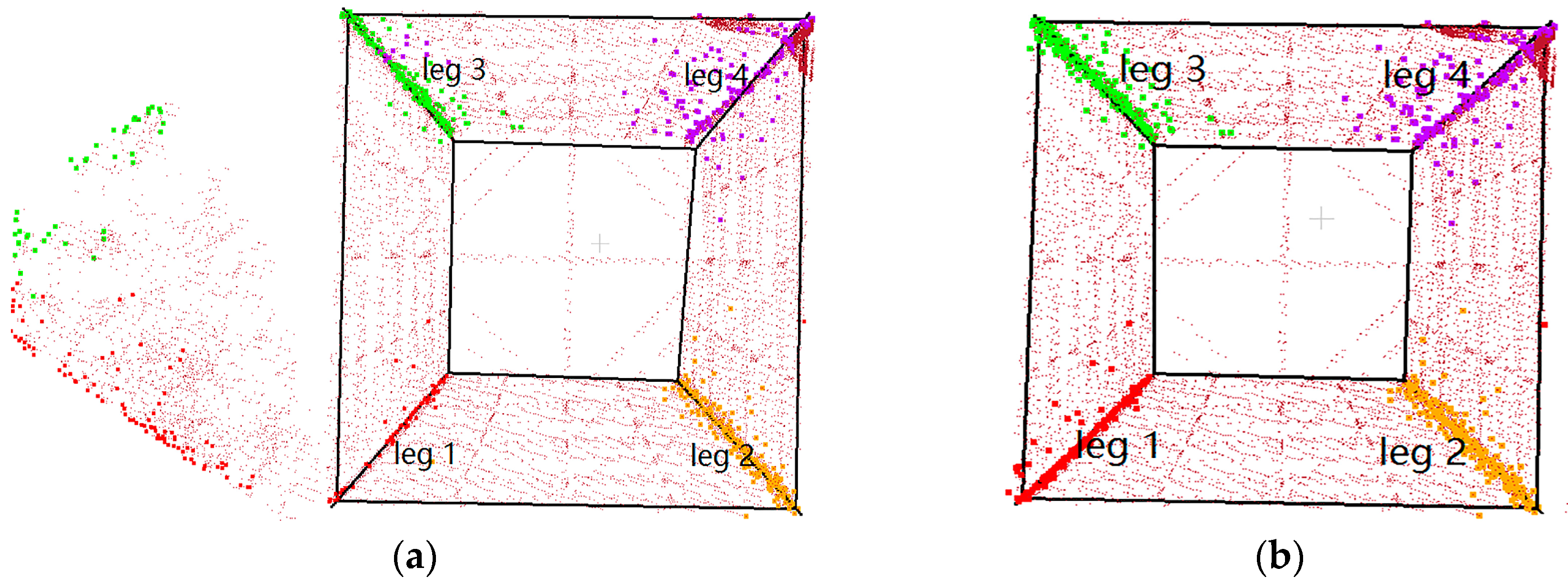
Bad pylon body reconstruction results are usually caused by the sparseness or incompleteness of the original point cloud, or points that do not belong to pylon such as vegetation or power line points. As Figure 14a shows, there are many unfiltered vegetation points around leg 1 and leg 3 of the pylon body. When extracting the corner points of pylon body, the vegetation points can also be extracted, which will lead the inliers ratio of the effected legs being much lower than the unaffected legs. Figure 14b shows the body reconstruction results of the same pylon after the vegetation points are manually filtered. Without vegetation points effect, more corner points are correctly extracted and participate in the body reconstruction, which results in higher confidence and accuracy.
To evaluate the influence of unfiltered vegetation points, the accuracy of the pylon body in the two situations are calculated and shown in Table 9. For the situation in Figure 14a, the inliers ratio of the two affected legs (leg 1 and leg 3) are only 40% and 37%, while the two unaffected legs (leg 2 and leg 4) are up to 74% and 63%. For the situation in Figure 14b, without the effect of vegetation points, the inliers ratio of leg 1 is up to 83%, which is much more than 40%. However, the fitting deviation of leg 1 in the two situations is very small, which only changes from 0.008 m (with noise) to 0.006 m (without noise). A conclusion can be drawn obviously that the noise leads to low inliers ratio, but has a very small impact on the fitting residual.
From the comparison, a conclusion can be drawn that the RANSAC-based algorithm to reconstruct pylon body is robust to noise. It can robustly solve parameters of a certain mathematical model even from data containing a large amount of noise, and noise tends to have small or no influence on the values.
5.2. Influence Factors of Pylon Head Reconstruction
Theoretically, the pylon head reconstruction results are affected by the reconstruction method and data quality. Therefore, in this section, two typical influence factors will be analyzed: (1) key points extraction; and (2) data loss.
5.2.1. Key Points Extraction
Key points extraction is quite important in the pylon head reconstruction process. If the extracted key points can well represent the inner and outer contour of pylon head shape, the result is ideal; otherwise, the deviation will occur. To compare the effect of key points extraction results on the head reconstruction, three alpha values of the alpha shape algorithm are applied, and the extracted key points and reconstructed models are shown in Figure 15.
As shown in Figure 15 and Table 10, as the alpha value decreases from 1 m to 0.1 m, more and more non-contour points are extracted as key points; especially when the alpha value is 0.1 m, almost all points (1077) are extracted as contour points. Correspondingly, with the alpha value decreasing, the average distance Dave between the reconstructed models and the original point cloud increase from 0.176 m to 0.244 m, while the maximum distance Dmax increases from 0.274 m to 0.435 m, showing that the quality of reconstructed model also decreases. Thus, the alpha value should be selected carefully to capture the detail of head contour while not introducing non-contour points.
5.2.2. Data Loss
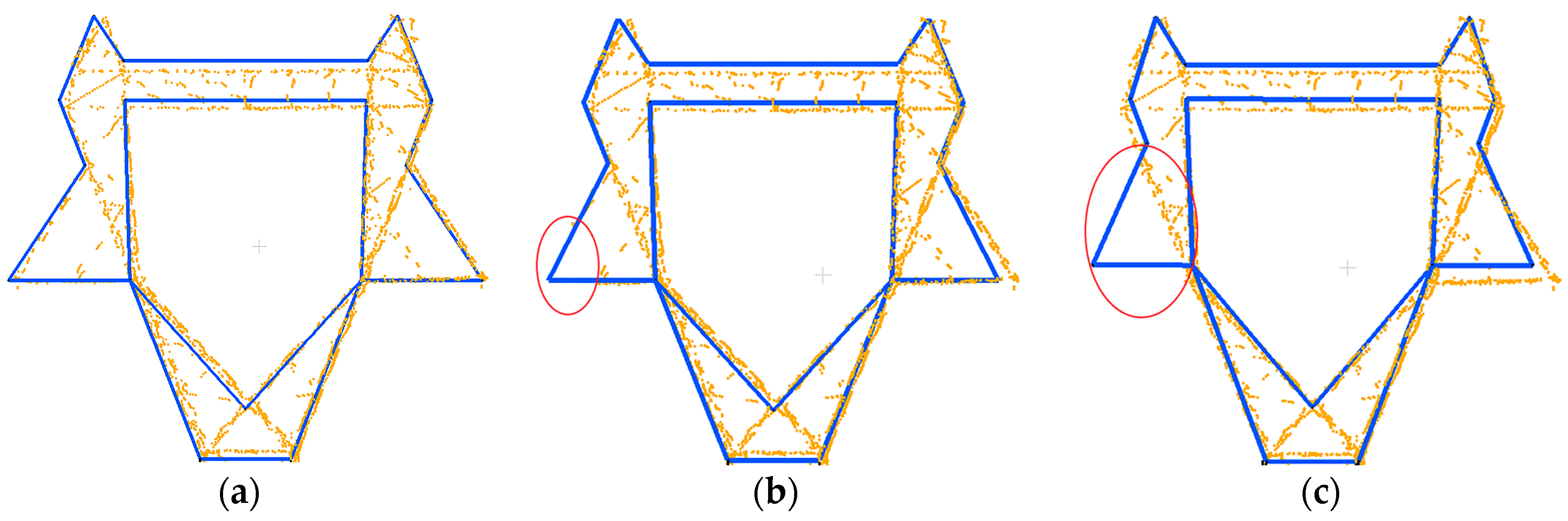
To test the method’s sensitivity to data loss, three levels of data loss are tested. In Figure 16, the point cloud in Figure 16a is complete without data loss; in Figure 16b, some points are missing but do not affect the completeness of head structure; and, in Figure 16c, the whole points of the left section are missing.
The reconstruction result in Figure 16a is closest to the original points, as all contour information of the pylon head is reserved. In Figure 16b, it is clearly shown that the difference between Figure 16a,b is small. This is because the topological constraint relationships, such as parallel, symmetric, have already been implied when defining the models, which makes the reconstruction model with high regularization. In Figure 16c, the structure of the model is still correct but the details of reconstruction are not precise. It is because that pylon parts with few points contribute little to the data coherence term in the energy calculation. The MH sampler and simulated annealing usually cannot find an absolute optimization.
6. Conclusions
In this paper, a heuristic pylon reconstruction method combining both data-driven and model-driven strategies is introduced. Compared with existing pylon reconstruction methods, the proposed method has several characteristics, and shows potential in pylon reconstruction from LiDAR data. The major contributions of the proposed method mainly exist in four aspects: (1) using the statistics analysis method, which combines both the local maximum density and the minimum length, to automatically decompose a pylon into body and head which is more applicable than Li et al. [1] method for various pylon types; (2) reconstructing the pylon body and head with optimal strategies, which are robust to noise and partially missing data; (3) the flow of body reconstruction method is simpler than Li et al. [1], using a RANSAC based 3D line fitting method to reconstruct four principal legs of a pylon body, improving the stability of body reconstruction, which can also ensure the reconstruction accuracy; and (4) using a shape context algorithm to recognize the head type, and a Metropolis-Hastings (MH) sampler coupled with Simulated Annealing (SA) algorithm to solve the head parameters, improving the robustness of head type recognition while reducing the parameters of optimization. Meanwhile, pylon body reconstruction results and the original point cloud information are utilized in the model parameters solving process. Overall, the pylon reconstruction results are accurate and efficient for 3D digitalization.
However, the proposed method also has some limitations. One is that this method is only applicable for pylons with four legs, and the pylon head reconstruction results are limited by the integrity of the predefined model library. As the pylon head types vary greatly in different situations, the head model library should be widened and new pylon head models should be introduced into the library to ensure the integrity of the model library. An extra effort should be applied to determine the generalization of the proposed approach to model different pylon structures and different pylons. In addition, the proposed method currently only focuses on the reconstruction of principal pylon components, which is the first and most important work in the digitalization of power pylon. Next, the reconstruction of material size and auxiliary structure will be considered, which is useful to improve the 3D visualization effect. Meanwhile, multi-platform multi-sensor data, such as terrestrial laser scanning and optical image, can be introduced to reconstruct the power more accurately, and in more detail. In addition, as the first step of pylon and power line reconstruction, automatic classification and extraction of point cloud data will be studied to improve the automation of the whole procedure.
Acknowledgments
The authors would like to express their gratitude to the editors and the reviewers for their constructive and helpful comments for substantial improvement of this paper. This work was supported by the Key Technology program of China South Power Grid under Grant GDKJQQ20161187. The dataset was provided by the patrol operation center of Guangdong Power Grid Co., Ltd.
Author Contributions
Ruqin Zhou and Wanshou Jiang contributed to the study design and manuscript writing. Ruqin Zhou and Wei Huang conceived and designed the experiments. Bo Xu contributed to the analysis tools and partial codes of the algorithm. San Jiang contributed significantly to the discussion of the results and manuscript refinement.
Conflicts of Interest
The authors declare no conflict of interest.
Appendix A. Detailed Procedure of Simulated Annealing Algorithm
| Input: space X, original state x0, initial temperature T, iteration number N at each temperature and the cooling rate γ |
| While T > Tmin |
| { |
| For i = 0 to N |
| sample x* according to in space X |
| if > random (0, 1) |
| xi+1 = x*; |
| else |
| xi+1 = xi; |
| T = T*γ; |
| } |
References
- Li, Q.; Chen, Z.; Hu, Q. A model-driven approach for 3d modeling of pylon from airborne LiDAR data. Remote Sens. 2015, 7, 11501–11524. [Google Scholar] [CrossRef]
- Guo, B.; Huang, X.; Li, Q. A Stochastic Geometry Method for Pylon Reconstruction from Airborne LiDAR Data. Remote Sens. 2016, 8, 243. [Google Scholar] [CrossRef]
- Conde, B.; Villarino, A.; Cabaleiro, M.; Gonzalez-Aguilera, D. Geometrical issues on the structural analysis of transmission electricity towers thanks to laser scanning technology and finite element method. Remote Sens. 2015, 7, 11551–11569. [Google Scholar] [CrossRef]
- Cabaleiro, M.; Riveiro, B.; Arias, P. Automatic 3D modelling of metal frame connections from LiDAR data for structural engineering purposes. ISPRS J. Photogramm. Remote Sens. 2014, 96, 47–56. [Google Scholar] [CrossRef]
- Han, W. Three-Dimensional Power Tower Modeling with Airborne LiDAR Data. J. Yangtze River Sci. Res. Inst. 2012, 29, 122–126. [Google Scholar]
- Chen, Z.; Lan, Z.; Long, H.; Hu, Q. 3D modeling of pylon from airborne LiDAR data. In Proceedings of the SPIE 9158, Remote Sensing of the Environment: 18th National Symposium on Remote Sensing of China, 915807, Wuhan, China, 20–23 October 2012. [Google Scholar]
- Kwoczyńska, B.; Dobek, J. Elaboration of the 3D Model and Survey of the Power Lines Using Data From Airborne Laser Scanning. J. Ecol. Eng. 2016, 17, 65–74. [Google Scholar] [CrossRef]
- Andrieu, C. An Introduction to MCMC for Machine Learning. Mach. Learn. 2003, 50, 5–43. [Google Scholar] [CrossRef]
- Zheng, Y.; Weng, Q.; Zheng, Y. A Hybrid Approach for Three-Dimensional Building Reconstruction in Indianapolis from LiDAR Data. Remote Sens. 2017, 9, 310. [Google Scholar] [CrossRef]
- Zhu, L.; Lehtomaki, M.; Hyyppa, J.; Puttonen, E.; Krooks, A.; Hyyppa, H. Automated 3D reconstruction from open geospatial data sources: Airborne laser scanning and a 2D topographic database. Remote Sens. 2015, 7, 6710–6740. [Google Scholar] [CrossRef]
- Xu, Y.; Yao, W.; Hoegner, L. Segmentation of building roofs from airborne LiDAR point clouds using robust voxel-based region growing. Remote Sens. Lett. 2017, 8, 1062–1071. [Google Scholar] [CrossRef]
- Wu, T.; Hu, X.; Ye, L. Fast and accurate plane segmentation of airborne LiDAR point cloud using cross-line elements. Remote Sens. 2016, 8, 383. [Google Scholar] [CrossRef]
- Chen, D.; Zhang, L.Q.; Li, J.; Liu, R. Urban building roof segmentation from airborne LiDAR point clouds. Int. J. Remote Sens. 2012, 33, 6497–6515. [Google Scholar] [CrossRef]
- Xu, B.; Jiang, W.; Shan, J.; Zhang, J.; Li, L. Investigation on the Weighted RANSAC Approaches for Building Roof Plane Segmentation from LiDAR Point Clouds. Remote Sens. 2016, 8, 5. [Google Scholar] [CrossRef]
- Aljumaily, H.; Laefer, D.F.; Asce, M. Urban Point Cloud Mining Based on Density Clustering and MapReduce. J. Comput. Civ. Eng. 2017, 31, 1–11. [Google Scholar] [CrossRef]
- Zolanvari, S.I.; Laefer, D.F. Slicing Method for curved façade and window extraction from point clouds. ISPRS J. Photogramm. Remote Sens. 2016, 119, 334–346. [Google Scholar] [CrossRef]
- Sampath, A.; Shan, J. Segmentation and reconstruction of polyhedral building roofs from aerial LiDAR point clouds. IEEE Trans. Geosci. Remote Sens. 2010, 48, 1554–1567. [Google Scholar] [CrossRef]
- Biosca, J.M.; Lerma, J.L. Unsupervised robust planar segmentation of terrestrial laser scanner point clouds based on fuzzy clustering methods. ISPRS J. Photogramm. Remote Sens. 2008, 63, 84–98. [Google Scholar] [CrossRef]
- Tarsha-Kurdi, F.; Landes, T.; Grussenmeyer, P.; Koehl, M. Model-driven and data-driven approaches using LiDAR data analysis and comparison. In Proceedings of the ISPRS, Workshop, Photogrammetric Image Analysis (PIA07), Munich, Germany, 19–21 September 2007. [Google Scholar]
- Laefer, D.F.; Truong-Hong, L. Toward automatic generation of 3D steel structures for building information modelling. Autom. Constr. 2017, 74, 66–77. [Google Scholar] [CrossRef]
- Anil, E.B.; Sunnam, R.; Akinci, B. Challenges of Identifying Steel Sections for the Generation of As-Is BIMs from Laser Scan Data. Gerontechnology 2012, 11, 317. [Google Scholar]
- Kedzierski, M.; Fryskowska, A. Methods of laser scanning point clouds integration in precise 3D building modelling. Measurement 2015, 74, 221–232. [Google Scholar] [CrossRef]
- Kedzierski, M.; Fryskowska, A. Terrestrial and Aerial Laser Scanning Data Integration Using Wavelet Analysis for the Purpose of 3D Building Modeling. Sensors 2014, 14, 12070–12092. [Google Scholar] [CrossRef] [PubMed]
- Yan, J.; Shan, J.; Jiang, W. A global optimization approach to roof segmentation from airborne LiDAR point clouds. ISPRS J. Photogramm. Remote Sens. 2014, 6, 183–193. [Google Scholar] [CrossRef]
- Xu, W.; Yang, B.; Wei, Z. Building and Tree Crown Extraction from LiDAR Point Cloud Data on Multimarked Point Process. Acta Geod. Cartogr. Sin. 2013, 42, 50–57. [Google Scholar]
- Huang, H.; Brenner, C.; Sester, M. A generative statistical approach to automatic 3D building roof reconstruction from laser scanning data. ISPRS J. Photogramm. Remote Sens. 2013, 79, 29–43. [Google Scholar] [CrossRef]
- Cheng, L.; Wu, Y.; Wang, Y. Three-dimensional reconstruction of large multilayer interchange bridge using airborne LiDAR data. IEEE J. Sel. Top. Appl. Earth Obs. Remote Sens. 2015, 8, 691–708. [Google Scholar] [CrossRef]
- Xiong, B.; Jancosek, M.; Elberink, S.O.; Vosselman, G. Flexible building primitives for 3D building modeling. ISPRS J. Photogramm. Remote Sens. 2015, 101, 275–290. [Google Scholar] [CrossRef]
- Kwak, E.; Habib, A. Automatic representation and reconstruction of DBM from LiDAR data using Recursive Minimum Bounding Rectangle. ISPRS J. Photogramm. Remote Sens. 2014, 93, 171–191. [Google Scholar] [CrossRef]
- Barber, C.B.; Dobkin, D.P.; Huhdanpaa, H. The quickhull algorithm for convex hulls. ACM Trans. Math. Softw. 1996, 22, 469–483. [Google Scholar] [CrossRef]
- Shen, W.; Li, J.; Chen, Y.; Deng, L. Algorithm Study of Building Boundary Extraction and Normalization Based on LIDAR Data. J. Remote Sens. 2008, 12, 692–698. [Google Scholar]
- Choi, S.; Kim, T.; Yu, W. Performance evaluation of RANSAC family. In Proceedings of the British Machine Vision Conference, London, UK, 7–10 September 2009. [Google Scholar]
- Chum, O.; Matas, J. Optimal randomized RANSAC. IEEE Trans. Pattern Anal. Mach. Intell. 2008, 30, 1472–1482. [Google Scholar] [CrossRef] [PubMed]
- Guo, B.; Li, Q.; Huang, X.; Wang, C. An improved method for power-line reconstruction from point cloud data. Remote Sens. 2016, 8, 36. [Google Scholar] [CrossRef]
- Belongie, S.; Malik, J.; Puzicha, J. Shape Matching and Object Recognition Using Shape Contexts. IEEE Trans. Pattern Anal. Mach. Intell. 2001, 24, 509–522. [Google Scholar] [CrossRef]
- Edelsbruuner, H.; Kirkpatrick, D.; Seidel, R. On the shape of a set of points in the plane. IEEE Trans. Inf. Theory 1983, 29, 551–559. [Google Scholar] [CrossRef]
Figure 1.
Processing flowchart of the proposed method.

Figure 2.
Definition of the 3D pylon coordinate system: (a) the front view of a pylon; and (b) the vertical view.
Figure 2.
Definition of the 3D pylon coordinate system: (a) the front view of a pylon; and (b) the vertical view.

Figure 3.
Pylon decomposition based on statistical analysis: (a,e) the original point cloud of extracted pylons, and the red planes are the waist plane; (b,c,f,g) statistical analysis results on density and length histogram, respectively; and (d,h) decomposition results.
Figure 3.
Pylon decomposition based on statistical analysis: (a,e) the original point cloud of extracted pylons, and the red planes are the waist plane; (b,c,f,g) statistical analysis results on density and length histogram, respectively; and (d,h) decomposition results.

Figure 4.
Extraction and segmentation of corner points: (a) layering results of the original pylon body point cloud; (b) contour points of one bin extracted by convex hull algorithm (c) simplified corner points; and (d) segmentation results of four subsets which are colored in different color.
Figure 4.
Extraction and segmentation of corner points: (a) layering results of the original pylon body point cloud; (b) contour points of one bin extracted by convex hull algorithm (c) simplified corner points; and (d) segmentation results of four subsets which are colored in different color.

Figure 5.
Pylon body reconstruction based on RANSAC: (a) corner points of one subset; (b) corner line fitting result of one subset; (c) fitting results of four corner lines; and (d) refined results of the pylon body. The original point cloud is colored in black.
Figure 5.
Pylon body reconstruction based on RANSAC: (a) corner points of one subset; (b) corner line fitting result of one subset; (c) fitting results of four corner lines; and (d) refined results of the pylon body. The original point cloud is colored in black.

Figure 6.
3D parametric model library of pylon heads. The parameters are specified as the feature height, feature length and feature width. (a) Model 1; (b) Model 2; (c) Model 3; (d) Model 4.
Figure 6.
3D parametric model library of pylon heads. The parameters are specified as the feature height, feature length and feature width. (a) Model 1; (b) Model 2; (c) Model 3; (d) Model 4.

Figure 7.
Geometric relations. (a) the front view of a pylon; and (b) the side view.

Figure 8.
Point sampling and its shape context for pylon head type recognition: (a) the sampled edge of pylon head point; (b) the sampled edge points of head model; and (c) the target template used to compute the shape context of point pi.
Figure 8.
Point sampling and its shape context for pylon head type recognition: (a) the sampled edge of pylon head point; (b) the sampled edge points of head model; and (c) the target template used to compute the shape context of point pi.

Figure 9.
Decreasing of Gibbs energy.

Figure 10.
An example area of the original point cloud.

Figure 11.
Original point cloud data of four typical pylons. (a) pylon of Type 1; (b) pylon of Type 2; (c) pylon of Type 3; (d) pylon of Type 4.
Figure 11.
Original point cloud data of four typical pylons. (a) pylon of Type 1; (b) pylon of Type 2; (c) pylon of Type 3; (d) pylon of Type 4.

Figure 12.
Filled mages of Pylon 3, Models 2 and 4: (a) the image of Pylon 3’s head points; (b) the image of Model 2; and (c) the image of Model 4.
Figure 12.
Filled mages of Pylon 3, Models 2 and 4: (a) the image of Pylon 3’s head points; (b) the image of Model 2; and (c) the image of Model 4.

Figure 13.
Four typical pylon reconstruction results. The pylon body reconstruction results are colored in blue, while the pylon head reconstruction results are colored in yellow. (a,b), (c,d), (e,f) and (g,h) are the reconstructed model of Type 1, Type 2, Type 3 and Type 4, respectively.
Figure 13.
Four typical pylon reconstruction results. The pylon body reconstruction results are colored in blue, while the pylon head reconstruction results are colored in yellow. (a,b), (c,d), (e,f) and (g,h) are the reconstructed model of Type 1, Type 2, Type 3 and Type 4, respectively.

Figure 14.
Comparison of the pylon body reconstruction in two situations: (a) the top view of the pylon with vegetation points effect; and (b) the same pylon without vegetation points effect.
Figure 14.
Comparison of the pylon body reconstruction in two situations: (a) the top view of the pylon with vegetation points effect; and (b) the same pylon without vegetation points effect.

Figure 15.
Key point extraction and head reconstruction result: (a–c) the extraction results of alpha = 1 m, 0.5 m, and 0.1 m, respectively; and (d–f) the corresponding head reconstruction results.
Figure 15.
Key point extraction and head reconstruction result: (a–c) the extraction results of alpha = 1 m, 0.5 m, and 0.1 m, respectively; and (d–f) the corresponding head reconstruction results.

Figure 16.
Pylon reconstruction results: (a) the result of the head without data loss; (b) the head with some data loss; and (c) the head data with whole sections of the structure missing.
Figure 16.
Pylon reconstruction results: (a) the result of the head without data loss; (b) the head with some data loss; and (c) the head data with whole sections of the structure missing.


Table 1.
Parameters of different types.
| Type | Unknown Parameters | Known Parameters |
|---|---|---|
| Model 1 | H1 H2 L1 L2 | Length Height tdx tdy H3 L3 |
| Model 2 | H1 H2 H3 H4 L1 L2 L3 | Length Height tdx tdy H5 H6 L4 L5 L6 L7 |
| Model 3 | H1 H3 H4 H5 H6 L1 L2 L5 L9 | Length Height tdx tdy H2 H7 L3 L4 L5 L6 L7 L8 |
| Model 4 | H1 H2 H3 L1 L2 | Length Height tdx tdy H4 H5 L3 L4 L5 |
Table 2.
Details about the data acquisition.
| ALS System | Flying Height | Horizontal Distance | Flying Speed | Scanning Speed | Rate | Accuracy | Data Density |
|---|---|---|---|---|---|---|---|
| RIEGL VUX-1 | 50 m above the powerline | 30 m to the powerline | 30 km/h | 200 lines/s | 550 khz | 10 mm | 500 pts/m2 |
Table 3.
The decomposition accuracy of waist planes.
| Accuravy | Type 1 | Type 2 | Type 3 | Type 4 |
|---|---|---|---|---|
| dh (m) | 0.08 | 0.06 | 0.10 | 0.07 |
| Correctness | 90% | 90% | 100% | 100% |
Table 4.
Fitting residual of four principal legs.
| T | N1 | r1 (%) | (m) | N2 | r2 (%) | (m) | N3 | r3 (%) | (m) | N4 | r4 (%) | (m) |
|---|---|---|---|---|---|---|---|---|---|---|---|---|
| 1 | 163 | 40 | 0.008 | 207 | 74 | 0.005 | 180 | 37 | 0.016 | 197 | 63 | 0.011 |
| 1 | 148 | 58 | 0.006 | 185 | 65 | 0.007 | 93 | 84 | 0.006 | 133 | 81 | 0.005 |
| 1 | 120 | 83 | 0.007 | 210 | 71 | 0.005 | 172 | 48 | 0.010 | 209 | 77 | 0.007 |
| 2 | 132 | 37 | 0.022 | 211 | 76 | 0.004 | 196 | 66 | 0.007 | 149 | 39 | 0.014 |
| 2 | 128 | 74 | 0.005 | 171 | 81 | 0.007 | 84 | 56 | 0.008 | 140 | 61 | 0.014 |
| 2 | 188 | 71 | 0.008 | 210 | 74 | 0.008 | 121 | 48 | 0.022 | 200 | 42 | 0.015 |
| 3 | 115 | 50 | 0.013 | 217 | 57 | 0.011 | 196 | 54 | 0.011 | 201 | 46 | 0.015 |
| 3 | 112 | 57 | 0.012 | 234 | 60 | 0.003 | 227 | 48 | 0.010 | 175 | 31 | 0.022 |
| 3 | 248 | 58 | 0.006 | 414 | 69 | 0.007 | 360 | 50 | 0.005 | 398 | 44 | 0.010 |
| 4 | 91 | 80 | 0.007 | 131 | 74 | 0.007 | 107 | 83 | 0.005 | 142 | 58 | 0.019 |
| 4 | 131 | 44 | 0.016 | 293 | 52 | 0.007 | 286 | 41 | 0.013 | 327 | 41 | 0.013 |
| 4 | 204 | 48 | 0.008 | 269 | 45 | 0.013 | 188 | 49 | 0.023 | 179 | 34 | 0.010 |
Table 5.
The related accuracy of pylon body reconstruction.
| Pylon Body | Type | The Front Plane (m) | The Side Plane (m) |
|---|---|---|---|
| 1 | 1 | 0.061 | 0.052 |
| 2 | 1 | 0.041 | 0.062 |
| 3 | 1 | 0.037 | 0.056 |
| 4 | 2 | 0.038 | 0.090 |
| 5 | 2 | 0.059 | 0.074 |
| 6 | 2 | 0.048 | 0.080 |
| 7 | 3 | 0.153 | 0.075 |
| 8 | 3 | 0.064 | 0.109 |
| 9 | 3 | 0.134 | 0.071 |
| 10 | 4 | 0.053 | 0.090 |
| 11 | 4 | 0.028 | 0.051 |
| 12 | 4 | 0.020 | 0.050 |
Table 6.
Matching Cost matrix between the head points and models T.
| Model 1 | Model 2 | Model 3 | Model 4 | Type | |
|---|---|---|---|---|---|
| Pylon 1 | 0.240 | 0.153 | 0.035 | 0.097 | 3 |
| Pylon 2 | 0.047 | 0.068 | 0.105 | 0.117 | 1 |
| Pylon 3 | 0.078 | 0.028 | 0.120 | 0.037 | 2 |
| Pylon 4 | 0.121 | 0.070 | 0.098 | 0.024 | 4 |
Table 7.
Pylon head reconstruction accuracy.
| Pylon | Ncount | Dave (m) | Dmax (m) |
|---|---|---|---|
| 1 | 333 | 0.176 | 0.274 |
| 2 | 440 | 0.231 | 0.283 |
| 3 | 995 | 0.253 | 0.578 |
| 4 | 320 | 0.122 | 0.202 |
Table 8.
The efficiency of Head reconstruction.
| Pylon | Type | Np | Head Size (Length × Width × Height) | Ncount | Time (s) |
|---|---|---|---|---|---|
| 1 | 1 | 4 | 14.2 m × 7.9 m × 10.4 m | 15,114 | 6 |
| 2 | 1 | 4 | 13.0 m × 9.2 m × 10.5 m | 22,315 | 6 |
| 3 | 1 | 4 | 13.9 m × 8.7 m × 10.0 m | 12,520 | 6 |
| 4 | 4 | 5 | 11.0 m × 5.5 m × 12.5 m | 3152 | 6 |
| 5 | 4 | 5 | 11.1 m × 4.7 m × 12.5 m | 4272 | 7 |
| 6 | 4 | 5 | 11.0 m × 5.4 m × 12.7 m | 5095 | 7 |
| 7 | 2 | 7 | 14.0 m × 5.4 m × 12.7 m | 5762 | 10 |
| 8 | 2 | 7 | 13.7 m × 5.5 m × 13.0 m | 3619 | 11 |
| 9 | 2 | 7 | 13.7 m × 6.4 m × 13.0 m | 5008 | 12 |
| 10 | 3 | 9 | 17.9 m × 4.4 m × 28.8 m | 12,821 | 23 |
| 11 | 3 | 9 | 19.0 m × 7.5 m × 29.5 m | 14,080 | 24 |
| 12 | 3 | 9 | 21.7 m × 14 m × 29.0 m | 28,331 | 28 |
Table 9.
Fitting residual comparison of principal legs in two situations.
| N1 | r1 (%) | (m) | N2 | r2 (%) | (m) | N3 | r3 (%) | (m) | N4 | r4 (%) | (m) | |
|---|---|---|---|---|---|---|---|---|---|---|---|---|
| 1 | 163 | 40 | 0.008 | 207 | 74 | 0.005 | 180 | 37 | 0.016 | 197 | 63 | 0.011 |
| 2 | 120 | 83 | 0.006 | 207 | 73 | 0.007 | 168 | 50 | 0.009 | 207 | 74 | 0.008 |
Table 10.
Accuracy comparison of three different alpha values.
| Alpha (m) | Ncount | Dave (m) | Dmax (m) |
|---|---|---|---|
| 1 | 333 | 0.176 | 0.274 |
| 0.5 | 439 | 0.177 | 0.322 |
| 0.1 | 1077 | 0.244 | 0.435 |
© 2017 by the authors. Licensee MDPI, Basel, Switzerland. This article is an open access article distributed under the terms and conditions of the Creative Commons Attribution (CC BY) license (http://creativecommons.org/licenses/by/4.0/).
Share and Cite
MDPI and ACS Style
Zhou, R.; Jiang, W.; Huang, W.; Xu, B.; Jiang, S. A Heuristic Method for Power Pylon Reconstruction from Airborne LiDAR Data. Remote Sens. 2017, 9, 1172. https://doi.org/10.3390/rs9111172
AMA Style
Zhou R, Jiang W, Huang W, Xu B, Jiang S. A Heuristic Method for Power Pylon Reconstruction from Airborne LiDAR Data. Remote Sensing. 2017; 9(11):1172. https://doi.org/10.3390/rs9111172
Chicago/Turabian StyleZhou, Ruqin, Wanshou Jiang, Wei Huang, Bo Xu, and San Jiang. 2017. "A Heuristic Method for Power Pylon Reconstruction from Airborne LiDAR Data" Remote Sensing 9, no. 11: 1172. https://doi.org/10.3390/rs9111172
Note that from the first issue of 2016, this journal uses article numbers instead of page numbers. See further details here.