Mechanisms of SAR Imaging of Shallow Water Topography of the Subei Bank


1
College of Oceanography, Hohai University, Nanjing 210098, China
2
Department of Atmospheric and Oceanic Science, University of Maryland, College Park, MD 20742, USA
3
GST, NESDIS/NOAA, College Park, MD 20740, USA
*
Author to whom correspondence should be addressed.
Remote Sens. 2017, 9(11), 1203; https://doi.org/10.3390/rs9111203
Submission received: 27 September 2017
/
Revised: 12 November 2017
/
Accepted: 20 November 2017
/
Published: 22 November 2017
(This article belongs to the Special Issue Ocean Remote Sensing with Synthetic Aperture Radar)
Abstract
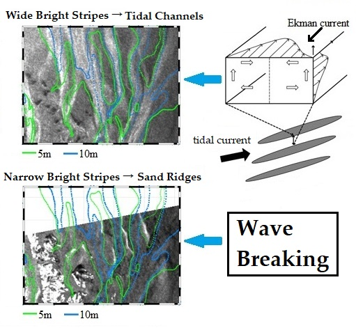
:In this study, the C-band radar backscatter features of the shallow water topography of Subei Bank in the Southern Yellow Sea are statistically investigated using 25 ENVISAT (Environmental Satellite) ASAR (advanced synthetic aperture radar) and ERS-2 (European Remote-Sensing Satellite-2) SAR images acquired between 2006 and 2010. Different bathymetric features are found on SAR imagery under different sea states. Under low to moderate wind speeds (3.1~6.3 m/s), the wide bright patterns with an average width of 6 km are shown and correspond to sea surface imprints of tidal channels formed by two adjacent sand ridges, while the sand ridges appear as narrower (only 1 km wide), fingerlike, quasi-linear features on SAR imagery in high winds (5.4~13.9 m/s). Two possible SAR imaging mechanisms of coastal bathymetry are proposed in the case where the flow is parallel to the major axes of tidal channels or sand ridges. When the surface Ekman current is opposite to the mean tidal flow, two vortexes will converge at the central line of the tidal channel in the upper layer and form a convergent zone over the sea surface. Thus, the tidal channels are shown as wide and bright stripes on SAR imagery. For the SAR imaging of sand ridges, all the SAR images were acquired at low tidal levels. In this case, the ocean surface waves are possibly broken up under strong winds when propagating from deep water to the shallower water, which leads to an increase of surface roughness over the sand ridges.

1. Introduction
A bathymetric measurement of shallow water is of fundamental importance to coastal environment research and resource management. The traditional bathymetric survey uses a shipboard sonar, single-beam, or multi-beam sounding system, which can provide high-precision data but is costly and inefficient. With the development of remote sensing techniques, the shallow water depth can be measured with high efficiency [1,2,3,4]. A spaceborne synthetic aperture radar (SAR), in particular, provides valuable information of shallow water topography in all-weather and day-night conditions with a high spatial resolution (a few to tens of meters). Although the SAR signal does not penetrate through sea water, the bathymetric features of shallow water (water depth < 50 m) or even deep water (water depth of about 600 m) can still be observed indirectly through the interaction between the ocean current and the underwater topography [5,6,7,8,9,10,11,12]. Shallow water bathymetric features were first discovered on radar images in 1969 [6,13]. Since then, many researchers have investigated the radar imaging mechanism of underwater topography in shallow waters. In 1984, Alpers and Hennings [7] developed a one-dimensional (1-D) SAR imaging model under the assumption that the current velocity is primarily normal to the direction of the major axis of topographic corrugation in the un-stratified ocean. The model was further enhanced by Van der Kooij et al. [14], Vogelzang et al. [15], and Romeiser and Alpers [16]. For a stratified ocean, Zheng et al. [8] obtained dynamical solutions for the vertical propagation of disturbance signals induced by underwater topography from the ocean bottom to the surface. All of these studies have shown that under the condition of a tidal current perpendicular to topographic features, the underwater topography can be imaged by SAR. However, recent satellite observations show that when the tidal current is parallel to topographic corrugations such as underwater sand ridges, sand bars, or tidal channels, the shallow water topography can also appear on SAR imagery [9,17,18,19]. These observations cannot be explained using the existing 1-D radar imaging model. Considering the tidal convergence, Li et al. [9] developed a two-dimensional (2-D) analytical model for the interpretation of SAR imaging of underwater sand ridges parallel to the tidal current. Recently, Zheng et al. [17] analyzed the secondary circulation induced by the flow parallel to the topographic corrugation by solving the three-dimensional (3-D) disturbance governing equations of the shear-flow. The theoretical results were applied to interpret SAR imaging of tidal channels. The above studies show that different bathymetric features might appear on SAR imagery. Then, under what dynamic conditions can shallow water bathymetry be observed by SAR in the case of the current being parallel to underwater topographic corrugations? Particularly, when will the sand ridges or tidal channels be shown on SAR imagery? The answers to these questions are still unclear.
With large amounts of sediment input from the river runoff, the radial sand ridges offshore from the middle Jiangsu coast in the Southern Yellow Sea (also called Subei Bank) were formed as a sediment physiognomy and represent an ideal region for harbor construction, agricultural development, and fishery production [20] (see Figure 1a). The distinguished characteristic of the topography in this area is the unique distribution of a group of tidal channels and shallow sand ridges radiating from Jianggang city [21] (see Figure 1b), which encompass an area larger than 200 km long and 140 km wide [22]. The major axes of the topographic corrugations are roughly parallel to the semidiurnal tidal currents.
In this study, the radar backscatter features of the shallow water topography of Subei Bank are investigated using ENVISAT (Environmental Satellite), ASAR (advanced synthetic aperture radar), and European Remote-Sensing Satellite-2 (ERS-2) SAR images. We analyze the influences of wind, current, and tide on the capability of C-band SAR in observing the underwater topography in this region, and try to find out the possible radar imaging mechanisms.
2. Data and Methods
The SAR data used in this study include 16 ENVISAT ASAR images and nine ERS-2 SAR images over Subei Bank in the Southern Yellow Sea acquired between 2006 and 2010. All these C-band SAR images are VV-polarized with a nominal spatial resolution of 30 30 m [23]. The ASAR system has been designed to provide continuity with ERS SAR by the European Space Agency (ESA). Compared with the ERS-1/2 SAR launched in 1991/1995, ASAR, launched in 2002, features extended observational capabilities, three new modes of operation, and improved performances [24]. Figure 2 presents examples of three typical types of SAR images over Subei Bank.
SAR not only observes oceanic or atmospheric phenomena, but also provides direct measurements of sea surface roughness that is related to sea surface wind speed (e.g., [25,26,27,28]). In this study, the sea surface wind speed (at 10-m height) is derived from SAR using the C-band geophysical model function CMOD5 [29] with wind direction interpolated from the six-hourly blended sea surface wind data from NOAA/National Climatic Data Center (NCDC). The NOAA/NCDC blended sea winds with a spatial resolution of 0.25° 0.25° are generated by blending observations from multiple satellites, which fills in the data gaps (in both time and space) of the individual satellite samplings and reduces the subsampling aliases and random errors [30].
In order to investigate the contribution of the tidal current and height to the SAR imaging of shallow water topography, we use the Tidal Model Driver (TMD) tide data to demonstrate the tide condition when SAR images were acquired. TMD is a package for accessing the harmonic constituents and making predictions of tidal height and currents [31,32]. As shown in Figure 3, compared with the data from two tide gauges and the Tide Table, the TMD results perform well in the tidal phase but present a systematic underestimation of tidal amplitude, which is possibly caused by the input of inaccurate water depth data in the tidal model in this region. By fitting the TMD results with in situ observations of the tidal height at Dongsha tide gauge in the lunar month of July 2014 (Figure 3a), we obtain a relationship between the observed tidal height (m) and the TMD output (m):
To validate the relationship, the TMD outputs of the tidal height in lunar August 2014, were corrected by Equation (1) and compared with in situ measurements from the same tide gauge (Figure 3b). One can see that the root mean square error (RMSE) between the TMD results and tide gauge observations is decreased significantly from 0.64 to 0.39 m after the correction. Similar results can be obtained for Liyashan tide gauge data collected in lunar September 2016, with the RMSE decreasing from 0.75 to 0.40 m (Figure 3c). Therefore, in the following study, the TMD output of the tidal height at SAR imaging time is corrected using Equation (1) for further analysis.
The bathymetry data of the whole study area are generated from the Sea Chart published by the China Navy Hydrographic Office in 2013 [33]. However, most Sea Chart data were measured in 1979. In addition, the data are relatively sparse and antiquated because of the evolution of sand ridges induced by the action of tidal current year after year [34]. For more accurate and higher-resolution water depth data, we carried out a field survey along the two cross sections A and B (Figure 1b) in December, 2016. The measured water depth data are used to interpret the bathymetric features of Subei Bank on SAR imagery.
3. Bathymetric Features of Subei Bank on SAR Imagery
From Figure 2, one can see the tidal channels or sand ridges are not always clearly shown on SAR imagery (see Figure 2a). Under certain sea states and wind conditions, the shallow water topography appears as fingerlike features (see Figure 2b,c). What is interesting is that distinct bathymetric features of the same region are shown on SAR images acquired at different times. In particular, an apparent difference occurs in the northeastern area (see the black boxes in Figure 2b,c). As shown in Figure 2b, there are some paralleled wide bright patterns in this region, and the average width of the stripes is about 6 km. However, the locations of the bright stripes change and are much narrower in Figure 2c with an average width of only 1 km.
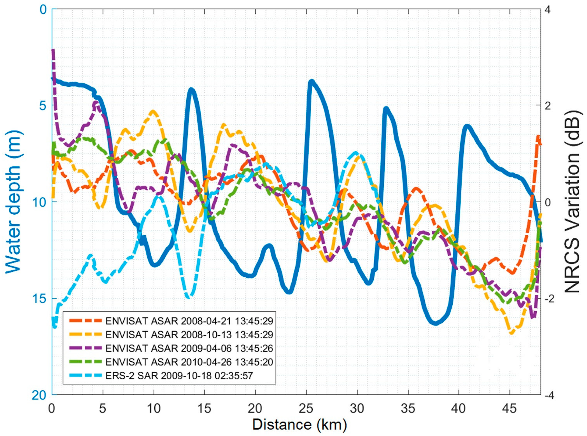
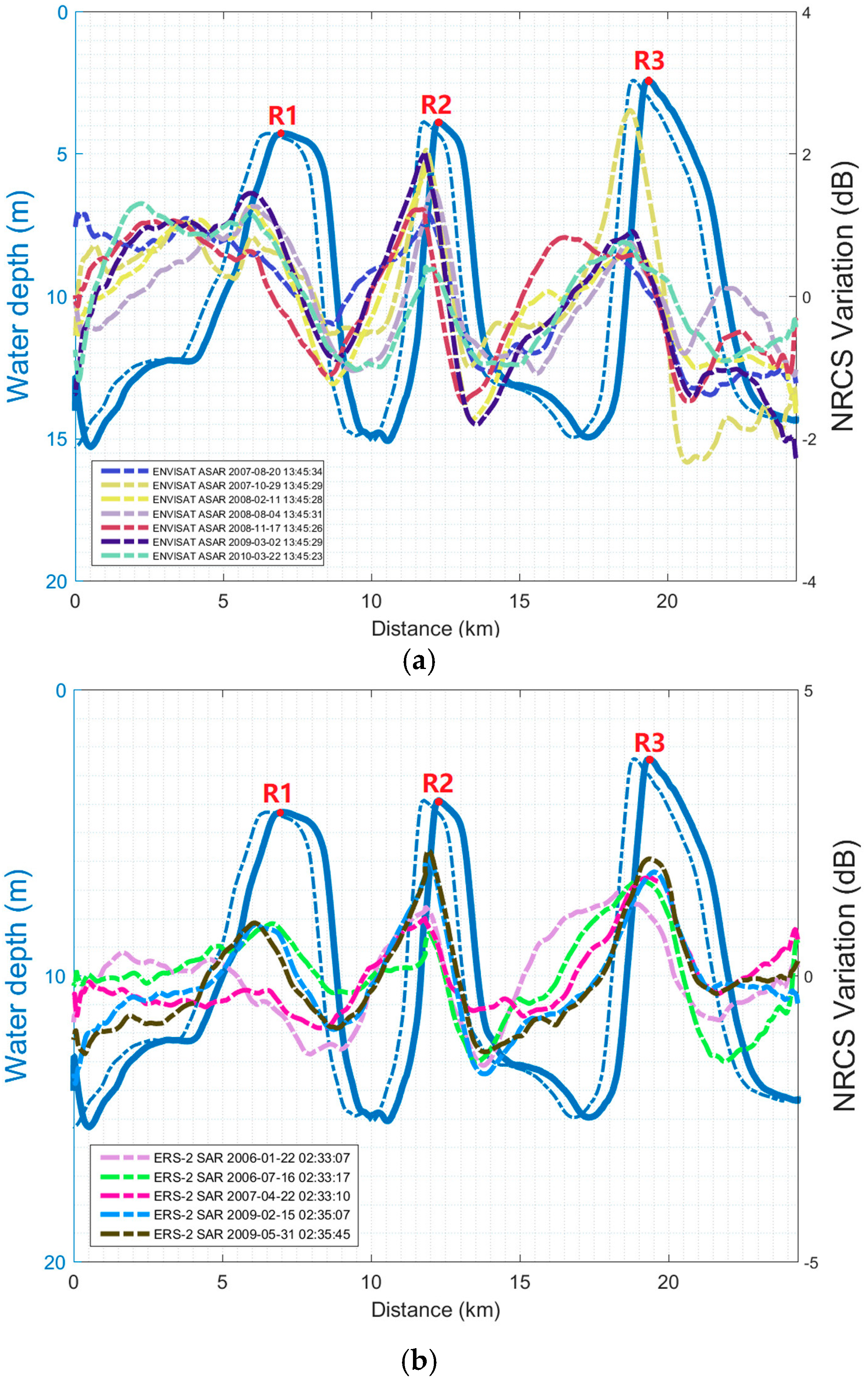
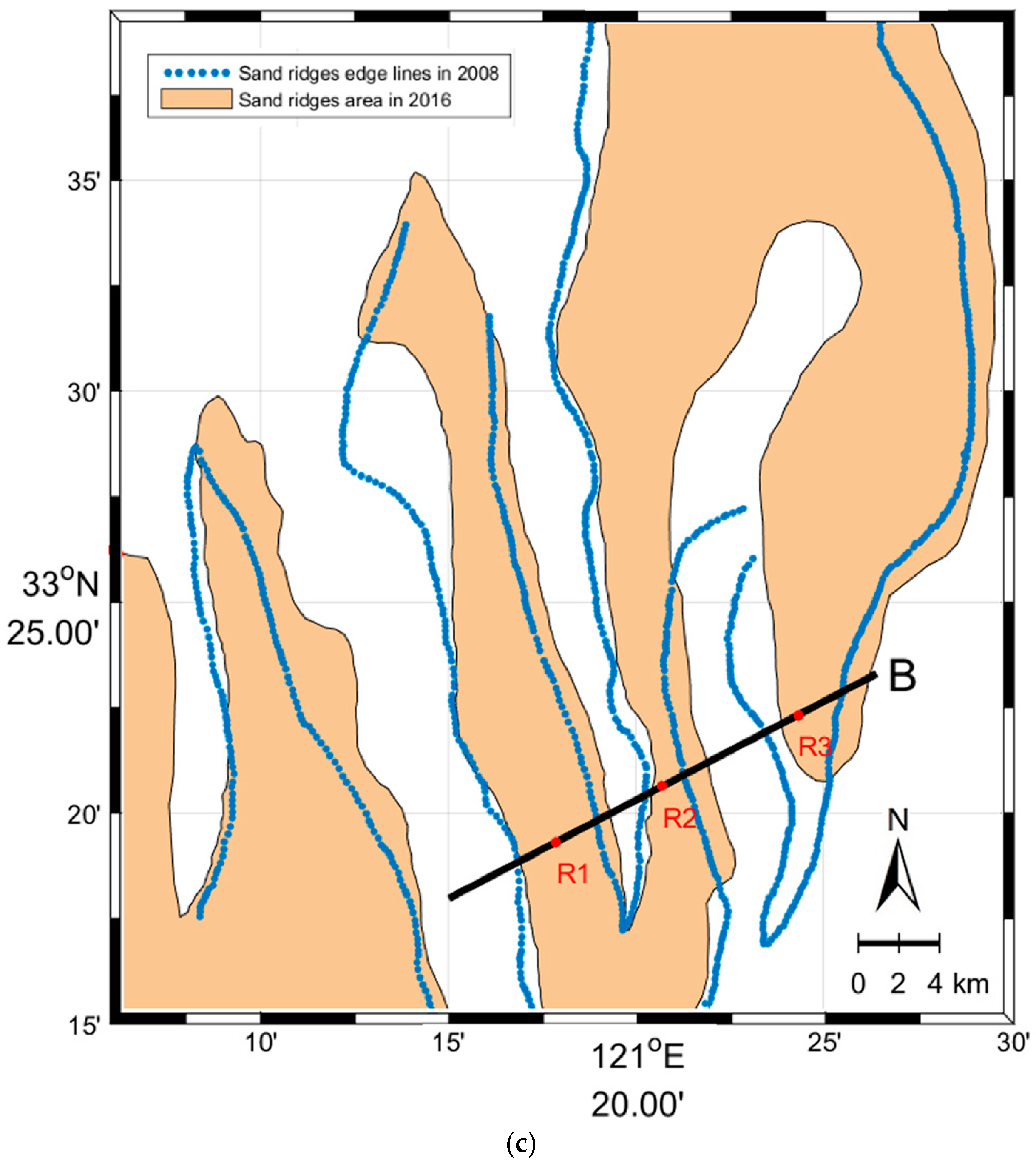
Among the 25 SAR images over Subei Bank, there are a total of eight SAR images without any bathymetric features (e.g., Figure 2a) and 17 images showing obvious bathymetric features. The paralleled wide bright patterns appear on five SAR images (Figure 4). By examining the Sea Chart bathymetric data, we find the locations of the wide bright stripes mainly coincide with the deep water area (>10 m) in this region. The relationship can be seen more clearly in Figure 5, which shows the variation of the SAR derived normalized radar backscatter cross section (NRCS) and water depth along the cross section A. Apparently, the wide bright stripes on this type of SAR image correspond to the deep water region, i.e., the tidal channels. The other 12 SAR images show obviously much narrower bright stripes at different locations (Figure 6). Comparing the variation of the NRCS with water depth along the cross section B (Figure 7), one can clearly see that these narrow bright stripes are sea surface imprints of underwater sand ridges. One may also notice that the SAR signal enhancement in Figure 7 does not take place exactly over the crest of the sand ridge measured in 2016, but with an offset of about 0.5 km westward (see the dashed blue line in Figure 7). The possible reason for this is that the topography of Subei Bank changes with time under the action of strong tidal currents [34]. To investigate the evolution of the sand ridges, we collect two optical images from Landsat_7 Enhanced Thematic Mapper Plus (ETM+) in 2008 (Figure 8a) and Landsat_8 Operational Land Imager (OLI) in 2016 (Figure 8b), respectively. The spatial resolution of the images is 30 m. Figure 8c shows the edge of the sand ridge in the study area extracted from the Landsat images. The deviation of the edge lines indicates that the sand ridges moved a little to the northeast from 2008 to 2016. This may partly explain why there is a small deviation between the locations of the peak of SAR observed NRCS and the crest of the sand ridge.
Table 1 shows ambient wind, current, and tide conditions at the acquisition time of 25 SAR images with or without obvious bathymetric features over Subei Bank. Most of the images with obvious underwater topographic features (13/17) were acquired during the flood tide, while most of those without any features (7/8) were acquired during the ebb tide. Comparing Figure 4 with Figure 6 and judging from the extent of the shoal exposed to the sea surface, we find that the water level at the time when the sand ridges were observed by SAR should be much lower than that when the tidal channels were imaged. This is further validated by the corrected TMD results. The values of the tidal heights when the SAR images with sand ridge features were acquired are all negative, and the water levels are below the mean sea level by over 1.3 m. For the images with tidal channel features, however, the tidal height is much larger and the water levels are all above the mean sea level. Another interesting thing to note is that the tidal channels were observed by SAR under low to moderate winds (3.1~6.3 m/s), while the sand ridges were detected at much higher wind speeds (5.4~13.9 m/s). This means that both the tidal height and wind may play a significant role in the SAR imaging of shallow water topography in this region.
4. SAR Imaging Mechanisms
Why does the underwater topography in the same region have distinctive radar backscatter features on SAR imagery? In this section, we discuss the possible imaging mechanisms of SAR imaging of shallow water topography over Subei Bank.
4.1. SAR Imaging of Tidal Channels
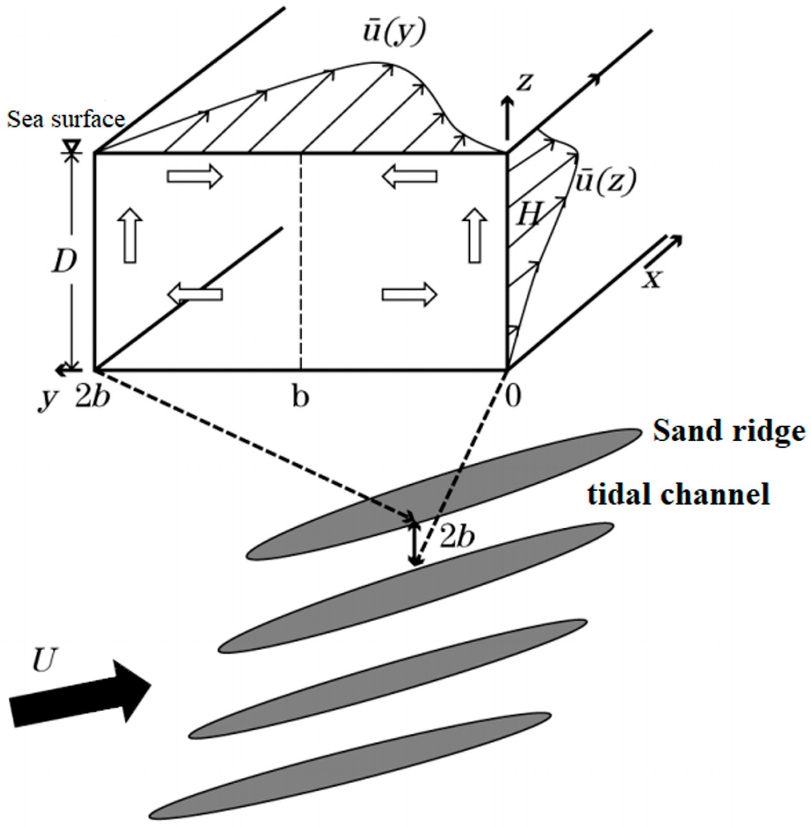
The existing SAR imaging theories of underwater topography are based on the following three processes: (1) the current and topography interaction generates sea surface current divergence or convergence zones; (2) the divergence and convergence of the current modulate the wind-generated sea surface wave spectrum; and (3) the variation of short surface wave height induces the backscatter variations seen in the SAR image [9]. Considering the sidewall friction, the surface, and the bottom Ekman layers, the authors proposed a physics model to analyze the secondary circulation induced by the flow parallel to underwater topographic corrugation (see Figure 9) [17]. The analytical solutions show that in the case where the direction of the surface Ekman current is opposite to the mean flow, there is a surface current convergent zone along the central line of a canal. Using this model, we tried to find the possible factors causing the sea surface imprints of tidal channels on SAR images over Subei Bank.
For the small area in this study, the wind and tidal current conditions over the tidal channels are nearly the same. Therefore, we can take one tidal channel as a representation to analyze the SAR imaging mechanism of the tidal channels. As sketched in Figure 9, we consider the flow in a long canal with a free surface and rectangular cross section with two flat sidewalls. The sidewalls have a height D and the bottom has a width 2b. A Cartesian coordinate system is set up with its origin located at the bottom. The vertical axis z is positive upward. The horizontal axis y is perpendicular to the central line and the vertical walls and positive leftward. The horizontal axis x is parallel to the walls and positive downstream. The 3-D scales of the canal, L1, L2 (=2b), and L3 (=D) satisfy L1 >> L2 >> L3. The mean flow (, , ) is driven by a pressure gradient externally imposed by a large-scale process, such as the tidal waves or the ocean circulation, and is thus considered a stable process. Due to the confinement of sidewalls, the mean flow is 1-D and parallel to the x-axis, i.e., (, ) = 0, and has horizontal and vertical velocity shears. The horizontal shear can be described by a parabolic profile as a plane Poiseuille flow [35]
where is the dynamic viscosity, and dP0/dx is the externally imposed pressure gradient. On the other hand, considering the existence of surface and bottom Ekman layers, we suppose that the vertical shear has a sinusoidal profile with an apex at H, as follows:
Thus, we have:
After solving the governing equations and taking some approximations (see Appendix A), we obtain the analytical solutions:
where .
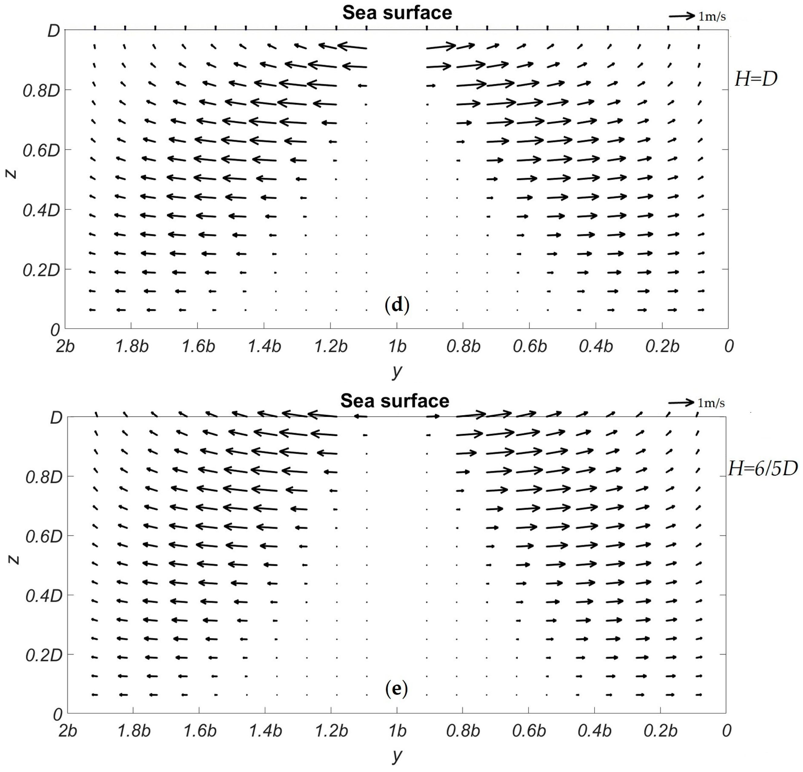
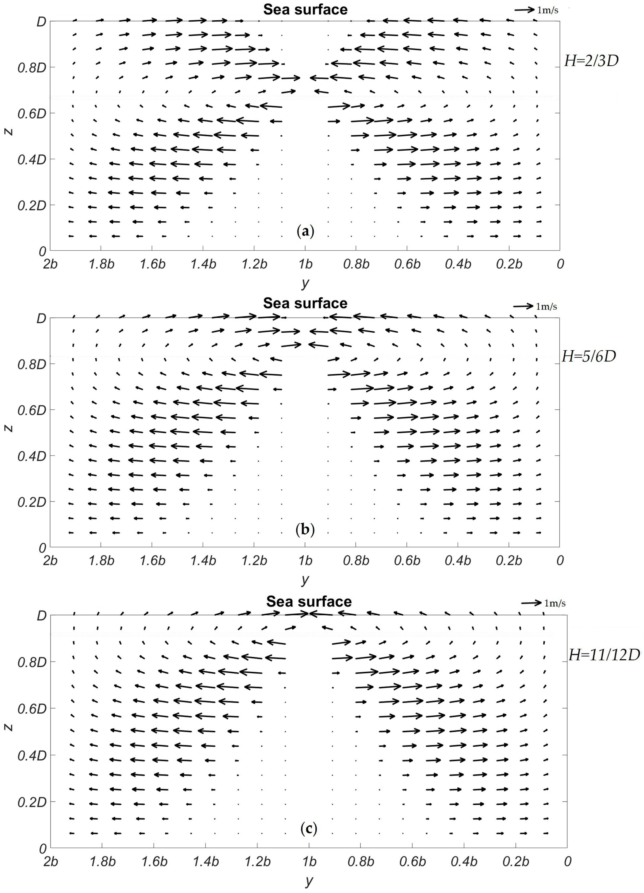
Solutions of Equations (5) and (6) are graphically shown in Figure 10. For the study area, we take D = 15 m, 2b = 6 km, and = 0.01 m/s. One can see the secondary circulation consists of a pair of current vortexes with opposite signs distributed symmetrically on the two sides of the central line of the channel, a cyclonic vortex on the right and an anti-cyclonic vortex on the left. The mean flow () shear drives upwelling along two sidewalls, and the stronger it is, the closer it is to the sidewalls. In the case of the presence of a surface Ekman layer where the direction of the Ekman current () component is opposite to that of the mean flow (H < D and ), the two vortexes converge at the central line of the canal in the upper layer. Thus, there is a surface current convergent zone along the central line of the canal. In addition, the convergence gets stronger with the increase of H in the case of H < D (see Figure 10a–c), which may imply that the strong tidal current and weak wind are favorable for the SAR imaging of the tidal channels. We also calculate the convergence value () at the sea surface when H = 5/6D. The value is about 10−3 s−1 and increases with the increase of H (H < D). Alpers (1985) [36] pointed out that 10−3 s−1 is the typical convergence value for the internal wave imaged by SAR, which is also sufficient to explain the bright stripes over the tidal channels on the SAR images in our study. In the case of the absence of a surface Ekman layer (H = D), there is no current convergent zone to be formed at any depth, as shown in Figure 10d. In the case of the presence of a surface Ekman layer with the direction identical to the mean flow (H > D, and ), the two vortexes diverge at the central line of the canal in all the layers, as shown in Figure 10e.
As shown in Table 1, all five SAR images with sea surface imprints of tidal channels in Subei Bank were acquired during flood tide, implying that the tidal current was mainly flowing southward and was parallel to the submerged sand ridges or tidal channels [37]. Meanwhile, according to the Ekman theory [38], the wind-driven surface Ekman current flows at an angle to the right of the prevailing wind direction. The wind direction of the five wide bright stripes images in Table 1 indicates that the Ekman velocity has a northward component. According to the physic model, when the tidal current and the surface Ekman current have opposite directions (), surface current convergence zones occur in the middle of two adjacent sand ridges, i.e., over the tidal channel region in this study. Therefore, the tidal channels appear as wide and bright stripes on the five SAR images.
4.2. SAR Imaging of Sand Ridges
For SAR imaging of underwater sand ridges, in most cases (nine out of 12), the secondary circulation theory is not applicable because the relationship between the tidal current and wind direction does not satisfy the necessary dynamic condition. However, as pointed out in the last section, the water levels at the imaging time are far below the mean sea level by over 1.3 m. In this case, the sea surface waves are most likely to break when propagating to shallower waters. Additionally, the ocean wave breaking has been proved to be one of the most frequent oceanic processes in Subei Bank [39]. In the following section, we will determine whether if this is true for the cases when sand ridges were observed by SAR.
The wave breaking generally occurs where the wave height reaches the point that the crest of the wave actually overturns [40]. Nelson and Gonsalvas [41] studied the laboratory and field wave data and developed a wave breaking relationship applicable to the regular and irregular waves:
where m is the sea floor slope, and is the ratio of the wave height () to wave breaking water depth (), i.e.,
Here, the wave breaking depth means that a wave will start to break when it reaches an area where the instantaneous water depth is smaller than .
For the fully developed ocean waves, the wave height can be expressed as [42]:
where is a non-dimensional constant taken to be 0.3, is the gravitational acceleration, and is the wind speed at 10 m from the sea surface.
The mean seafloor slope of the sand ridges in the study region (see Figure 7) is close to 0.004. Hence we have . Then, using Equations (8) and (9) and the SAR-derived wind speed, the wave height and the corresponding breaking depth at SAR imaging time are calculated and listed in Table 1. Considering the tidal height, all the instantaneous water depths at the sand ridge locations are smaller than the breaking depth, indicating that the surface waves under the relatively strong winds are quite likely to break when propagating over the extremely shallow sand ridges. The increase of surface roughness induced by breaking waves over the sand ridges will make the sea surface appear as narrow bright stripes on SAR imagery.
4.3. Discussion
Note that for some cases where the sand ridges are observed by SAR (cases 6, 7, and 12), or topographic features are not shown on SAR imagery (cases 19, 21, 22, and 25), the tidal current was also opposite to the wind direction. According to the secondary circulation theory proposed above, the tidal channels might also be observed by SAR in these cases. However, the wide bright stripes corresponding to the tidal channels are not shown on these images. Why? If we look at the wind and current conditions in more detail, we find the images were all acquired under high winds (6.1~10.5 m/s), implying relatively high NRCS values throughout the study area. On the other hand, as the output from the TMD model shows, the time differences between the acquisition times of these SAR images and the local high or low tide times are within 1.5 h, indicating that the tidal current velocity might be so weak (and even close to 0) that the convergence does not occur at the surface over the tidal channels, or the signal enhancement generated by the weak convergence is not strong enough to be observed by SAR compared to the ambient high NRCS induced by the winds.
From Figure 7, one can see that the peak NRCS positions exhibit very little movement. One possible reason for this is that the topography of Subei Bank changes slowly with time under the action of strong tidal currents and this change may fluctuate if the sea state changes severely (e.g., typhoon, storm current, etc.) in some years [34,37]. From another perspective, we may be able to use SAR to observe the short-term change and long-term evolution of the sand ridges. For some few cases under a relatively high wind speed where the instantaneous water depth is smaller than the wave breaking depth, since the slope of the sand ridge in the study area is very steep, the relatively strong wind also impelled the breaking wave to quickly propagate to the peak of the sand ridges. Therefore, the breaking wave induced increase in surface roughness is larger over the shallower sand ridge and is observed by SAR.
5. Conclusions
In this study, 25 ENVISAT ASAR and ERS-2 SAR images are analyzed to investigate the C-band radar backscatter features of the shallow water topography over Subei Bank in the Southern Yellow Sea of China, where the flow is primarily parallel to the major axes of tidal channels or sand ridges. Based on the statistical analysis, we find the bathymetric features are not always shown on SAR imagery. For SAR images with obvious topographic features, paralleled fingerlike bright stripes appear at different locations and have distinct widths. The tidal channels appear as wide bright stripes with an average width of 6 km on SAR images under low to moderate wind speeds, while the sea surface imprints of underwater sand ridges on SAR imagery are narrow (~1 km wide), quasi-linear, bright stripes at high winds.
Theoretical analysis suggests that the reason why tidal channels are observed by C-band SAR under low to moderate winds is that the tidal current and the wind-driven surface Ekman current have opposite directions. In this case, a convergent zone at the sea surface forms at the central line of the tidal channel due to the convergence of two vortexes in the upper layer. Therefore, the tidal channels are shown as relatively wide bright stripes on SAR imagery. However, the tidal channels might not be able to be detected by SAR at high winds due to the high NRCS value of background seawaters, even if the above dynamic condition is fulfilled. For SAR imaging of the sand ridges in the study area, both the low water level and strong winds provide favorable conditions for the breaking of ocean surface waves when propagating to the shallow waters, thus leading to an increase of SAR observed NRCS over the shallow sand ridges.
Acknowledgments
The ENVISAT ASAR data used in this study were provided by the Institute of Space and Earth Information Science of the Chinese University of Hong Kong. The ERS-2 SAR data are from the ESA and the Open Spatial Data Sharing Project of Institute of Remote Sensing and Digital Earth Chinese Academy. This work was supported by the National Key Project of Research and Development Plan of China (Grant No. 2016YFC1401905), the Fundamental Research Funds for the Central Universities (Hohai University) (Grants No. 2015B15914 and 2017B714X14), the Postgraduate Research & Practice Innovation Program of Jiangsu Province (Grant No. KYCX17_0507), and the project of the Priority Academic Program Development of Jiangsu Higher Education Institutions (Ocean Science). The views, opinions, and findings contained in this report are those of the authors and should not be construed as an official NOAA or U.S. Government position, policy, or decision.
Author Contributions
Qing Xu and Shuangshang Zhang initiated the research. Under the supervision of Qing Xu, Quanan Zheng and Xiaofeng Li, Shuangshang Zhang performed the experiments and analysis. Shuangshang Zhang and Qing Xu drafted the manuscript. Quanan Zheng and Xiaofeng Li revised the paper. All authors read and approved the final version of the manuscript.
Conflicts of Interest
The authors declare no conflict of interest.
Appendix A. Derivation of Secondary Circulation Solutions
Consider the governing equations for a flow consisting of mean flow and disturbance:
where is the Coriolis parameter; is the pressure; is the water density; is the kinetic viscosity; , , and are the components of external forcing; g is the gravitational acceleration; and:
The boundary conditions are:
and
Substituting (A5) into (A1)–(A4) yields the disturbance governing equations:
The boundary conditions are:
and
In order to examine the role of velocity shear in generating the secondary circulation, we further take the following approximations: (1) ignoring the viscous terms; (2) assuming the x-coordinate scale of mean flow , , is much larger than that of the disturbance, L, thus resulting in ; (3) the x-coordinate scale of disturbance is much larger than that of the y-coordinate scale, thus resulting in ; (4) in Equations (A8)–(A10), the velocity shear terms are much larger than other terms. Thus, we have the simplified disturbance equations:
From (A15) and (A16), we have:
i.e., and are independent of x. From (A14) and (A17), we derive a secondary circulation equation of :
where is defined as
Equation (A19) has an analytical solution of
where is a constant to be determined. From (A14) we have:
where .
References
- He, X.; Chen, N.; Zhang, H.; Fu, B.; Wang, X. Reconstruction of sand wave bathymetry using both satellite imagery and multi-beam bathymetric data: A case study of the Taiwan Banks. Int. J. Remote Sens. 2014, 35, 3286–3299. [Google Scholar] [CrossRef]
- Ma, S.; Tao, Z.; Yang, X.; Yu, Y.; Zhou, X.; Li, Z. Bathymetry retrieval from hyperspectral remote sensing data in optical-shallow water. IEEE Trans. Geosci. Remote Sens. 2014, 52, 1205–1212. [Google Scholar] [CrossRef]
- Pacheco, A.; Horta, J.; Loureiro, C.; Ferreira, Ó. Retrieval of nearshore bathymetry from Landsat 8 images: A tool for coastal monitoring in shallow waters. Remote Sens. Environ. 2015, 159, 102–116. [Google Scholar] [CrossRef]
- Wozencraft, J.M.; Millar, D. Airborne LIDAR and integrated technologies for coastal mapping and nautical charting. Mar. Technol. Soc. J. 2005, 39, 27–35. [Google Scholar] [CrossRef]
- Shi, W.; Wang, M.; Li, X.; Pichel, W.G. Ocean sand ridge signatures in the Bohai Sea observed by satellite ocean color and synthetic aperture radar measurements. Remote Sens. Environ. 2011, 115, 1926–1934. [Google Scholar] [CrossRef]
- De Loor, G.P. The observation of tidal patterns, currents, and bathymetry with SLAR imagery of the sea. IEEE J. Ocean. Eng. 1981, 6, 124–129. [Google Scholar] [CrossRef]
- Alpers, W.; Hennings, I. A theory of the imaging mechanism of underwater bottom topography by real and synthetic aperture radar. J. Geophys. Res. 1984, 89, 1029–1054. [Google Scholar] [CrossRef]
- Zheng, Q.; Li, L.; Guo, X.; Ge, Y.; Zhu, D.; Li, C. SAR Imaging and hydrodynamic analysis of ocean bottom topographic waves. J. Geophys. Res. 2006, 111. [Google Scholar] [CrossRef]
- Li, X.; Li, C.; Xu, Q.; Pichel, W.G. Sea surface manifestation of along-tidal-channel underwater ridges imaged by SAR. IEEE Trans. Geosci. Remote Sens. 2009, 47, 2467–2477. [Google Scholar] [CrossRef]
- Li, X.; Yang, X.; Zheng, Q.; Pietrafesa, L.J.; Pichel, W.G.; Li, Z.; Li, X. Deep-water bathymetry feature imaged by spaceborne SAR in the Gulf Stream region. Geophys. Res. Lett. 2010, 37. [Google Scholar] [CrossRef]
- Hennings, I. An historical overview of radar imagery of sea bottom topography. Int. J. Remote Sens. 1998, 19, 1447–1454. [Google Scholar] [CrossRef]
- Zheng, Q.; Holt, B.; Li, X.; Liu, X.; Zhao, Q.; Yuan, Y.; Yang, X. Deep-water seamount wakes on SEASAT SAR image in the Gulf Stream region. Geophys. Res. Lett. 2012, 39. [Google Scholar] [CrossRef]
- De Loor, G.P.; Hulten, B.V. Microwave Measurements over the North Sea. Bound. Layer Meteorol. 1978, 13, 119–131. [Google Scholar] [CrossRef]
- Van der Kooij, M.W.A.; Vogelzang, J.; Calkoen, C.J. A simple analytical model for brightness modulations caused by submarine sand waves in radar imagery. J. Geophys. Res. 1995, 100, 7069–7082. [Google Scholar] [CrossRef]
- Vogelzang, J.; Wensink, G.J.; Calkoen, C.J.; Van der Kooij, M.W.A. Mapping Submarine Sand Waves with Multiband Imaging Radar: Experimental Results and Model Comparison. J. Geophys. Res. 1997, 102, 1183–1192. [Google Scholar] [CrossRef]
- Romeiser, R.; Alpers, W. An improved composite surface model for the radar backscattering cross section of the ocean surface, 2, Model response to surface roughness variations and the radar imaging of underwater bottom topography. J. Geophys. Res. 1997, 102, 25251–25267. [Google Scholar] [CrossRef]
- Zheng, Q.; Zhao, Q.; Yuan, Y.; Xian, L.; Hu, J.; Liu, X.; Yin, L.; Ye, Y. Shear-flow induced secondary circulation in parallel underwater topographic corrugation and its application to satellite image interpretation. J. Ocean. Univ. China 2012, 11, 427–435. [Google Scholar] [CrossRef]
- Wang, X.; Zhang, H.; Li, X.; Fu, B.; Guan, W. SAR imaging of a topography-induced current front in a tidal channel. Int. J. Remote Sens. 2015, 36, 3563–3574. [Google Scholar] [CrossRef]
- Zhang, S.; Xu, Q.; Cheng, Y.; Li, Y.; Huang, Q. Bathymetric features of Subei Bank on ENVISAT ASAR images. In Proceedings of the IEEE Progress in Electromagnetic Research Symposium (PIERS), Shanghai, China, 8–11 August 2016. [Google Scholar]
- Liu, Y.; Li, M.; Cheng, L.; Li, F.; Chen, K. Topographic mapping of offshore sandbank tidal flats using the waterline detection method: A case study on the Dongsha Sandbank of Jiangsu Radial Tidal Sand Ridges, China. Mar. Geod. 2012, 35, 362–378. [Google Scholar] [CrossRef]
- Iwenfei, N.; Wang, Y.; Zou, X.; Zhang, J.; Gao, J. Sediment dynamics in an offshore tidal channel in the southern Yellow Sea. Int. J. Remote Sens. 2014, 29, 246–259. [Google Scholar] [CrossRef]
- Song, Y.; Zhang, J. Study on Evolutions of Jiangsu Radiating Sandbanks Based on SAR Images. In Advances in SAR Oceanography from Envisat and ERS Missions, Proceedings of the SEASAR 2006, Frascati, Italy, 23–26 January 2006; Lacoste, H., Ouwehand, L., Eds.; ESA Publications Division: Noordwijk, The Netherlands, 2006; Available online: https://earth.esa.int/workshops/seasar2006/proceedings/papers/p11_song.pdf (accessed on 1 November 2017).
- Desnos, Y.L.; Buck, C.; Guijarro, J.; Suchail, J.L.; Torres, R.; Attema, E. ASAR-ENVISAT’s advanced synthetic aperture radar. ESA Bull. 2000, 102, 91–100. [Google Scholar]
- Moreira, A.; Prats-Iraola, P.; Younis, M.; Krieger, G.; Hajnsek, I.; Papathanassiou, K.P. A tutorial on synthetic aperture radar. IEEE Geosci. Remote Sens. Mag. 2013, 1, 6–43. [Google Scholar] [CrossRef] [Green Version]
- Lin, H.; Xu, Q.; Zheng, Q. An overview on SAR measurements of sea surface wind. Prog. Nat. Sci. 2008, 18, 913–919. [Google Scholar] [CrossRef]
- Xu, Q.; Lin, H.; Li, X.; Zuo, J.; Zheng, Q.; Pichel, W.G.; Liu, Y. Assessment of an analytical model for sea surface wind speed retrieval from spaceborne SAR. Int. J. Remote Sens. 2010, 31, 993–1008. [Google Scholar] [CrossRef]
- Yang, X.; Li, X.; Zheng, Q.; Gu, X.; Pichel, W.G.; Li, Z. Comparison of ocean surface winds retrieved from QuikSCAT scatterometer and Radarsat-1 SAR in offshore waters of the U.S. West Coast. IEEE Geosci. Remote Sens. Lett. 2010, 8, 163–167. [Google Scholar] [CrossRef]
- Yang, X.; Li, X.; Pichel, W.G.; Li, Z. Comparison of ocean surface winds from ENVISAT ASAR, MetOp ASCAT scatterometer, buoy measurements, and NOGAPS model. IEEE Trans. Geosci. Remote Sens. 2011, 49, 4743–4750. [Google Scholar] [CrossRef]
- Hersbach, H.; Stoffelen, A.; De, S.H. An improved c-band scatterometer ocean geophysical model function: CMOD5. J. Geophys. Res. 2007, 112, 225–237. [Google Scholar] [CrossRef]
- Zhang, H.; Bates, J.J.; Reynolds, R.W. Assessment of composite global sampling: Sea surface wind speed. Geophys. Res. Lett. 2006, 33, L17714. [Google Scholar] [CrossRef]
- Egbert, G.D.; Erofeeva, S.Y. Efficient inverse modeling of barotropic ocean tides. J. Atmos. Ocean. Technol. 2002, 19, 183–204. [Google Scholar] [CrossRef]
- Padman, L.; Erofeeva, S. Tide Model Driver (TMD) Manual; Earth & Space Research: Seattle, WA, USA, 2005. [Google Scholar]
- The Navigation Guarantee Department of the Chinese Navy Headquarters. Sea Chart of Yellow Sea: Sheyanghe Kou to Lvsi Gang; China Navigation Publications Press: Tianjin, China, 2013. [Google Scholar]
- Chen, J.; Wang, Y.; Zhang, R.; Lin, X. Stability study on the Dongsha Sandbanks in submarine radial sand ridges field off Jiangsu coast. Ocean Eng. 2007, 25, 105–113. [Google Scholar]
- Kundu, P.K. Fluid Mechanics; Academic Press: New York, NY, USA, 1990; pp. 263–298. [Google Scholar]
- Alpers, W. Theory of radar imaging of internal waves. Nature 1985, 314, 245–247. [Google Scholar] [CrossRef]
- Zhang, C.; Zhang, D.; Zhang, J.; Wang, Z. Tidal current-induced formation—Storm-induced change—Tidal current-induced recovery. Sci. China Ser. D Earth Sci. 1999, 42, 1–12. [Google Scholar] [CrossRef]
- Ekman, V.W. On the influence of the earth’s rotation on ocean currents. Matem. Astr. Fysik. 1905, 2, 1–52. [Google Scholar]
- Yang, Y.; Feng, W. Numerical simulation of wave fields in radial sand ridge filed of southern yellow sea. J. Hohai Univ. 2010, 38, 457–461. [Google Scholar]
- Evander, L. Breaking Wave; Alphascript Publishing: Beau Bassin, Mauritius, 2010. [Google Scholar]
- Nelson, R.C.; Gonsalves, J. Surf zone transformation of wave height to water depth ratios. Coast. Eng. 1992, 17, 49–70. [Google Scholar] [CrossRef]
- Hubert, W.E. A preliminary report on numerical sea condition forecasts. Mon. Weather Rev. 1957, 85, 200–204. [Google Scholar] [CrossRef]
Figure 1.
(a) Bathymetry (m) of the Yellow Sea and (b) Subei Bank boarded by dashed lines in panel (a). The bathymetry data are from ETOPO2 (National Centers for Environmental Information, 2006) for (a) and Sea Chart (published by China Navy Hydrographic Office, 2013) for (b). The cross sections A and B in (b) (black lines) are primarily perpendicular to the paralleled bright stripes on SAR imagery in Figure 2. The black dots denote the locations of the Dongsha and Liyashan tide gauges.
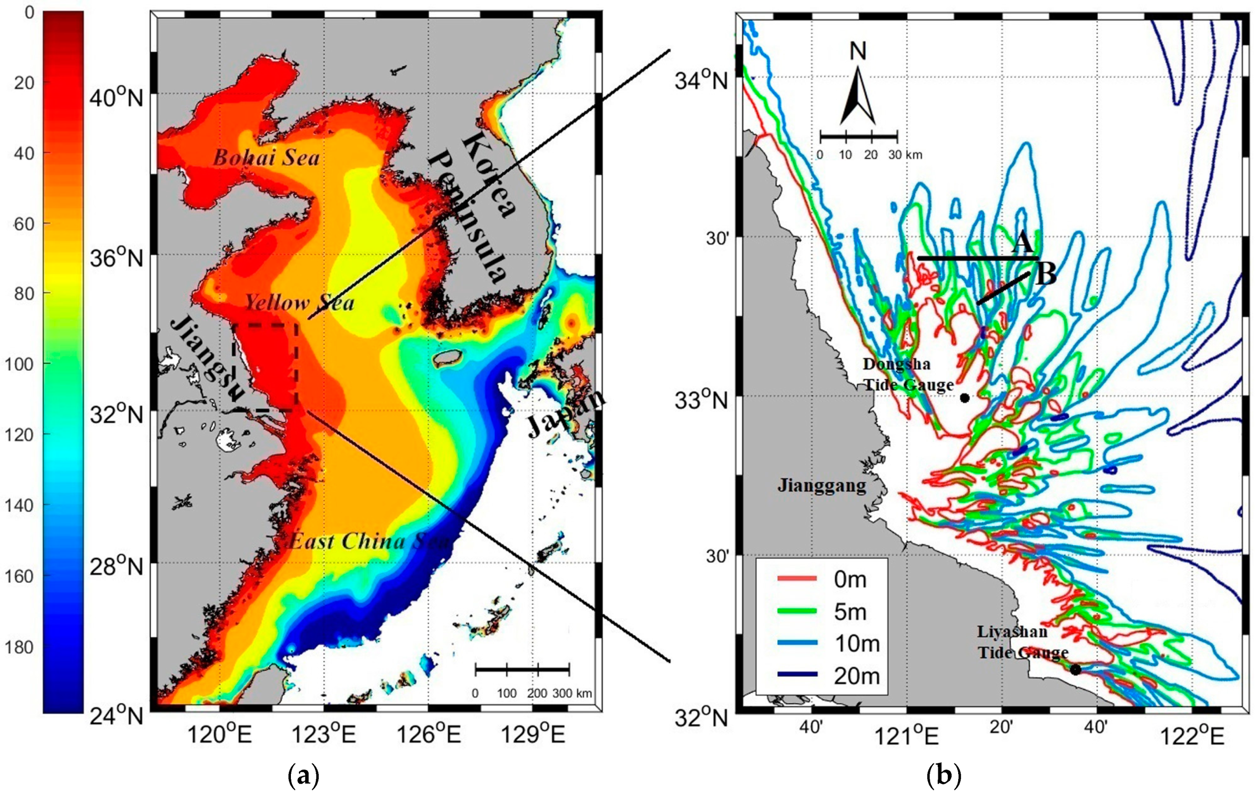
Figure 2.
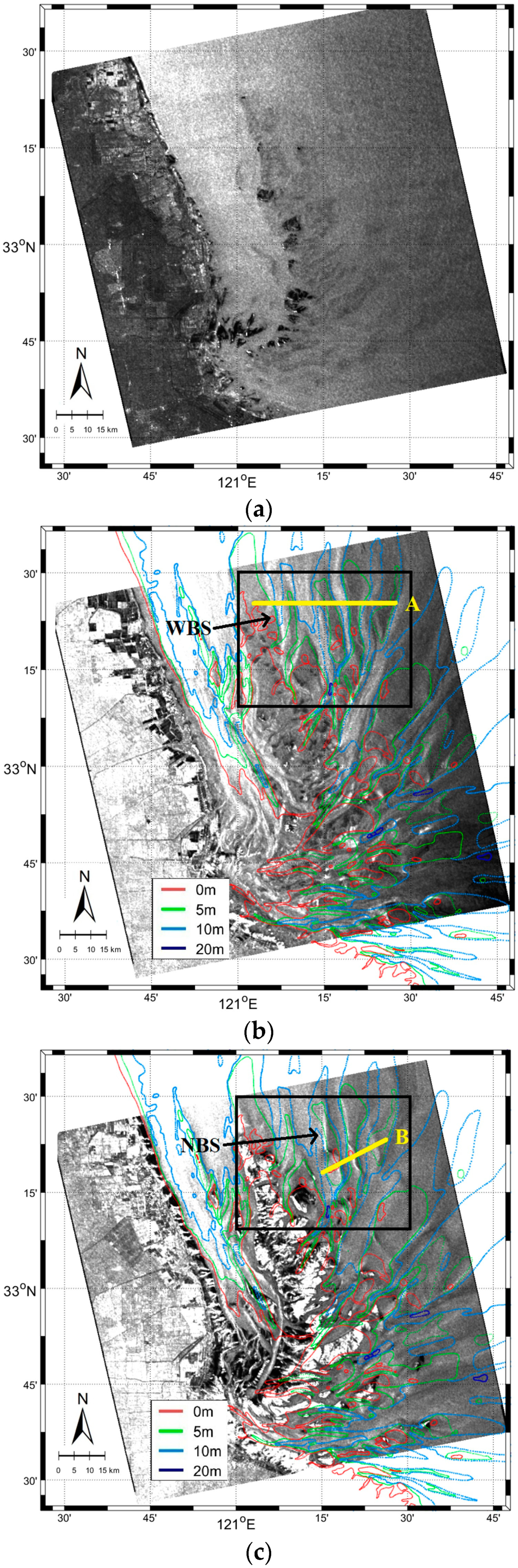
Examples of three typical ENVISAT ASAR images over Subei Bank: (a) image without any bathymetric features acquired at 13:45:32 UTC on 22 December 2008; (b) image with bathymetric features shown as wide bright stripes (WBS) in the small region denoted by the black rectangle, acquired at 13:45:29 UTC on 13 October 2008; (c) image with bathymetric features shown as narrow bright stripes (NBS) in the same region as (b), acquired at 13:45:28 UTC on 11 February 2008. The contours are water depth (m). The cross sections A and B (yellow lines, also shown as black lines in Figure 1b) are perpendicular to the paralleled bright stripes on SAR images.
Figure 2.
Examples of three typical ENVISAT ASAR images over Subei Bank: (a) image without any bathymetric features acquired at 13:45:32 UTC on 22 December 2008; (b) image with bathymetric features shown as wide bright stripes (WBS) in the small region denoted by the black rectangle, acquired at 13:45:29 UTC on 13 October 2008; (c) image with bathymetric features shown as narrow bright stripes (NBS) in the same region as (b), acquired at 13:45:28 UTC on 11 February 2008. The contours are water depth (m). The cross sections A and B (yellow lines, also shown as black lines in Figure 1b) are perpendicular to the paralleled bright stripes on SAR images.

Figure 3.
Comparison of the TMD results of the tidal height with in situ observations in lunar July (a) and August (b), 2014 at Dongsha tide gauge, and lunar September, 2016 at Liyashan tide gauge (c).
Figure 3.
Comparison of the TMD results of the tidal height with in situ observations in lunar July (a) and August (b), 2014 at Dongsha tide gauge, and lunar September, 2016 at Liyashan tide gauge (c).
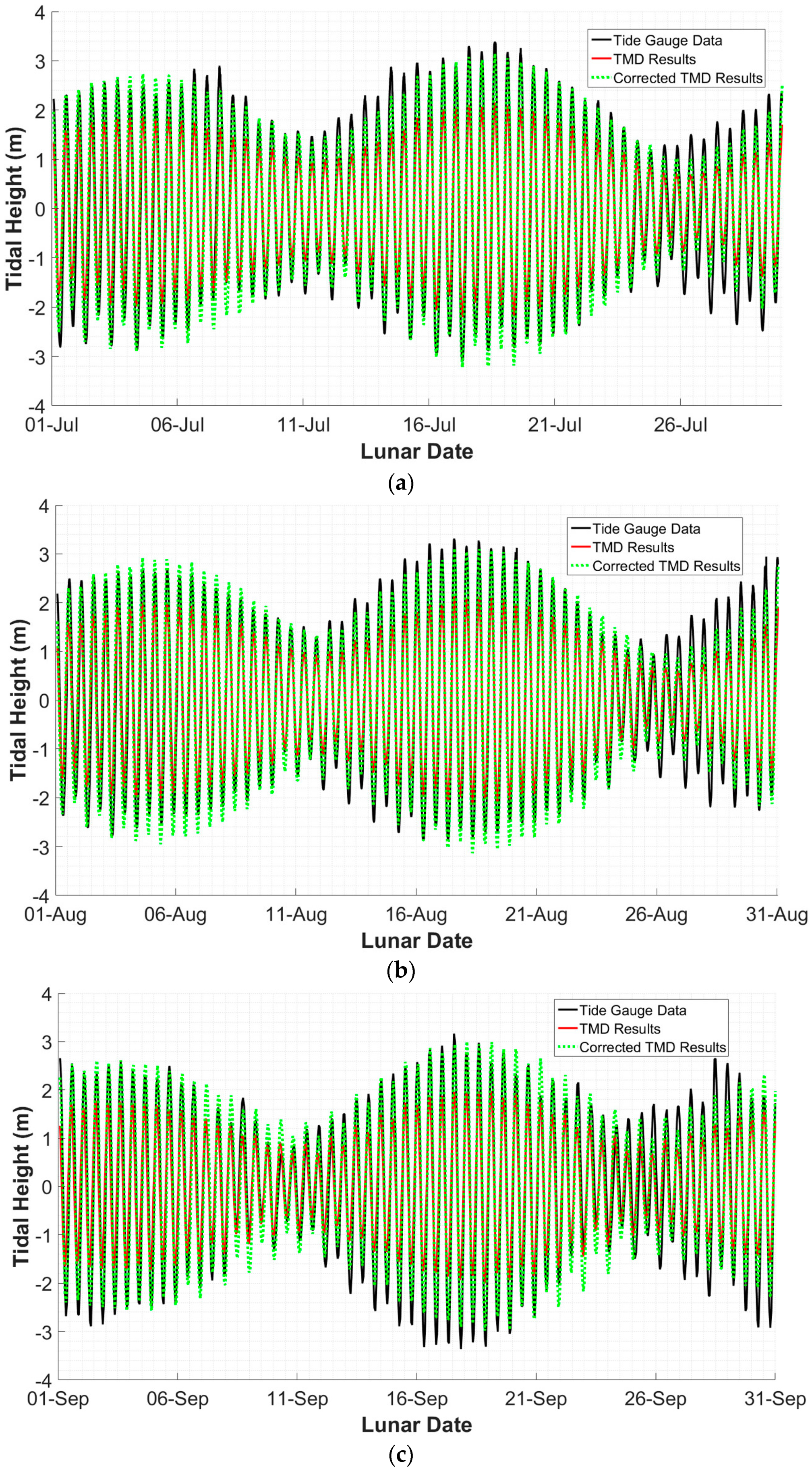
Figure 4.
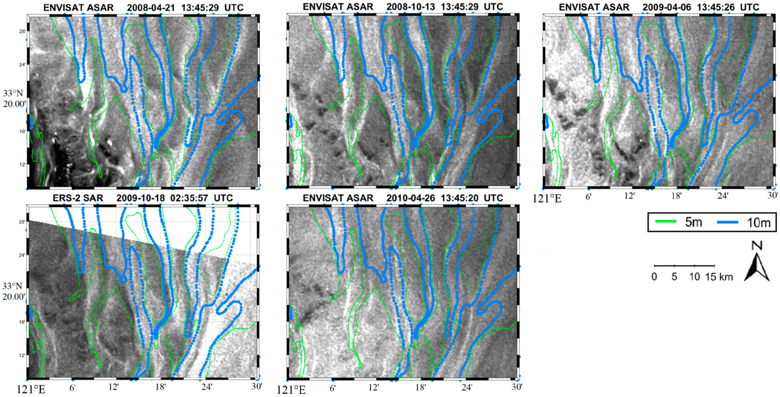
SAR sub-images over Subei Bank with bathymetric features shown as wide bright stripes. Green and blue lines are water depth contours of 5 and 10 m, respectively.
Figure 4.
SAR sub-images over Subei Bank with bathymetric features shown as wide bright stripes. Green and blue lines are water depth contours of 5 and 10 m, respectively.

Figure 5.
The water depth measured in December, 2016 (m) in blue solid line and NRCS Variation (dB) calculated from SAR data along the cross section A. The distance is measured from the left to the right for each cross section.
Figure 5.
The water depth measured in December, 2016 (m) in blue solid line and NRCS Variation (dB) calculated from SAR data along the cross section A. The distance is measured from the left to the right for each cross section.

Figure 6.
Same as Figure 4 but for SAR sub-images with bathymetric features shown as narrow bright stripes.
Figure 6.
Same as Figure 4 but for SAR sub-images with bathymetric features shown as narrow bright stripes.
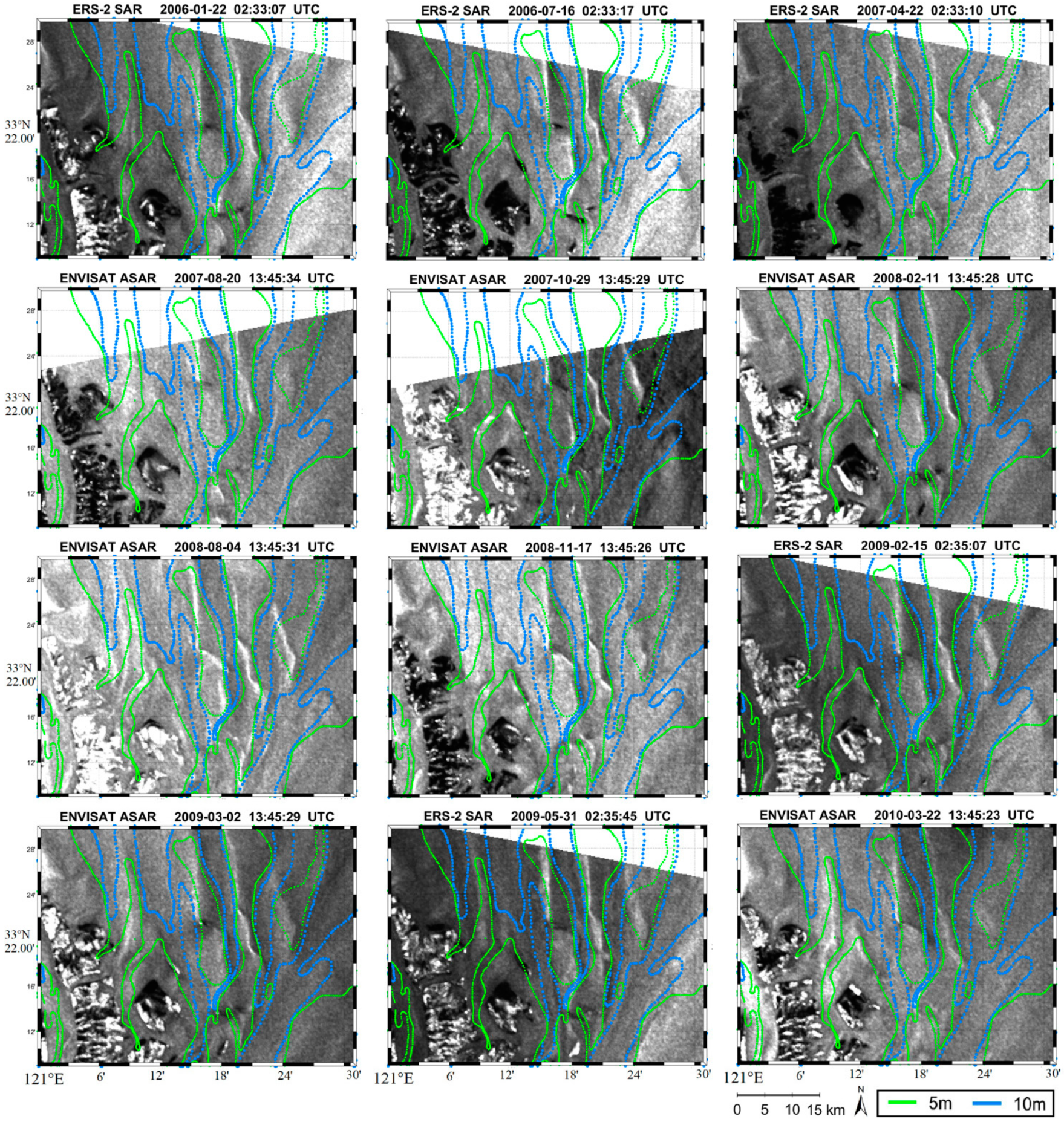
Figure 7.
Same as Figure 5 but along the cross section B: (a) for ENVISAT ASAR images and (b) for ERS-2 SAR images. The locations of the crests of the three sand ridges along cross section B are marked as R1, R2, and R3, respectively. The blue dashed line is the same as the blue solid line but has a deviation of 0.5 km westward.

Figure 8.
Landsat images over Subei Bank: (a) Landsat_7 ETM+ image acquired at 02:20:53 UTC on 24 April 2008; (b) Landsat_8 OLI image acquired at 02:30:41 UTC on 18 February 2016; and (c) the edge of the sand ridges in the study area (yellow dashed box in (a,b)) extracted from Landsat images. The dotted blue line denotes the edge extracted from (a) in 2008, and the light brown patch denotes the sand ridge area extracted from (b) in 2016. The field survey along cross section B is the same as that in Figure 1b with R1, R2, and R3 representing the locations of the sand ridge crests measured in 2016.
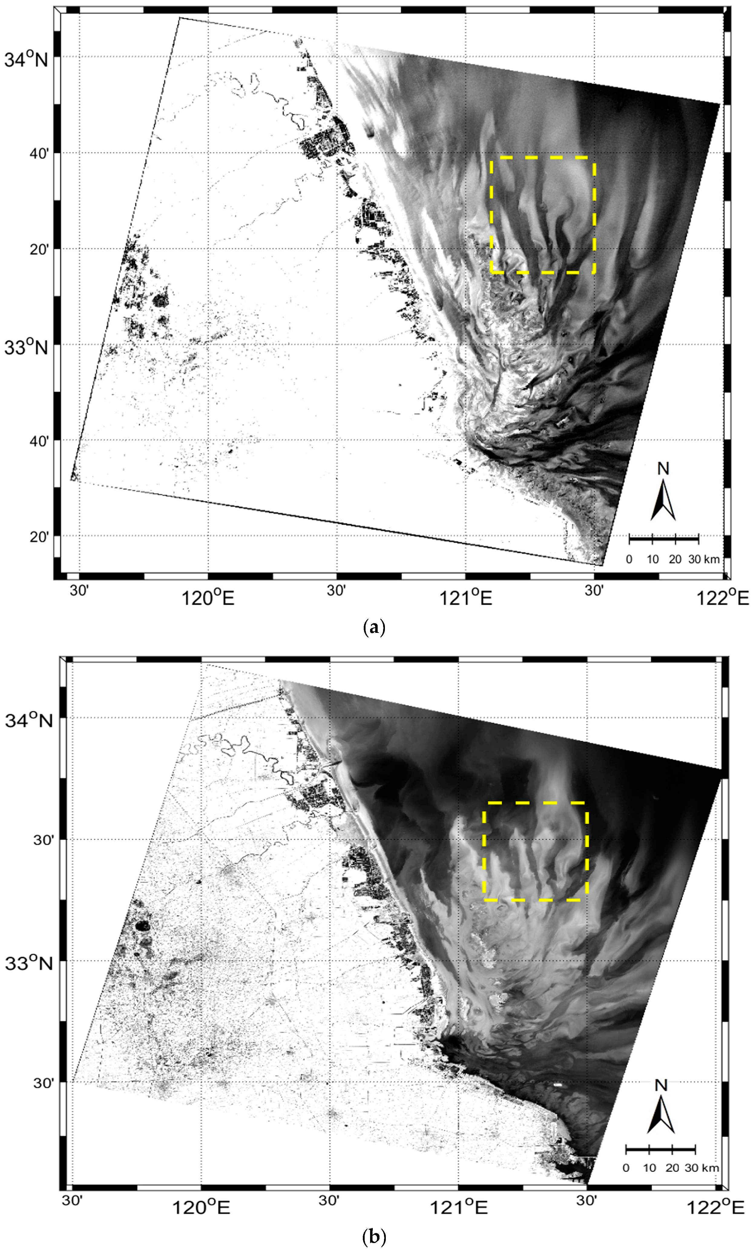

Figure 9.
The physics model for secondary circulation (large hollow arrows) induced by a shear flow over parallel underwater topographic corrugation.
Figure 9.
The physics model for secondary circulation (large hollow arrows) induced by a shear flow over parallel underwater topographic corrugation.

Figure 10.
Analytical solutions of the secondary circulation induced by a shear flow in a long, rectangular canal. (a) There is an upper Ekman layer, in which the Ekman current has a negative component in the mean flow direction () and H = 2/3D; (b) The same as (a) but for H = 5/6D; (c) The same as (a) but for H = 11/12D; (d) No upper Ekman layer; (e) There is an upper Ekman layer, in which the Ekman current has a positive component in the mean flow direction (). The vertical velocity is 10 times larger for plotting the solutions.


Table 1.
Wind, current, and tide conditions at an imaging time of 25 SAR images.
| Satellite | Date | Bathymetric Features 1 | Tidal Phase | Wind Direction 2 | Tidal Height (m) | Wind Speed (m/s) | Wave Height (m) | Wave Breaking Depth (m) | Instantaneous Water Depth (m) | |
|---|---|---|---|---|---|---|---|---|---|---|
| 1 | ENVISAT | 2008-04-21 | WBS | flood | 105 | 0.29 | 6.30 | 1.22 | 1.90 | 4.61 |
| 2 | ENVISAT | 2008-10-13 | WBS | flood | 174 | 1.61 | 4.80 | 0.71 | 1.10 | 5.93 |
| 3 | ENVISAT | 2009-04-06 | WBS | flood | 172 | 1.83 | 3.10 | 0.29 | 0.46 | 6.15 |
| 4 | ERS-2 | 2009-10-18 | WBS | flood | 195 | 1.90 | 5.60 | 0.96 | 1.50 | 6.22 |
| 5 | ENVISAT | 2010-04-26 | WBS | flood | 210 | 1.76 | 4.60 | 0.65 | 1.01 | 6.08 |
| 6 | ERS-2 | 2006-01-22 | NBS | ebb | 351 | −1.61 | 6.10 | 1.14 | 1.90 | 1.86 |
| 7 | ERS-2 | 2006-07-16 | NBS | flood | 158 | −1.75 | 10.50 | 3.38 | 5.63 | 1.72 |
| 8 | ERS-2 | 2007-04-22 | NBS | flood | 20 | −1.46 | 9.80 | 2.94 | 4.90 | 2.01 |
| 9 | ENVISAT | 2007-08-20 | NBS | ebb | 125 | −1.75 | 10.10 | 3.12 | 5.20 | 1.72 |
| 10 | ENVISAT | 2007-10-29 | NBS | flood | 24 | −1.46 | 6.60 | 1.33 | 2.22 | 2.01 |
| 11 | ENVISAT | 2008-02-11 | NBS | flood | 355 | −2.34 | 9.20 | 2.59 | 4.32 | 1.13 |
| 12 | ENVISAT | 2008-08-04 | NBS | flood | 132 | −1.46 | 6.30 | 1.22 | 2.03 | 2.01 |
| 13 | ENVISAT | 2008-11-17 | NBS | flood | 351 | −2.34 | 13.90 | 5.91 | 9.86 | 1.13 |
| 14 | ERS-2 | 2009-02-15 | NBS | flood | 17 | −1.46 | 6.50 | 1.29 | 2.16 | 2.01 |
| 15 | ENVISAT | 2009-03-02 | NBS | flood | 28 | −1.90 | 5.80 | 1.03 | 1.72 | 1.57 |
| 16 | ERS-2 | 2009-05-31 | NBS | ebb | 200 | −2.04 | 5.40 | 0.89 | 1.49 | 1.43 |
| 17 | ENVISAT | 2010-03-22 | NBS | ebb | 149 | −1.31 | 6.60 | 1.33 | 2.22 | 2.16 |
| 18 | ERS-2 | 2006-02-26 | none | flood | 355 | 1.61 | 8.62 | 2.27 | 3.67 | 5.51 |
| 19 | ENVISAT | 2006-09-04 | none | ebb | 45 | 1.02 | 8.00 | 1.96 | 3.16 | 4.92 |
| 20 | ENVISAT | 2008-03-17 | none | ebb | 124 | 1.32 | 5.90 | 1.07 | 1.72 | 5.22 |
| 21 | ENVISAT | 2008-12-22 | none | ebb | 300 | 0.59 | 7.60 | 1.77 | 2.85 | 4.49 |
| 22 | ERS-2 | 2009-03-22 | none | ebb | 342 | 0.44 | 9.20 | 2.59 | 4.18 | 4.34 |
| 23 | ERS-2 | 2009-09-13 | none | ebb | 162 | −0.58 | 3.30 | 0.33 | 0.54 | 3.32 |
| 24 | ENVISAT | 2009-09-28 | none | ebb | 156 | −0.29 | 6.70 | 1.37 | 2.22 | 3.61 |
| 25 | ENVISAT | 2010-01-11 | none | ebb | 346 | 1.32 | 10.20 | 3.18 | 5.14 | 5.22 |
1 ‘WBS’ and ‘NBS’ denote wide and narrow bright stripes, respectively. 2 The wind direction is measured in degrees clockwise from due north. A wind coming from the north (i.e., the northerly wind) has a wind direction of 0° and the southerly wind has a direction of 180°.
© 2017 by the authors. Licensee MDPI, Basel, Switzerland. This article is an open access article distributed under the terms and conditions of the Creative Commons Attribution (CC BY) license (http://creativecommons.org/licenses/by/4.0/).
Share and Cite
MDPI and ACS Style
Zhang, S.; Xu, Q.; Zheng, Q.; Li, X. Mechanisms of SAR Imaging of Shallow Water Topography of the Subei Bank. Remote Sens. 2017, 9, 1203. https://doi.org/10.3390/rs9111203
AMA Style
Zhang S, Xu Q, Zheng Q, Li X. Mechanisms of SAR Imaging of Shallow Water Topography of the Subei Bank. Remote Sensing. 2017; 9(11):1203. https://doi.org/10.3390/rs9111203
Chicago/Turabian StyleZhang, Shuangshang, Qing Xu, Quanan Zheng, and Xiaofeng Li. 2017. "Mechanisms of SAR Imaging of Shallow Water Topography of the Subei Bank" Remote Sensing 9, no. 11: 1203. https://doi.org/10.3390/rs9111203
Note that from the first issue of 2016, this journal uses article numbers instead of page numbers. See further details here.