Contributions of Actual and Simulated Satellite SAR Data for Substrate Type Differentiation and Shoreline Mapping in the Canadian Arctic

Abstract

Detailed information on the land cover types present and the horizontal position of the land–water interface is needed for sensitive coastal ecosystems throughout the Arctic, both to establish baselines against which the impacts of climate change can be assessed and to inform response operations in the event of environmental emergencies such as oil spills. Previous work has demonstrated potential for accurate classification via fusion of optical and SAR data, though what contribution either makes to model accuracy is not well established, nor is it clear what shorelines can be classified using optical or SAR data alone. In this research, we evaluate the relative value of quad pol RADARSAT-2 and Landsat 5 data for shoreline mapping by individually excluding both datasets from Random Forest models used to classify images acquired over Nunavut, Canada. In anticipation of the RADARSAT Constellation Mission (RCM), we also simulate and evaluate dual and compact polarimetric imagery for shoreline mapping. Results show that SAR data is needed for accurate discrimination of substrates as user’s and producer’s accuracies were 5–24% higher for models constructed with quad pol RADARSAT-2 and DEM data than models constructed with Landsat 5 and DEM data. Models based on simulated RCM and DEM data achieved significantly lower overall accuracies (71–77%) than models based on quad pol RADARSAT-2 and DEM data (80%), with Wetland and Tundra being most adversely affected. When classified together with Landsat 5 and DEM data, however, model accuracy was less affected by the SAR data type, with multiple polarizations and modes achieving independent overall accuracies within a range acceptable for operational mapping, at 89–91%. RCM is expected to contribute positively to ongoing efforts to monitor change and improve emergency preparedness throughout the Arctic.

1. Introduction

Arctic coastal ecosystems are particularly susceptible to the effects of climate change, including flooding and erosion, since much of the landscape is low lying, contains massive ice and or ice-rich sediments that are loosely consolidated [1,2]. Rates of erosion can, for example, be accelerated by rising sea levels due to increased thaw rates from prolonged contact between ice and seawater [3,4,5]. These and other land cover changes, including an increase in shrub abundance [6,7], stand to affect these sensitive ecosystems [7], resulting in changes to the quality and quantity of suitable habitat for some species [8]. As such, baselines in terms of the land cover type present and the horizontal position of the land–water interface are needed to monitor and assess the impacts of climate change, as well as to inform efforts focused on managing and mitigating these impacts. This is especially relevant for the Arctic, which is known to be highly sensitive to disturbance [9] and is also where temperatures are rising most rapidly on Earth [10].

Changing climatic conditions, including declines in the extent and duration of sea ice cover, may also lead to increased ship traffic in the Arctic [11,12]. Therefore, detailed shoreline maps are needed to improve preparedness for environmental emergencies, including oil spills. Within the affected area, responders require information on both the physical form and predominant substrate type since this is used as a basis to prescribe treatment strategies, and to determine priority protection sites where spill countermeasures (e.g., containment booms) are used to prevent oiling of the most sensitive areas. In many places throughout Arctic Canada this information, typically in the form of a so-called “sensitivity map”, is either not readily available or is outdated. It is therefore necessary to develop an efficient approach to map these areas in order to establish contingency plans and improve response efficiency [13,14,15].

Due primarily to the remoteness and difficulty accessing much of the Arctic, implementing field-based mapping techniques presents a significant logistical challenge. As such, considerable effort has focused on the development of semi-automated classification approaches using Earth Observation data. Several studies have demonstrated potential to classify a number of general shoreline types through fusion of Synthetic Aperture RADAR (SAR), optical, and Digital Elevation Model (DEM) data [16,17,18,19]. The research presented here is a continuation of these efforts, particularly the work by [16] who used Random Forests to classify seven shoreline types (Water, Sand/Mud, Mixed Sediment, Pebble/Cobble/Boulder, Bedrock, Tundra, and Wetland) using a combination of Wide Fine quadrature polarized (quad pol) RADARSAT-2, Landsat 5, and Natural Resource’s Canada’s Canada Digital Elevation Data (CDED) based on Canada’s National Topographic Data Base.

For this research, the same seven shoreline types for the same study area are also classified using Random Forests; however, the focus is on evaluating the relative value of the Landsat 5 optical and quad pol RADARSAT-2 SAR data. Since the authors’ objective was to construct the most accurate model, no effort was made to determine whether some or all of the land cover classes could be accurately classified using either dataset alone. It is of interest to explore this line of inquiry though, since acquiring multiple data types with coincident coverage can be logistically challenging, expensive, and also requires additional storage space and processing times that may not be necessary in all cases.

In preparation for launch of the successor mission to RADARSAT-2, simulated RADARSAT Constellation Mission (RCM) data are also evaluated for shoreline mapping. RCM will have greater flexibility and reliability (in terms of providing temporal data) than RADARSAT-2, as it will consist of three identical satellites operating together to provide the equivalent of a four-day repeat pass cycle, and daily coverage of the Arctic. This, in addition to its all-weather capabilities, potentially makes RCM data ideal for operational mapping and monitoring of coastal zones at high latitudes. However, RCM will offer different polarizations, with data containing less information than the quad pol mode of RADARSAT-2 that has been evaluated in previous studies [16,17,18,19]. Noise Equivalent Sigma Zero (NESZ) values will also be higher for RCM than RADARSAT-2, which will result in decreased sensitivity to low backscatter values. This is of relevance for shoreline mapping, since backscatter values are generally low for sediments such as sand and mud [17,18]. In light of this, there is need to evaluate how these differences will impact classification accuracy [20,21,22].

The main objectives of this research are to determine the relative value of Landsat 5 optical and quad pol RADARSAT-2 SAR data for classifying shoreline types. We also evaluate simulated RCM and DEM data, and simulated RCM, Landsat 5 and DEM data for shoreline mapping, and assess the impact of polarization and NESZ on the performance of Random Forest models. We compare three variable reduction methods to determine the extent to which the model data load can be reduced to just a few, important variables. We expect that the results will inform future shoreline and Arctic land cover mapping studies, as recommendations are made regarding the optimal combinations of data, as well as the preferred payload configuration(s) of RCM, including the optimal polarization(s), and beam modes.

2. Background on Classification of Arctic Shorelines, RADARSAT-2, the RADARSAT Constellation Mission, and Random Forests

2.1. Potential for Shoreline Mapping Using Earth Observation Data

The authors of [16] provide a comprehensive review of the literature related to shoreline mapping using Earth observation data. This section will not be repeated here for brevity.

2.2. RADARSAT-2 and the RADARSAT Constellation Mission

RADARSAT-2 is a C-band SAR satellite that can acquire images under a variety of payload configurations, providing different information about the Earth’s surface at varying spatial resolutions and coverages (

Table 1. Projected specifications of RCM imaging modes simulated in this research. Note that the specific polarizations evaluated here are bolded and italicized [22].

Imaging Mode	Approx. Resolution (m)	Nominal Swath Width (km)	NESZ (dB)	Polarization Options
Medium Resolution	16 × 16	30	−25	Single: HH, VV, HV, or VH
				Dual: HH and HV, VV and VH, or HH and VV
				CP
High Resolution	5 × 5	30	−19	Single: HH, VV, HV, or VH
				Dual: HH and HV, VV and VH, or HH and VV
				CP

). Of particular relevance to this analysis is the polarization setting of the sensor, which defines the type and number of signal transmit–receive combinations that are acquired. RADARSAT-2 can transmit and receive in either the linear horizontal or linear vertical polarizations, denoted by H and V, respectively. In the singular polarization mode, only one transmit–receive combination is possible, HH, HV, VH, or VV, where, by convention, the first letter denotes the polarization of the wave that is transmitted, and the second letter denotes the antenna polarization configuration at reception, measuring the backscattered energy. In the dual polarization mode, two transmit–receive combinations are possible, including HH and HV, HH and VH, VV and VH, or HH and VV. RADARSAT-2 also has a fully polarimetric or quad pol mode, which acquires all four separate transmit–receive combinations and their inter-channel phase information (representing the time delay observed between transmission and reception of the different polarizations due to differing signal-surface interactions). While the quad pol mode provides more information about the surface than either the single or dual polarization modes, it also requires more system power and higher pulse repetition frequency (PRF); thus, it is only available at a limited swath width and at coarser spatial resolutions [23].

As a successor to RADARSAT-2, the RCM will continue to provide C-band SAR data with three identical satellites operating together to achieve greater global coverage (95% coverage of the world on a daily basis), and the equivalent of a much shorter repeat-pass cycle of 4 days, compared to 24 days with RADARSAT-2. Note that the individual repeat-pass cycle of each RCM satellite is 12 days. This will increase the capacity, and improve the reliability of operational programs relying on C-band SAR data, as well as support coherent change detection analyses at higher temporal resolutions. Multiple payload configurations and polarization settings will also be possible with RCM, including both a single and dual linear polarization setting, as well as a dual circular-linear polarimetric or compact polarimetric (CP) setting (Table 1). For the single and dual pol combinations, RCM will similarly transmit and receive in the linear horizontal and linear vertical providing multiple single polarization (HH, HV, VH, or VV), and dual polarization (HH and HV, VV and VH, or HH and VV) options [20,21,22].

Conversely, the CP mode will differ entirely from any polarization setting available on RADARSAT-2. For RCM specifically, the compact polarimetry configuration will consist of transmission of a right-hand circular polarized signal, and the coherent measurement of both linear horizontal and linear vertical polarization (denoted as RH and RV, respectively) components of the received signal and their relative phase [24]. Note that the information content of a CP image is more than that of a standard dual pol image, but less than that of a quad pol image. However, because the CP mode requires less system power and lower PRF by comparison, images can be made available across larger swaths and at higher spatial resolutions, thus making these data potentially well suited for operational mapping. Other advantages associated with the CP mode include: reduced costs as systems require less power and mass, and reduced data volume [24,25].

RCM data will also be collected with different Noise Equivalent Sigma Zero (NESZ) values than RADARSAT-2, which will impact the sensitivity of the SARs to features with low backscatter values. NESZ values vary by beam mode and within each image, as higher values are typically observed at the extremes of the swath [23]. For RADARSAT-2, the Wide Fine quad pol mode (FQ21W) data evaluated in this research have a nominal NESZ value of −33 dB. For RCM, design specification NESZ values range from −25 to −17 dB (Table 1) [22].

With the launch of the three RCM satellites scheduled for 2018, there is need to evaluate how both the differences in polarization and NESZ of these data will affect various applications that have been tested and or developed using RADARSAT-2 data. In this research, we evaluated these affects as they pertain to shoreline mapping through classification of simulated high (resolution of 5 m; NESZ of −19 dB) and medium (resolution of 16 m; NESZ of −25 dB) resolution RCM: HH and HV, VH and VV, HH and VV, and CP data (Table 1). Note that single polarizations were not evaluated since the benefits associated with dual polarization data have been demonstrated [17].

2.3. The Random Forests Classifier

Classification with Random Forests involves constructing and testing multiple decision trees, with each tree’s prediction at the pixel level accounting for a single vote, and the final classification representing the mode of all trees’ votes. The user defines the number of decision trees that are generated for each model and for each individual tree random bootstrap sampling is used to select two thirds of a user provided dataset for its construction. The remaining third are then classified by the newly created tree to evaluate its accuracy. This process continues until all trees are constructed. The optimal split at each node is determined by randomly selecting a number of user-provided predictor variables equal either to the default value: the square root of the number of inputs, or another user defined number. Note that it is possible for users to specify that all variables are tested, however this decreases computational efficiency, and does not tend to produce higher accuracies than the default value [26].

Measures of variable importance based on the Gini Index and the Mean Decrease in Accuracy can be generated for each Random Forest model. The former provides an indication of the purity of nodes a given variable generates, while the latter indicates how accuracy changes when the variable is excluded from model development (by randomly permuting values). Users have the option to remove variables with low importance values, which reduces processing times, and has also been shown to improve model performance [16,27,28]. Per-class probability values, representing the number of trees that voted with the majority divided by the total number of trees, can also be used to provide some indication of the certainty of correct classification [16,26,29].

Multiple authors have demonstrated that Random Forests tends to perform better than Maximum Likelihood and other conventional parametric methods [30,31,32,33]. It is also relatively simple to implement, requiring little user-intervention; an advantage that is frequently noted [34,35,36]. This is of relevance to this research, since compared to other non-parametric approaches, including Neural Networks, Support Vector Machines, and Classification and Regression Trees, that often require more user-intervention, Random Forests tends to yield similar classification accuracies [30,31,33,36,37,38,39,40]. For these reasons, and because [16] demonstrated its efficacy for classifying shorelines, Random Forests are also evaluated in this research.

3. Research Objectives

(1) Determine the relative value of Landsat 5 optical and quad pol RADARSAT-2 SAR data for classifying shoreline types by evaluating how the performance of Random Forest models are affected by the individual exclusion of both datasets.

The authors of [16] combined both Landsat 5 optical, and quad pol RADARSAT-2 SAR variables as inputs to Random Forest models. The authors did not, however, determine whether classification accuracy was affected if either dataset was excluded from the model. It is of interest to determine whether both are required for accurate classification since removing one would improve mapping efficiency by reducing processing times, storage requirements, and potential costs associated with acquiring higher resolution optical data. There would also be advantages associated with using SAR data alone, since images can be acquired regardless of weather conditions. This makes these data well suited for use in responding to environmental emergencies, which require time-critical information to reduce long term impacts on the environment. To address this objective, we compare the performance of Random Forest models generated with all Landsat 5 optical, quad pol RADARSAT-2, and CDED variables to those generated with just Landsat 5 and CDED data, and just RADARSAT-2 and CDED data. Recommendations are made regarding the potential to use either dataset alone to accurately classify some or all of the shoreline types considered in this research.

(2) Evaluate simulated RCM and DEM data for shoreline mapping and assess the impact of polarization and NESZ on the performance of Random Forest models.

In addition to operating regardless of cloud cover and haze, the four-day repeat-pass cycle, and near daily global coverage, makes RCM data especially suitable for operational mapping. In preparation for the launch of RCM, we evaluate four polarization settings (HH and HV, VV and VH, HH and VV, and CP) for two RCM imaging modes: high (resolution of 5 m; NESZ of −19 dB) and medium (resolution of 16 m; NESZ of −25 dB) resolution. We chose to assess these modes since they provide relatively high spatial resolution data across a relatively wide swath (Table 1); thus, they are appropriate options for this application. To make recommendations regarding the effect of polarization and NESZ, we focus on comparing how model performance differs between these models and models constructed with quad pol RADARSAT-2 and CDED data. Recommendations are made regarding the optimal imaging mode, and polarization setting for shoreline classification.

(3) Evaluate simulated RCM, Landsat 5 and DEM data for shoreline mapping and assess the impact of polarization and NESZ on the performance of Random Forest models.

To address this objective, focus was on constructing the most accurate model by combining Landsat 5 optical, simulated RCM SAR, and CDED data. In total, eight different models were generated using the eight sets of simulated RCM data (described previously, under the second objective). Model accuracy is then compared between these, and models based on all Landsat 5, RADARSAT-2, and CDED variables. Recommendations are made regarding whether RCM imagery is appropriate for shoreline mapping when used in combination with Landsat 5 optical and DEM data, and on the optimal imaging mode and polarization setting.

(4) Determine the extent to which the model data load could be reduced without impacting or possibly improving overall accuracy.

Some authors have reported similar [16] or improved [27] accuracies following reduction of the model data load to a few, highly important variables. As this greatly reduces computation time and storage requirements, it was of interest to determine whether similar results could also be achieved in this research. As such, three different methods were compared, including: (i) removing highly correlated variables and variables with low importance values [28]; (ii) using the top 10 most important variables [41]; and (iii) the backward stepwise selection method used by [16]. Recommendations are made regarding the potential to reduce the dimensionality of these datasets for shoreline mapping.

4. Study Area, Data and Methods

4.1. Study Area

The study area considered in this research is located in the Kitikmeot region of Nunavut, Canada. It includes the hamlets of Kugluktuk and Cambridge Bay, as well as the following waterways: Bathurst Inlet, Dease Straight, and Coronation Gulf (Figure 1). Combined, these areas represent a potential route through the Northwest Passage. As such, this region could be subject to increased ship traffic as a result of a shorter open water season due to climate change. Throughout this area many sensitive cultural and biological resources are found along the coast, including: houses, camps, and species’ habitat. This, in addition to the fact that the last sensitivity map of the area was commissioned by Environment and Climate Change Canada over twenty years ago [42], has provided motivation to map this region.

4.2. Land Cover Classes

Table 2. Shoreline types and generalized land cover classes in the study area. This figure is adapted from [16].

Detailed Shoreline Type(s)	Adapted Land Cover Class	Description
Water	Water	All open water (rivers, lakes, ponds and the ocean).
Mud Tidal Flat	Mud/Sand	Dominant grain size: 0.00024 2 mm; other sediments present but make up < 10% of the land surface.
Sand Beach/Flat
Mixed Sediment Beach	Mixed Sediment	Primarily fine-grained sediments (sand and mud), with coarser materials (pebbles, cobbles, boulders) making up > 10% of the surface.
Mixed Sediment Tidal Flat
Pebble/Cobble Beach	Pebble/Cobble/Boulder	Dominant grain size: 4 to 256 mm and or boulders > 256 mm in size; other sediments present but make up < 10% of the surface.
Boulder Beach
Bedrock	Bedrock	Bedrock outcrop, plateau or ramp. Other sediments present but cover < 10% of surface.
Marsh	Wetland	All vegetated wetlands present throughout the study area regardless of species composition.
Wetland
NA	Tundra	All vegetated non-wetland classes.

shows a detailed list of the shoreline types found throughout the study area which would be identified via conventional shoreline sensitivity mapping [13,14,15,16,43]. Table 2 also lists the more generalized land cover classes that were classified using Random Forests. Note that initial testing indicated that the potential for a more detailed classification scheme was low [16], a result consistent with previous studies [17,18,19]. In this research, no distinction is made between shorelines within the marine environment and the shorelines of lakes and rivers. All lands contained within available Earth observation data are classified together.

4.3. RADARSAT-2 Acquisitions and Available Landsat 5 Data

In August and September 2014, two passes of Wide Fine quad pol RADARSAT-2 data were acquired over nearly the entire study area [16]. Therefore, in most places, two scenes were available, though only one was ultimately used as an input for Random Forests (

Table 3. Wide Fine quad pol RADARSAT-2 data evaluated in this research. Text for images containing training and validation sites have been bolded and italicized. This table is adapted from [16].

Image Strip (West to East)	Acquisition Timing	Number of Scenes Per-Pass
1	26 August 2014	4
2	9 August 2014	5
3	16 August 2014	6
4	23 August 2014	6
5	6 August 2014	6
6	13 August 2014	9
7	20 August 2014	14
8	3 August 2014	12
9	10 August 2014	7
10	10 September 2014	8
11	24 August 2014	9
		Total Scenes: 86

). Effort was made to select scenes that were collected under relatively dry weather conditions, and the calmest sea states. This was assessed using weather station data, which was only available at Cambridge Bay and Kugluktuk, and by visually comparing overlapping scenes. Table 3 shows that in all cases but one, this resulted in the selection of the image acquired in August. Note that the same data used by [16] were evaluated in this research.

All images were acquired as Single Look Complex Data, in the ascending (right) look direction. To eliminate the effects of varying incidence angles on scattering behavior and intensity [17,18], each scene was acquired under the same imaging geometry: Fine Wide quad pol 21 beam mode, which has scene center incidence angle of ~35°, and a ground range resolution of ~8.2 m. Shallow incidence angle data were acquired for this analysis because previous studies have indicated that it provides optimal results for shoreline mapping [16,17,18]. Shallow angle images are also acquired at higher spatial resolutions; an advantage for shoreline mapping since many features are relatively thin, thus can oftentimes be just a few pixels wide [16,17,18]. In all cases, definitive orbit information was provided for use in orthorectification.

The United States Geological Service’s Earth Explorer Data Portal was used to obtain appropriate Landsat 5 imagery for this research. Five individual scenes acquired on three different dates were required to obtain full study site coverage (

Table 4. Landsat 5 data evaluated in this research. Text for images containing training and validation sites have been bolded and italicized. This table is adapted from [16].

Image Strip (West to East)	Date of Acquisition	Row	Path
1	17 August 2010	12	49
2	25 August 2009	12	46
3	8 August 2011	11	45
3	8 August 2011	12	45
3	8 August 2011	13	45

). Initial testing of Landsat 8 data acquired closer in time to available quad pol RADARSAT-2 data indicated that seasonal differences negatively affected classifier transferability (referring to the ability to accurately classify regions for which no training data are available) [16]. As such, Landsat 5 imagery was used instead, as full study site coverage could be obtained using images acquired in August only. Each Landsat 5 scene was automatically atmospherically corrected through the Landsat Ecosystem Disturbance Adaptive Processing System, and only the 30 m spectral bands: blue (0.45–0.52 µm), green (0.52–0.60 µm), red (0.63–0.69 µm), near-infrared (0.76–0.90 µm), short-wave infrared (SWIR-1 (1.55–1.75 µm), and short-wave infrared (SWIR-2 (2.08–2.35 µm), were used in this research [16,44].

4.4. Satellite Image Processing

The quad pol RADARSAT-2 data described previously (Table 3) was first processed and used as inputs (predictor variables) to Random Forests. Then, using software developed by the Canada Centre for Mapping and Earth Observation (CCMEO) [25], these same scenes were re-processed to projected RCM specifications. Though different software was used to process each dataset, effort was made to apply a similar processing methodology to allow for relatively direct comparison of classifier performance as a function of the difference in polarization, NESZ, and resolution.

All processing applied to quad pol RADARSAT-2 data was completed using the SAR Polarimetry Work Station in PCI Geomatica. For each scene, raw Sigma-Nought values were first imported into the software via the non-symmetrized scattering matrix representation. All matrices were then converted to the symmetrized covariance and symmetrized coherency matrices, after which, image speckle was suppressed through application of the Enhanced Lee Filter with a 5 × 5 pixel window. This filter size has been selected since many of the shorelines throughout the region are relatively narrow (some beaches are ~30 m wide, though more commonly ~40 to 60 m wide); thus, effort was made to reduce the amount of across boundary averaging of features that were not the same land cover [45]. Note that some additional spatial averaging was also applied as a result of using bilinear interpolation during orthorectification.

Table 5. Estimated ENL for all RADARSAT-2 images evaluated in this research. ENL: Equivalent Number of Looks.

	Dataset	HH	HV	VV
Quad Pol RADARSAT-2	RAW	1.00	0.92	0.90
	5 × 5 Lee Filter	5.15	8.18	5.26
	After Orthorectification (pixel spacing: 8.2 m)	7.75	8.62	5.65
	After Combination with Landsat (resampled to 30 m)	7.70	12.17	10.00
Simulated High Resolution RCM Data	RAW	1.10	1.38	1.02
	5 × 5 Averaging	11.95	15.20	12.78
	After Orthorectification (pixel spacing: 8.2 m)	12.28	15.69	12.50
	After Combination with Landsat (resampled to 30 m)	11.90	16.11	11.43
Simulated Medium Resolution RCM Data	RAW	1.02	0.92	0.91
	5 × 5 Averaging	11.10	9.86	11.58
	After Orthorectification (pixel spacing: 16 m)	10.25	8.90	8.16
	After Combination with Landsat (resampled to 30 m)	15.22	16.21	16.08

shows an estimate of the Equivalent Number of Looks (ENL) for all SAR datasets, using a sample taken from a relatively homogeneous patch of vegetated tundra approximately 600 m² in size. Values were calculated with the following [45]:

$$ENL= \frac{{\overline{I}}^2}{VAR\left\{I\right\}}$$

where ${\overline{I}}^2$ is the mean intensity, and is the variance $VAR\left\{I\right\}$. Note that larger values indicate improved de-speckling as a result of applying the Lee Filter, and in some cases also from resampling the image [45].

From the appropriate matrix representation, 39 different SAR variables (

Table 6. List of the 39 SAR variables used to evaluate fully polarimetric RADARSAT-2 data for shoreline mapping. This table is adapted from [16].

1–3	HH, HV and VV Intensity
4	Total Power (SPAN)
5	HH/VV Intensity Ratio
6	HV/HH Intensity Ratio
7	Pedestal Height
8	HH-VV Phase Difference
9–12	HH, VV: Magnitude, Phase, Real and Imaginary Component of Correlation Coefficient
13–15	Freeman–Durden: Double-Bounce, Volume and Surface Scattering [46]
16–19	Cloude–Pottier: Entropy, Anisotropy, Alpha Angle and Beta Angle [47]
20–34	Touzi Decomposition: Dominant, Secondary and Tertiary: Psi Angle, Eigenvalue, Alpha_S, Phase and Helicity [48]
35–38	Touzi Discriminators: Maximum Polarization Response, Minimum Polarization Response, Anisotropy, Difference between Maximum and Minimum Polarization [49]
39	Julian Day of Acquisition

) were generated for use as inputs (predictor variables) to Random Forests. For each scene, all variables were combined into the same PCI-DSK (pix) file, which was orthorectified using the Rational Functions model in PCI Geomatica’s OrthoEngine. In all cases, both the definitive orbit information and the 1: 50,000 CDED were used as inputs to the models, and the output pixel spacing was set to 8.2 m. Scenes that were collected on the same day were mosaicked into single strips of data.

To address the first objective of this research, CDED DEM, slope and aspect values were subsampled using bilinear interpolation, and combined with the 39 SAR variables described previously. These 42 variables were then provided as inputs to Random Forests (

Table 7. Model configurations tested to address the first three objectives of this research.

	Datasets Included in the Model	Resolution (m)	No. of Variables	Model No.
Objective 1	Landsat 5; Quad Pol RADARSAT-2, CDED	30	71	1
	Landsat 5; CDED	30	32	2
	Quad Pol RADARSAT-2; CDED	8.2	42	3
Objective 2	Simulated RCM Dual Pol HH/HV (NESZ −19 dB); CDED	8.2	8	4
	Simulated RCM Dual Pol HH/HV (NESZ −25 dB); CDED	16	8	5
	Simulated RCM Dual Pol VV/VH (NESZ −19 dB); CDED	8.2	8	6
	Simulated RCM Dual Pol VV/VH (NESZ −25 dB); CDED	16	8	7
	Simulated RCM Dual Pol HH/VV (NESZ −19 dB); CDED	8.2	8	8
	Simulated RCM Dual Pol HH/VV (NESZ −25 dB); CDED	16	8	9
	Simulated RCM CP (NESZ −19 dB); CDED	8.2	23	10
	Simulated RCM CP (NESZ −25 dB); CDED	16	23	11
Objective 3	Simulated RCM Dual Pol HH/HV (NESZ −19 dB); CDED; Landsat 5	30	40	12
	Simulated RCM Dual Pol HH/HV (NESZ −25 dB); CDED; Landsat 5	30	40	13
	Simulated RCM Dual Pol VV/VH (NESZ −19 dB); CDED; Landsat 5	30	40	14
	Simulated RCM Dual Pol VV/VH (NESZ −25 dB); CDED; Landsat 5	30	40	15
	Simulated RCM Dual Pol HH/VV (NESZ −19 dB); CDED; Landsat 5	30	40	16
	Simulated RCM Dual Pol HH/VV (NESZ −25 dB); CDED; Landsat 5	30	40	17
	Simulated RCM CP (NESZ −19 dB); CDED; Landsat 5	30	52	18
	Simulated RCM CP (NESZ −25 dB); CDED; Landsat 5	30	52	19

). Subsequently, each same-day strip of RADARSAT-2 imagery was resampled to 30 m using bilinear interpolation to be combined with available Landsat 5 and DEM data.

All quad pol RADARSAT-2 imagery was then re-processed to projected RCM specifications using CCMEO simulation software [25]. To evaluate both the high and medium resolution imaging modes, and the HH and HV, VV and VH, HH and VV, and CP polarization options, eight different datasets were created. From each dataset, several characteristic dual and CP variables were generated over a 5 × 5 pixel window in order to account for the effects of speckle (

Table 8. List of predictor variables generated from simulated RCM: HH and HV (a); VV and VH (b); HH and VV (c); and CP (d) data for both high and medium resolution modes. Note variables bolded and italicized were calculated manually in PCI Geomatica.

(a)	1–2	HH and HV Intensity
	3	Total Power
	4	HV/HH Intensity ratio
	5	Julian Day of Acquisition
(b)	1–2	VV and VH Intensity
	3	Total Power
	4	VH/VV Intensity ratio
	5	Julian Day of Acquisition
(c)	1–2	HH and VV Intensity
	3	Total Power
	4	HH/VV Intensity ratio
	5	Julian Day of Acquisition
(d)	1–4	Stokes Vector: S0, S1, S2, S3 (refer to [50] for equation)
	5–6	Shannon Entropy (Intensity and Polarimetry) [51]
	7–10	RH, RV, RR, and RL Intensity
	11	RH-RV Correlation Coefficient
	12–14	m-Chi Decomposition: Double Bounce, Volume and Surface [50]
	15	Cloude AlphaS [52]
	16	Degree of Polarization [50]
	17	Relative Phase [25]
	18	Conformity [53]
	19	Circular Polarization Ratio [25]
	20	Julian Day of Acquisition

). Note that this is a slightly different processing methodology than what was applied to the quad pol RADARSAT-2 imagery. This is because at the time these data were processed, it was not possible to apply the Enhanced Lee Filter in the simulator software. However, we do not anticipate that this has greatly impacted this analysis because all training and validation sites were collected across relatively large, homogeneous areas. This is of relevance since the Lee Filter uses simple spatial averaging of all pixels within the moving window when it encounters homogeneous areas (i.e., it is the equivalent to the boxcar filter). As such, all analyses were conducted on data that were processed more similarly. As a result, we expect that observed differences are largely a function of the difference in polarization, NESZ, and image resolution.

All outputs from the simulator software were generated at the same resolution as the original RADARSAT-2 data to permit use of the Rational Functions Model in PCI Geomatica OrthoEngine. Each Rational Functions model was then run twice; once with the output pixel spacing set to 8.2 m to orthorectify all data meant to emulate high resolution mode data, and once with the output pixel spacing of 16 m to orthorectify all data meant to emulate the medium resolution mode data. Note that the former was not generated at 5 m, the projected resolution at which products will be provided, since this would have required sub-sampling of the original SAR data.

As with the quad pol RADARSAT-2 data, mosaics of scenes collected on the same day were created and CDED DEM, slope, and aspect were subsampled using bilinear interpolation and combined with each scene. These variables were then provided as inputs to Random Forests to address the second objective of this research (Table 7). Subsequently, each same-day strip was resampled to 30 m using bilinear interpolation and combined with available Landsat 5 variables and the DEM data to address the third objective (Table 7).

Prior to each Landsat 5 scene being used as inputs to Random Forests, masks provided by the USGS [44] were used to identify pixels containing cloud and cloud shadow, which were then designated as “no data” values, and were not considered in any subsequent analyses. This resulted in a loss of approximately 1% coverage of the study area. Subsequently, several indices, all possible unique band ratios, and Tasseled Cap Transformation values: brightness, greenness, and wetness, were calculated from each image (

Table 9. List of predictor variables generated from Landsat 5 imagery.

1	Blue	16	Blue/Near-Infrared
2	Green	17	Blue/SWIR 1
3	Red	18	Blue/SWIR 2
4	Near-Infrared	19	Green/Red
5	SWIR 1	20	Green/Near-Infrared
6	SWIR 2	21	Green/SWIR 1
7	Normalized Difference Vegetation Index (NDVI) [54]	22	Green/SWIR 2
8	Normalized Difference Water Index (NDWI) [55]	23	Red/Near-Infrared
9	Soil Adjusted Vegetation Index (SAVI) [56]	24	Red/SWIR 1
10	Normalized Difference Moisture Index (NDMI) [57]	25	Red/SWIR 2
11	Tasseled Cap Transformation: Brightness	26	Near Infrared/SWIR 1
12	Tasseled Cap Transformation: Greenness	27	Near Infrared/SWIR 2
13	Tasseled Cap Transformation: Wetness [58]	28	SWIR 1/SWIR 2
14	Blue/Green	29	Julian Day of Acquisition
15	Blue/Red

). Note that [16] only calculated NDVI values; however, to fully assess the potential for accurate classification with the Landsat 5 data alone, these additional variables were evaluated in this research. To address the first objective, these variables were classified in combination with CDED DEM, slope and aspect values, then in combination with the quad pol RADARSAT-2 variables. Finally, the Landsat 5 variables were classified in combination with simulated RCM data to address the third objective of this research (Table 7).

4.5. Reference Data: Helicopter Videography and Geotagged Photos

Between the 13 and 15 August 2014, oblique helicopter videography surveys were completed along approximately 939 km of shoreline throughout the study area (Figure 1). Thus, for five separate sites, high definition geotagged photos, oblique videos, and audio commentaries of analysts describing the shoreline types present were recorded at a distance of approximately 100 to 150 m from shore, and at an altitude between 90 and 120 m above sea level. A Global Positioning System (3 m horizontal position accuracy [59]) simultaneously recorded a track log at one-second intervals so analysts could later associate specific segments of the video with precise ground locations [16,43]. This information was used to select point locations for training and validating Random Forest models. In total 250 sites were selected for each land cover class. All points were spaced at least 100 m apart from one another in an attempt to account for training and validation site independence [16,39,40]. As indicated in Table 3 and Table 4, training and validation sites fell on four of the five Landsat 5 scenes, and nine of the eleven same day strips of RADARSAT-2 images. To validate the accuracy of each model, a third of all sites, or 83 points per class, were selected using stratified random sampling. These points were set aside and not used to train any of the models.

4.6. Applying the Random Forests Algorithm

The supervised version of the Random Forests classifier was implemented using open-source R language and software [29,60,61,62,63]. The total number of trees generated for each model always equaled 1000 [16]. The square root of the number of inputs was used to determine at each node, the number of variables that were tested to find the optimal split, and the number of nodes that were generated was not limited. These default settings have been found to achieve close to the same accuracies as models where these values are optimized [33,37,38], and so were deemed sufficient for this analysis.

As stated previously, different combinations of variables were provided to Random Forests to address the first three objectives, and then, to address the final objective of this research, effort was made to determine the extent to which the model data load could be decreased without impacting [16], or possibly improving [28,29] overall accuracy. In this study, three methods of variable reduction were compared:

(i)

Ten variables with the highest importance ranking from a set of uncorrelated variables. Variables providing potentially redundant information were identified using Spearman’s rank-order correlation coefficient, calculated using values from 200,000 points distributed randomly across all images [28,29]. Then, an increasing number of variables were removed in steps (i.e., r > 0.9, r > 0.8, r > 0.7, r > 0.6, and r > 0.5) assuming that a decrease in accuracy would occur if a given variable, or set of variables, provided valuable information (and thus should be retained). Note that we assumed that the Mean Decrease in Accuracy correctly identified the most important input, among sets of correlated variables [64], thus this value (averaged across 10 model runs to achieve stable variable importance measures [65]) was used to identify which variable to retain, while all others were removed. After having created a set of uncorrelated variables, the 10 with the highest Mean Decrease in Accuracy ranking were used as inputs to a model.

(ii)

Ten variables with the highest importance from all variables. As others have done previously [41], we used the Mean Decrease in Accuracy values to determine the 10 variables (of all predictor variables) with the highest importance ranking. These were then used as inputs to a model. Similar to (i) and (iii), 10 model runs were used to achieve a stable variable importance ranking [65].

(iii)

Ten remaining variables following backward selection process. Following the same approach used by [16], a detailed assessment of Mean Decrease in Accuracy and Gini Index values averaged across 10 model runs [65] was used in combination with expert knowledge to determine the five variables (of all predictor variables) with the lowest importance. These variables were then set aside, and new importance values were calculated. This process was continued until 10 variables were left [16].

4.7. Accuracy Assessment

To address each objective of this research, model performance was evaluated using: the Kappa statistic, independent overall accuracy, which was used in place of the internal measure referred to as the Out of Bag Error, and user’s and producer’s accuracies. Note that all accuracy measures were calculated using the same 83 independent validation sites per-class described previously. Where appropriate, the McNemar’s statistic (95% confidence interval) was used to determine whether differences between models were statistically significant [66,67,68].

5. Results and Discussion

5.1. Relative Value of Landsat 5 Optical and Quad Pol RADARSAT-2 SAR Data for Classifying Shoreline Types

Table 10. Confusion matrices generated from three Random Forest models generated with all Landsat 5: quad pol RADARSAT-2, and CDED variables (a); Landsat 5 and CDED variables (b); and quad pol RADARSAT-2 and CDED variables (c).

(a)		Water	Sand/Mud	Mixed Sediment	Pebble/Cobble/Boulder	Bedrock	Wetland	Tundra	User’s Accuracy (%)
	Water	82	1	0	0	0	0	0	99
	Sand/Mud	1	78	1	1	1	1	0	94
	Mixed Sediment	1	2	76	3	0	1	0	92
	Pebble/Cobble/Boulder	0	1	5	73	2	2	0	88
	Bedrock	0	0	3	1	79	0	0	95
	Wetland	1	1	2	0	0	74	5	89
	Tundra	0	0	1	0	1	5	76	92
	Producer’s Accuracy (%)	96	94	86	94	95	89	94
	Independent Overall Accuracy: 93%, Kappa: 0.91
(b)		Water	Sand/Mud	Mixed Sediment	Pebble/Cobble/Boulder	Bedrock	Wetland	Tundra	User’s Accuracy (%)
	Water	81	0	0	0	2	0	0	98
	Sand/Mud	1	62	15	2	0	2	1	75
	Mixed Sediment	1	12	65	3	0	2	0	78
	Pebble/Cobble/Boulder	0	13	9	53	6	2	0	64
	Bedrock	0	1	1	8	73	0	0	88
	Wetland	1	1	2	0	0	69	10	83
	Tundra	0	0	1	1	0	11	70	84
	Producer’s Accuracy (%)	96	70	70	79	90	80	86
	Independent Overall Accuracy: 81%, Kappa: 0.78
(c)		Water	Sand/Mud	Mixed Sediment	Pebble/Cobble/Boulder	Bedrock	Wetland	Tundra	User’s Accuracy (%)
	Water	78	5	0	0	0	0	0	94
	Sand/Mud	14	67	0	1	0	1	0	81
	Mixed Sediment	0	6	51	8	0	7	11	61
	Pebble/Cobble/Boulder	0	1	4	73	1	2	2	88
	Bedrock	0	3	5	1	60	4	10	72
	Wetland	0	2	6	0	1	69	5	83
	Tundra	0	2	6	0	8	3	64	77
	Producer’s Accuracy (%)	85	78	71	88	86	80	70
	Independent Overall Accuracy: %80, Kappa: 0.76

shows confusion matrices for three models constructed to demonstrate the relative value of Landsat 5 optical, and quad pol RADARSAT-2 SAR data for classifying shoreline types. The first model, based on all predictor variables, reached an overall independent accuracy of 93%. It is worth noting that this model was not significantly different from models generated by [16] that included all the same inputs except the additional Landsat 5 variables generated for this analysis (i.e., only the spectral bands and NDVI values were used), nor the authors’ optimal model containing 14 Landsat 5, quad pol RADARSAT-2, and CDED variables. This is likely a result of many variables being highly correlated, as well as the high separability of classes.

For the second model, constructed with just Landsat 5 and CDED variables, overall independent accuracy is approximately 12% lower than the model that included the quad pol SAR predictor variables. This is largely due to increased confusion among substrates; a finding which is sensible since compared to optical sensors, the wavelengths at which SAR systems operate make them well suited for detecting differences in roughness, which tend to vary among the substrate classes. The roughness of the surface, measured relative to the wavelength of the SAR sensor, greatly impacts the amount of energy scattered back in the direction of the sensor, since this largely determines the degree to which reflection is specular or diffuse [69]. Specifically, as roughness increases, reflection becomes more diffuse, increasing the amount of energy scattered back towards the sensor [69]. Note that the RADARSAT-2 images evaluated in this research were especially suitable for detecting differences in roughness since they were acquired at a shallow incidence angle [70]. In fact, findings by [17,18] provided a basis for selecting this beam mode as the authors observed improved separability amongst several class pairs, including several substrates, at shallow compared to steep angles.

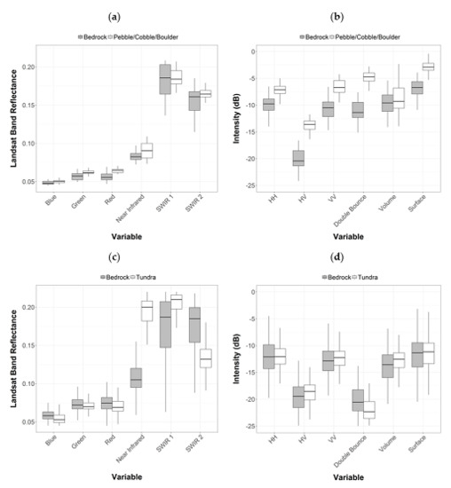
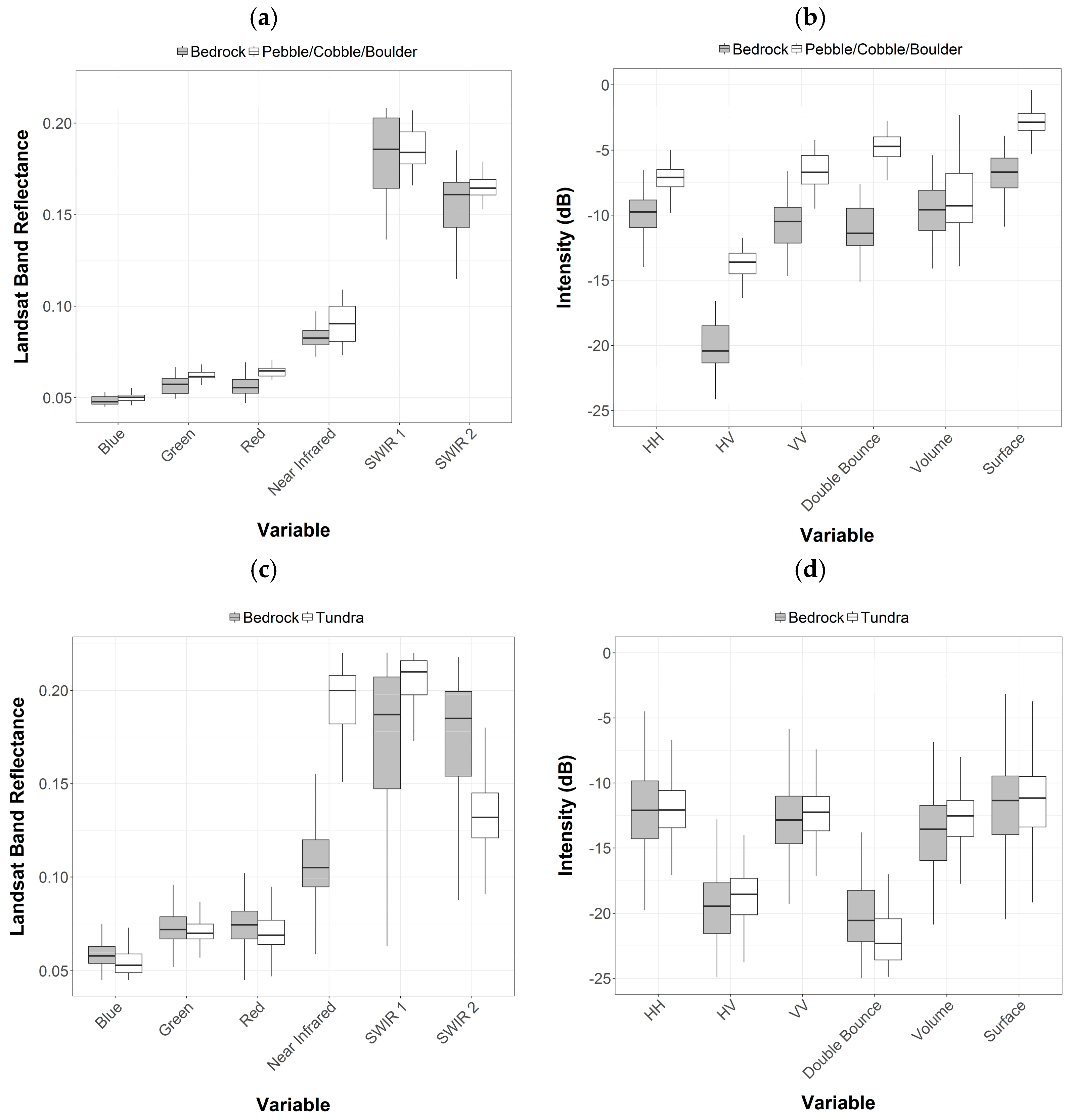
Further, because spectral signatures are affected by the chemical composition of the surface, confusion amongst substrate classes for models containing only Landsat 5 data is in part due to different substrates being composed of the same rock type (e.g., Pebble/Cobble/Boulder and Bedrock composed of the same sedimentary rocks). To demonstrate this, Figure 2 shows the spectral response of two features composed of the same material: one identified as Pebble/Cobble/Boulder, and the other as Bedrock. With the Landsat 5 image bands, many of the values for each class fall within a common range. However, with the quad pol RADARSAT-2 data, both exhibit distinct scattering behaviour (Figure 2). For the Pebble/Cobble/Boulder class, both the Freeman–Durden double bounce and HV intensity values are higher, and fall outside the range of values observed for the Bedrock sample. Similar observations were made for other features throughout the study area. The coarse resolution of the Landsat imagery also likely played a role in the increased confusion amongst several classes. Recently, very promising results for sediment type discrimination based on very high-resolution Pleiades data have been observed [71]. Given this, there is need for further research to better understand the effects of image resolution on the ability to differentiate substrate types.

By comparison, Random Forest models built with quad pol RADARSAT-2 and CDED data achieved better separability between many substrates, but also confused more vegetated and non-vegetated classes (e.g., Tundra versus Bedrock). Thus, independent overall accuracies were also lower (~13%) than models that included all predictor variables. This can similarly be explained by the fact that while vegetated and non-vegetated features typically absorb and reflect Near Infrared light differently, they can exhibit similar backscattering behavior. Figure 2 shows that with select SAR variables, values for Tundra and Bedrock fall mostly within a common range due to the short stature and low-density of vegetation being mostly transparent at C-band, resulting in both surfaces exhibiting relatively similar surface roughness. Conversely, because healthy vegetation strongly reflects Near Infrared light, values for Tundra are much higher and fall outside the range of values observed for Bedrock. Note that Sand/Mud were also misclassified more times by models containing quad pol RADARSAT-2 and CDED data, which is also due to both classes exhibiting similar surface roughness.

These results clearly demonstrate the complementarity of optical and SAR data for shoreline mapping (especially in cases where only coarse resolution optical imagery is used), as both were required to achieve acceptable accuracies for all land cover types. The quad pol RADARSAT-2 data was more effective in discriminating several of the substrate classes, while the Landsat 5 imagery was preferred for separating vegetated and non-vegetated classes. With the Landsat 5 and CDED data alone, it was only possible to accurately discriminate Water, Bedrock, Wetland, and Tundra (uer’s and prducer’s accuracies >/=80% achieved), while with the quad pol RADARSAT-2 and CDED data, only Water, Pebble/Cobble/Boulder, and Wetland were accurately classified (use’s and proucer’s accuracies >/=80%).

These findings are consistent with [16], who observed that both Landsat and RADARSAT-2 variables were among the most important inputs to their model. The authors of [17] also observed increased confusion between several substrate types when classifying SPOT-4 spectral bands and NDVI values using pixel-based Maximum Likelihood. With the addition of RADARSAT-2 HH, HV and VV values however, user’s and producer’s accuracies increased for several classes, including Sand (by 38% and 12%, respectively) and Wood/Substrate Mix (by 10% and 12%, respectively). The authors of [19] found that both quad pol RADARSAT-2 and SPOT-4 were useful in classifying multiple shoreline types using a hierarchical object-based classifier. With unsupervised SAR-based classifiers, the authors of [18] could differentiate features with different roughness, though observed confusion between classes with similar roughness (e.g., Tundra vs. Mixed Sediment). SAR data therefore contribute positively to differentiating substrates and are useful in classifying shoreline types, which contributes to the increasing portfolio of remote sensing coastal observation methods [72].

5.2. Comparing Performance of Random Forest Models Based on Quad Pol RADARSAT-2, Simulated Compact Polarized or Simulated Dual Polarized RCM Data in Combination with DEM Data

All models based on simulated RCM and CDED data achieved lower independent overall accuracies and were significantly different from the model based on quad pol RADARSAT-2 and CDED data (

Table 11. Evaluation metrics, including: independent overall accuracy (IOA), Kappa statistic values (K), and per-class user’s and producer’s accuracies (UA and PA) for Random Forest models generated with simulated RCM and CDED data. For comparison, results are included for the Random Forest model based on quad pol RADARSAT-2 and CDED data.

Model Run	Inputs for Models 3 to 10 Inputs Listed Are Additional to CDED Data	IOA (%)	K	Water		Sand/Mud		Mixed Sediment		Pebble/Cobble/Boulder		Bedrock		Wetland		Tundra
				UA (%)	PA (%)	UA (%)	PA (%)	UA (%)	PA (%)	UA (%)	PA (%)	UA (%)	PA (%)	UA (%)	PA (%)	UA (%)	PA (%)
3	Quad Pol RADARSAT-2; CDED	80	0.76	85	94	78	81	71	61	88	88	86	72	80	83	70	77
4	Simulated RCM High Resolution HH and HV	76	0.72	84	94	79	70	66	67	89	88	84	80	65	64	66	70
5	Simulated RCM Medium Resolution HH and HV	77	0.73	85	95	86	76	69	71	89	92	85	76	64	61	64	70
6	Simulated RCM High Resolution VV and VH	75	0.70	77	92	80	67	72	76	94	88	83	82	56	54	62	63
7	Simulated RCM Medium Resolution VV and VH	76	0.72	81	95	83	72	71	80	92	86	82	72	66	64	62	66
8	Simulated RCM High Resolution HH and VV	71	0.67	83	95	78	70	70	72	75	76	83	75	55	61	56	51
9	Simulated RCM Medium Resolution HH and VV	72	0.67	83	95	79	70	65	66	80	76	75	77	60	60	60	59
10	Simulated RCM High Resolution CP	76	0.72	83	95	80	72	67	64	88	84	79	76	68	77	69	65
11	Simulated RCM Medium Resolution CP	76	0.72	86	93	85	80	68	66	86	86	77	75	64	73	72	63

). Results from analyses used to address the first objective of this research explain, in part, why there is greater confusion between classes when Landsat 5 spectral data are excluded from the model. On the other hand, the decrease in accuracy observed as a result of the substitution of quad pol RADARSAT-2 for simulated RCM data is mostly related to the decrease in information content of the latter [24]. Conversely, the difference in NESZ values seems to have had less of an impact as indicated by the fact that user’s and producer’s accuracies did not decrease for classes with the lowest backscatter returns, including Water and Sand. This result is somewhat unexpected since at these incidence angles, values for these classes tend to fall close to or below both noise floors that were evaluated (i.e., below −19 dB for high, and below −25 dB for medium resolution data) [17]. Further research is necessary to understand and verify these observations.

For some classes, the substitution of RADARSAT-2 for simulated RCM data had a negligible or varied impact on user’s and producer’s accuracies (e.g., producer’s accuracies for Mixed Sediment were higher in all cases, though user’s accuracies were generally lower). Conversely, for the wetland class, this resulted in a large decrease in user’s and producer’s accuracies in all cases (>/=6%, and up to 29%). This is mostly as a result of increased confusion with Tundra, for which user’s and producer’s accuracies were also generally lower for models constructed with simulated RCM data. These results are consistent with [73] who similarly noted a decrease in the classification accuracy of wetlands when substituting quad pol RADARSAT-2 for simulated RCM data. Nevertheless, the authors found that the CP mode still achieved relatively high accuracies, and so suggested it was suitable for broad scale mapping. In [74], the authors found that outputs from the Freeman–Durden decomposition applied to quad pol data were more effective in identifying flooded vegetation compared to the m-Chi decomposition applied to simulated RCM CP data.

It is worth noting that the Wetland class may have been more accurately classified if steep incidence angle data were used. The authors of [17] observed that steep angle quad pol RADARSAT-2 was preferred for discriminating wetlands from tundra dominated by tall shrubs. This finding is sensible since, in theory, greater canopy penetration occurs at steeper angles resulting in greater sensitivity to sub-canopy conditions, including surface moisture and inundation [75]. However, since shallow angle imagery are also preferred for roughness information, fusion of multi-angle SAR data may be necessary to achieve high accuracies for all classes. Given the four-day repeat pass cycle of RCM, multi-angle datasets will likely be more easily attained, thus will be a focus of future work.

At similar polarizations, models constructed with high or medium resolution mode data were not significantly different overall (based on McNemar’s statistic; 95% confidence interval), indicating that these two modes can be used interchangeably in some cases. It is notable however, that with the VV and VH polarization, user’s and producer’s accuracies for Wetland were substantially higher (10%) for models constructed with medium resolution mode data. Though neither achieved acceptable accuracies for this class, this does indicate that one mode may still be more suitable for specific applications.

For the same imaging mode, models constructed with simulated CP, HH and HV, VV and VH data were also not significantly different overall, again indicating that these polarizations can be used interchangeably for certain applications. For both high and medium resolution mode datasets, models constructed with HH and VV polarization data achieved significantly lower independent overall accuracies. This result is consistent with others that have demonstrated the value of HV over HH and VV for shoreline mapping [16,17].

5.3. Comparing Performance of Random Forest Models Based on Quad Pol RADARSAT-2, Simulated Compact Polarized or Simulated Dual Polarized RCM Data in Combination with Landsat 5 and DEM Data

With the exception of models containing medium resolution CP data, all others constructed with simulated RCM, Landsat 5, and CDED variables were significantly different, with lower overall independent accuracies, than the first model based on all quad pol RADARSAT-2, Landsat 5, and CDED data (

Table 12. Evaluation metrics, including: independent overall accuracy (IOA), Kappa statistic values (K), and per-class user’s and producer’s accuracies (UA and PA) for Random Forest models generated with simulated RCM, Landsat 5, and CDED data. For comparison, results are included for the Random Forest model based on all Landsat 5, quad pol RADARSAT-2 and CDED variables.

Model Run	Inputs for Models 12 to 19 Inputs Listed Are Additional to the Landsat 5 and CDED Data	IOA (%)	K	Water		Sand/Mud		Mixed Sediment		Pebble/Cobble/Boulder		Bedrock		Wetland		Tundra
				UA (%)	PA (%)	UA (%)	PA (%)	UA (%)	PA (%)	UA (%)	PA (%)	UA (%)	PA (%)	UA (%)	PA (%)	UA (%)	PA (%)
1	Landsat 5; Quad Pol RADARSAT-2; CDED	93	0.91	96	99	94	94	86	92	94	88	95	95	89	89	94	92
12	Simulated RCM High Resolution HH and HV	89	0.87	96	98	88	89	83	87	94	89	96	95	81	81	87	86
13	Simulated RCM Medium Resolution HH and HV	90	0.89	96	98	91	93	85	90	95	90	98	94	81	81	87	86
14	Simulated RCM High Resolution VV and VH	89	0.87	96	98	87	89	82	84	94	88	95	95	81	82	87	86
15	Simulated RCM Medium Resolution VV and VH	90	0.89	96	98	93	92	86	92	94	89	95	95	81	82	88	86
16	Simulated RCM High Resolution HH and VV	87	0.85	96	98	88	89	79	80	85	83	94	94	81	81	87	86
17	Simulated RCM Medium Resolution HH and VV	88	0.86	96	98	90	89	83	84	89	86	92	94	80	82	86	84
18	Simulated RCM High Resolution CP	90	0.89	96	99	93	89	82	89	91	86	94	94	87	83	88	92
19	Simulated RCM Medium Resolution CP	91	0.90	96	98	93	93	87	90	91	88	94	94	86	86	90	89

). However, by comparison, differences between these models (i.e., Model 1 versus Models 12–19; Table 12) were less than differences between models constructed with quad pol RADARSAT-2 and CDED data, and simulated RCM and CDED data (i.e., Model 3 versus Models 4–11; Table 11). Thus, in this research, the type of SAR data (i.e., quad, dual or CP) had less of an impact on overall accuracy when the Landsat 5 optical data was also included as an input.

As was observed for models based on SAR and CDED data only, for some classes the substitution of quad pol for simulated RCM data had only a slight or varied impact on user’s and producer’s accuracies. For Water and Bedrock, for example, differences between models containing quad pol RADARSAT-2 and simulated RCM data ranged from 0% to 3%. For Wetland and Tundra, differences were higher in some cases, ranging from 2% to 9%, and from 0% to 8%, respectively (Table 12). Interestingly, all models constructed with simulated RCM, Landsat 5, and CDED data achieved accuracies that were considered to be within an acceptable range for operational mapping (i.e., >/=~80%, with the only exception being the user’s accuracy for Mixed Sediment which was 79% when classified with the Simulated RCM high resolution HH and VV imagery, Landsat 5, and CDED data). As such, it is expected that these data, which will be available at a greater temporal frequency and wider swath width than RADARSAT-2, will complement current efforts focused at mapping shorelines throughout the Canadian Arctic [16,17,18].

Note that these results are consistent with [76] who used Random Forests to classify Peatlands in Southern Ontario. The authors similarly observed that when classified in combination with Landsat 8 optical and Shuttle RADAR Topography Mission DEM data, there was not a significant difference between models that contained quad pol RADARSAT-2 or simulated RCM data.

With the exception of the VH and VV polarization, models constructed with high or medium resolution mode data were not significantly different at similar polarizations, again demonstrating that in some cases both imaging modes can be used interchangeably. In fact, the maximum difference in user’s and producer’s accuracies between models containing high and medium resolution data was 5%, and independent overall accuracies only differed by 1%. For VH and VV polarization however, a statistically significant difference was observed between models constructed with high and medium resolution mode data, with the latter achieving higher accuracies for Sand/Mud and Mixed Sediment.

Similarly, with similar imaging modes, models constructed with simulated CP, HH and HV, and VV and VH data were not significantly different overall. Notably though, user’s and producer’s accuracies for Wetland were highest with CP data. Since these features typically represent important species habitat and are sensitive to the effects of climate change and of oiling, it is essential that they are accurately classified. This justifies preference for this beam mode for certain applications, including shoreline mapping. As was observed when Landsat 5 data were excluded from models (Table 11), those constructed with simulated HH and VV data achieved significantly lower overall accuracies compared to models containing other data for other polarizations, which is again consistent with observations by others that HV is generally preferred over HH and VV for shoreline mapping [16,17].

5.4. Determining the Extent to which Model Data Load Can Be Reduced without Impacting or Possibly Improving Overall Accuracy

Given the number of datasets evaluated in this research, the decision was made to select one to evaluate the effect of reducing the model data load. Given that [16] already evaluated the effect of reducing the dimensionality of the quad pol RADARSAT-2, Landsat 5, and CDED dataset, we chose to evaluate the Simulated RCM medium resolution mode CP, Landsat 5, and CDED dataset (i.e., Model 19). This dataset was also evaluated because it achieved the highest accuracy of all models containing simulated RCM data, performing most similarly to the model containing quad pol RADARSAT-2, Landsat 5, and CDED data.

Results from this analysis indicate that multiple methods can be effective in reducing the number of inputs to Random Forests models, without affecting overall accuracy (

Table 13. Evaluation metrics, including: independent overall accuracy (IOA), Kappa statistic values (K), and per-class user’s and producer’s accuracies (UA and PA) for Random Forest models generated with RCM medium resolution mode CP, Landsat 5, and CDED dataset (i.e., Model 19) based on different sets of variables. Variables included in all three models constructed as part of the variable reduction process are bolded and italicized.

Inputs (Listed in Order of Importance)	IOA (%)	K	Water		Sand/Mud		Mixed Sediment		Pebble/Cobble/ Boulder		Bedrock		Wetland		Tundra
			UA (%)	PA (%)	UA (%)	PA (%)	UA (%)	PA (%)	UA (%)	PA (%)	UA (%)	PA (%)	UA (%)	PA (%)	UA (%)	PA (%)
All Variables	91	0.90	96	98	93	93	87	90	91	88	94	94	86	86	90	89
Top 10 of all non-correlated variables m-Chi Decomposition: volume scattering, NDMI, Near Infrared/SWIR-1, Red/SWIR-2, Tasseled Cap Transformation: Greenness, Shannon Entropy Polarimetry, Relative Phase, SWIR-1/SWIR-2, S1, Julian day of the RADARSAT-2 Acquisition	89	0.88	93	96	92	87	84	94	91	87	94	90	86	82	86	89
10 variables with the highest importance from all variables: m-Chi Decomposition: volume scattering; RR intensity; NDMI; RV intensity; Near Infrared/SWIR-1; Red/SWIR-2; RH intensity; DEM; Shannon Entropy Intensity; Tasseled Cap Transformation: Wetness	89	0.87	94	94	91	88	80	89	91	86	91	90	85	87	91	89
10 remaining variables following backward selection process m-Chi Decomposition: volume scattering; RR Intensity; RV Intensity; NDMI; Red/SWIR-2; Tasseled Cap Transformation: Greenness; Near Infrared/SWIR-1; Green/SWIR-2; NDWI; Blue/Near Infrared	90	0.89	98	98	93	93	85	90	90	86	93	92	86	84	87	89

). In this research, performance of the model did not vary significantly based on the reduction method, thus demonstrating, as others have observed [16], that Random Forests is not highly sensitive to the type and number of inputs. We expect that this is especially the case here given that many variables were highly correlated, and classes were highly separable.

It is worth noting that, for the first method, a threshold value of r > 0.5 was found to be effective in reducing redundant information without affecting classifier accuracy. In addition, the second method, while not taking into account the possible spreading of importance values among correlated inputs [64], still achieved the same accuracy, while also being the most efficient approach (in terms of computation expense and required user intervention). These results also show that the CDED data was not needed for accurate discrimination of the land covers evaluated in this research (Table 13). We suspect that this is due to a combination of the DEM being provided at a coarse resolution, and the fact that most features in the study area are relatively low lying and flat.

5.5. Limitations

Although effort has been made to simulate and evaluate data that closely represents that which will be available from RCM, further research is necessary to validate these results once real RCM data becomes available. In this research, simulations were based on projected (and also nominal) NESZ values, which may differ with real RCM data (in addition to also differing by beam mode). The effect of image resolution on classifier accuracy also requires further study since the high-resolution mode data were generated at the same pixel spacing as the original quad pol RADARSAT-2 data, and the medium resolution mode data were only resampled from 8.2 to 16 m. In particular, it is notable that the impact of resolution on variance may not have been adequately represented. Nonetheless, the potential for similar classification accuracies with data that can be acquired across much larger swaths has been demonstrated, and should be considered an attractive option to users, especially for operational mapping and monitoring programs.

6. Conclusions and Future Work

The major conclusions of this research are:

(1)

Optical and SAR data provide relevant and complementary information for mapping shoreline types. Given the imagery and variables tested in this research, SAR data were required for accurate discrimination of substrate types, while optical data were required for accurate discrimination of some vegetated and non-vegetated classes.

(2)

Simulated RCM and CDED data achieved significantly lower overall accuracies than quad pol RADARSAT-2 and CDED data, with the wetland class being most affected by the difference in information content of the SAR data.

(3)

When classified in combination with Landsat 5 variables, model accuracy was less affected by the SAR data type. All simulated RCM beam modes and polarizations evaluated achieved high accuracies when classified together with Landsat 5 and CDED data. However, the best results were achieved with the medium resolution CP data.

(4)

Whether classified with CDED data, or a combination of CDED and Landsat 5 data, models based on simulated CP, HH and HV, or VH and VV imagery achieved results that were not significantly different overall. This indicates that these polarizations could be used interchangeably in some cases to achieve approximately the same classification accuracies.

(5)

Whether classified with CDED data, or a combination of CDED and Landsat 5 data, models based on simulated high or medium resolution mode imagery were not significantly different at similar polarizations, indicating that these beam modes could be used interchangeably, in some cases, to achieve approximately the same classification accuracies.

(6)

Multiple different variable reduction processes can be used to greatly reduce the number of inputs provided to the model without affecting classifier accuracy. All variable reduction methods tested in this research yielded models that were not significantly different.

Based on these results, and given the recent release of freely available Earth Observation data at higher spatial resolutions, including Sentinel 2A [77], and the Arctic DEM [78], future work will focus on evaluating these data for a higher resolution shoreline type map, and for continued monitoring of change and improving emergency preparedness in the Arctic. Given the recent and very promising results for sediment type discrimination based on very high-resolution Pleiades imagery [71], efforts will also focus on evaluating the effects of image resolution on the ability to differentiate sediments using optical data alone. Additionally, we plan to evaluate both multi-temporal and multi-angle RADARSAT-2 and RCM data, once it becomes available.

References

1. Rampton, V. Surficial Geology of the Mackenzie Delta. In Geological Survey of Canada (GSC), Marine Science Atlas of the Beaufort Sea: Geology and Geophysics; Minister of Supply and Services Canada: Ottawa, ON, Canada, 1987. [Google Scholar]
2. Rampton, V. Surficial Geology of the Tuktoyaktuk Peninsula. In Geological Survey of Canada (GSC), Marine Science Atlas of the Beaufort Sea: Geology and Geophysics; Minister of Supply and Services Canada: Ottawa, ON, Canada, 1987. [Google Scholar]
3. Harper, J.; Owens, E.; Wiseman, W. Arctic Beach Processes and the Thaw of Ice-Bonded Sediments in the Littoral Zone. In Proceedings of the 3rd International Permafrost Conference, Edmonton, AB, Canada, 10–13 July 1978. [Google Scholar]
4. Kobayashi, N.; Atkan, D. Thermoerosion of Frozen Sediment under Wave Action. J. Waterw. Port. Coast. Ocean Div. 1986, 112, 140–158. [Google Scholar] [CrossRef]
5. Dallimore, S.; Wolfe, S.; Solomon, S. Influence of Ground Ice and Permafrost on Coastal Evolution, Richards Island, Beaufort Sea Coast, N.W.T. Can. J. Earth Sci. 1996, 33, 664–675. [Google Scholar] [CrossRef]
6. Sturm, M.; Racine, C.; Tape, K. Climate change: Increasing shrub abundance in the Arctic. Nature 2001, 411, 546. [Google Scholar] [CrossRef] [PubMed]
7. Tape, K.; Sturm, M.; Racine, C. The evidence for shrub expansion in northern Alaska and the Pan-Arctic. Glob. Chang. Biol. 2006, 12, 686–702. [Google Scholar] [CrossRef]
8. Sokolov, V.; Ehrich, D.; Yoccoz, N.G.; Sokolov, A.; Lecomte, N. Bird communities of the Arctic shrub tundra of Yamal: Habitat specialists and generalists. PLoS ONE 2012, 7, e50335. [Google Scholar] [CrossRef] [PubMed] [Green Version]
9. Reynolds, J.; Tenhunen, J. Ecosystem response, resistance, resilience, and recovery in Arctic landscapes: Introduction. In Landscape Function and Disturbance in Arctic Tundra; Ecological Studies, Reynolds, J., Tenhunen, J., Eds.; Springer: Berlin, Germany, 1996; pp. 3–18. ISBN 978-3-662-01145-4. [Google Scholar]
10. Intergovernmental Panel on Climate Change. Climate Change 2014: Synthesis Report. Contribution of Working Groups I, II and III to the Fifth Assessment Report of the Intergovernmental Panel on Climate Change; Core Writing Team, Pachauri, R.K., Meyer, L.A., Eds.; IPCC: Geneva, Switzerland, 2014; p. 151. [Google Scholar]
11. Ellis, B.; Brigham, L. Arctic Marine Shipping Assessment 2009 Report; Arctic Council: Tromsø, Norway, 2009. [Google Scholar]
12. Wilson, K.; Falkingham, J.; Melling, H.; De Abreu, R. Shipping in the Canadian Arctic: Other possible climate change scenarios. In Proceedings of the International Geoscience and Remote Sensing Symposium, Anchorage, AK, USA, 20–24 September 2004. [Google Scholar]
13. Owens, E.; Sergy, G. The Arctic SCAT Manual: A Field Guide to the Documentation of Oiled Shorelines in Arctic Environments; Environment Canada: Edmonton, AB, Canada, 2004.
14. Owens, E. Primary Shoreline Types of the Canadian North; Environment Canada: Ottawa, ON, Canada, 2010.
15. Owens, E.; Sergy, G. The SCAT Manual—A Field Guide to the Documentation and Description of Oiled Shorelines; Environment Canada: Edmonton, AB, Canada, 2000.
16. Banks, S.; Millard, K.; Pasher, J.; Richardson, M.; Wang, H.; Duffe, J. Assessing the Potential to Operationalize Shoreline Sensitivity Mapping: Classifying Multiple Wide Fine Quad Polarized RADARSAT-2 and Landsat 5 Scenes with a Single Random Forest Model. Remote Sens. 2015, 40, 13528–13563. [Google Scholar] [CrossRef]
17. Banks, S.; King, D.; Merzouki, A.; Duffe, J. Assessing RADARSAT-2 for Mapping Shoreline Cleanup and Assessment Technique (SCAT) Classes in the Canadian Arctic. Can. J. Remote Sens. 2014, 40, 243–267. [Google Scholar] [CrossRef]
18. Banks, S.; King, D.; Merzouki, A.; Duffe, J. Characterizing Scattering Behaviour and Assessing Potential for Classification of Arctic Shore and Near-Shore Land Covers with Fine Quad-Pol RADARSAT-2 Data. Can. J. Remote Sens. 2014, 40, 291–314. [Google Scholar] [CrossRef]
19. Demers, A.; Banks, S.; Pasher, J.; Duffe, J.; LaForest, S. A comparative analysis of object-based and pixel-based classification of RADARSAT-2 C-band and optical satellite data for mapping shoreline types in the Canadian arctic. Can. J. Remote Sens. 2015, 41, 1–19. [Google Scholar] [CrossRef]
20. Flett, D.; Crevier, Y.; Girard, R. The RADARSAT Constellation Mission: Meeting the Government of Canada’s Needs and Requirements. In Proceedings of the International Geoscience and Remote Sensing Symposium, Cape Town, South Africa, 12–17 July 2009. [Google Scholar]
21. Séguin, G.; Gratton, D. RADARSAT Constellation Mission Overview. In Proceedings of the ASTRO 2010 15th CASI Canadian Aeronautics and Space Institute Conference, Toronto, ON, Canada, 4–6 May 2010. [Google Scholar]
22. Thompson, A. Overview of the RADARSAT Constellation Mission. Can. J. Remote Sens. 2015, 41, 401–407. [Google Scholar] [CrossRef]
23. RADARSAT-2 Product Description. Available online: http://mdacorporation.com/docs/default-source/technical-documents/geospatial-services/52–1238_rs2_product_description.pdf?sfvrsn=10 (accessed on 27 September 2017).
24. Raney, R. Hybrid-Polarity SAR Architecture. IEEE Geosci. Remote Sens. 2007, 45, 3397–3404. [Google Scholar] [CrossRef]
25. Charbonneau, F.; Brisco, B.; Raney, K.; McNairn, H.; Chen, L.; Vachon, P.; Shang, J.; Champagne, C.; Merzouki, A.; Geldsetzer, T.; et al. Compact Polarimetry Overview and Applications Assessment. Can. J. Remote Sens. 2010, 36, S298–S315. [Google Scholar] [CrossRef]
26. Breiman, L. Random forests. Mach. Learn. 2001, 45, 5–32. [Google Scholar] [CrossRef]
27. Millard, K.; Richardson, M. Wetland mapping with LiDAR derivatives, SAR polarimetric decompositions, and LiDAR-SAR fusion using a random forest classifier. Can. J. Remote Sens. 2013, 39, 290–307. [Google Scholar] [CrossRef]
28. Millard, K.; Richardson, M. On the importance of training data sample selection in random forest image classification: A case study in peatland ecosystem mapping. Remote Sens. 2015, 7, 8489–8515. [Google Scholar] [CrossRef]
29. Liaw, A.; Wiener, M. Classification and regression by Random Forest. R News 2002, 2, 18–22. [Google Scholar]
30. Lawrence, R.; Wood, S.; Sheley, R. Mapping invasive plant species using hyperspectral imagery and Breiman Cutler classifications (randomForest). Remote Sens. Environ. 2006, 100, 356–362. [Google Scholar] [CrossRef]
31. Waske, B.; Braun, M. Classifier ensembles for land cover mapping using multi-temporal SAR imagery. ISPRS J. Photogramm. Remote Sens. 2009, 64, 450–457. [Google Scholar] [CrossRef]
32. Rodriguez-Galiano, V.; Chica-Olmo, M.; Abarca-Hernandez, F.; Atkinson, P.; Jeganathan, C. Random Forest classification of Mediterranean land cover using multi-seasonal imagery and multi-seasonal texture. Remote Sens. Environ. 2012, 121, 93–107. [Google Scholar] [CrossRef]
33. Attarchi, S.; Gloaguen, R. Classifying complex mountainous forests with L-Band SAR and Landsat data integration: A comparison among different machine learning methods in the Hyrcanian Forest. Remote Sens. 2014, 6, 3624–3647. [Google Scholar] [CrossRef]
34. Deschamps, B.; McNairn, H.; Shang, J.; Jiao, X. Towards operational radar-only crop type classification: Comparison of a traditional decision tree with a random forest classifier. Can. J. Remote Sens. 2012, 38, 60–68. [Google Scholar] [CrossRef]
35. Ghimire, B.; Rogan, J.; Miller, J. Contextual land-cover classification: Incorporating spatial dependence in land-cover classification models using random forests and the Ghetis statistic. Remote Sens. Lett. 2010, 1, 45–54. [Google Scholar] [CrossRef]
36. Gislason, P.; Benediktsson, J.; Sveinsson, J. Random forests for land cover classification. Pattern Recognit. Lett. 2006, 27, 294–300. [Google Scholar] [CrossRef]
37. Sonobe, R.; Tani, H.; Wang, X.; Kobayashi, N.; Shimamura, H. Random forest classification of crop type using multi-temporal TerraSAR-X dual-polarimetric data. Remote Sens. Lett. 2014, 5, 157–164. [Google Scholar] [CrossRef]
38. Pal, M. Random forest classifier for remote sensing classification. Int. J. Remote Sens. 2005, 26, 217–222. [Google Scholar] [CrossRef]
39. Adam, E.; Mutanga, O.; Odindi, J.; Abdel-Rahman, E.M. Land-use/cover classification in a heterogeneous coastal landscape using RapidEye imagery: Evaluating the performance of random forest and support vector machines. Int. J. Remote Sens. 2014, 35, 3440–3458. [Google Scholar] [CrossRef]
40. Akar, Ö.; Güngör, O. Classification of multispectral images using Random Forest algorithm. J. Geod. Geoinf. 2012, 1, 105–112. [Google Scholar] [CrossRef]
41. Corcoran, J.; Knight, J.; Gallant, A. Influence of multi-source and multi-temporal remotely sensed and ancillary data on the accuracy of random forest classification in northern Minnesota. Remote Sens. 2013, 5, 3212–3238. [Google Scholar] [CrossRef]
42. Gillie, R. Aerial Video Shoreline Survey Coronation Gulf and Queen Maud Gulf, Northwest Territories, August 18–25; AXYS Environmental Consulting Ltd.: Sidney, BC, Canada, 1995. [Google Scholar]
43. Wynja, V.; Demers, A.; LaForest, S.; Lacelle, M.; Pasher, J.; Duffe, J.; Chaudhary, B.; Wang, H.; Giles, T. Mapping coastal information across Canada’s northern regions based on low-altitude helicopter videography in support of environmental emergency preparedness efforts. J. Coast. Res. 2014, 31, 276–290. [Google Scholar] [CrossRef]
44. United States Geological Service, Landsat Surface Reflectance High Level Data Products. Available online: http://landsat.usgs.gov/CDR_LSR.php (accessed on 30 September 2014).
45. Woodhouse, I.H. Introduction to Microwave Remote Sensing; CRC Press: Boca Raton, FL, USA, 2006. [Google Scholar]
46. Freeman, A.; Durden, S.L. A three component scattering model for polarimetric SAR data. IEEE Trans. Geosci. Remote Sens. 1998, 36, 963–973. [Google Scholar] [CrossRef]
47. Cloude, S.; Pottier, E. An entropy based classification scheme for land applications of polarimetric SAR. IEEE Trans. Geosci. Remote Sens. 1997, 35, 68–78. [Google Scholar] [CrossRef]
48. Touzi, R. Target scattering decomposition in terms of roll-invariant target parameters. IEEE Geosci. Remote Sens. 2007, 45, 73–84. [Google Scholar] [CrossRef]
49. Touzi, R.; Goze, S.; Le Toan, T.; Lopes, A.; Mougin, E. Polarimetric discriminators for SAR images. IEEE Geosci. Remote Sens. 1992, 30, 973–980. [Google Scholar] [CrossRef]
50. Raney, R.; Cahill, J.; Patterson, G.; Bussey, D. The m-chi decomposition of hybrid dual-polarimetric radar data with application to lunar craters. J. Geophys. Res. 2012, 117, 1–8. [Google Scholar] [CrossRef]
51. Lee, J.; Pottier, E. Polarimetric Radar Imaging: From Basics to Applications; CRC Press, Taylor & Francis: Boca Raton, FL, USA, 2009; p. 397. [Google Scholar]
52. Cloude, S.; Goodenough, D.; Chen, H. Compact decomposition theory. IEEE Trans. Geosci. Remote Sens. 2012, 9, 28–32. [Google Scholar] [CrossRef]
53. Truong-Loi, M.; Freeman, A.; Dubois-Fernandez, P.; Pottier, E. Estimation of soil moisture and Faraday rotation from bare surfaces using compact polarimetry. IEEE Trans. Geosci. Remote Sens. 2009, 47, 3608–3615. [Google Scholar] [CrossRef]
54. Tucker, C.; Sellers, P. Satellite remote sensing of primary productivity. Int. J. Remote Sens. 1986, 7, 1395–1416. [Google Scholar] [CrossRef]
55. Gao, B. NDWI—A normalized difference water index for remote sensing of vegetation liquid water from space. Remote Sens. Environ. 1996, 58, 257–266. [Google Scholar] [CrossRef]
56. Huete, A. A Soil-Adjusted Vegetation Index (SAVI). Remote Sens. Environ. 1988, 25, 295–309. [Google Scholar] [CrossRef]
57. Wang, L.; Qu, J. NMDI: A normalized multi-band drought index for monitoring soil and vegetation moisture with satellite remote sensing. Geophys. Res. Lett. 2007, 34, L20405. [Google Scholar] [CrossRef]
58. Crist, E.; Richard, C. A physically-based transformation of Thematic Mapper data—The TM Tasseled Cap. IEEE Geosci. Remote Sens. Lett. 1984, 3, 256–263. [Google Scholar] [CrossRef]
59. Red Hen Systems: VMS-333 and VMS-Mobile User Guide. Available online: https://www.redhensystems.com/sites/default/files/vms333_userguide_v1.228-15-2016.pdf (accessed on 15 January 2017).
60. R Core Team. R: A Language and Environment for Statistical Computing; R Foundation for Statistical Computing: Vienna, Austria, 2007; Available online: https://www.R-project.org/ (accessed on 15 January 2017).
61. Hijmans, R.J. Raster: Geographic Data Analysis and Modeling. R Package Version 2.5-8. Available online: https://CRAN.R-project.org/package=raster (accessed on 15 January 2017).
62. Pebesma, E.J.; Bivand, R.S. Classes and methods for spatial data in R. R News 2005, 5, 9–13. [Google Scholar]
63. Bivand, R.S.; Pebesma, E.; Gomez-Rubio, V. Applied Spatial Data Analysis with R, 2nd ed.; Springer: New York, NY, USA, 2013; Available online: http://www.asdar-book.org/ (accessed on 15 January 2017).
64. Genuer, R.; Poggi, J.; Tuleau-Malot, C. Variable selection using random forests. Pattern Recognit. Lett. 2010, 31, 2225–2236. [Google Scholar] [CrossRef]
65. Behnamian, A.; Millard, K.; Banks, S.; White, L.; Richardson, M.; Pasher, J. A Systematic Approach for Variable Selection with Random Forests: Achieving Stable Variable Importance Values. IEEE Trans. Geosci. Remote Sens. 2017, 99. [Google Scholar] [CrossRef]
66. Foody, G. Thematic map comparison: Evaluating the statistical significance of differences in classification accuracy. Photogramm. Eng. Remote Sens. 2004, 70, 627–633. [Google Scholar] [CrossRef]
67. Bradley, J. Distribution-Free Statistical Tests; Prentice-Hall: Englewood Cliffs, NJ, USA, 1968; p. 388. [Google Scholar]
68. Agresti, A. An Introduction to Categorical Data Analysis; Wiley: New York, NY, USA, 1996; p. 312. [Google Scholar]
69. Henderson, F.; Lewis, A. Manual of Remote Sensing: Principles and Applications of Imaging Radar, 2nd ed.; Wiley: New York, NY, USA, 1996. [Google Scholar]
70. Peake, W.; Oliver, T. The Response of Terrestrial Surface at Microwave Frequencies; Ohio State University Columbus Electroscience Lab, Defense Technical Information Center: Columbus, OH, USA, 1971. [Google Scholar]
71. Chen, Z; Pasher, J.; Duffe, J.; Behnamian, A. Mapping Arctic Coastal Ecosystems with High Resolution Optical Satellite Imagery Using a Hybrid Classification Approach. Can. J. Remote Sens. 2017, 1–15. [Google Scholar] [CrossRef]
72. Liu, Y.; Kerkering, H.; Weisberg, R.H. Coastal Ocean Observing Systems; Elsevier (Academic Press): London, UK, 2015. [Google Scholar]
73. Brisco, B.; Li, K.; Tedford, B.; Charbonneau, F.; Yun, S.; Murnaghan, K. Compact Polarimetry assessment for ride and wetland mapping. Int. J. Remote Sens. 2013, 34, 1949–1964. [Google Scholar] [CrossRef]
74. White, L.; Brisco, B.; Dabboor, M.; Schmitt, A.; Pratt, A. A collection of SAR methodologies for monitoring wetlands. Remote Sens. 2015, 7, 7615–7645. [Google Scholar] [CrossRef] [Green Version]
75. Ramsey, E. Radar Remote Sensing of Wetlands. In Remote Sensing Change Detection: Environmental Monitoring Methods and Applications; Lunetta, R., Elvidge, C., Eds.; Ann Arbor Press: Chelsea, MA, USA, 1998; pp. 211–243. [Google Scholar]
76. White, L.; Millard, K.; Banks, S.; Richardson, M.; Pasher, J.; Duffe, J. Moving to the RADARSAT Constellation Mission: Comparing Synthesized Compact Polarimetry and Dual Polarimetry Data with Fully Polarimetric RADARSAT-2 Data for Image Classification of Peatlands. Remote Sens. 2017, 9, 573. [Google Scholar] [CrossRef]
77. Copernicus: Observing the Earth. Available online: http://www.esa.int/Our_Activities/Observing_the_Earth/Copernicus/Overview4 (accessed on 27 September 2017).
78. Polar Geospatial Centre: Arctic DEM. Available online: https://www.pgc.umn.edu/data/arcticdem/ (accessed on 27 September 2017).
Figure 1. Map showing the footprint of RADARARSAT-2 and Landsat 5 scenes used in this research, and the five sites where helicopter videography data and geotagged photos were collected. Values on each line segment indicate the approximate length of shoreline covered by each videography survey (described subsequently). This figure is adapted from [16].
Remotesensing 09 01206 g001
Figure 2. Box-and-Whisker plots (top = 25th percentile, middle = 50th percentile, bottom = 75th percentile, whiskers = 5th and 95th percentile) to show sample values for two shorelines composed of the same rock type but representing different shoreline classes (Bedrock and Pebble Cobble Boulder): (a) Landsat 5 band reflectance values; (b) quad pol RADARSAT-2 intensity, and Freeman–Durden decomposition values; and (c,d) for all training and validation sites for the Bedrock and Tundra class, Landsat 5 band reflectance values and quad pol RADARSAT-2 intensity, and Freeman–Durden decomposition values, respectively. Note that the range of values for Bedrock differ (i.e., among (ad)), which is due to the samples from (a,b) being from one location and rock type, while those for (c,d) were for all rock types sampled throughout the entire study area.
Remotesensing 09 01206 g002