Semi-Automated Surface Water Detection with Synthetic Aperture Radar Data: A Wetland Case Study


 ,
,
Abstract
:
1. Introduction
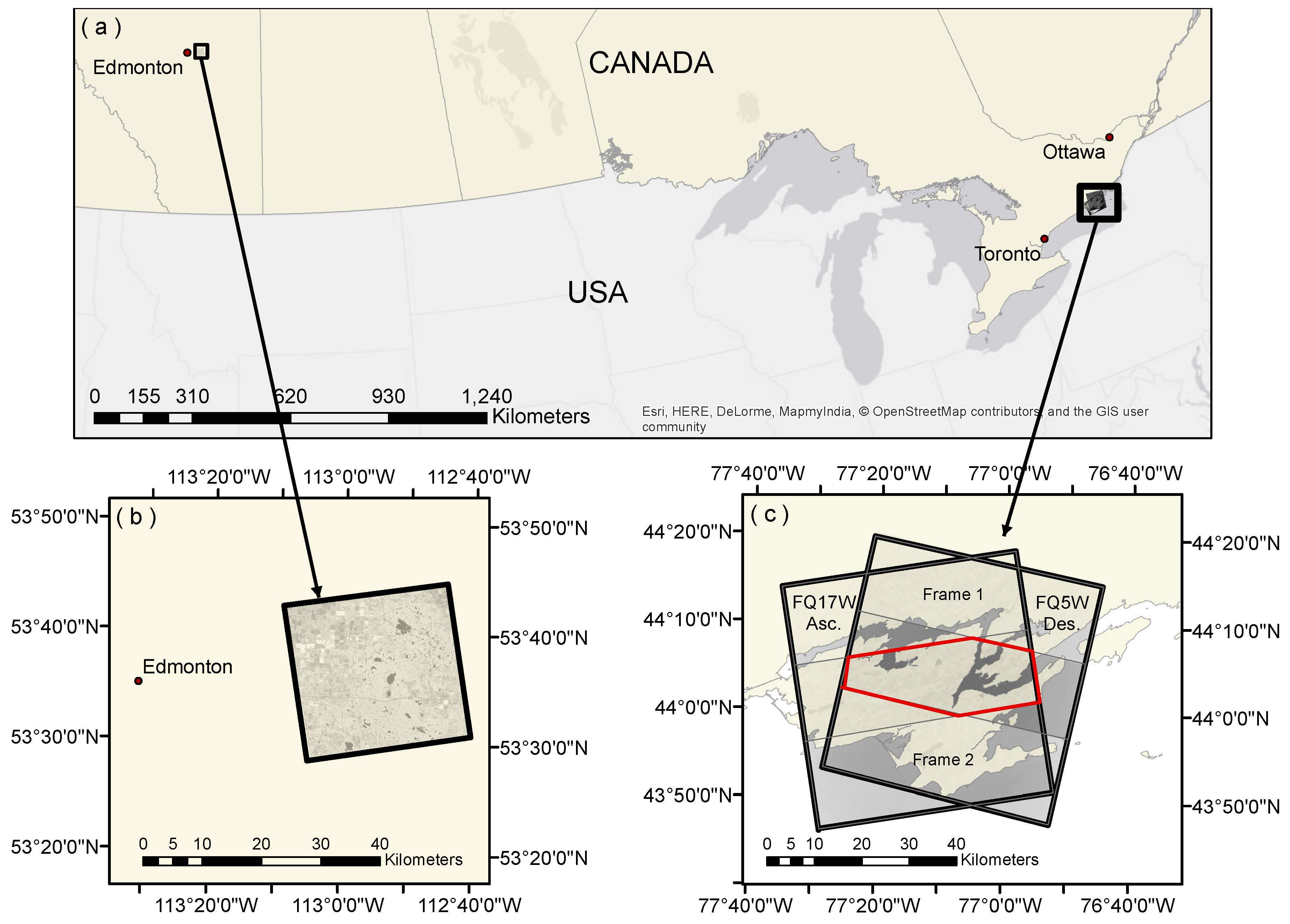
2. Study Areas and Data Acquisition
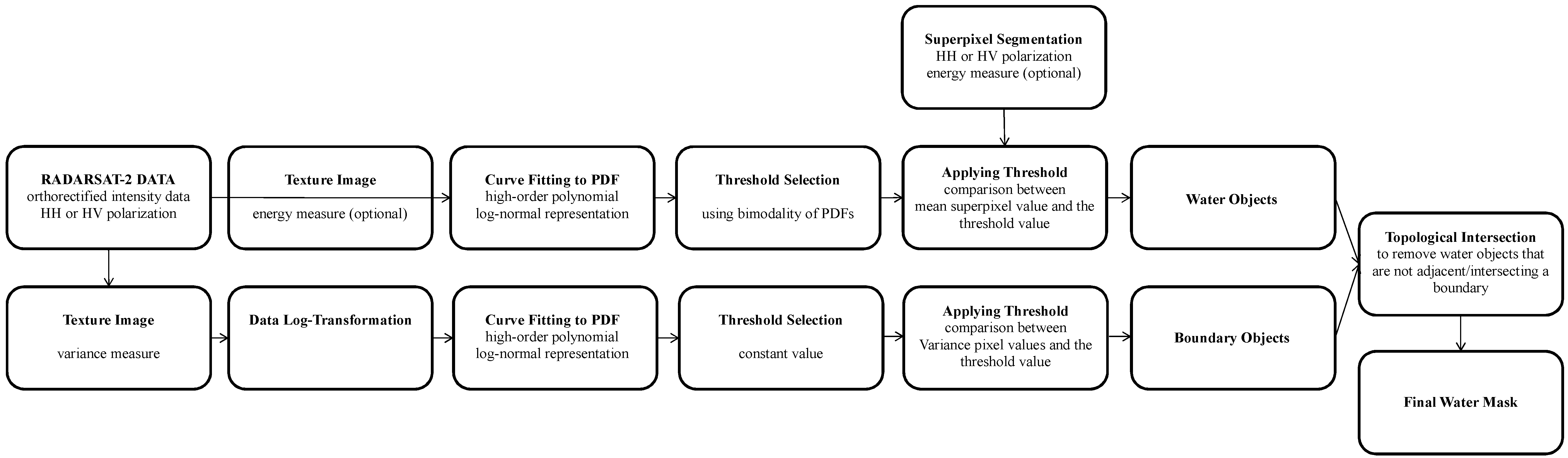
3. Methodology
3.1. Image Processing
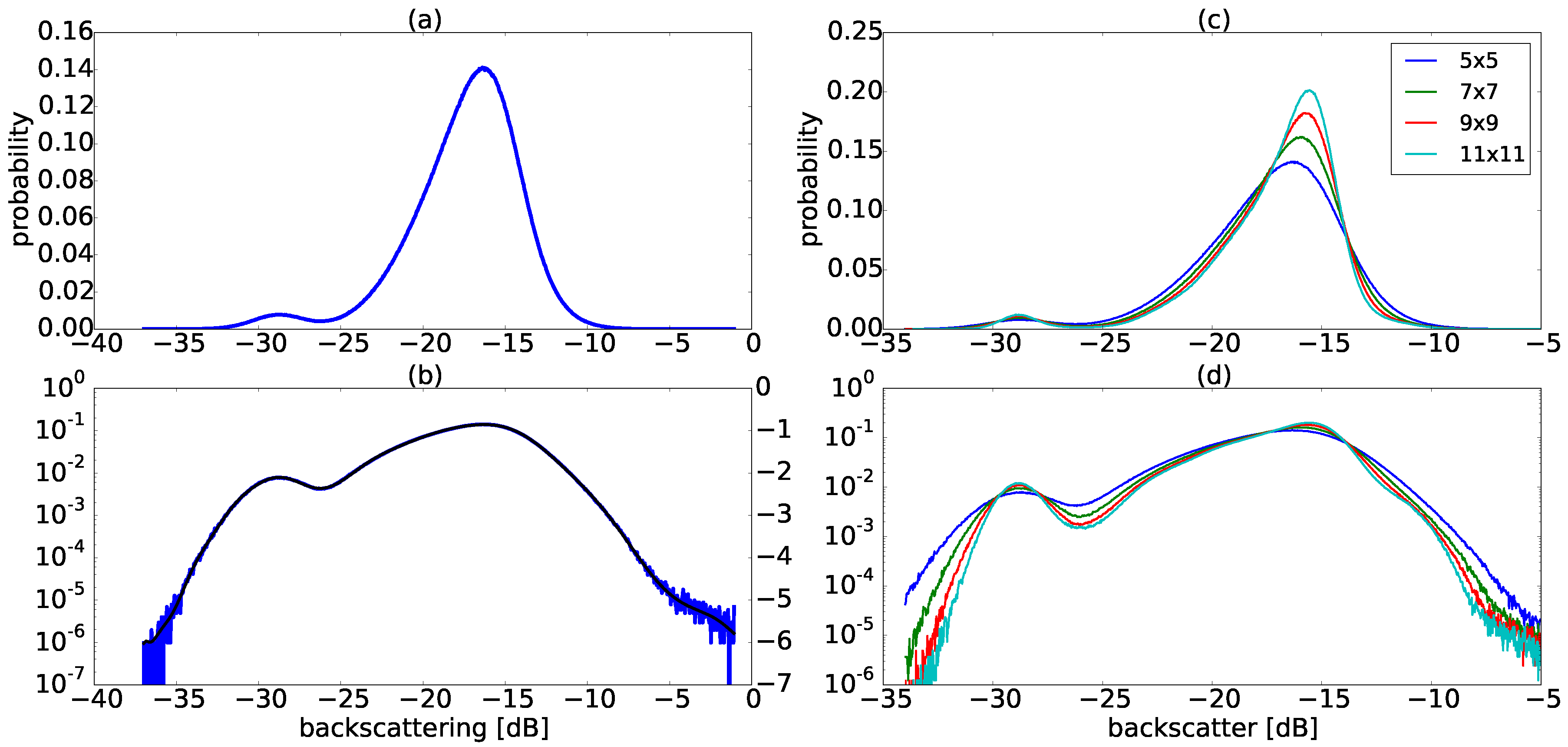
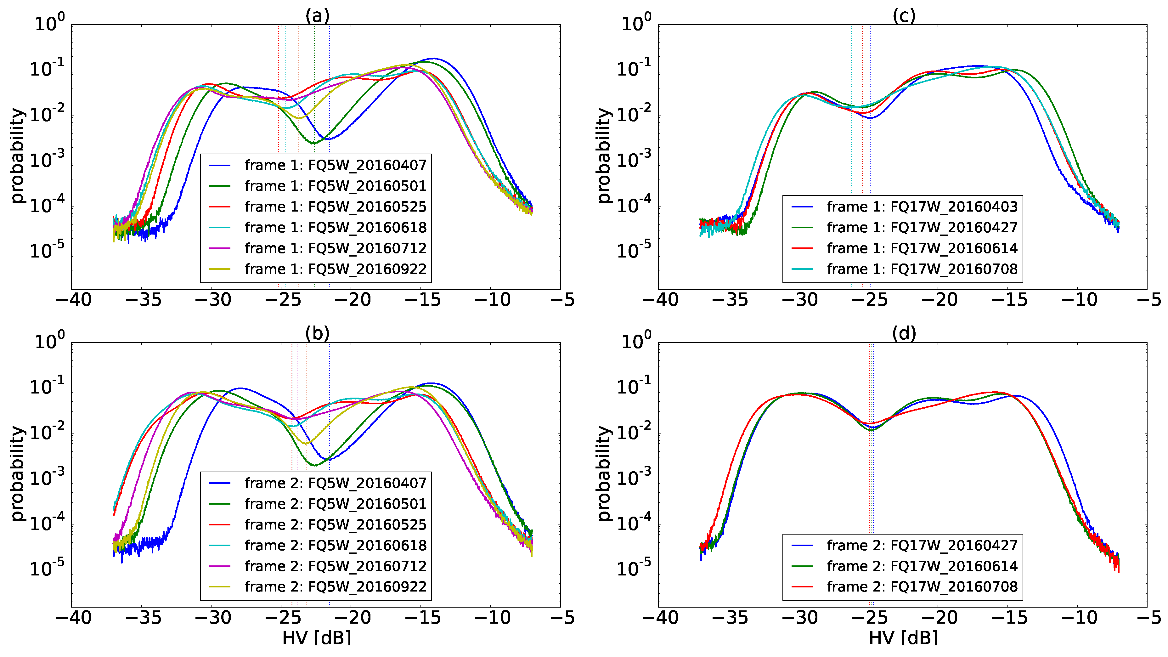
3.2. Threshold Selection
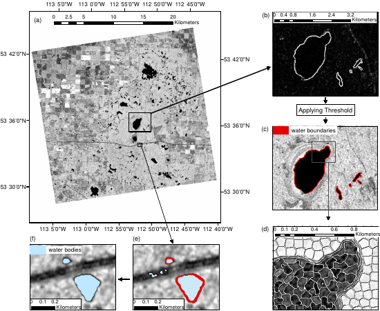
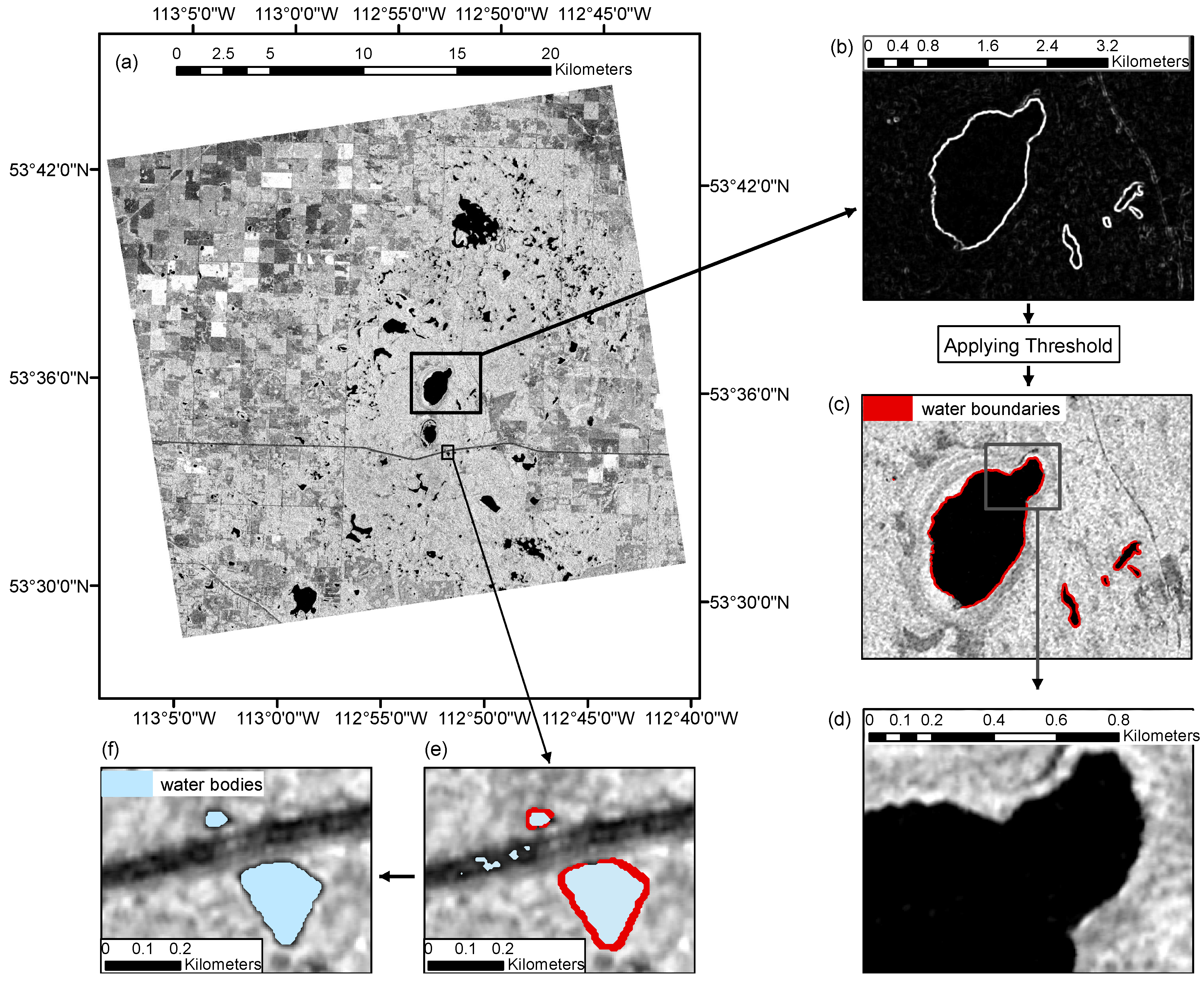
3.2.1. Surface Water Detection
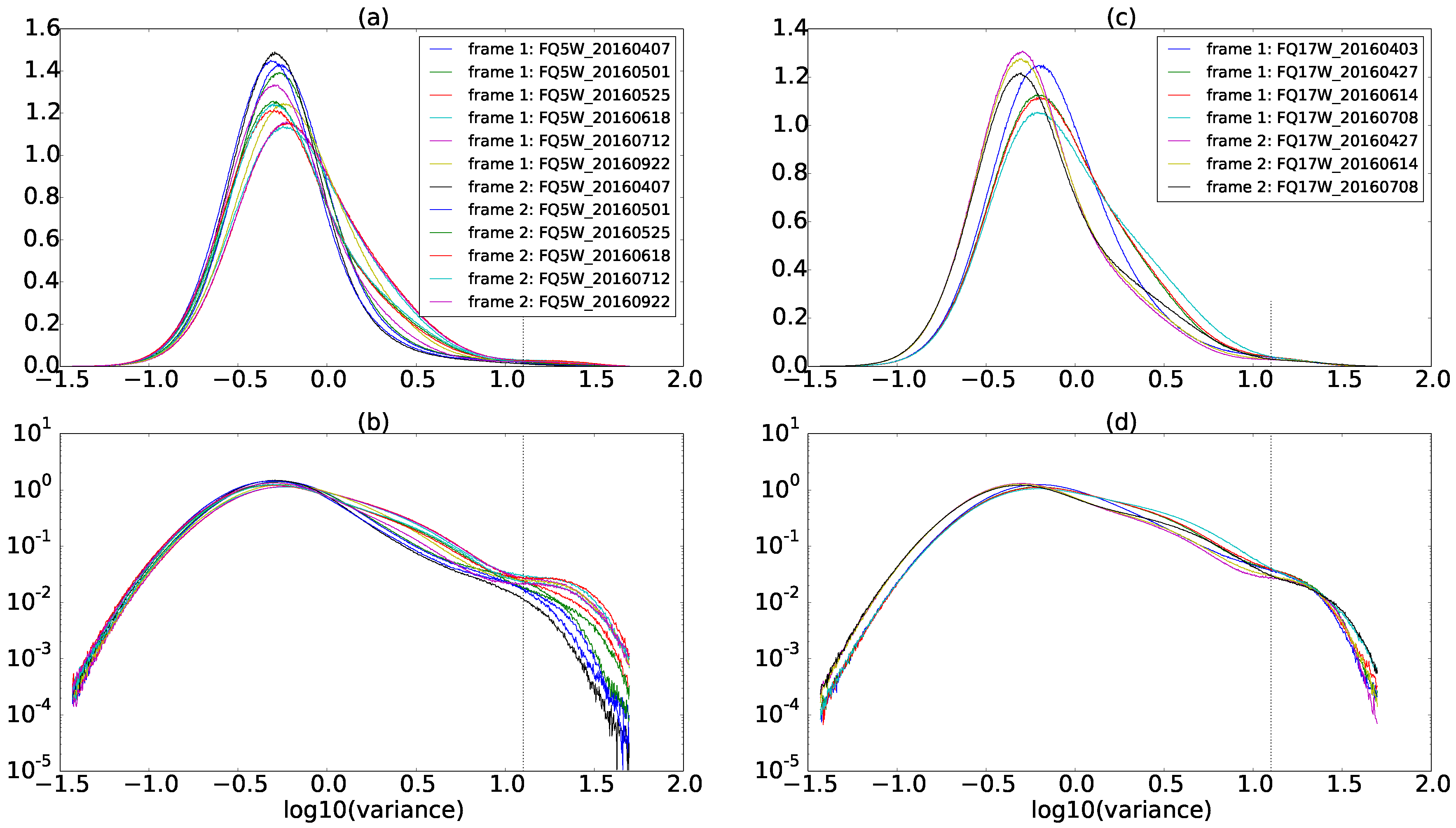
3.2.2. Surface Water Boundary
3.3. Superpixel Segmentation
3.4. Surface Water Extraction
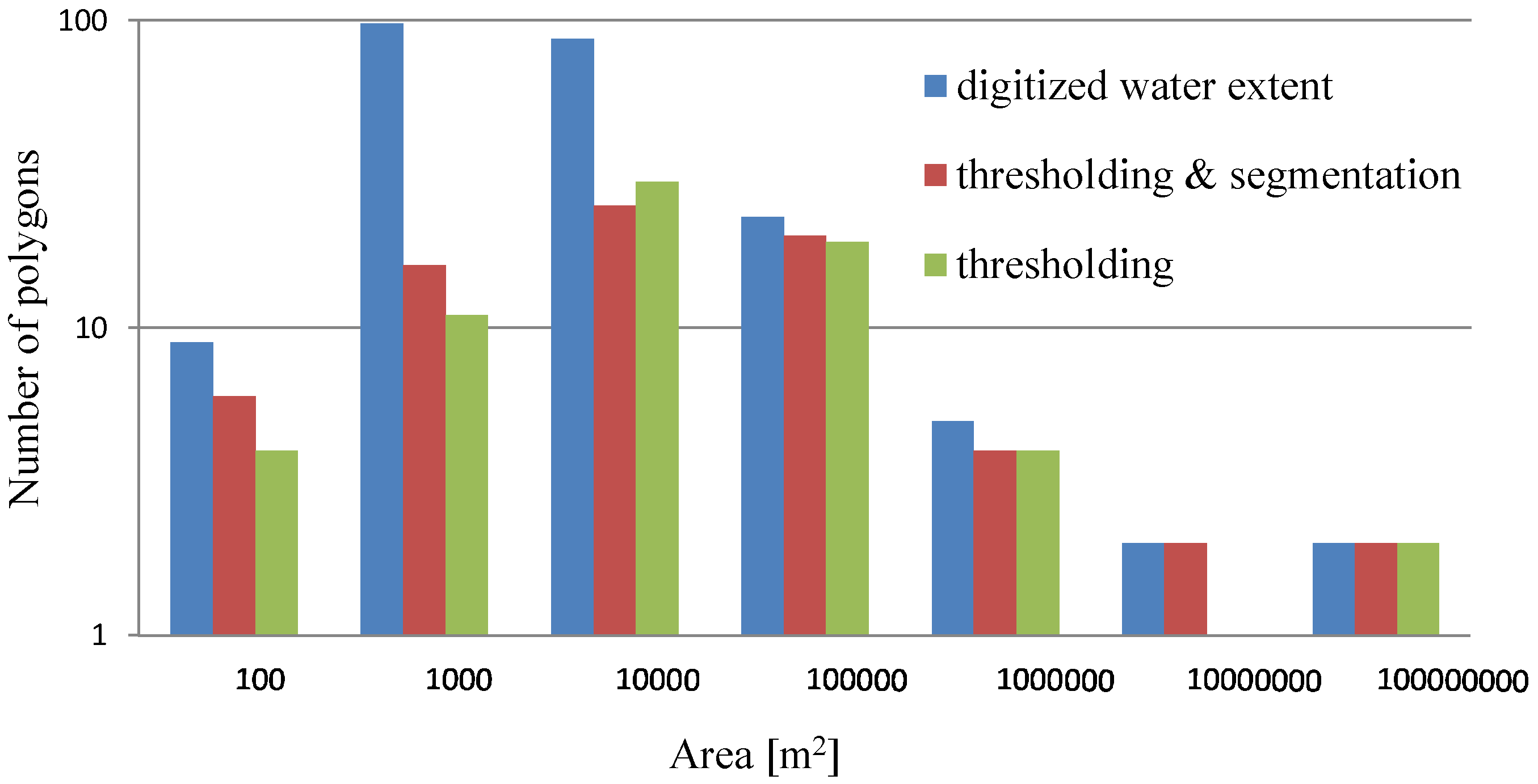
4. Results and Discussion
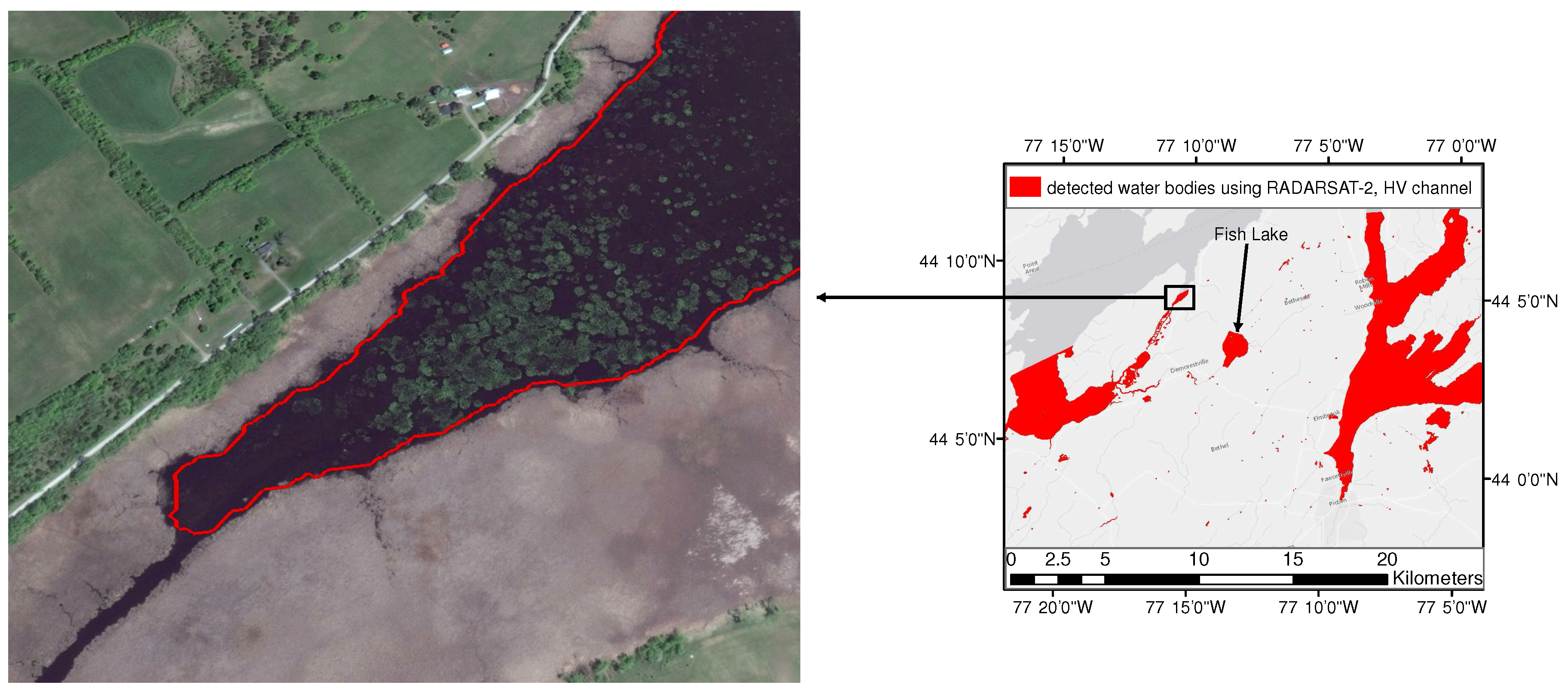
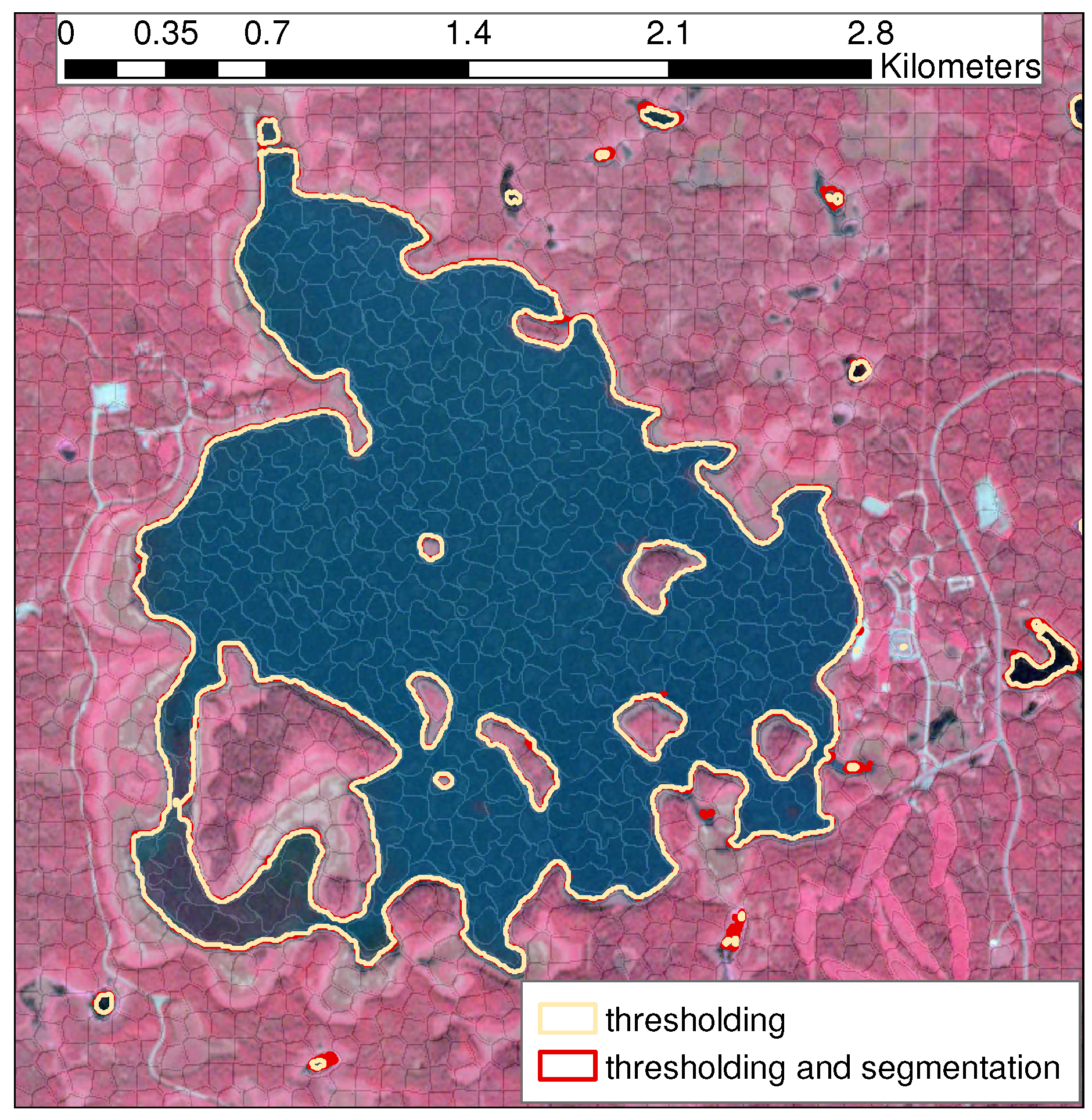
4.1. Bay of Quinte
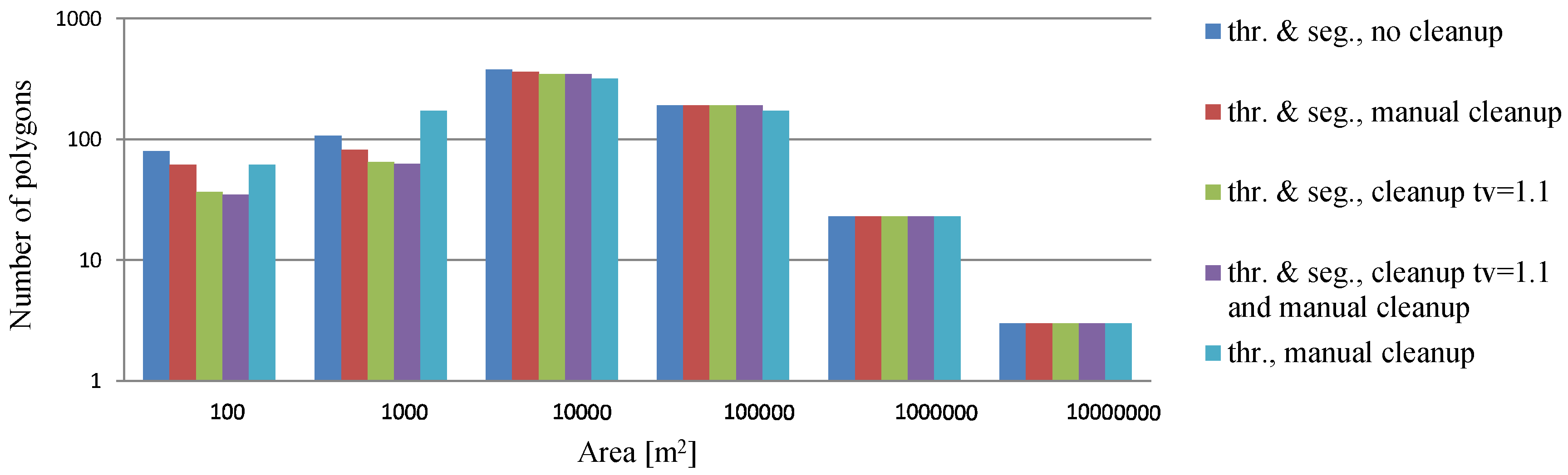
4.2. Prairie Pothole Region
4.3. Limitations and Future Work
5. Conclusions
Acknowledgments
Author Contributions
Conflicts of Interest
Abbreviations
| DEM | Digital Elevation Model |
| ECCC | Environment and Climate Change Canada |
| GCP | Ground Control Point |
| Probability Density Function | |
| RGB | Red, Green, Blue |
| SAR | Synthetic Aperture Radar |
| SLIC | Simple Linear Iterative Clustering |
| SRTM | Shuttle RADAR Topography Mission |
| SWD | Surface Water Detection |
| WVII | WorldView-2 |
Appendix A. Lee Filter and Window Size Effects on Threshold Values

| Window Size | Threshold Value (dB) | Number of Pixels Selected as Water |
|---|---|---|
| 5 × 5 | −26.25 | 861,052 |
| 7 × 7 | −26.02 | 844,465 |
| 9 × 9 | −25.97 | 806,704 |
| 11 × 11 | −25.98 | 770,204 |
References
- Ontario Biodiversity Council (OBC). State of Ontario’s Biodiversity 2010: A Report of the Ontario Biodiversity Council; Ontario Biodiversity Council: Peterborough, ON, Canada, 2010. [Google Scholar]
- Ontario Biodiversity Council (OBC). State of Ontario’s Biodiversity (Web Application); Ontario Biodiversity Council: Peterborough, ON, Canada, 2015. [Google Scholar]
- Stocker, T.F.; Qin, D.; Plattner, G.K.; Tignor, M.; Allen, S.K.; Boschung, J.; Nauels, A.; Xia, Y.; Bex, B.; Midgley, B.M. Climate Change 2013: The Physical Science Basis; Contribution of Working Group I to the Fifth Assessment Report of the Intergovernmental Panel On Climate Change; IPCC: Geneva, Switzerland, 2013. [Google Scholar]
- Desgranges, J.L.; Ingram, J.; Drolet, B.; Morin, J.; Savage, C.; Borcard, D. Modelling wetland bird response to water level changes in the Lake Ontario—St. Lawrence River hydrosystem. Environ. Monit. Assess. 2006, 113, 329–365. [Google Scholar] [CrossRef] [PubMed]
- Doll, P.; Mueller Schmied, H.; Schuh, C.; Portmann, F.T.; Eicker, A. Global-scale assessment of groundwater depletion and related groundwater abstractions: Combining hydrological modeling with information from well observations and GRACE satellites. Water Resour. Res. 2014, 50, 5698–5720. [Google Scholar] [CrossRef]
- Ficke, A.D.; Myrick, C.A.; Hansen, L.J. Potential impacts of global climate change on freshwater fisheries. Rev. Fish Biol. Fish. 2007, 17, 581–613. [Google Scholar] [CrossRef]
- Bolanos, S.; Stiff, D.; Brisco, B.; Pietroniro, A. Technical Note: Operational Surface Water Detection and Monitoring Using Radarsat 2. Remote Sens. 2016, 8, 285. [Google Scholar] [CrossRef]
- Brisco, B.; Short, N.; van der Sanden, J.; Landry, R.; Raymond, D. Technical Note: A semi-automated tool for surface water mapping with RADARSAT-1. Can. J. Remote Sens. 2009, 40, 135–151. [Google Scholar]
- Matgen, P.; Hostache, R.; Schumann, G.; Pfister, L.; Hoffmann, L.; Savenije, H.H.G. Towards an automated SAR-based flood monitoring system: Lessons learned from two case studies. Phys. Chem. Earth 2011, 36, 241–252. [Google Scholar] [CrossRef]
- Li, J.; Wang, S. An automatic method for mapping inland surface waterbodies with Radarsat-2 imagery. Int. J. Remote Sens. 2015, 36, 1367–1368. [Google Scholar] [CrossRef]
- White, L.; Brisco, B.; Pregitzer, M.; Tedford, B.; Boychuk, L. Research Note: RADARSAT-2 Beam Mode Selection for Surface Water and Flooded Vegetation Mapping. Can. J. Remote Sens. 2014, 40, 135–151. [Google Scholar]
- Schumann, G.; Baldassarre, G.D.; Alsdorf, D.; Bates, P.D. Near real-time flood wave approximation on large rivers from space: Application to the River Po, Italy. Water Resour. Res. 2010, 46. [Google Scholar] [CrossRef]
- Otsu, N. A threshold selection method from gray-level histograms. IEEE Trans. Syst. Man Cybern. 1979, 9, 62–66. [Google Scholar] [CrossRef]
- Lee, S.U.; Chung, S.Y.; Park, R.H. A comparative performance study of several global thresholding techniques for segmentation. Comput. Vis. Graph. Image Process. 1990, 52, 171–190. [Google Scholar] [CrossRef]
- Vala, M.H.J.; Baxi, A. A review on Otsu image segmentation algorithm. Int. J. Adv. Res. Comput. Eng. Technol. (IJARCET) 2013, 2, 387–389. [Google Scholar]
- Qin, F.; Guo, J.; Lang, F. Superpixel Segmentation for Polarimetric SAR Imagery Using Local Iterative Clustering. IEEE Geosci. Remote Sens. Lett. 2015, 12, 13–17. [Google Scholar]
- Ren, X.; Malik, J. Learning a Classification Model for Segmentation. In Proceedings of the Ninth IEEE International Conference on Computer Vision, Nice, France, 13–16 October 2003. [Google Scholar]
- Achanta, R.; Shaji, A.; Smith, K.; Lucchi, A.; Fua, P.; Susstrunk, S. SLIC Superpixels; Technical report; EPFL 149300; Images and Visual Representation Laboratory: Lausanne, Switzerland, 2010. [Google Scholar]
- Achanta, R.; Shaji, A.; Smith, K.; Lucchi, A.; Fua, P.; Susstrunk, S. SLIC Superpixels Compared to State-of-the-Art Superpixel Methods. IEEE Trans. Pattern Anal. Mach. Intell. 2012, 34, 2274–2281. [Google Scholar] [CrossRef] [PubMed]
- Ecological Stratification Working Group, Center for Land, Biological Resources Research, State of the Environment Directorate. A National Ecological Framework for Canada; Centre for Land and Biological Resources Research, State of the Environment Directorate: Hull, QC, Canada, 1996. [Google Scholar]
- Canada, E.A. Canadian Climate Normals. Available online: http://climate.weather.gc.ca/climatenormals/ (accessed on 10 October 2017).
- Manjusree, P.; Kumar, L.P.; Bhatt, C.M.; Rao, G.S.; Bhanumurthy, V. Optimization of threshold ranges for rapid flood inundation mapping by evaluating backscatter profiles of high incidence angle SAR images. Int. J. Disaster Risk Sci. 2012, 3, 113–122. [Google Scholar] [CrossRef]
- Martinis, S. Automatic Near Real-Time Flood Detection in High Resolution X-Band Synthetic Aperture Radar Satellite Data Using Context-Based Classification On Irregular Graphs (Doctoral Dissertation, Lmu). Ph.D. thesis, University of Munchen, Bavaria, Geramany, 2010. [Google Scholar]
- Schumann, G.; Hostache, R.; Puech, C.; Hoffmann, L.; Matgen, P.; Pappenberger, F.; Pfister, L. High-resolution 3-D flood information from radar imagery for flood hazard management. IEEE Trans. Geosci. Remote Sens. 2007, 45, 1715–1725. [Google Scholar] [CrossRef]
- Henry, J.B.; Chastanet, P.; Fellah, K.; Desnos, Y.L. Envisat multi-polarized ASAR data for flood mapping. Int. J. Remote Sens. 2006, 27, 1921–1929. [Google Scholar] [CrossRef]
- Mascarenhas, N.D.A. An overview of speckle noise filtering in SAR images. In Proceedings of the First Latino-American Seminar on Radar Remote Sensing, Buenos Aires, Argentina, 2–4 December 1997; Volume 407, p. 71. [Google Scholar]
- Lopes, A.; Touzi, R.; Nezry, E. Adaptive speckle filters and scene heterogeneity. IEEE Trans. Geosci. Remote Sens. 1990, 28, 992–1000. [Google Scholar] [CrossRef]


| Beam | Incident Angle () | Resolution (m) | Orbit Direction | Acquisition Dates in 2016 |
|---|---|---|---|---|
| 7 April, 1 and 25 May, | ||||
| FQ5W | 22.5–26.0 | 13.6–11.9 | Des. | 18 June, 12 July, 22 September |
| FQ17W | 35.7–38.6 | 8.9–8.3 | Asc. | 3 and 27 April, 14 June, 8 July, 25 August |
| FQ5W | FQ17W | |||||||||||
|---|---|---|---|---|---|---|---|---|---|---|---|---|
| Acquisition Date | 7 April | 1 May | 25 May | 18 June | 12 July | 22 September | 3 April | 27 April | 14 June | 8 July | 25 August | |
| Frame 1 | [dB] | −21.71 | −22.52 | −24.31 | −24.15 | −24.20 | −24.47 | −24.57 | −25.07 | −25.06 | −25.84 | −24.71 |
| −0.740 | −0.730 | −0.779 | −0.727 | −0.671 | −0.673 | −1.182 | −1.266 | −1.240 | −1.404 | −1.323 | ||
| Area (only thr.) | 79.144050 | 78.536791 | 90.325668 | 81.645851 | 95.529267 | 77.592698 | 80.108943 | 80.700298 | 80.798277 | 83.484192 | 81.335291 | |
| Area (thr. and seg.; no cleanup) | 78.670027 | 79.046147 | 92.540965 | 83.266778 | 98.375056 | 78.106496 | 80.599210 | 81.973230 | 81.454872 | 84.878121 | 82.414998 | |
| Area (thr. and seg.; cleanup ) | 78.396659 | 78.864226 | 81.436761 | 79.157216 | 83.161622 | 77.032808 | 79.841493 | 79.315489 | 79.291641 | 80.771659 | 79.243893 | |
| Area (thr. and seg.; cleanup manual, ) | 78.129014 | 78.634053 | 77.165192 | 78.042812 | 77.489723 | 76.943957 | 79.213296 | 78.602275 | 78.427127 | 77.792919 | 76.951172 | |
| Frame 2 | [dB] | −21.65 | −22.68 | −24.10 | −24.05 | −24.05 | −23.25 | −24.45 | −24.59 | −24.73 | ||
| −0.208 | −0.199 | −0.154 | −0.138 | −0.078 | −0.141 | −0.302 | −0.300 | −0.297 | ||||
| Area (only thr.) | 78.413984 | 78.405075 | 90.819369 | 82.320027 | 96.334413 | 78.040422 | 82.606517 | 80.857515 | 85.732206 | |||
| Area (thr. and seg.; no cleanup) | 78.854678 | 79.215934 | 92.954831 | 84.087752 | 96.568122 | 78.652638 | 83.322545 | 82.294253 | 87.964080 | |||
| Area (thr. and seg.; cleanup ) | 78.576186 | 79.389975 | 81.886128 | 79.532122 | 84.675813 | 77.146079 | 79.654046 | 79.755364 | 83.387152 | |||
| Area (thr. and seg.; cleanup manual, ) | 78.2574461 | 78.771559 | 77.197498 | 78.124867 | 77.612345 | 77.051342 | 78.790877 | 78.472412 | 78.043980 | |||
| Frame No. | Acquisition Date | 3 April | 27 April | 14 June | 8 July | 25 August |
|---|---|---|---|---|---|---|
| thr. and seg.; no cleanup | 1.7 | 4.3 | 3.9 | 9.1 | 7.1 | |
| thr. and seg.; cleanup, | 0.9 | 1.5 | 1.3 | 5.6 | 4.1 | |
| Frame 1 | thr. and seg.; cleanup, | 0.8 | 0.9 | 1.1 | 3.8 | 3.0 |
| thr. and seg.; cleanup, | 0.7 | 0.5 | 0.6 | 2.3 | 1.9 | |
| thr. and seg.; cleanup, | 0.5 | 0.2 | 0.3 | 1.3 | 0.8 | |
| thr. and seg.; no cleanup | 5.7 | 4.9 | 12.7 | |||
| thr. and seg.; cleanup, | 1.7 | 2.0 | 8.9 | |||
| Frame 2 | thr. and seg.; cleanup, | 1.1 | 1.6 | 6.8 | ||
| thr. and seg.; cleanup, | 0.4 | 1.0 | 3.8 | |||
| thr. and seg.; cleanup, | 0.03 | 0.6 | 2.4 | |||
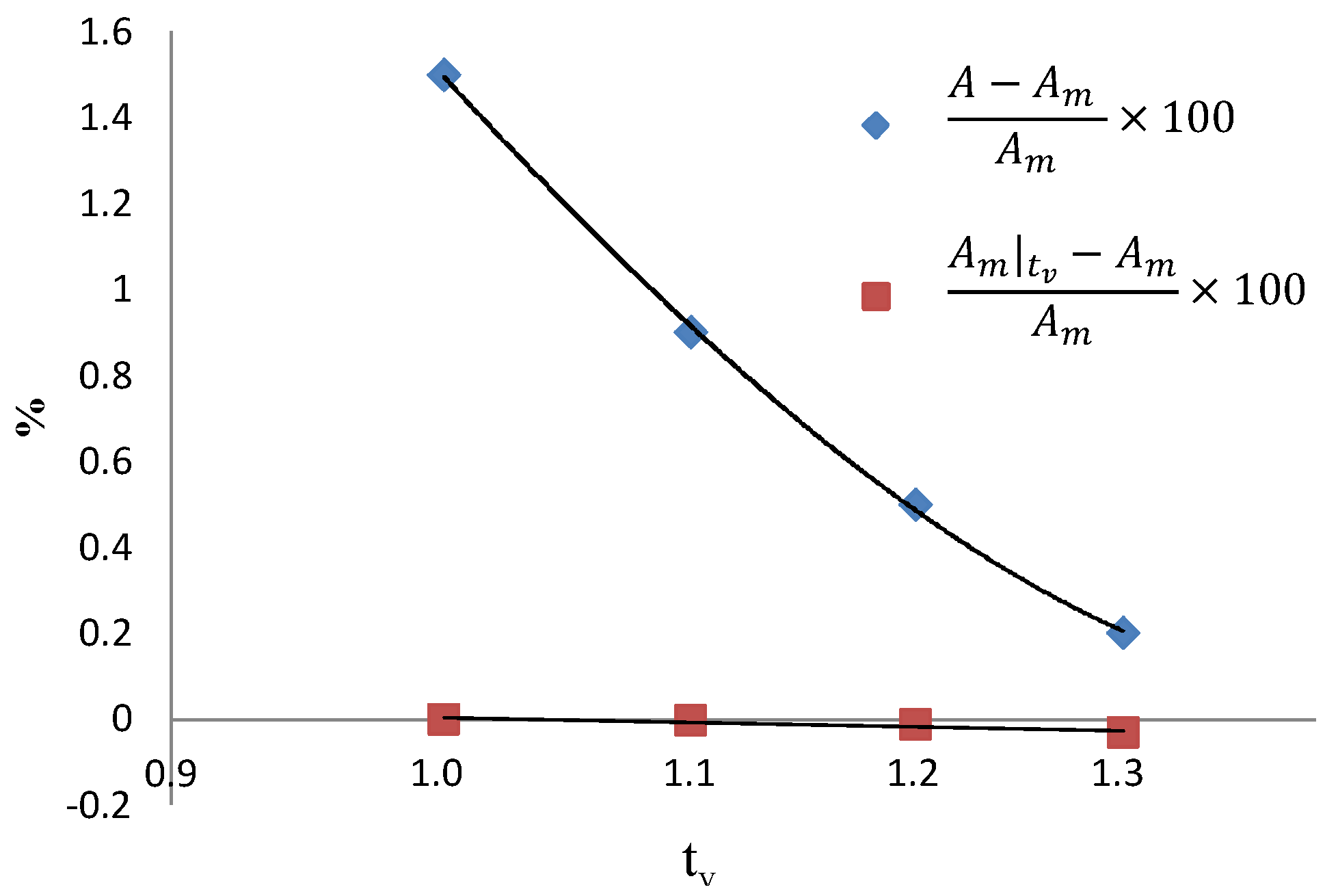
| Frame No. | Acquisition Date (27 April) | No. of Polygons | (km) | Largest Lost Polyg. (m) | |
|---|---|---|---|---|---|
| Frame 1 | thr. and seg.; manual cleanup | 81 | 78.602275 | 0.0000 | |
| thr. and seg.; cleanup, | 78 | 78.601957 | −0.0004 | 149 | |
| thr. and seg.; cleanup, | 75 | 78.600120 | −0.0027 | 1077 | |
| thr. and seg.; cleanup, | 71 | 78.593149 | −0.0116 | 6232 | |
| thr. and seg.; cleanup, | 66 | 78.576692 | −0.0325 | 11809 | |
| thr. ; manual cleanup | 72 | 78.052080 | −0.7000 | 1288 |
| Frame No. | Fish Lake Acquisition Date (27 April) | Total Area | Underestimated Area | Overestimated Area |
|---|---|---|---|---|
| digitized water extent | 1,608,511 | 0 | 0 | |
| Frame 1 | thresholding and segmentation | 1,574,172 | 38,447 | 4192 |
| thresholding | 1,553,469 | 56,220 | 1261 |
| Region | Acquisition Date (8 September 2012) | No. of Polygons | Detected Surface Water (km) |
|---|---|---|---|
| Prairie Potholes | thr. and seg.; no cleanup | 785 | 20.168476 |
| thr. and seg.; manual cleanup | 698 | 20.100138 | |
| thr. and seg.; cleanup | 669 | 20.073126 | |
| thr. and seg.; cleanup and manual cleanup | 662 | 20.065713 | |
| thr.; manual cleanup | 755 | 19.044606 |
© 2017 by the authors. Licensee MDPI, Basel, Switzerland. This article is an open access article distributed under the terms and conditions of the Creative Commons Attribution (CC BY) license (http://creativecommons.org/licenses/by/4.0/).
Share and Cite
Behnamian, A.; Banks, S.; White, L.; Brisco, B.; Millard, K.; Pasher, J.; Chen, Z.; Duffe, J.; Bourgeau-Chavez, L.; Battaglia, M. Semi-Automated Surface Water Detection with Synthetic Aperture Radar Data: A Wetland Case Study. Remote Sens. 2017, 9, 1209. https://doi.org/10.3390/rs9121209
Behnamian A, Banks S, White L, Brisco B, Millard K, Pasher J, Chen Z, Duffe J, Bourgeau-Chavez L, Battaglia M. Semi-Automated Surface Water Detection with Synthetic Aperture Radar Data: A Wetland Case Study. Remote Sensing. 2017; 9(12):1209. https://doi.org/10.3390/rs9121209
Chicago/Turabian StyleBehnamian, Amir, Sarah Banks, Lori White, Brian Brisco, Koreen Millard, Jon Pasher, Zhaohua Chen, Jason Duffe, Laura Bourgeau-Chavez, and Michael Battaglia. 2017. "Semi-Automated Surface Water Detection with Synthetic Aperture Radar Data: A Wetland Case Study" Remote Sensing 9, no. 12: 1209. https://doi.org/10.3390/rs9121209