Online Global Land Surface Temperature Estimation from Landsat


1
Remote Sensing Lab, Institute of Applied and Computational Mathematics, Foundation for Research and Technology Hellas (FORTH), N. Plastira 100, Vassilika Vouton, 70013 Heraklion, Greece
2
Jet Propulsion Laboratory, California Institute of Technology, MS 183-501, 4800 Oak Grove Drive, Pasadena, CA 91109, USA
*
Author to whom correspondence should be addressed.
Remote Sens. 2017, 9(12), 1208; https://doi.org/10.3390/rs9121208
Submission received: 29 September 2017
/
Revised: 15 November 2017
/
Accepted: 15 November 2017
/
Published: 23 November 2017
(This article belongs to the Special Issue Remote Sensing for Land Surface Temperature (LST) Estimation, Generation, and Analysis)
Abstract
:This study explores the estimation of land surface temperature (LST) for the globe from Landsat 5, 7 and 8 thermal infrared sensors, using different surface emissivity sources. A single channel algorithm is used for consistency among the estimated LST products, whereas the option of using emissivity from different sources provides flexibility for the algorithm’s implementation to any area of interest. The Google Earth Engine (GEE), an advanced earth science data and analysis platform, allows the estimation of LST products for the globe, covering the time period from 1984 to present. To evaluate the method, the estimated LST products were compared against two reference datasets: (a) LST products derived from ASTER (Advanced Spaceborne Thermal Emission and Reflection Radiometer), as higher-level products based on the temperature-emissivity separation approach; (b) Landsat LST data that have been independently produced, using different approaches. An overall RMSE (root mean square error) of 1.52 °C was observed and it was confirmed that the accuracy of the LST product is dependent on the emissivity; different emissivity sources provided different LST accuracies, depending on the surface cover. The LST products, for the full Landsat 5, 7 and 8 archives, are estimated “on-the-fly” and are available on-line via a web application.

1. Introduction
Land surface temperature (LST) is an important parameter for environmental studies and enables the monitoring of landscape processes and responses [1], such as the surface energy and water balance [2,3,4,5,6,7]. In order to better observe the changes, in climate for example, there is a need for frequent data acquisition to obtain consistent LST time series [8]. Especially at the regional [9] and global scales, the only way to study the surface temperature is with satellite monitoring [10].
The Landsat 5, 7 and 8 satellites carry thermal infrared radiometers and therefore their data are suitable for LST estimation. During the last decades, there is an increasing demand for satellite-derived surface temperature products, to be used in various studies and applications. Landsat-derived LST is widely used for urban temperature studies and particularly for the study of the urban heat island (UHI) phenomenon [11,12,13]. Recently, LST data from Landsat were used for urban energy flux estimation [3]. Landsat-derived LST is also used for monitoring the forested areas, such as the correlation of LST with tree loss or the detection of changes in tropical forest cover [14,15]. The land cover/use changes affect LST as well, as has been demonstrated in different studies, using different types of satellite data [16].
A large number of studies present different algorithms and approaches for LST retrieval from Landsat [17,18,19,20]. Some of these algorithms have also been implemented in software tools. For example, a plugin for the open-source software QGIS [21] calculates LST from Landsat 5, 7 and 8 imagery [22]. Similar tools have been developed for ERDAS [23] software, for processing Landsat 8 thermal acquisitions [24]. However, such tools require software installation and, most importantly, raw satellite data downloads, which can be extremely time-consuming. It should be noted that the U.S. (United States) Geological Survey (USGS) has announced the release of LST products from the full Landsat archive, but these products are not yet available [25].
The objective of this work is to describe a method implemented in a web application, specifically developed to provide fast and easy access to LST for the globe from the Landsat archive. The approach uses a single channel (SC) algorithm [19,20] to analyse Landsat 5, 7 and 8 thermal infrared observations. It is noted that SC approaches are not as efficient as split-window approaches [20,26], but are necessary for satellites acquiring with only one thermal band, like Landsat 5 and 7. Three different sources of emissivity were considered to allow more accurate LST estimates for different regions and conditions: a global emissivity map derived from ASTER (Advanced Spaceborne Thermal Emission and Reflection Radiometer) data, that refers to the period 2000–2008 and is at 100 m × 100 m spatial resolution [27,28]; the MODIS (Moderate Resolution Imaging Spectroradiometer) daily LST/emissivity product at 1 km × 1 km spatial resolution [29]; and emissivity based on the vegetation fraction estimated from NDVI (Normalized Difference Vegetation Index) [30].
The number of studies that use LST is growing, and satellites may provide accurate and up-to-date LST products. Providing easy access to accurate, global and up-to-date LST data is expected to benefit a large number of studies. In the era of information technology, this ever-growing demand for LST data opens the path for new unexplored ways of distributing big data information through web applications. Using online platforms, like the Google Earth Engine (GEE) [31], with access to a huge catalogue of satellite imagery and planetary-scale analysis capabilities, it is now possible to build web applications that do not require any pre-processing or installation of software. An application of this type, capable of “on-the-fly” LST estimation from Landsat thermal infrared observations, for any given geographical area and date range, has been developed and presented in this study. The LST estimation process is performed in the background on the Google cloud computing servers, with direct access to the GEE satellite data catalogue. Therefore, the application needs only a few seconds to produce Landsat LST with no need for any computational resources from the user.
The following section outlines the theoretical basis of the SC methodology, describes the data used for the LST estimation, including the different emissivity sources, describes the algorithm implementation in GEE and the products accuracy assessment approach. In the following, the effect of using different parameterizations of the SC algorithms are discussed and a quantitative analysis is presented, along with the accuracy assessment results. Finally, the web application interface is presented and followed by the conclusion of this study.
2. Materials and Methods
2.1. LST Algorithm
SC is a commonly-used approach to estimate LST from the Landsat thermal infrared observations [19,20,32,33]. Among Landsat 5, 7 and 8, only Landsat 8 carries two thermal bands [34], therefore the SC approach is used in this study for consistency. Table 1 presents the wavelength range and the spatial resolution of each Landsat thermal band, along with the time period of operation. The SC algorithm needs surface emissivity information from external sources.
Using an SC approach, the LST (TS) can be calculated from the radiance-at-the-sensor in a single band using the radiative transfer equation in the following form:
where B is the Planck function, Lsen is the radiance-at-the-sensor, Lup is the thermal path radiance, Ldown is the downwelling irradiance, ε is the surface emissivity and τ is the atmospheric transmissivity.
In Equation (1) the Lup, Ldown and τ need to be known for the specific area for which we calculate the LST. These variables make the process of establishing a single global LST algorithm extremely difficult, since they are prone to changes, and bound only to the area under study [19,20]. They are also heavily dependent on the total water vapour in an atmospheric column (precipitable water (PW)), which is also easier to determine with the use of satellite data as [37]. Jimenez-Munoz et al. [19,20] developed a methodology that uses coefficient tables through simulations with many different atmospheric profile inputs, capable of parameterizing the local transmissivity, path radiance and downwelling irradiance, to lead to one equation that is more convenient to use on a global scale LST calculation. In this study, LST is estimated using the approach proposed by Jimenez-Munoz et al. [19,20]:
where:
where Planck’s constant value is 1.19104 × 10⁸ W μm4 m−2 sr−1 and is 14,387.7 μm K; λ is the central wavelength of the thermal band of the Landsat sensor in question; Lsen in W sr−1 m−2 μm−1; Tb is the brightness temperature in Kelvin; C is the coefficients table, with cij derived by simulations using different atmospheric profiles [19,20]; and ψx is the coefficients weighted with PW. The various datasets that are used in this study to estimate LST from Equation (2) are described in detail below.
2.2. Data Used for LST Estimation
The main source of data in this study concerns Landsat 5, 7 and 8 acquisitions, provided by the USGS and included in the GEE data catalogue. GEE provides easy and instant access to satellite products and the computing resources to process them directly on the platform, with no need for download. Data from the different sources and satellites are organized in image collections that make their combination and simultaneous processing feasible. Table 2 presents the data used for LST estimation along with their GEE data catalogue identifier. Short explanations of each product are given below.
2.2.1. Landsat Thermal Radiance-at-Sensor
The level 1T (precision Ortho-corrected) products for each Landsat, provided by the USGS, are orthorectified images of the thermal infrared radiance-at-the-sensor. These products are available in the form of an image collection for each Landsat in the GEE catalogue. The images in the different collections contain digital number values, which are converted to radiance-at-sensor via a GEE function using scaling factors. Although the Landsat thermal bands are of different spatial resolutions (Table 1), there is consistency among different Landsat sensors, since all the products are resampled by the USGS to 30 m × 30 m, using a cubic convolution resampling method [35,36].
2.2.2. Brightness Temperature and Cloud Mask
Although the brightness temperature can be easily estimated by directly inverting the Planck function, the GEE catalogue includes an image collection of Landsat top-of-the-atmosphere (TOA) brightness temperature. The Landsat brightness temperature product in the GEE catalogue contains cloud cover information derived by the Fmask approach [38,39]. Fmask is a method for detecting among others, clouds, cloud shadows and water surfaces in Landsat imagery. The brightness temperature and information on the clouds, cloud shadows and water surfaces was used in this study from these image collections.
2.2.3. Landsat Surface Reflectance
The Landsat Surface Reflectance is a higher-level product of surface reflectance information for six bands (0.25–2.35 μm) at 30 m × 30 m spatial resolution, generated by LEDAPS (Landsat Ecosystem Disturbance Adaptive Processing System) and distributed by the USGS [40]. The Landsat surface reflectance is available through the GEE catalogue, in the form of image collections. The red and near-infrared bands are used for the calculation of the NDVI, which is needed in order to estimate the NDVI-based emissivity in the present study.
2.2.4. Emissivity
Emissivity is a critical variable for the LST estimation, since a small uncertainty in the emissivity (1%) can lead to large errors in the LST (up to 1 K) depending on the setting of the sensor, the climatological conditions and geographical setting of the area [41,42]. In this study, three different sources of emissivity are used: ASTER and MODIS emissivity that are available in the GEE catalogue and NDVI-based emissivity estimated from Landsat red and near-infrared data. The reason for using a variety of emissivity sources is to test their strengths and weaknesses, by comparing their impact on the LST retrieval for different land cover types, corresponding to different landscapes and ecosystems. Table 3 summarizes the different emissivity sources used in this study.
The MODIS/Terra Land Surface Temperature and Emissivity products (MOD11A1) provide per-pixel temperature and emissivity values in a sequence of swath-based to grid-based global products. This is a tile-based and gridded level three product produced daily at 1 km × 1 km spatial resolution. The surface emissivities in bands 31 and 32 are estimated from land cover types [43,44]. The average emissivity value of bands 31 and 32 is used in this study. Nearest neighbour resampling is used to match the Landsat spatial resolution.
The ASTER Global Emissivity Database (ASTER-GED) was developed by JPL (Jet Propulsion Laboratory). This product is derived from clear-sky pixels for available ASTER data between 2000 and 2008, covering the globe. It has a (nominal) spatial resolution of 100 m × 100 m and includes, among others, the mean emissivity and standard deviation for all five ASTER thermal infrared bands separately from all the clear pixels during the 2000–2008 period. The emissivity value of band 14 (10.95–11.65 μm) is used in this study. Nearest neighbour resampling is used to match the Landsat spatial resolution.
NDVI-based emissivity is estimated from the Landsat visible and near-infrared bands and typical emissivity values, following the approach described in [30]. The fraction of vegetation cover (FVC) [30] is estimated using Equation (6), by assuming the NDVI threshold for non-vegetated (NDVInonveg) and vegetated (NDVIveg) surfaces to be 0.18 and 0.85, respectively [19]. Finally, the emissivity is estimated using Equation (7), assuming a reference emissivity for non-vegetated (εnonveg) and vegetated surfaces (εveg) to be 0.97 and 0.99, respectively [19].
The NDVI-based emissivity product is of 30 m × 30 m spatial resolution, matching exactly the Landsat thermal data.
2.2.5. Atmospheric PW Content
Information on PW is necessary for the atmospheric correction of thermal observations. The atmospheric correction is indirectly performed in Equation (2). The NCEP/NCAR (National Centers for Environmental Prediction/National Centre for Atmospheric Research) reanalysis project data have among others, PW values of six-hour temporal resolution (00:00, 06:00, 12:00 and 18:00 UTC) and 2.5-degree spatial resolution [45]. The GEE product comes as an image collection of PW. In order to align the NCEP/NCAR reanalysis PW product with the Landsat imagery in this study, a time adjustment was necessary in order to choose for each day the PW product that is representative for the Landsat acquisition time. This is achieved through the timestamps in the metadata of every image and by estimating the average PW between the two PW values, which are close in time. It is worth noting that the atmospheric PW content can also be estimated with the use of satellite data [37,46]. The MODIS PW product for example could be used instead of the NCEP/NCAR reanalysis, but this product is not yet available in the GEE catalogue.
2.2.6. Coefficient Tables for Atmospheric Parameterization
Different coefficient tables, in Equation (5), are obtained through simulations with many different atmospheric sounding inputs [19]. These are created with atmospheric profiles for different locations all over the world. For Landsat 5 and 7, five coefficient tables are available, created using five different databases of atmospheric soundings and MODTRAN code [19]: a custom database named STD (six standard) constructed with data from six standard atmospheric profiles (tropical, midlatitude summer, midlatitude winter, subartic summer, subartic winter and U.S. Standard); three databases, TIGR1, TIGR2, TIGR3 (thermodynamic initial guess retrieval), with TIGR1 being a reduced version of the original TIGR1, TIGR2 being an extension of the original TIGR1 and TIGR3 an extension of TIGR2; and SAFREE, a combination of TIGR1, TIGR2 and radiosondes from Meteo France and the Norwegian Meteorological services. For Landsat 8 only one coefficient table was available [20], corresponding to the GAPRI (Global Atmospheric Profiles from Reanalysis Information) database by the ERA-interim (European Reanalysis) reanalysis data [47].
2.3. LST Algorithm Implementation in the GEE
The algorithm described in Section 2.1 is implemented in the GEE using the data described in Section 2.2. GEE has two APIs (application programming interfaces), a JavaScript and a Python interface. Both provide libraries of functions for accessing Google’s computing and storage infrastructure. The JavaScript API is used through ‘playground’, which is the web-based IDE (integrated development environment) of GEE. The ‘playground’ provides a ready-to-use editor to test the code and easily see the results. An issue with the GEE ‘playground’ is that it provides limited access through invitation, and thus it is not suitable for open-access application development. The Python API provides the same functionalities and follows the same principles as the JavaScript API. The main difference, besides the programming language, is that the Python API can be used to develop custom web applications accessible by everyone. The SC method described in Section 2.1 was first implemented in the GEE’s ‘playground’ for easy testing. Once operational, the JavaScript code was translated into Python and a web application was developed using the Google App Engine. The application is accessible to everyone and a user-friendly environment allows easy access to the Landsat LST products.
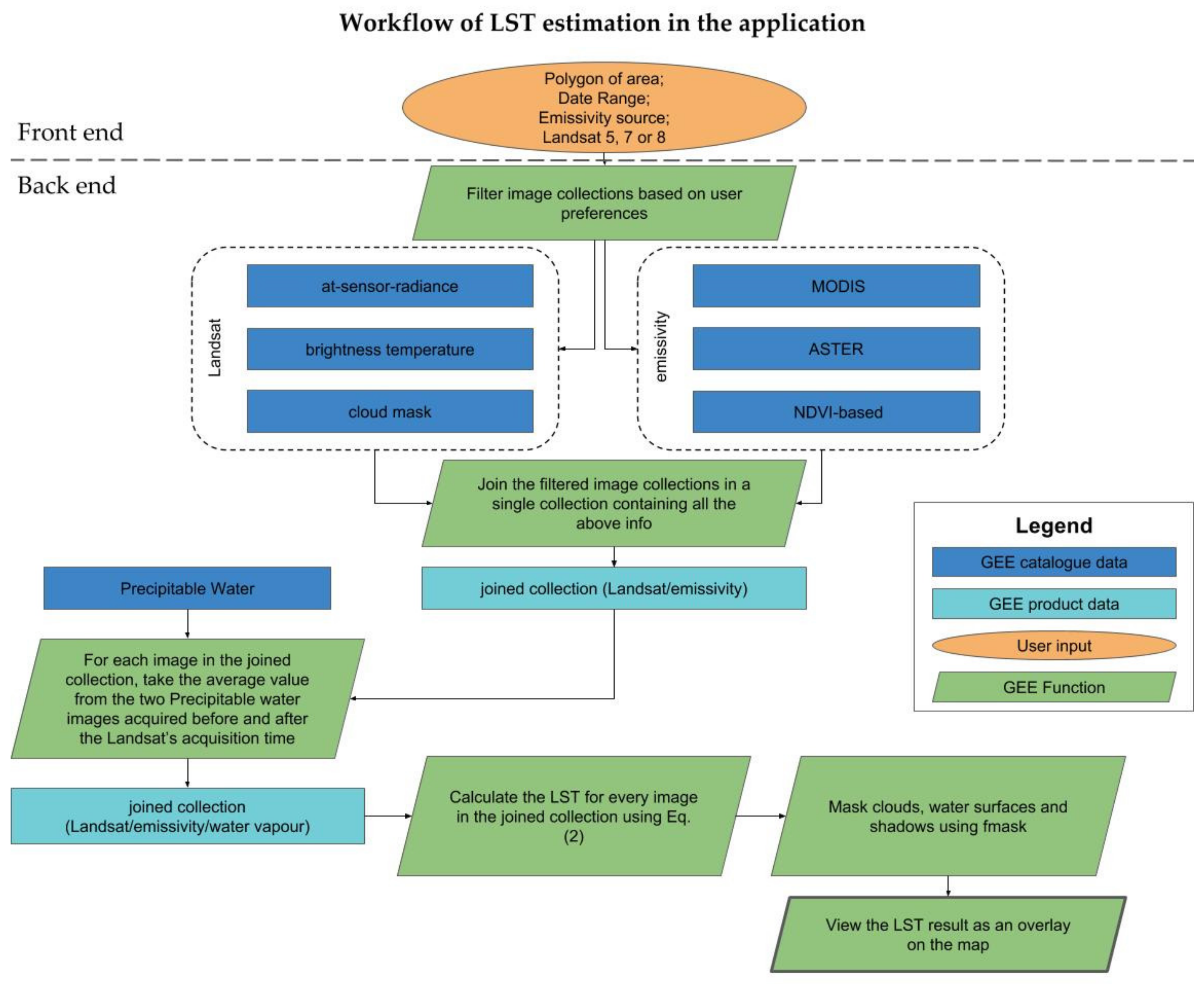
Figure 1 graphically illustrates the implementation algorithm and the flow of data in the application. Initially, the user draws a polygon on the map to mark the area of interest and provides information on the preferred date range, emissivity source (ASTER, MODIS or NDVI) and Landsat satellite (5, 7 or 8). These choices are made in the front end of the application in an interactive environment. Then an AJAX (Asynchronous JavaScript and XML (extensible markup language)) request containing the user’s preferences is sent to the back end of the application and more specifically to the Python API which provides access to the GEE product catalogue and functions. The selected Landsat radiance and brightness temperature image collections are then accessed and filtered for the required geographical area and date range. For MODIS emissivity, a filter for the selected area and date range is applied, since the MODIS emissivity product is daily. For ASTER emissivity, only the area filter is applied, since there is only one emissivity map corresponding to 2000–2008. For the NDVI-based emissivity, calculations need to be performed. A filter is applied to the Landsat surface reflectance product for the date and area and then calculates the emissivity as described in Section 2.2.4. The different image collections (the radiance, brightness temperature with cloud mask and emissivity) are then joined in a single image collection. The PW data is handled differently than other image collections, since it has a 6-h temporal resolution. First the PW collection is filtered for the selected area and date range. Then the average of the two PW values is selected, the first value is the PW that was acquired closest in time before the Landsat image and second is that acquired closest after the Landsat image. The PW is added using this methodology to every image in the joined collection which now contains all the necessary data for the LST estimation of the specific geographical area and date range. It is worth noting the flexibility of GEE to easily combine all the satellite data products from different sources and of different spatial resolutions, using the nearest neighbour resampling method (or other method if requested). Equation (2) is then applied to every image in the joined collection to estimate the LST products for the selected area and date range. The water surfaces, clouds and shadows are removed from the LST products in the final steps by using the Fmask (Section 2.2.2). In the end, the Python API requests from the GEE a download link and a map layer from Google Maps to visually represent every image. The AJAX request returns to the front end with that information so both the visualization and download functions are available to the users for the calculated Landsat LST products.
2.4. Accuracy Assesment
Since validation with in-situ data was beyond the scope of this study and since at the time of the study other operational Landsat LST products were not available for comparison, the accuracy assessment of the LST products was based on indirect verification. Thus, ASTER higher-level LST products [48] were considered as a reference dataset to assess the accuracy of the Landsat-derived LST. ASTER LST products were selected for their high accuracy, which is reported to be of 1.5 K [49]. A thorough analysis of ASTER radiance and temperature accuracies is reported in [50]. Using instrumented buoys in large lakes, for 246 independent validations of surface temperature, they reported that all channels were well within the preflight specification of ±1 K. Comparing a dynamically changing variable such as the surface temperature derived from different satellites is challenging. In this study, a time difference of maximum half an hour is allowed, therefore, ASTER LST products were compared to Landsat 7 LST products. The LST derived from Landsat 5 and 8 in GEE was evaluated by comparison with other Landsat 5- and 8-derived LST from the same observations, but using alternative approaches, such as the approach implemented by the software ATCOR [51]. GEE was used for selecting ASTER images that meet the reference data selection criteria. Using the GEE catalogue was very efficient in matching the acquisition dates of ASTER and Landsat 7 with time differences of less than half an hour. From the resulting matching Landsat and ASTER image pairs, a number of pairs was manually selected to cover different geographic areas around the world, with distinguishable surface cover (desert, dense forest, cities, etc.). Images corresponding to different seasons and a large range of PW values were selected, to ensure testing for a variety of different atmospheric conditions. For the selected dates, the ASTER LST products were provided by JPL (Jet Propulsion Laboratory). For Landsat 5 and 8, no ASTER data with a time difference of less than half an hour in acquisition time were available. Thus, a set of Landsat 5 and 8 LST products estimated with ATCOR for the cities of Heraklion and Basel were used, that were produced by the DLR (German Aerospace Agency). All the reference images that were used are listed in Table 4 with their acquisition date, spatial resolution, a reference point of the location, area size and PW values.
The comparison process includes the estimation of the Landsat LST as described in Section 2.1, for 13 images, using all combinations of the three emissivity sources, the five coefficient tables for Landsat 5 and 7 and one coefficient table for Landsat 8. In total, 147 Landsat LST products were available for comparison. Post-processing was necessary for the LST product derived by Landsat 7 in order to be comparable to the ASTER LST products, mainly due to their different spatial resolution. The Landsat LST products at 30 m × 30 m spatial resolution were resampled to 90 m × 90 m, using spatial averaging. The RMSE (root mean square error) was used as an accuracy metric in all cases.
3. Results and Discussion
3.1. Accuracy Assesment
The accuracy of the Landsat LST products was assessed as explained in detail in Section 2.4, based on indirect validation with ASTER and Landsat LST products, derived using different approaches. The set of 147 Landsat LST products was compared to the reference data and the accuracy assessment results for different coefficient tables and emissivity sources are presented and discussed below.
3.1.1. Atmospheric Effects: Coefficient Table Comparisons
The first accuracy test concerns a comparison among LST products estimated based on different coefficient tables. The objective was to assess the magnitude of errors for the different areas tested and to select one model to be used in the GEE implementation. Figure 2 shows the RMSE using different coefficient tables for Landsat 5 and Landsat 7. No results are presented for Landsat 8 since only one coefficient table was available (see Section 2.2.6). For Landsat 5, the use of the SAFREE coefficient table resulted in lower RMSE, with an average value of 1.49 °C (bias −0.54), while TIGR3 was very close with an average RMSE of 1.50 °C (bias −0.64). For Landsat 7, TIGR2 performed better than the other coefficient table with an average RMSE of 1.77 °C (bias 0.9). The reference data had a variety of PW ranging from 0.72 to 4.32 g/cm2. Our results are in line with [19], where for a PW range between 0.5 and 3 g/cm2 the best RMSE was obtained by using the STD, TIGR2 and SAFREE databases.
Consequently, the coefficient table corresponding to SAFREE was adopted in the final methodology for Landsat 5, the TIGR2 for Landsat 7 and the GAPRI for Landsat 8, as it was the only one available at the time.
3.1.2. Emissivity Effects: Comparisons of the Different Emissivity Retrieval Methods
As already mentioned, three emissivity data sources were used in the LST estimation: the ASTER-GED, the daily MODIS emissivity product and NDVI-based emissivity. This allowed the assessment of the emissivity impact on the LST. The reference data were split into two main categories based on the surface cover of the area: natural/isolated landscapes and urban/peri-urban areas. The first category includes areas that are not much affected by human activity and they do not exhibit vast changes over time. In practise, this category includes images from the Amazon forest, the West Virginia Mountains and the Sahara Desert (Table 4). The second category includes images of cities (Table 4) and the surface cover of the areas depicted in the images are, thus, affected by human activity. Figure 3 shows the RSME of the estimated LST compared to the reference data for each of the two main categories and for each emissivity source. The emissivity of natural/isolated landscapes is not expected to present significant changes over time, since the land cover does not change; in contrast, human activity, particularly urbanization and agricultural activities, are responsible for intense land cover changes, which impact emissivity. As thus expected, the ASTER emissivity provides more accurate LST estimates for the natural/isolated landscapes (average RMSE of 1.54 °C, bias 0.66) than MODIS and NDVI-based emissivity. For the urban/peri-urban areas on the other hand, all emissivity sources provide very similar results in terms of LST error. The reason is that these are highly heterogeneous and mixed areas in space.
Overall, from Figure 3, it seems that the ASTER emissivity provides slightly better results, despite the fact that it is a single static image compared to the other frequently-updated emissivity options. This can be explained by the high quality of ASTER products compared to the other emissivity options, in the areas where the average emissivity remains similar, the values from the static ASTER image are still relevant. On the other hand, in urban/peri-urban areas, where land cover/use changes continuously and alters emissivity’s spatial distribution, the more frequent emissivity retrievals from MODIS and NDVI seem to be on par with ASTER accuracy. For future estimations of LST that are far in time from the 2000–2008 ASTER emissivity map, this gap will probably increase and the ASTER emissivity data will become outdated.
The NDVI-based emissivity maps have a better spatial resolution (30 m × 30 m) than the MODIS-maps (1 km × 1 km), while in terms of temporal resolution both products refer to the Landsat acquisition time. For the NDVI-based emissivity, the NDVInonveg and NDVIveg in Equation (6) have fixed values of 0.18 and 0.85 instead of being estimated particularly for each region. In a global study, the terrain is very much diverse in different areas and these NDVI fixed values are not fully representative for all situations. This possibly explains the slightly poor performance of NDVI-based emissivity compared to the MODIS emissivity in the Landsat LST estimation.
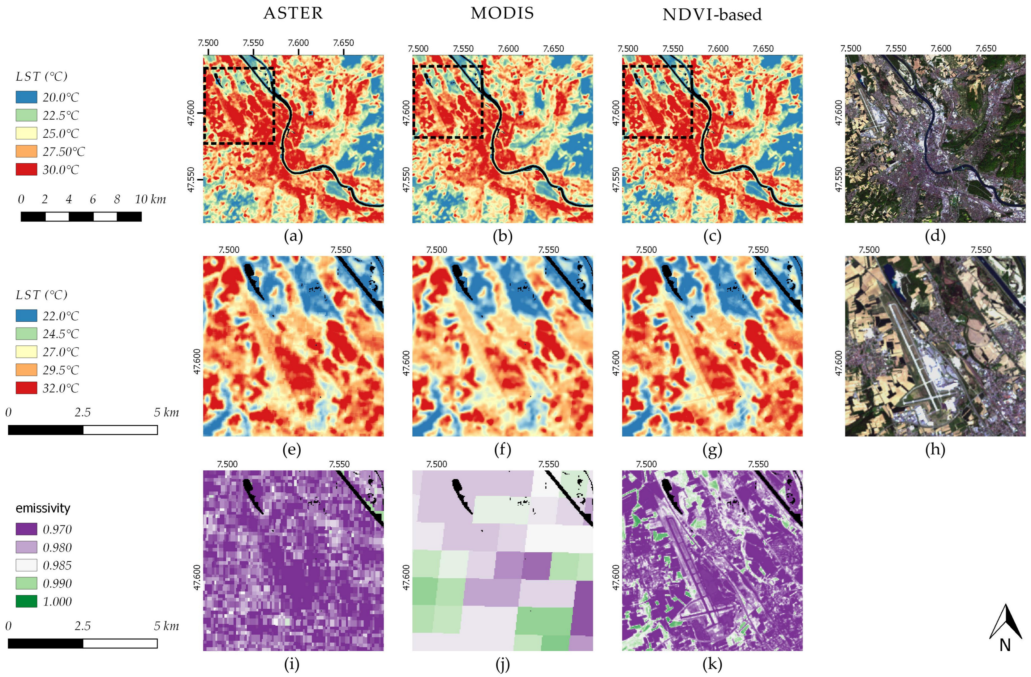
Figure 4a–c shows the Landsat 8 LST maps for the area of Basel, Switzerland on the 24 April 2015, using ASTER- (Figure 4a), MODIS- (Figure 4b) and NDVI-based (Figure 4c) emissivity products. Figure 4d is the Landsat 8 RGB (red green blue) image from the same date. Figure 4e–h presents a zoom in the outlined area of the Basel airport (EuroAirport Basel Mulhouse Freiburg) and Figure 4i–k presents the corresponding emissivity.
The LST maps using different emissivity sources in Figure 4a–c show similar results, as expected from the earlier discussion (see Figure 3b). A closer look at the zoomed area reveals some of the strengths and weaknesses of each different emissivity-derived LST. At the bottom half of the images in the first row, the LST with NDVI-based emissivity (Figure 4c) outlined better the vegetated areas than the LST with ASTER and MODIS emissivity. The NDVI-based emissivity captures well the emissivity of vegetation, which is in the peak in this image since it was acquired during April. This is even more evident in the second row, zoomed-in area in Figure 4. Another noticeable difference in the LST refers to the area of the airport. The ASTER emissivity seems to provide better estimates for the airport area, which is expected to be hotter than the surrounding area. In the third row of Figure 4, the NDVI-based emissivity seems to capture better than ASTER and MODIS the spatial variability of emissivity. The ASTER emissivity product is assumed to be more accurate in the case of non-vegetated surfaces, since it is derived from a combination of long-term emissivity data, while the NDVI-based emissivity assumes a constant emissivity value for non-vegetated surfaces.
3.1.3. Overall Accuracy Assessment of the Landsat LST Products
Following the process of comparison that was described in Section 2.4, the average RMSE for all 147 comparisons was initially computed at 1.89 °C. This can be improved by taking advantage of the findings described in Section 3.1.1, using only the SAFREE database when estimating LST from Landsat 5 and the TIGR2 for Landsat 7. Another improvement can be made by choosing the best emissivity source based on the area as described in Section 3.1.2. Therefore, considering all these adjustments, the final RMSE was found to be 1.40 °C (bias −0.31) for Landsat 5, 1.71 °C (bias 0.77) for Landsat 7, 1.31 °C (bias 0.1) for Landsat 8. Furthermore, an overall RMSE of 1.52 °C was estimated for all Landsat sensors used in this study.
3.2. Landsat LST Web Application
The LST products for Landsat 5, 7 and 8 at 30 m spatial resolution are publicly available through a web application that was developed for this purpose and it is accessible at: http://rslab.gr/downloads_LandsatLST.html. This web application automatically updates with the latest available satellite data, since it is linked to the GEE catalogue, which is updated frequently. The availability of data depends on the operational period of the respective satellites. The Landsat 5 archive extends from March 1984 to May 2012, the Landsat 7 archive extends from May 1999 to present and the Landsat 8 archive from April 2013 to present. LST products can be created for each Landsat sensor for the time period of its operation, shown in Table 1, using NDVI-based emissivity. Although products are available for the same periods using ASTER emissivity, their use is suggested based on the guidelines we provide below. Landsat LST products with the use of MODIS emissivity are available for the period 2002 up to present.
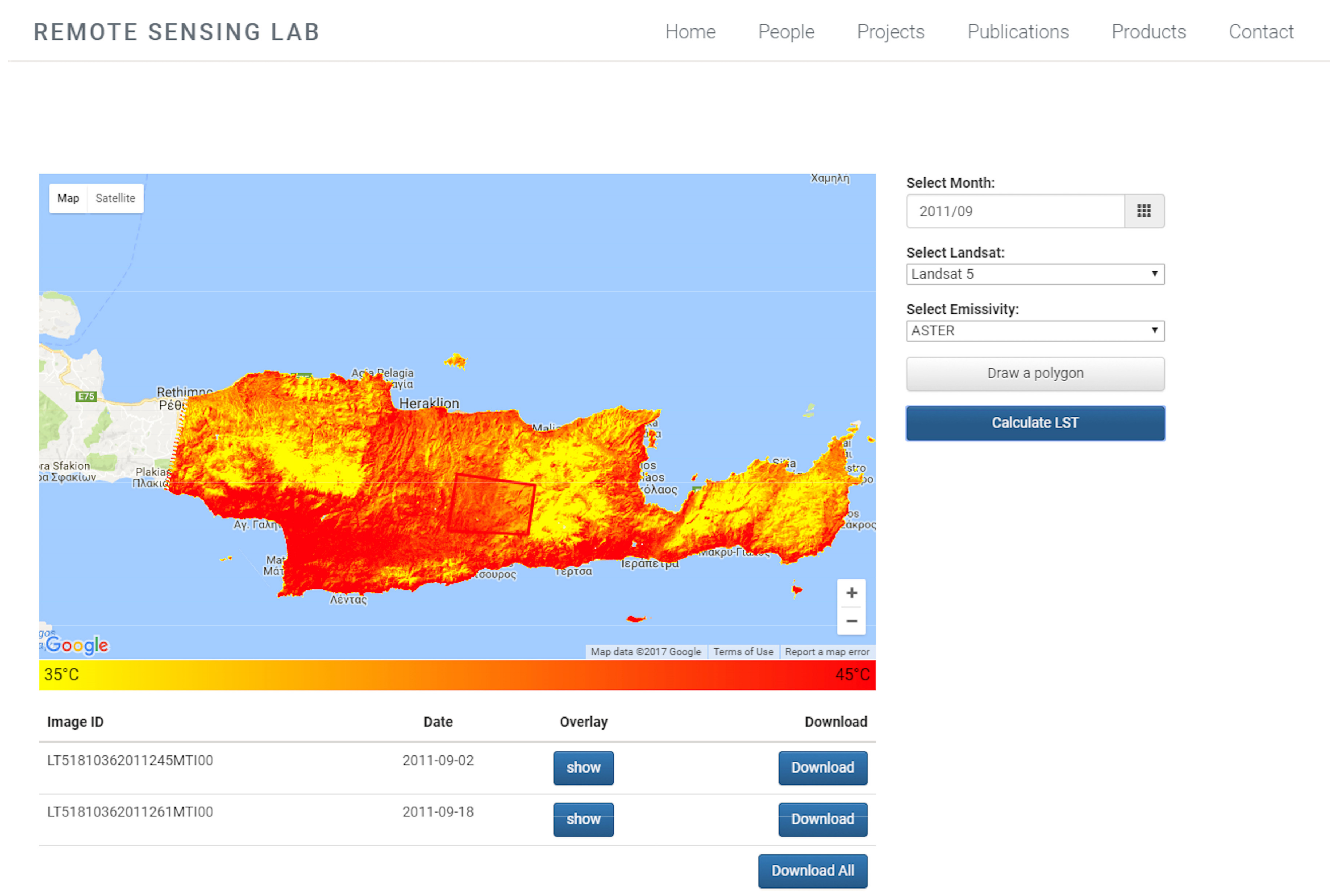
Figure 5 shows a screenshot of the web application. The user can choose the desired date range, Landsat satellite and emissivity source; and draw a polygon to identify an area of interest. Then, by clicking the “Calculate LST” button, the calculations are performed based on the user preferences. The LST products are presented in the form of a map layer overlaid to Google Maps. The LST product(s) corresponding to the date range and area of interest are listed under the map and they are available for download either individually, or as a batch file. Due to the computational limitations, a maximum date range of one month is allowed in the current release of the web application. This will be improved in future releases to allow larger datasets to be handled at once.
Using the ASTER emissivity is recommended for cases of natural/isolated landscapes, with not-significant land cover changes, as was indicated by our analysis; or to use it for LST retrievals from Landsat observations acquired between 2000 and 2008, which is the time period that corresponds to the data acquisition of this ASTER product. The NDVI-based emissivity should be used in cases of intense phenological changes in vegetated areas. The MODIS emissivity should be used in cases of areas with extended homogeneous areas that are changing over time, i.e., extended deciduous forests.
The application was built with the use of HTML (hypertext markup Llanguage), JavaScript, CSS (cascading style sheets), JQUERY for the front end and GEE’s Python API for the back end, as explained in Section 2.3. It provides instant access to global, up-to-date, LST data and it is light-weight in terms of computations. This is achieved with the use of GEE, which enables instant access to the large satellite data archive and transfers all the computational and storage needs to Google’s infrastructure. Moreover, the user does not need to install any software or download any data for processing, as opposed to currently available applications [22,24]. The Landsat LST web application can even run from mobile devices with limited power for a quick snapshot of the LST of an area.
Other sources of data, capable of improving the accuracy of our LST estimations, such as temperature and emissivity retrievals from geostationary platforms like MSG (Meteosat Second Generation) [52], will also be taken into account in our analysis, as soon as they are available in GEE. Feedback by the scientific community on the quality of our LST products is highly welcome and we encourage users that own in-situ observations to publish validation studies.
4. Conclusions
LST information from Landsat is not easily calculated, and so far, it is not directly provided as a standard product. Many studies propose methods and algorithms for retrieving LST from Landsat observations, but only experts can easily implement these approaches. Landsat image downloading and ancillary atmospheric data is also needed and the installation of extra tools and software is required in most cases. This study presents an online application for LST estimation from Landsat 5, 7 and 8 that requires the least possible time and effort to provide maps on-the-fly and without the need for extra resources from the user. For global coverage and the whole Landsat archive, this is only possible using advanced cloud computing technologies, i.e., the GEE. The GEE data catalogue includes all the Landsat imagery and it transfers all the heavy computational processes to cloud computing servers. The user only needs to define the time range and area of interest and receives the Landsat LST maps and products in seconds.
The LST estimation method implements a SC algorithm because it allows LST retrieval with the use of one thermal channel. This allowed for algorithm consistency between Landsat 5, 7 and 8. Since for SC algorithms the emissivity is provided from external sources, the developed web application provides the flexibility to choose between three different emissivity sources: ASTER, MODIS and NDVI-based. An accuracy analysis using ASTER and LST estimations from Landsat using alternative approaches as reference datasets, indicated that the LST can be retrieved from Landsat 5, 7 and 8 within an overall accuracy of 1.52 °C (RMSE). The three different emissivity sources did not significantly differentiate LST estimations; however, recommendations on emissivity source selection were made in this study: the analysis revealed that ASTER-derived emissivity performs better for areas with no significant land cover changes; the NDVI-based emissivity captures phenological changes and their spatial pattern well; and the MODIS-derived emissivity is suitable for extended homogeneous areas.
Further improvement of the web application includes adding extra options for users such as a minimum, maximum and average extractor for every image, increasing the maximum date range, as well as further investigation of the results in order to improve the accuracy of the LST products for specific areas at local scales. There is room for improvement in the calculation of the NDVI-based emissivity, which can provide more accurate estimations with varying definitions of NDVInonveg and NDVIveg in Equation (6), such as the NDVI-THM (NDVI threshold method) approach [53]. Improved emissivity retrieval methods for urban environments [41] are considered for future implementation, to ensure accurate estimation of energy budget components at local scale. The possibility of a consolidated emissivity product is also under consideration. The usability of applications like the one developed in this study are not yet mainstream. Therefore, we appreciate also any feedback by users of the web application, based on their specific needs, in order to improve it and to provide tailored solutions to users in future releases.
Acknowledgments
The project leading to this application has received partial funding from the European Union’s Horizon 2020 research and innovation program under grant agreement No. 637519 (URBANFLUXES). Work by M.A. was done at the Jet Propulsion Laboratory/California Institute of Technology under contract with the National Aeronautics and Space Administration. We also want to thank Mattia Marconcini from DLR (German Aerospace Agency) for providing the alternative Landsat LST products using ATCOR, that we used for assessing the accuracy of Landsat 5 and 8 LST products. Finally, we would like to thank all the people in the GEE developer forum and particularly Noel Gorelick for their assistance regarding technical support for GEE.
Author Contributions
D.P. wrote the paper, conceived and performed the comparison experiments, analysed the results as well as designed and created the application. Z.M. overviewed the whole process, reviewed the paper, provided comments, provided the MATLAB code that was used for comparing our LST products with the reference data and assisted in the interpretation of the results. N.C. overviewed the whole process, reviewed the paper, provided comments and assisted in the interpretation of the comparison results. M.A. provided the ASTER LST products used as a reference for assessing the accuracy of the Landsat 7 LST products, reviewed the paper and provided comments.
Conflicts of Interest
The authors declare no conflict of interest.
References
- Quattrochi, D.A.; Luvall, J.C. Thermal infrared remote sensing for analysis of landscape ecological processes: Methods and applications. Landsc. Ecol. 1999, 14, 577–598. [Google Scholar] [CrossRef]
- Chrysoulakis, N.; Lopes, M.; San José, R.; Grimmond, C.S.B.; Jones, M.B.; Magliulo, V.; Klostermann, J.E.M.; Synnefa, A.; Mitraka, Z.; Castro, E.A.; et al. Sustainable urban metabolism as a link between bio-physical sciences and urban planning: The BRIDGE project. Landsc. Urban Plan. 2013, 112, 100–117. [Google Scholar] [CrossRef]
- Chrysoulakis, N.; Marconcini, M.; Gastellu-Etchegorry, J.P.; Grimmond, C.S.B.; Feigenwinter, C.; Lindberg, F.; Del Frate, F.; Klostermann, J.; Mitraka, Z.; Esch, T.; et al. Anthropogenic Heat Flux Estimation from Space: Results of the second phase of the URBANFLUXES Project. In Proceeding of the Joint Urban Remote Sensing Event (JURSE 2017), Dubai, UAE, 30 March–1 April 2017. [Google Scholar]
- Kustas, W.; Anderson, M. Advances in thermal infrared remote sensing for land surface modeling. Agric. For. Meteorol. 2009, 149, 2071–2081. [Google Scholar] [CrossRef]
- Karnieli, A.; Agam, N.; Pinker, R.T.; Anderson, M.; Imhoff, M.L.; Gutman, G.G.; Panov, N.; Goldberg, A. Use of NDVI and land surface temperature for drought assessment: Merits and limitations. J. Clim. 2010, 23, 618–633. [Google Scholar] [CrossRef]
- Anderson, M.C.; Norman, J.M.; Kustas, W.P.; Houborg, R.; Starks, P.J.; Agam, N. A thermal-based remote sensing technique for routine mapping of land-surface carbon, water and energy fluxes from field to regional scales. Remote Sens. Environ. 2008, 112, 4227–4241. [Google Scholar] [CrossRef]
- Zhang, R.; Tian, J.; Su, H.; Sun, X.; Chen, S.; Xia, J. Two improvements of an operational two-layer model for terrestrial surface heat flux retrieval. Sensors 2008, 8, 6165–6187. [Google Scholar] [CrossRef] [PubMed]
- Hansen, J.; Ruedy, R.; Sato, M.; Lo, K. Global surface temperature change. Rev. Geophys. 2010, 48, RG4004. [Google Scholar] [CrossRef]
- Masiello, G.; Serio, C.; Venafra, S.; Liuzzi, G.; Göttsche, F.; Trigo, I.F.; Watts, P. Kalman filter physical retrieval of surface emissivity and temperature from SEVIRI infrared channels: A validation and intercomparison study. Atmos. Meas. Tech. 2015, 8, 2981–2997. [Google Scholar] [CrossRef]
- Ottlé, C.; Vidal-Madjar, D. Estimation of land surface temperature with NOAA9 data. Remote Sens. Environ. 1992, 40, 27–41. [Google Scholar] [CrossRef]
- Benas, N.; Chrysoulakis, N.; Cartalis, C. Trends of urban surface temperature and heat island characteristics in the Mediterranean. Theor. Appl. Climatol. 2016, 1–10. [Google Scholar] [CrossRef]
- Weng, Q.; Lu, D.; Schubring, J. Estimation of land surface temperature-vegetation abundance relationship for urban heat island studies. Remote Sens. Environ. 2004, 89, 467–483. [Google Scholar] [CrossRef]
- Tomlinson, C.J.; Chapman, L.; Thornes, J.E.; Baker, C. Remote sensing land surface temperature for meteorology and climatology: A review. Meteorol. Appl. 2011, 18, 296–306. [Google Scholar] [CrossRef]
- Rogan, J.; Ziemer, M.; Martin, D.; Ratick, S.; Cuba, N.; DeLauer, V. The impact of tree cover loss on land surface temperature: A case study of central Massachusetts using Landsat Thematic Mapper thermal data. Appl. Geogr. 2013, 45, 49–57. [Google Scholar] [CrossRef]
- Van Leeuwen, T.T.; Frank, A.J.; Jin, Y.; Smyth, P.; Goulden, M.L.; van der Werf, G.R.; Randerson, J.T. Optimal use of land surface temperature data to detect changes in tropical forest cover. J. Geophys. Res. 2011, 116, 1–16. [Google Scholar] [CrossRef]
- Ayanlade, A. Remote sensing approaches for land use and land surface temperature assessment: A review of methods. Int. J. Image Data Fusion 2017, 8, 188–201. [Google Scholar] [CrossRef]
- Wan, Z. A generalized split-window algorithm for retrieving land-surface temperature from space. IEEE Trans. Geosci. Remote Sens. 1996, 34, 892–905. [Google Scholar] [CrossRef]
- Coll, C.; Caselles, V. A split-window algorithm for land surface temperature from advanced very high resolution radiometer data: Validation and algorithm comparison. J. Geophys. Res. 1997, 102, 16697–16713. [Google Scholar] [CrossRef]
- Jimenez-Munoz, J.C.; Cristobal, J.; Sobrino, J.A.; Sòria, G.; Ninyerola, M.; Pons, X. Revision of the single-channel algorithm for land surface temperature retrieval from Landsat thermal-infrared data. IEEE Trans. Geosci. Remote Sens. 2009, 47, 339–349. [Google Scholar] [CrossRef]
- Jimenez-Munoz, J.C.; Sobrino, J.A.; Skokovic, D.; Mattar, C.; Cristobal, J. Land surface temperature retrieval methods from Landsat-8 thermal infrared sensor data. IEEE Geosci. Remote Sens. Lett. 2014, 11, 1840–1843. [Google Scholar] [CrossRef]
- Quantum Geographic Information System (QGIS). Available online: http://www.qgis.org/en/site/index.html (accessed on 30 August 2017).
- Ndossi, M.I.; Avdan, U. Application of open source coding technologies in the production of Land Surface Temperature (LST) maps from Landsat: A PyQGIS plugin. Remote Sens. 2016, 8, 413. [Google Scholar] [CrossRef]
- ERDAS Field Guide Manual. Available online: http://gisknowledge.net/topic/imagine_training/imagine_field_guide_05.pdf (accessed on 19 September 2017).
- Avdan, U.; Jovanovska, G. Algorithm for automated mapping of land surface temperature using Landsat 8 satellite data. J. Sens. 2016, 2016, 1–8. [Google Scholar] [CrossRef]
- Landsat Higher Level Science Data Products. Available online: https://landsat.usgs.gov/landsat-higher-level-science-data-products (accessed on 6 September 2017).
- Yu, X.; Guo, X.; Wu, Z. Land surface temperature retrieval from Landsat 8 TIRS-comparison between radiative transfer equation-based method, split window algorithm and single channel method. Remote Sens. 2014, 6, 9829–9852. [Google Scholar] [CrossRef]
- NASA EOSDIS Land Processes DAAC (LPDAAC). ASTER Global Emissivity Dataset, 100-Meter, HDF5. 2014. Available online: https://data.nasa.gov/Earth-Science/ASTER-Global-Emissivity-Database-100-meter-HDF5-V0/mijt-xkx7 (accessed on 20 November 2017).
- Hulley, G.C.; Hook, S.J.; Abbott, E.; Malakar, N.; Islam, T.; Abrams, M. The ASTER Global Emissivity Dataset (ASTER GED): Mapping Earth’s emissivity at 100 meter spatial scale. Geophys. Res. Lett. 2015, 42, 7966–7976. [Google Scholar] [CrossRef]
- Wan, Z.; Hook, S.; Hulley, G. MOD11A1 MODIS/Terra Land Surface Temperature/Emissivity Daily L3 Global 1 km SIN Grid V006. 2015. Available online: https://lpdaac.usgs.gov/dataset_discovery/modis/modis_products_table/mod11a1_v006 (accessed on 20 November 2017).
- Carlson, T.N.; Ripley, D.A. On the relation between NDVI, fractional vegetation cover, and leaf area index. Remote Sens. Environ. 1997, 62, 241–252. [Google Scholar] [CrossRef]
- Gorelick, N.; Hancher, M.; Dixon, M.; Ilyushchenko, S.; Thau, D.; Moore, R. Google Earth Engine: Planetary-scale geospatial analysis for everyone. Remote Sens. Environ. 2017. [Google Scholar] [CrossRef]
- Sobrino, J.A.; Jiménez-Muñoz, J.C.; Paolini, L. Land surface temperature retrieval from Landsat TM 5. Remote Sens. Environ. 2004, 90, 434–440. [Google Scholar] [CrossRef]
- Dash, P.; Göttsche, F.-M.; Olesen, F.-S.; Fischer, H. Land surface temperature and emissivity estimation from passive sensor data: Theory and practice-current trends. Int. J. Remote Sens. 2002, 23, 2563–2594. [Google Scholar] [CrossRef]
- What Are Band Designations Landsat Satellites. Available online: https://landsat.usgs.gov/what-are-band-designations-landsat-satellites (accessed on 1 September 2017).
- Landsat 8 OLI and TIRS. Available online: https://lta.cr.usgs.gov/L8 (accessed on 4 September 2017).
- 2010_Landsat_Updates. Available online: https://landsat.usgs.gov/sites/default/files/documents/2010_Landsat_Updates.pdf (accessed on 4 September 2017).
- Gao, B.-C.; Kaufman, Y.J. Water vapor retrievals using Moderate Resolution Imaging Spectroradiometer (MODIS) near-infrared channels. J. Geophys. Res. Atmos. 2003, 108. [Google Scholar] [CrossRef]
- Zhu, Z.; Woodcock, C.E. Object-based cloud and cloud shadow detection in Landsat imagery. Remote Sens. Environ. 2012, 118, 83–94. [Google Scholar] [CrossRef]
- Zhu, Z.; Wang, S.; Woodcock, C.E. Improvement and expansion of the Fmask algorithm: Cloud, cloud shadow, and snow detection for Landsats 4–7, 8, and Sentinel 2 images. Remote Sens. Environ. 2015, 159, 269–277. [Google Scholar] [CrossRef]
- Masek, J.G.; Vermote, E.F.; Saleous, N.; Wolfe, R.; Hall, F.G.; Huemmrich, F.; Gao, F.; Kutler, J.; Lim, T.K. LEDAPS Landsat Calibration, Reflectance, Atmospheric Correction Preprocessing Code. 2012. Available online: https://daac.ornl.gov/MODELS/guides/LEDAPS.html (accessed on 20 November 2017).
- Mitraka, Z.; Chrysoulakis, N.; Kamarianakis, Y.; Partsinevelos, P.; Tsouchlaraki, A. Improving the estimation of urban surface emissivity based on sub-pixel classification of high resolution satellite imagery. Remote Sens. Environ. 2012, 117, 125–134. [Google Scholar] [CrossRef]
- Chen, F.; Yang, S.; Su, Z.; Wang, K. Effect of emissivity uncertainty on surface temperature retrieval over urban areas: Investigations based on spectral libraries. ISPRS J. Photogramm. Remote Sens. 2016, 114, 53–65. [Google Scholar] [CrossRef]
- Snyder, W.C.; Wan, Z. BRDF models to predict spectral reflectance and emissivity in the thermal infrared. IEEE Trans. Geosci. Remote Sens. 1998, 36, 214–225. [Google Scholar] [CrossRef]
- Wan, Z. MODIS Land-Surface Temperature Algorithm Theoretical Basis Document (LST ATBD), Version 3.3. Available online: https://modis.gsfc.nasa.gov/data/atbd/atbd_mod11.pdf (accessed on 6 September 2017).
- Kalnay, E.; Kanamitsu, M.; Kistler, R.; Collins, W.; Deaven, D.; Gandin, L.; Iredell, M.; Saha, S.; White, G.; Woollen, J.; et al. The NCEP/NCAR 40-year reanalysis project. Bull. Am. Meteorol. Soc. 1996, 77, 437–471. [Google Scholar] [CrossRef]
- Chrysoulakis, N.; Kamarianakis, Y.; Xu, L.; Mitraka, Z.; Ding, J. Combined use of MODIS, AVHRR and radiosonde data for the estimation of spatiotemporal distribution of precipitable water. J. Geophys. Res. Atmos. 2008, 113. [Google Scholar] [CrossRef]
- Dee, D.P.; Uppala, S.M.; Simmons, A.J.; Berrisford, P.; Poli, P.; Kobayashi, S.; Andrae, U.; Balmaseda, M. A.; Balsamo, G.; Bauer, P.; et al. The ERA-Interim reanalysis: Configuration and performance of the data assimilation system. Q. J. R. Meteorol. Soc. 2011, 137, 553–597. [Google Scholar] [CrossRef]
- Gillespie, A.; Rokugawa, S.; Matsunaga, T.; Cothern, J.S.; Hook, S.; Kahle, A.B. A temperature and emissivity separation algorithm for Advanced Spaceborne Thermal Emission and Reflection Radiometer (ASTER) images. IEEE Trans. Geosci. Remote Sens. 1998, 36, 1113–1126. [Google Scholar] [CrossRef]
- Hulley, G.C.; Hughes, C.G.; Hook, S.J. Quantifying uncertainties in land surface temperature and emissivity retrievals from ASTER and MODIS thermal infrared data. J. Geophys. Res. 2012, 117. [Google Scholar] [CrossRef]
- Hook, S.J.; Vaughan, R.G.; Tonooka, H.; Schladow, S.G. Absolute Radiometric in-Flight Validation of Mid Infrared and Thermal Infrared Data from ASTER and MODIS on the Terra Spacecraft Using the Lake Tahoe, CA/NV, USA, Automated Validation Site. IEEE Trans. Geosci. Remote Sens. 2007, 45, 1798–1807. [Google Scholar] [CrossRef]
- Richter, R.; Schläpfer, D. Atmospheric/Topographic Correction for Satellite Imagery (ATCOR-2/3 User Guide ATCOR-2/3 User Guide Version 9.0.2, March 2016). Available online: http://www.rese.ch/pdf/atcor3_manual.pdf (accessed on 21 November 2017).
- Blasi, M.G.; Liuzzi, G.; Masiello, G.; Serio, C.; Telesca, V.; Venafra, S. Surface parameters from SEVIRI observations through a kalman filter approach: Application and evaluation of the scheme to the southern Italy. Tethys 2016, 2016, 1–19. [Google Scholar] [CrossRef]
- Sobrino, J.A.; Jiménez-Muñoz, J.C.; Sòria, G.; Romaguera, M.; Guanter, L.; Moreno, J.; Plaza, A.; Martínez, P. Land surface emissivity retrieval from different VNIR and TIR sensors. IEEE Trans. Geosci. Remote Sens. 2008, 46, 316–327. [Google Scholar] [CrossRef]
Figure 1.
LST estimation algorithm in the application. The user sets his preferences for the geographical area, the date range, the source of emissivity and the preferred Landsat in the front end. In the back end a function joins the GEE image collections of Landsat and emissivity data, whereas a second function adds the PW (precipitable water) information. The joined collection is then used for the LST estimation. The process is the same in GEE ‘playground’ as well as in the web application.

Figure 2.
LST RMSE (root mean square error) boxplots for each coefficient table, where × is the average, and the horizontal line inside box is the median. (a) Landsat 5 RMSE boxplots for each coefficient table calculated from all three available Landsat 5 delivered reference data; (b) Landsat 7 RMSE boxplots for each coefficient table calculated from all six ASTER reference images.
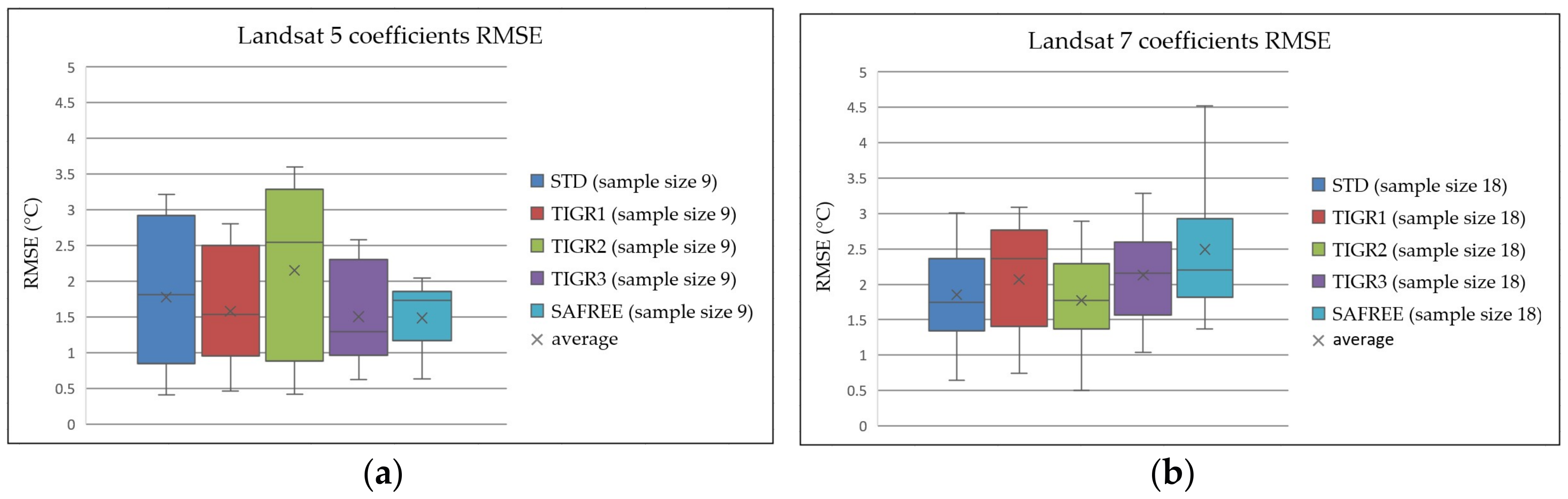
Figure 3.
Boxplots of LST RMSE results based on the source of emissivity (ASTER, MODIS, NDVI) for natural/isolated landscapes and urban/peri-urban areas, and the horizontal line inside each box is the median. (a) Natural/isolated landscapes category contains the RMSE boxplots from the Amazon forest, the West Virginia Mountains and Sahara Desert; (b) Urban/peri-urban areas category contains the RMSE boxplots from Bangkok, Dubai, Tokyo and all Heraklion and Basel images.
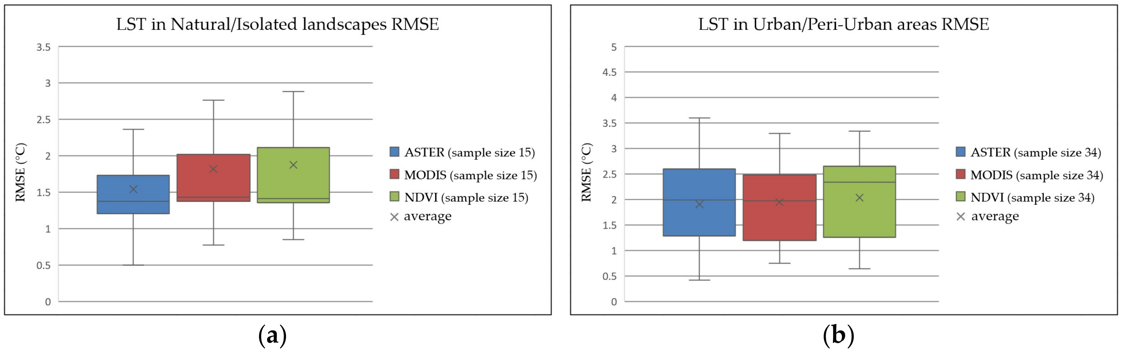
Figure 4.
Landsat LST estimations with different emissivity sources in the area of Basel, Switzerland, 24 April 2015: (a) LST estimated with ASTER emissivity product; (b) LST estimated with MODIS emissivity; (c) LST estimated with NDVI-based emissivity; (d) true-color composition of the Landsat 8 image of 24 April 2015; (e) LST in the Basel airport area using ASTER emissivity; (f) LST in the Basel airport area using MODIS emissivity; (g) LST in the Basel airport area using NDVI-based emissivity; (h) true-color composition of the Landsat 8 image of 24 April 2015 in the Basel airport area (i) ASTER emissivity product in the Basel airport; (j) MODIS emissivity product in the Basel airport; (k) NDVI-based emissivity in the Basel airport. Black color in all cases represents masked areas.

Figure 5.
Screenshot of the Landsat LST web application. The users set their preferences for the date range, preferred Landsat and emissivity source on the right-hand side. The option ‘Draw a polygon’ allows the user to draw the area of interest on the map. An example is shown here for the area of Heraklion, Greece. Landsat 5 scenes that correspond to this specific request, their IDs and acquisition date are shown in a table at the bottom, along with the respective visualization and download options. In this screenshot, the LST product corresponding to the first image in said table is shown overlaid on Google Maps. The missing values correspond to clouds, cloud shadows and water surfaces.


Table 1.
Landsat 5, 7 and 8 thermal bands: wavelengths, spatial resolution and time period covered.
| Thermal Band(s) # | Wavelength (μm) | Spatial Resolution (m) | Time Period | |
|---|---|---|---|---|
| Landsat 5 | Band 6 | 10.40–12.50 | 120 (30) 1 | March 1984–May 2012 |
| Landsat 7 | Band 6 | 10.40–12.50 | 60 (30) 1 | April 1999–Present |
| Landsat 8 | Band 10 Band 11 | 10.60–11.19 11.50–12.51 | 100 (30) 1 | April 2013–Present |
Table 2.
List of products in the GEE catalogue used to estimate the Landsat LST.
| Data | GEE Product Identifier |
|---|---|
| Landsat 5, Radiance at sensor from band 6 | LANDSAT/LT5_L1T |
| Landsat 5, Brightness temperature from band 6 | LANDSAT/LT5_L1T_TOA_FMASK |
| Landsat 7, Radiance at sensor from band 6 | LANDSAT/LE7_L1T |
| Landsat 7, Brightness temperature from band 6 | LANDSAT/LE7_L1T_TOA_FMASK |
| Landsat 8, Radiance at sensor from band 10 | LANDSAT/LC8_L1T |
| Landsat 8, Brightness temperature from band 10 | LANDSAT/LC8_L1T_TOA_FMASK |
| MODIS Daily average emissivity from bands 31 and 32 | MODIS/MOD11A1 |
| NCEP/NCAR 6-hour temporal resolution of the total column water vapour from a single band | NCEP_RE/surface_wv |
| ASTER 1 Global image with emissivity from 2000–2008 clear-sky pixels from band 14 | NASA/ASTER_GED/AG100_003 |
| Landsat 5, Surface Reflectance product | LANDSAT/LT5_SR |
| Landsat 7, Surface Reflectance product | LEDAPS/LE7_L1T_SR |
| Landsat 8, Surface Reflectance Product | LANDSAT/LC8_SR |
| Fmask, from extra band in GEE’s Brightness temperature products | LANDSAT/LT5_L1T_TOA_FMASK LANDSAT/LE7_L1T_TOA_FMASK LANDSAT/LC8_L1T_TOA_FMASK |
Table 3.
Emissivity sources presented with their corresponding band number, band wavelength and temporal resolution.
Table 3.
Emissivity sources presented with their corresponding band number, band wavelength and temporal resolution.
| Emissivity Source | Band(s) # | Wavelength (μm) | Temporal Resolution | Spatial Resolution (m) |
|---|---|---|---|---|
| ASTER | 10 11 12 13 14 | 8.125–8.825 8.475–8.825 8.925–9.275 10.25–10.95 10.95–11.65 | 1 static image with average pixel values from 2000–2008 | 90 |
| MODIS | 31 32 | 10.78–11.28 11.77–12.27 | Daily, 2000–present | 1000 |
| NDVI based Landsat 5 | 3 1 4 1 | 0.63–0.69 0.76–0.90 | About every 16 days, 1984–2012 | 30 |
| NDVI based Landsat 7 | 3 1 4 1 | 0.63–0.69 0.77–0.90 | About every 16 days, 1999–present | 30 |
| NDVI based Landsat 8 | 4 1 5 1 | 0.636–0.673 0.851–0.879 | About every 16 days, 2013–2017 | 30 |
1 These are the red and near-infrared bands from which the NDVI is calculated and then the NDVI-based emissivity. Not to be confused with the MODIS (Moderate Resolution Imaging Spectroradiometer) and ASTER (Advanced Spaceborne Thermal Emission and Reflection Radiometer) bands in this table, which directly provide the emissivity values.
Table 4.
List of reference images used for accuracy assessment, the area they cover, the date of acquisition, the spatial resolution, satellite source of acquisition and the PW content.
Table 4.
List of reference images used for accuracy assessment, the area they cover, the date of acquisition, the spatial resolution, satellite source of acquisition and the PW content.
| Area of the Scene | Satellite | Acquisition Date | Spatial Resolution (m) | Location (Latitude, Longitude) | Area Size (km2) | PW (g/cm2) |
|---|---|---|---|---|---|---|
| The West Virginia mountains | ASTER | 11 October 2004 | 90 | 38.6621, −80.4140 | 2.449 | 0.72 |
| Amazon forest | ASTER | 7 September 2010 | 90 | −0.2032, −57.4076 | 2.321 | 4.32 |
| Bangkok | ASTER | 11 December 2014 | 90 | 13.8167, 100.4589 | 2.660 | 2.42 |
| Sahara Desert | ASTER | 27 October 2016 | 90 | 26.2330, 26.2820 | 2.346 | 2.20 |
| Dubai | ASTER | 29 June 2009 | 90 | 25.2831, 55.3724 | 1.560 | 0.83 |
| Tokyo | ASTER | 10 May 2015 | 90 | 35.6729, 139.7488 | 2.522 | 1.10 |
| Basel | Landsat 5 | 31 July 2010 | 30 | 47.5608, 7.5846 | 415 | 1.54 |
| Basel | Landsat 8 | 24 April 2015 | 30 | 47.5608, 7.5846 | 415 | 0.97 |
| Basel | Landsat 8 | 23 August 2016 | 30 | 47.5608, 7.5846 | 415 | 2.92 |
| Heraklion | Landsat 5 | 19 February 2010 | 30 | 35.3398, 25.1330 | 191 | 1.06 |
| Heraklion | Landsat 5 | 16 July 2011 | 30 | 35.3398, 25.1330 | 191 | 2.02 |
| Heraklion | Landsat 8 | 29 July 2016 | 30 | 35.3398, 25.1330 | 191 | 2.60 |
| Heraklion | Landsat 8 | 7 March 2016 | 30 | 35.3398, 25.1330 | 191 | 1.36 |
© 2017 by the authors. Licensee MDPI, Basel, Switzerland. This article is an open access article distributed under the terms and conditions of the Creative Commons Attribution (CC BY) license (http://creativecommons.org/licenses/by/4.0/).
Share and Cite
MDPI and ACS Style
Parastatidis, D.; Mitraka, Z.; Chrysoulakis, N.; Abrams, M. Online Global Land Surface Temperature Estimation from Landsat. Remote Sens. 2017, 9, 1208. https://doi.org/10.3390/rs9121208
AMA Style
Parastatidis D, Mitraka Z, Chrysoulakis N, Abrams M. Online Global Land Surface Temperature Estimation from Landsat. Remote Sensing. 2017; 9(12):1208. https://doi.org/10.3390/rs9121208
Chicago/Turabian StyleParastatidis, David, Zina Mitraka, Nektrarios Chrysoulakis, and Michael Abrams. 2017. "Online Global Land Surface Temperature Estimation from Landsat" Remote Sensing 9, no. 12: 1208. https://doi.org/10.3390/rs9121208
Note that from the first issue of 2016, this journal uses article numbers instead of page numbers. See further details here.