Article

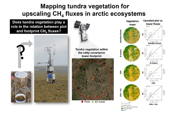
Upscaling CH4 Fluxes Using High-Resolution Imagery in Arctic Tundra Ecosystems

by
Scott J. Davidson
1,2,*,
Maria J. Santos
3,
Victoria L. Sloan
2,
Kassandra Reuss-Schmidt
1,
Gareth K. Phoenix
1,
Walter C. Oechel
2,4 and
Donatella Zona
1,2
1
Department of Animal and Plant Sciences, University of Sheffield, Western Bank, Sheffield S10 2TN, UK
2
Department of Biology, San Diego State University, 5500 Campanile Drive, San Diego, CA 92182, USA
3
Department of Innovation, Environmental and Energy Sciences, Utrecht University, 3512 JE Utrecht, The Netherlands
4
College of Environmental Sciences, University of Exeter, Exeter EX4 4RU, UK
*
Author to whom correspondence should be addressed.
Remote Sens. 2017, 9(12), 1227; https://doi.org/10.3390/rs9121227
Submission received: 25 October 2017 / Revised: 23 November 2017 / Accepted: 27 November 2017 / Published: 28 November 2017
(This article belongs to the Special Issue Remote Sensing of Arctic Tundra)

Abstract

:
Arctic tundra ecosystems are a major source of methane (CH4), the variability of which is affected by local environmental and climatic factors, such as water table depth, microtopography, and the spatial heterogeneity of the vegetation communities present. There is a disconnect between the measurement scales for CH4 fluxes, which can be measured with chambers at one-meter resolution and eddy covariance towers at 100–1000 m, whereas model estimates are typically made at the ~100 km scale. Therefore, it is critical to upscale site level measurements to the larger scale for model comparison. As vegetation has a critical role in explaining the variability of CH4 fluxes across the tundra landscape, we tested whether remotely-sensed maps of vegetation could be used to upscale fluxes to larger scales. The objectives of this study are to compare four different methods for mapping and two methods for upscaling plot-level CH4 emissions to the measurements from EC towers. We show that linear discriminant analysis (LDA) provides the most accurate representation of the tundra vegetation within the EC tower footprints (classification accuracies of between 65% and 88%). The upscaled CH4 emissions using the areal fraction of the vegetation communities showed a positive correlation (between 0.57 and 0.81) with EC tower measurements, irrespective of the mapping method. The area-weighted footprint model outperformed the simple area-weighted method, achieving a correlation of 0.88 when using the vegetation map produced with the LDA classifier. These results suggest that the high spatial heterogeneity of the tundra vegetation has a strong impact on the flux, and variation indicates the potential impact of environmental or climatic parameters on the fluxes. Nonetheless, assimilating remotely-sensed vegetation maps of tundra in a footprint model was successful in upscaling fluxes across scales.

Graphical Abstract

1. Introduction

Arctic tundra ecosystems emit substantial amounts of methane (CH4), which is of critical importance given the rate of climate change occurring at northern latitudes. The arctic is currently warming at nearly double the global average [1], and this increase in temperature may magnify CH4 emissions. Nearly 8–30 Tg y−1 of CH4 is emitted from natural arctic wetland ecosystems to the atmosphere [2,3], which corresponds to about 10% of the total CH4 emitted by natural wetland ecosystems globally (100–200 Tg y−1) [4,5]. Furthermore, due to CH4 global warming potential [1,6], an increase in emissions could result in additional atmospheric warming [7,8]. Current and future arctic CH4 emissions are affected by spatially heterogeneous vegetation communities, environmental and climatic parameters and microtopographic characteristics [9,10,11]. Different vegetation communities emit CH4 at different rates [12], therefore, plant community distributions could be used to upscale CH4 fluxes to the landscape scale and improve emission estimates in carbon cycle [13,14] and CH4 budget models [15].
The net exchange of CH4 across a variety of ecosystems occurs through the balance of consumption and production of CH4 [16], although tundra ecosystems typically have higher CH4 production than consumption, resulting in net emissions to the atmosphere [17,18,19]. Plant species, therefore, have an important control on the potential CH4 flux [20,21,22]. Arctic tundra ecosystems are spatially heterogeneous with variation in the vegetation community at scales less than 1 m [23]. The vegetation variability is driven by environmental factors that can also have important direct controls on CH4 emissions (e.g., hydrology [18]), which can further enhance the link between vegetation type and CH4 flux. Therefore, the spatial heterogeneity of tundra vegetation communities can potentially explain the spatial variability in CH4 fluxes [24], but can also make it difficult to fully quantify and understand localised differences in CH4 emissions [25,26,27,28].
Eddy covariance (EC) and chambers are the most common methods to measure CH4 fluxes in the field, and both give useful information [5,9,10]), but can also result in inaccurate emission predictions [29,30]. EC towers measure trace gas fluxes with a high temporal resolution across a footprint with radii of roughly 100–300 m for a tower 1–3 m tall [31]. However, the eddy covariance technique gives a single integrated flux within the tower footprint [32] (the area in which fluxes are measured). This can potentially bias or overestimate the emission estimates if there is variation in the landcover within the footprint and, therefore, emission rates from different vegetation types are not considered when upscaling the CH4 flux measurements across a larger area or a longer time period [33]. When the vegetation community found within the footprint of the EC tower is heterogeneous and ‘anisotropic’ (not the same in each direction of the tower [30]), it can have a significant impact on the measured flux. Many studies do not take into account vegetation variation within an EC tower footprint [34,35]. Conversely, closed chamber measurements may increase spatial representativeness of plant communities to a degree [15], but can be time- and labour-intensive, and have a reduced temporal coverage in comparison to EC measurements. Therefore, in order to link EC tower and chamber measurements, understanding and mapping the spatial distribution of the vegetation present within the study area is key.
The inclusion of detailed vegetation community distribution (through integrating vegetation maps in footprint modelling) is likely to improve the accuracy of CH4 emission predictions, as it will be possible to determine which plant communities CH4 fluxes are coming from [15,28]. Remote sensing is a powerful tool for monitoring and mapping vegetation distribution and changes across large areas [36,37,38]. Furthermore, the advancement of high spatial resolution multispectral satellite imagery, such as WorldView-2, has allowed for fine-scale tundra vegetation maps to be derived with relatively high confidence [39,40,41]. These sensors’ data can capture fine spatial scale vegetation community distribution, something which coarser products such as AVHRR or Landsat cannot [42]. On the other hand, WorldView-2 data are limited in temporal resolution [43] and the acquisition cost, limiting the ability to capture the short and fast phenological dynamics across the tundra [41], which can greatly contribute to the dynamics of CH4 consumption and production. However, in polygonal tundra ecosystems with substantial spatial heterogeneity, they might be the only products that allow the capturing of small scale variability in vegetation controls on CH4 fluxes across the eddy covariance tower footprint.
Therefore, we mapped the vegetation communities within the EC tower footprints at four sites across the North Slope of Alaska using high-resolution WorldView-2 imagery and assessed if different mapping methods affected the upscaling of chamber-based CH4 fluxes. We also tested how the up-scaled chamber-based fluxes using non-weighted and footprint-weighted areal estimates compared with the ecosystem scale fluxes of eddy covariance towers. This study builds upon results from our previous work where we assessed the controls on CH4 fluxes at the plot scale of chamber-based fluxes [9] and we tested field-based tundra plant community mapping with different remote sensing data products [40].

2. Materials and Methods

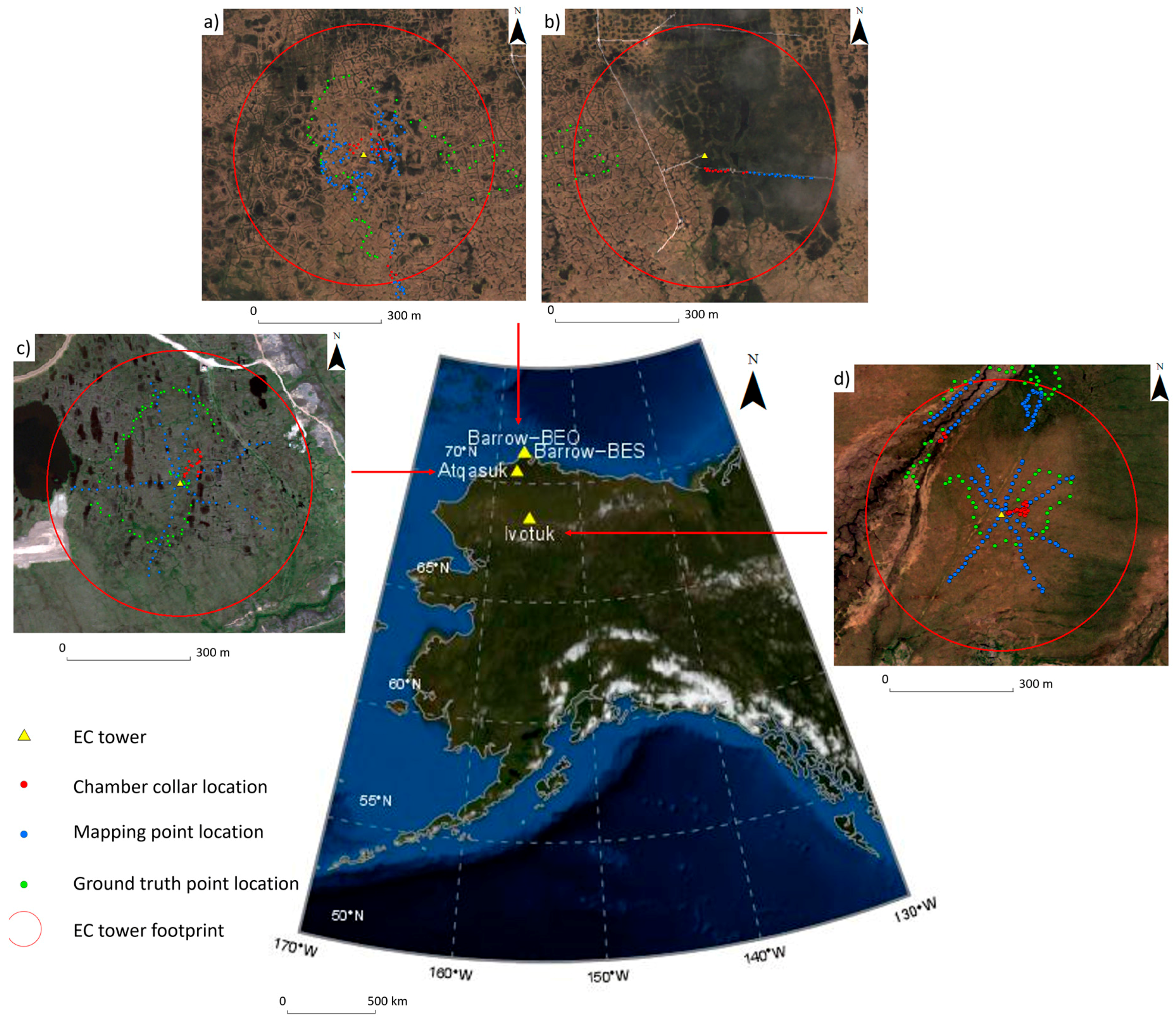
2.1. Site Description

This study was undertaken at four different field sites across the North Slope of Alaska, all of which have had CH4 fluxes quantified by EC towers and chambers and have had field spectral measurements undertaken in their different vegetation types. Two sites are located near Utqiaġvik (formally known as Barrow), within the Barrow Environmental Observatory (71°16′51.61″N, 156°36′44.44″W; Figure 1), one of them (henceforth referred to as Barrow-BEO) consists of highly-polygonal tundra, whereas the other (henceforth referred to as Barrow-BES) is situated in a vegetated drained lake basin [10]. The third site, Atqasuk (70°28′40″N, 157°25′05″W) is located at approximately 100 km south of the Barrow sites. This microtopography includes primarily low-centred, well-developed polygonal tundra with well-drained high edges [44,45]. The fourth site, Ivotuk (68.49°N, 155.74°W) is located in the foothills of the Brooks Range Mountains, approximately 300 km south of Barrow [10]. There is no substantial polygon formation located here, and the site mostly consists of a gentle northwest facing slope and wet meadow on the margins of a stream.
The Barrow-BEO/Barrow-BES EC tower height is approximately 2.2 m, with the Atqasuk and Ivotuk EC towers being approximately 2.3 m and 3.2 m tall, respectively. We represented the tower footprint as the circle of 300 m radius around the location of the EC tower [46,47] to allow for comparison between sites. This is the area we analysed for each study site as described below.

2.2. Remote Sensing Imagery

WorldView-2 multispectral imagery (2 m resolution) acquired for Barrow-BEO and Barrow-BES on the 25 July 2014, Atqasuk on the 9 July 2014 and Ivotuk on the 21 June 2013, were used in this study, corresponding to the closest date to the flux measurements, vegetation sampling, and field spectral measurement campaigns. The multispectral WorldView-2 data (eight sensor bands: coastal: 400–450 nm; blue: 450–510 nm; green: 510–580 nm; yellow; 585–625 nm; red: 630–690 nm; red edge: 705–745 nm; near-IR1: 770–895 nm; and near-IR2: 860–1040 nm) were georeferenced and calibrated to top-of-atmosphere (TOA) reflectance following the procedures outlined by Digital Globe (Digital Globe Corporate, Longmont, CO, USA). A dark object subtraction was also carried out on the satellite imagery in order to account for any atmospheric effects, such as haze or cloud cover, that may occur in the imagery [48]. This is a commonly-applied method for atmospheric correction achieved by calculating minimum radiance reflectance for each band in the image as the first percentile radiance value over the image (accounting for atmospheric effects such as haze) and is subsequently subtracted from all pixels [49,50].

2.3. Vegetation Data

Our analysis focused on mapping the dominant vegetation communities at the four different field sites (Table 1). Detailed vegetation community surveys were conducted in the field and the geographical location of the surveys was registered using dGPS (Trimble R7, Trimble Navigation Limited, Sunnyvale, CA, USA). In total we surveyed 130 locations for Barrow-BEO, 50 locations for Barrow-BES, 90 locations for Atqasuk, and 150 locations for Ivotuk [40] (shown as point locations in Figure 1). These data were used to train classifiers to map the dominant vegetation communities as detailed in the following sections.
At these locations, we collected detailed data on floristic composition which we used to determine vegetation communities using hierarchical one-way clustering and non-metric multidimensional (NMDS) analysis [40]. Eight communities were identified (see [40] for specific details of plant communities). The Barrow-BEO and Barrow-BES EC tower footprints contained three dominant vegetation communities. The mesic sedge-grass-herb meadow community is dominated by a combination of various graminoid species (including Eriophorum russeolum and Poa arctica), bryophytes, and lichens. The wet sedge meadow community contains mostly sedges, including Carex aquatilis and Sphagnum spp., and Drepanocladus spp. mosses. Finally, the dry lichen heath community consists of Polytrichum moss and various lichen species [40]. At Atqasuk, the EC tower footprint was made up of two dominant vegetation communities. The tussock tundra (non-sandy substrates) community is dominated by Eriophorum vaginatum (sedge tussock), interspersed with Rubus chamaemorus (forb) and Aulocomnion turgidum (moss). The wet sedge community here is dominated by Eriophorum angustifolium and Eriophorum russeolum. The EC tower footprint at Ivotuk is dominated by three vegetation communities. The tussock tundra (non-sandy substrates) is similar to Atqasuk, also containing Eriophorum vaginatum tussocks but interspersed with Sphagnum spp. moss, alongside various deciduous and evergreen shrubs. The wet sedge meadow community consists of tall Carex aquatilis, with large Salix pulchra shrubs and Sphagnum spp. moss carpet. Finally, the mixed shrub-sedge tussock community contained large Salix pulchra and Betula nana shrubs with Eriophorum vaginatum tussocks.
In addition to the vegetation surveys, ground-truthing points (GTPs) were collected to evaluate map accuracy. GTPs were collected across each of the tower footprint area following a non-probability sampling design [51]. One hundred GTPs were used at Barrow-BEO/Barrow-BES, 60 GTPs were used at Atqasuk and 70 GTPs were used at Ivotuk. See Figure 1 for the location of the GTPs used in the accuracy assessment. Due to Barrow-BES being extremely waterlogged, there was a limitation to the amount of GTPs that could be collected ‘randomly’ across this site as sampling had to be performed from a boardwalk, therefore, the majority of GTPs were collected across the same vegetation types to the west of the tower (between the Barrow-BEO and Barrow-BES towers).

2.4. Vegetation Mapping

Three classifiers were tested to map tundra vegetation within the tower footprint area at a 2 m scale, namely k-means, linear discriminant analysis (LDA), and random forest (RF). Mapping tundra vegetation has inherent challenges at different scales, but as we wanted to link the results to CH4 fluxes derived from both chamber and eddy covariance tower measurements, this seemed a reasonable scale of analysis. The methods were chosen because of their ability to discriminate among vegetation classes and likely can capture the tundra variability within the tower footprint. For example, Muster et al. [39], Langford et al. [41], and Moody et al. [52] have successfully used the k-means classifier to map tundra vegetation at the landscape scale. Bratsch et al. [53] have used LDA previously to distinguish between different lowland tundra types and it has also been used by Gong et al. [54] and Clark et al. [55], for example, to map different vegetation types across other ecosystem types. Finally, Chapman et al. [56] and Bradter et al. [57] have used the RF classifier to successfully map upland vegetation.
The k-means method was chosen as it is simple and easy to implement and differs from the previous two techniques, as it is an unsupervised classification algorithm, i.e., it does not require training data. However, it requires an arbitrary number of classes to be defined by the user [58]. A k-means unsupervised classifier algorithm [59] was applied to the WorldView-2 imagery for all field sites. K-means classification is an iterative clustering algorithm in which pixel values are assigned to a number of randomly-generated clusters, with the number of clusters defined by the user, based on the linear distance between cluster means [39,60]. First, we set the k-means algorithm to differentiate 10 classes using 100 iterations to create the initial vegetation map. This initial number of classes was higher than the known vegetation classes defined from the vegetation community analysis [40]. However, this was necessary in order to capture the variability within the landscape. We then grouped similar classes produced by the automated k-means to reduce the number of classes and to produce a post classification ‘smoothing’ that would approximate the known number of vegetation communities. For example, where the initial k-means classification may have indicated three or four areas that contain vegetation communities that have similar pixel values (different wet sedge species for example), these were grouped as one broad community. The criteria for grouping was based on previous research for these regions [40,61]. K-means was applied in ENVI (Exelis Visual Information Solutions, Boulder, CO, USA).
Both the RF and LDA methods are supervised classifiers and we used 70% of the GTPs to train these classifiers. The LDA method was chosen because it allows for the identification of significant differences among groups based on relatively large numbers of variables [62], through variable reduction to linear combinations of those variables that explain the majority of variation in the data [63]. The RF method is the most advanced and there are several advantages of using RF, as it is more robust to outliers and better at handling larger amounts of training data successfully [64]. Additionally, RF does not require that input variables are not affected by collinearity and, therefore, do not over-fit to noise within the dataset [56]. The RF classifier also produces estimations of variable importance, allowing for further analysis of specific input variable contribution within the classifier [65].
The RF classifier [66] was applied to the WorldView-2 imagery for all field sites. The RF classifier is a multiple decision tree classifier, based on classification and regression trees (CART; [67]). The algorithm searches across a randomly-selected subset of the input variables to determine a split at each node [68]. When the RF grows a tree, it uses the best split of the subset in the division of every node instead of using the best split variables [69]. This can reduce the strength of a single tree, but, overall, it reduces any generalisation error [66]. The output of the classifier is determined by a majority vote within the decision trees [65]. Cross-validation accuracy is calculated using the remaining training data (known as out-of-bag (OOB)) and used to evaluate the accuracy of the model before a formal accuracy assessment [70] which is described at the end of Section 2.4. In this study, 500 trees were grown as the more trees used, the more reliable estimates that can be produced from the OOB predictions [71]. The input variables used were the blue, red, and NIR bands of the WorldView-2 multispectral imagery as these bands are useful for distinguishing between different arctic tundra vegetation types [72]. For every tree produced, 2/3 of the data were used to create the classification tree and 1/3 of the data were used to validate the classification [72]. Random forest classification was performed using the ‘rgdal’, ‘raster’, ‘caret’, ‘randomForest’, ‘e1071’, and ‘snow’ packages in R version 3.3.2 (R Core Team 2016, Vienna, Austria).
We also used vegetation maps produced in our previous work using LDA [40]. To perform this analysis, field spectroscopy data (256 discrete bands ranging between 450 nm and 1040 nm) for each of the eight vegetation communities (Table 1) were collected using a UniSpec DC field spectrometer (PP Systems, Amesbury, MA, USA), at the four field sites during 2014 (Barrow-BEO n = 150 and Barrow-BES n = 30; 11 July 2014, Atqasuk n = 60; 29 July 2014 and Ivotuk n = 90; 16 July 2014). For specific details on data collection using the field spectrometer see Davidson et al. [40]. The spectroscopy data were rescaled to match the broad bands of WorldView-2 satellite imagery by averaging the band reflectance as follows; blue: 450–510 nm; green: 510–580 nm, yellow: 585–625 nm; red: 630–690 nm, red edge: 705–745 nm; near-IR1: 770–895 nm; and near-IR2: 860–1040 nm). These data were used to develop two LDA models to map vegetation per site, one with rescaled data and one with rescaled data plus three vegetation indices (VIs): the normalised difference vegetation index (NDVI; [73]), the normalised difference water index (NDWI; [74]), and the enhanced vegetation index (EVI; [75]). The VIs were used in combination with the rescaled reflectance data as they can relate to regions of the spectra that cannot be accounted for when analysing each broad band individually [40].
Overall classification accuracy was calculated for all the maps, as the number of ground truth points correctly classified as a given vegetation community divided by the total number of points in the field data for that vegetation community. Producers’ accuracy (total number of correct pixels in a category, divided by the total number of pixels of that category as derived from the ground truth points (omission error) and users’ accuracy (total number of correct pixels in a category, divided by the total number of pixels that were classified in that category (commission error)) [76] were also calculated for each vegetation community. The Kappa coefficient metric [77] was used as a statistical measure summarising the classification accuracy. The Kappa coefficient (K) is the proportion of actual agreement between classes after the chance agreement is removed from consideration [78]:
K = P o P c 1 P c
where Po is the proportion of observed agreements and Pc is the proportion of agreements expected by chance. Kappa coefficient values range from −1 to 1 (with <0 indicating no agreement and >0 fair to substantial agreement [77]). The agreement between the mapped distributions of vegetation communities was assessed by overlaying all the maps produced with the different methods and identifying pixels consistently classified as the same vegetation community and pixels which were not.

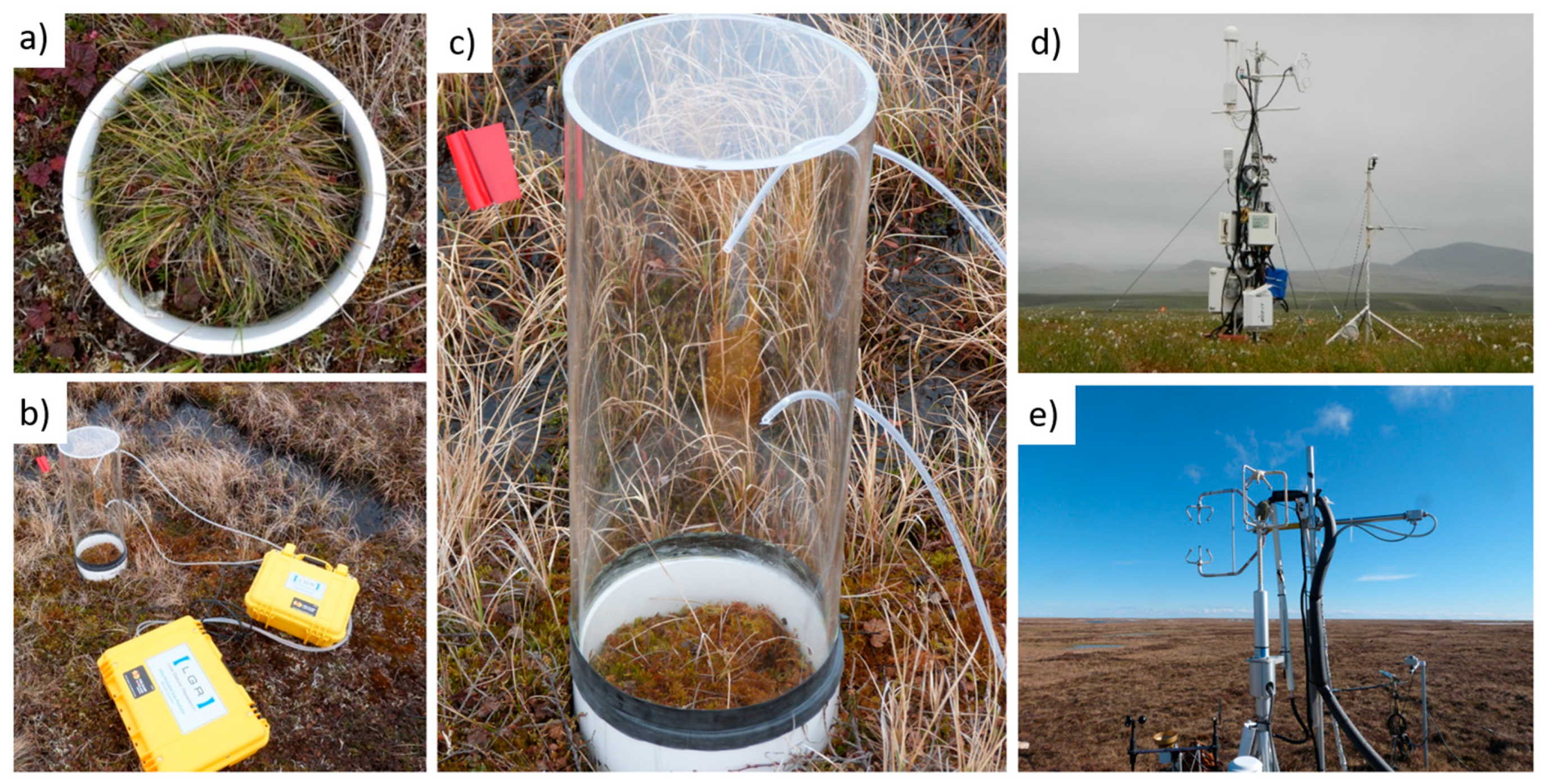
2.5. Measurements of CH4

To obtain data at the chamber level to upscale to the tower footprint, CH4 fluxes were measured at the four sites (Barrow-BEO, Barrow-BES, Atqasuk, and Ivotuk [9]) in each vegetation type using plastic replicate collars and a LGRTM, Ultraportable Gas Analyzer (UGGA), Model 951-0011 (Los Gatos, Research, Palo Alto, CA, USA). This was connected to a bespoke plexiglass chamber (500 mm height × 215 mm diameter) via inlet and outlet tubing. A total of six collars were placed in each vegetation community at the Barrow sites and seven collars were used at Atqasuk and Ivotuk within each vegetation community (Figure 2). Vegetation types at the plot level were amalgamated to match the vegetation communities described above and to carry out analysis at the patch scale (Table 1). Measurements took place once a week between 29 June and 22 August 2014 at Barrow-BEO/Barrow-BES, three times between 3 July and 13 August 2014 at Atqasuk, and three times between 22 June and 20 August 2014 at Ivotuk. Fluxes were measured between 11 am and 2 pm. Unfortunately, as the shrub community found at Ivotuk contained shrubs taller than 1 m, and the chamber used for measuring fluxes was only 50 × 20 cm, flux measurements could not be carried out in this community. The size of the chamber was appropriate for all other vegetation communities at this location. For mean CH4 flux for each vegetation community at each site, see Figure S1.
All four field sites had an EC tower measuring CO2 and CH4 emissions [18,45] (Figure 2). The Barrow-BEO/Barrow-BES and Atqasuk towers were equipped with a closed-path DLT-100 fast response CH4 analyser (Los Gatos Research, Mountain View, CA, USA) for continuous measurements of CH4 fluxes. At Ivotuk, due to limited power availability, a LI-7700 CH4 analyser (Li-Cor, Lincoln, Nebraska, USA) was used [10]. Half-hourly fluxes were calculated using the EddyPro software (www.licor.com/eddypro). De-spiking and absolute limit determination were included in the initial raw signal processing [79]. Any outliers found were discarded. Methane fluxes were gap-filled using an artificial neural network (ANN) [10]. The meteorological inputs into the ANN included variables such as air temperature, soil temperature (at 10 cm depth) and photosynthetic photon flux density (PPFD). The ANN was calculated 25 times and the median value gained was used to gap-fill at a half-hourly flux time resolution. For more detailed information, see Goodrich et al. [80] and Zona et al. [10]. As plot fluxes were measured between 11 am and 2 pm, the mean flux from the EC tower was taken between these times for further comparisons with the upscaled plot fluxes.

2.6. Upscaling CH4 Emissions

Several methods have been developed to upscale CH4 fluxes, which often rely on the areal fraction of the vegetation community distribution around the EC tower [30]. The area-weighted average method uses the areal fraction of a vegetation community within a given area and multiplies it by CH4 emissions derived from chamber measurements [33,81,82]. Other methods, such as the footprint-weighted average technique, upscale CH4 fluxes by using a 2-D footprint model and weight the CH4 emission potential within a given fetch of the EC tower footprint with the area of each vegetation community being defined by the model rather than from previously-produced maps [30]. We tested two methods: a non-weighted and a footprint-weighted areal estimate of CH4 fluxes.
The non-footprint weighted method, is a simple area-weighted average method previously used in several studies’ upscaling of CH4 emissions across arctic tundra ecosystems [30,33,81,82]. It was chosen as it allowed for the inclusion of detailed community distribution information in the upscaling process and due to the limited temporal resolution of the plot-level flux measurements. The upscaled flux is calculated using the following equation:
Up_flux = plot flux × area/total area
where Up_flux is the upscaled plot flux, plot flux is the mean plot-derived CH4 flux for a given community on a given date, area is the area of vegetation community in m2 in the EC tower footprint, and total area is the EC tower footprint. We also upscaled fluxes using the specific dominant wind direction at each site on each date between 11 am and 2 pm in order to see if this improved the upscaling. This was done in a similar manner as before, but only using the areal fraction of vegetation communities within the wind direction (wind direction for each site ranged between 30° and 215° at Barrow-BEO/Barrow-BES, 60° and 180° at Atqasuk and 50° and 200° at Ivotuk, dependent on the measurement date).
The chosen footprint-weighted method was the two-dimensional analytic footprint model [46]. The model was applied to the half-hourly EC data to produce half-hourly footprints in the form of a raster grid with a resolution of 1 m2. EC data was filtered with standard methods [10] with the addition of filtering out any measurements which fell outside of the maximum fetch (the furthest distance the tower observes). The half-hourly footprints were combined to give an average footprint which was used to calculate percent footprint contribution of each of the vegetation classes for each time period. The vegetation community areal fractions derived from the LDA classifier were used in the footprint analysis as this method produced the most accurate maps. The 29 June 2014 measurement date for Barrow-BEO/Barrow-BES were removed from the analysis because the uStar value was too low (uStar < 0.2). Similarly, all measurements dates from Ivotuk were removed as they did not meet the atmospheric stability quality control criteria (qu_ch4 > 1). In both of these cases the footprint output is deemed unreliable. The output of the model produced a percentage of the potential CH4 emission from each vegetation community. This was then used to upscale the chamber fluxes using the same method as described previously. Since wind speed and direction were already included in the footprint model there was no need to further test for their effects.
Upscaled CH4 fluxes from both the non-weighted and the footprint-weighted areal estimate methods were then compared to the measurements from the EC towers for each site using the Pearson correlation coefficient. We checked whether there were influential outliers within the raw data and the upscaled dataset using Cook’s distance [83] (Figure S2). Cook’s distance is a measurement of each observations leverage and residual values. It is calculated by summarising how much all the values in the coefficient model change when the influential (outlier) observation is removed. When a Cook’s distance value is more than three times the mean value, this indicates it is an influential outlier [83]. This analysis was performed because of the nature of CH4 release, where natural ebullition events can occur unpredictably. These could potentially be enhanced when placing the chamber onto the flux collar and causing pressure on the ground that artificially stimulates an ebullition event and, thus, CH4 fluxes after these might be biasing the statistical analysis. All statistical analysis was done using R version 3.3.2 (R Core Team 2016, Vienna, Austria).

3. Results

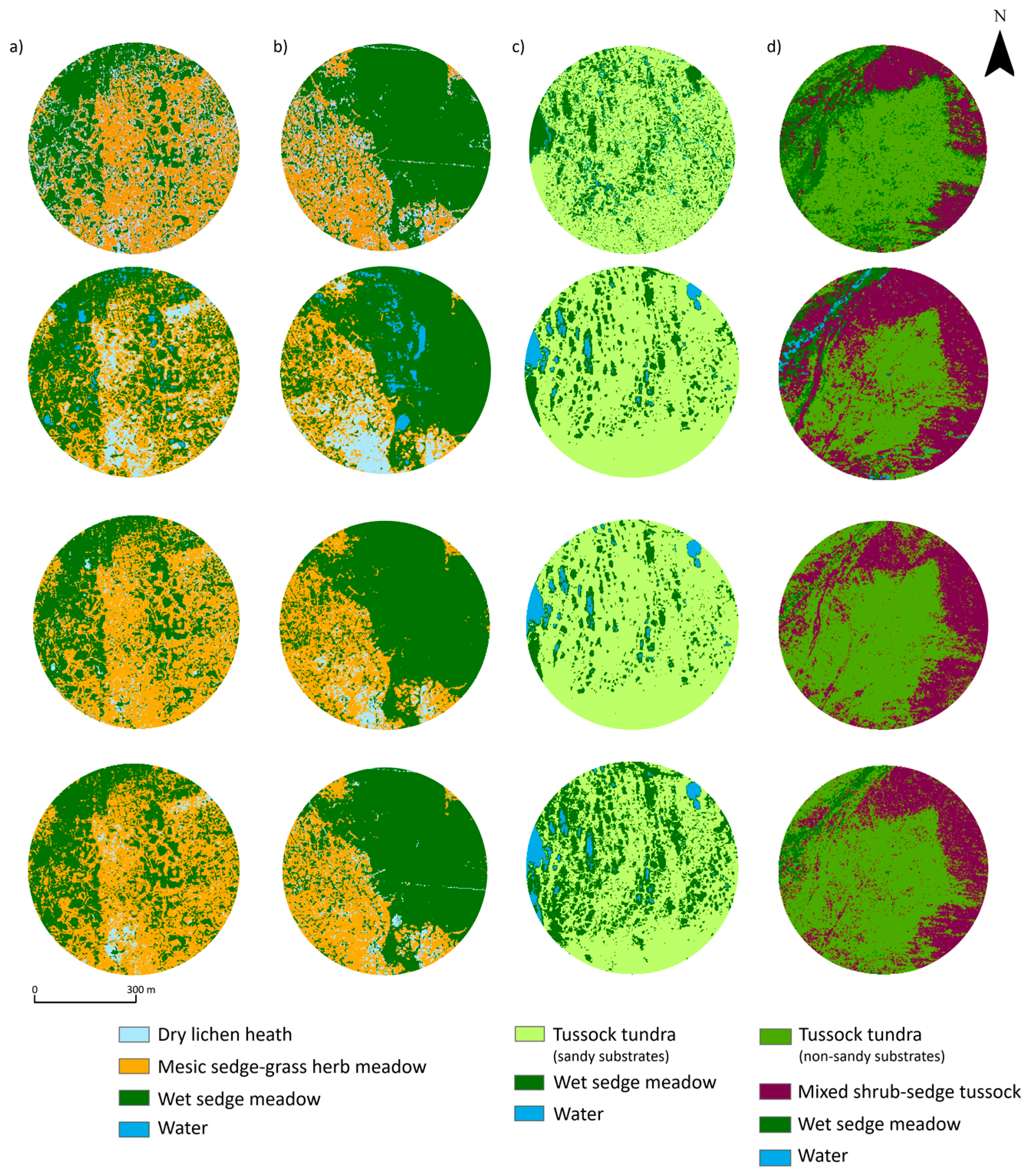
3.1. Mapping Tundra Vegetation

The LDA mapping method produced better maps than the other methods (except for Ivotuk), with higher classification accuracies between 60% and 80% (Table 2). Including vegetation indices decreased the classification accuracy, except for Ivotuk (Table 2). The random forest method produced accuracies similar to those of the LDA including VIs. The k-means method produced accuracies within the same range as LDA, although slightly lower per site, again except for Ivotuk.
Atqasuk was best mapped across all methods, with 97% and 70% of pixels correctly classified as tussock tundra and wet sedge meadow using LDA (Table S1). Barrow-BEO/Barrow-BES sites were the most difficult to map, with classification accuracies varying between 40% and 77% (Table S2). At Ivotuk, classification accuracies for each vegetation type ranged from between 21% and 98%, depending on which method was chosen (Table S2). The highest accuracies were reached for wet sedge meadow and tussock tundra communities (>80%) while the dry lichen heath was very poorly classified (27–50%; Table S2) overall.
The greatest agreement between maps occurred between the LDA and LDA with VIs at Barrow-BEO/Barrow-BES and Ivotuk whereas, at Atqasuk, the greatest agreement occurred between the LDA and k-means (94.8%). The largest disagreement in mapped vegetation was between k-means and RF maps at both Barrow sites (78.1% and 33.7%, respectively). At Atqasuk and Ivotuk the largest disagreements occurred between LDA with VIs and RF, and k-means and RF, respectively (Table S3).
Overall, the footprint around the Barrow-BEO EC tower was covered by about 50% of mesic sedge-grass-herb meadow and 42–47.1% of wet sedge meadow tundra, and only 3–10% dry lichen heath towards the southeast of the EC tower (Table 3). With similar vegetation communities, wet sedge meadow dominated Barrow-BES (>60%) (Figure 3; Table 3). Atqasuk EC tower footprint is largely dominated by tussock tundra (>80%; Figure 3, Table 3. Finally, the footprint of the Ivotuk EC tower consists of mostly non-sandy tussock tundra (60%; Table 3), while mixed shrub-sedge tussock tundra occupies 18.3–46.5% (Figure 3; Table 3). Table S2 shows the vegetation community in m2 for each mapping technique.

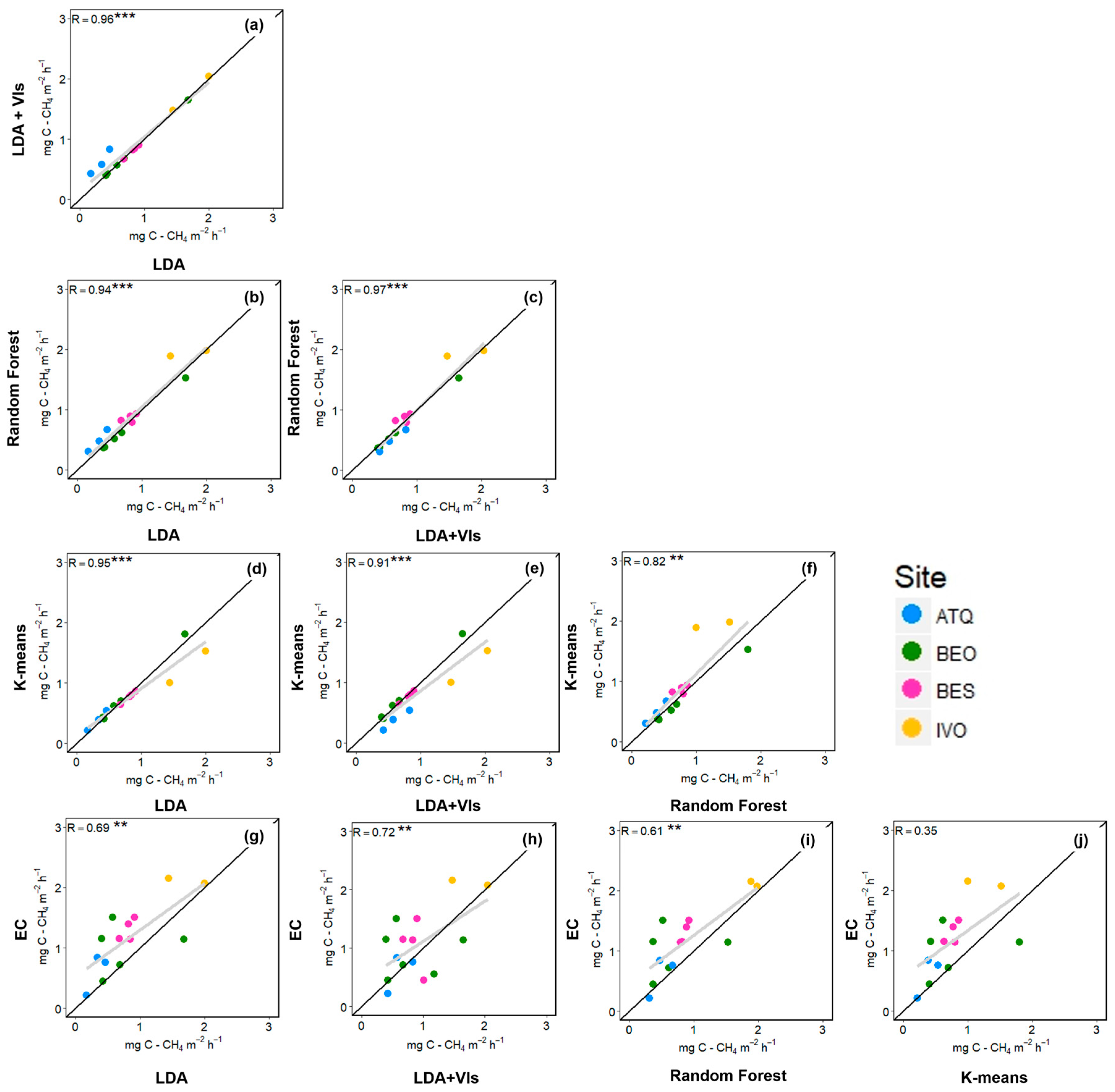
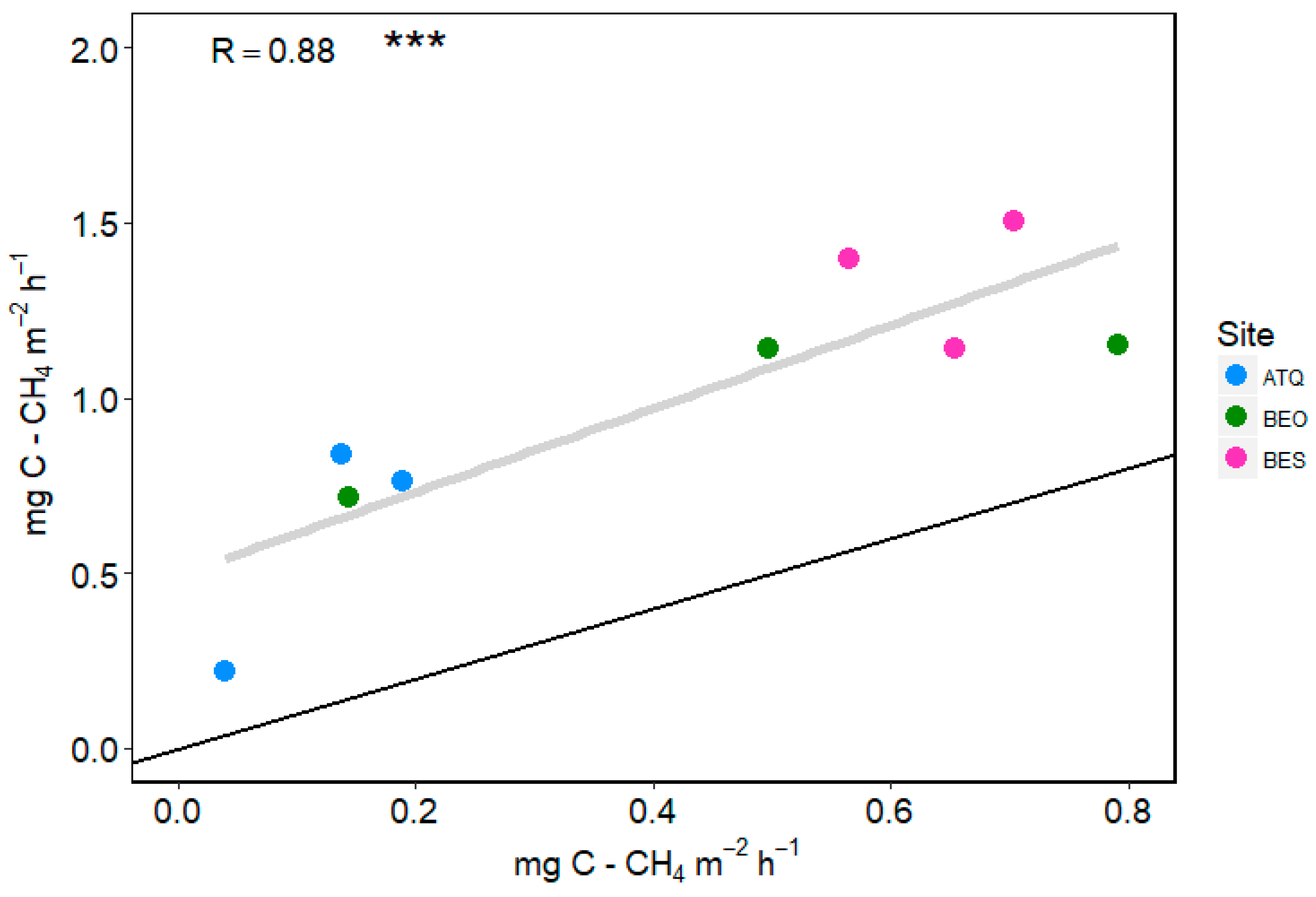
3.2. Upscaling CH4 Emissions

Most non-footprint weighted upscaling calculations based on the four different maps estimated approximately 1 mg C-CH4 m−2 h−1 more CH4 than the measurements obtained with the EC tower. We found a significant positive correlation between non-footprint-weighted upscaled fluxes and the EC tower, between 0.52 and 0.62 after removing outliers (Figure 4, see the Supplementary Material for a detailed description of the identification of outliers, Figure S3 and for comparison between upscaled fluxes and EC towers including outliers, Figure S4). At a few dates for Barrow-BES, the upscaling method underestimated the flux by approximately the same amount (1 mg C-CH4 m−2 h−1) (Table S4). All the non-footprint-weighted upscaled results showed either over or underestimation of fluxes with no consistent direction in the difference between the mapping methods, except for LDA including VIs at Atqasuk (Table S5). LDA and LDA including VIs tended to have smaller overestimates of CH4 fluxes in comparison to the other methods. We did, however, find a highly significant correlation between each of the non-footprint-weighted upscaling comparisons (correlation coefficients ranging between 0.91 and 0.97; Figure 4).
Using the footprint-weighted upscaling method improved the relationship between upscaled chamber CH4 fluxes and EC tower measurements (Figure 5), and the correlation coefficient between the footprint-weighted upscaling fluxes and the eddy covariance fluxes was 0.88 (p-value = 0.0007). This was a 20–30% improvement on the predictive power of the non-footprint-weighted upscaling method. This result was consistent for all sites, except for Ivotuk for which no footprint-weighted upscaling was produced.

4. Discussion

Across four heterogeneous arctic tundra locations, we have assessed the potential of using remotely-sensed vegetation distribution maps to upscale plot-level CH4 fluxes and compare to EC tower flux measurements using both a non-footprint weighted and a footprint-weighted upscaling method. We show that the most accurate vegetation distribution maps were produced using LDA, although, in general, all classifiers agreed in the distribution of the most dominant communities at each site. Importantly, probably because of the high agreement between vegetation distribution maps across classifiers despite the differences in accuracy, the classifier had a minimal impact on the upscaling of the fluxes. Generally, upscaled CH4 emission estimates showed a significant positive correlation with the EC tower measurements for both weighting methods, with increased performance of the footprint-weighted method. These results highlight the ability to upscale CH4 flux from chamber to tower footprint scales by including accurate vegetation community distribution maps. These results also suggest that the spatial heterogeneity of the tundra ecosystems has a strong impact on the potential CH4 flux, and should be taken into account when extrapolating small-scale measurements to larger ecosystem scales.

4.1. Tundra Vegetation Mapping

Mapping arctic tundra vegetation is very challenging due to the enormous heterogeneity present over a few meters ([39,43,84]. Not only can the variability of the vegetation make mapping more difficult, but the substantial cloud cover in the Arctic can decrease the number of available images that can be used for this excersise [85]. The limited imagery available might reduce the chances of an overlap between the dates of ground level and satellite data resulting in discrepancies in the phenological status of the vegetation in each of these datasets. The date of the satellite imagery used in this study was chosen to be as close as possible to the dates of the site level flux measurements and field spectroscopy measurements. Luckily this was possible for most sites, with the exception of Ivotuk, where no suitable imagery was available during the entire 2014 growing season. We were forced to use an image from 2013 at a similar time in the season so that the vegetation communities were at a similar phenological stage, but different years can have different environmental conditions, such as air temperature or date of snow melt, for example, adding to the challenges of this analysis.
The different techniques used to map the vegetation communities within the EC tower footprints had classification accuracies ranging between 54% and 91% (the agreement between each technique was also consistently greater than 60%), but LDA (closely followed by the RF technique) produced the most accurate vegetation communities distribution map. This suggests that mapping tundra vegetation is very dependent on having good training data to inform the classifier rather than using unsupervised algorithms. Yet, the k-means classifier provided the best classification accuracy for Ivotuk, which could arguably be described as the most spatially heterogenous of all the analyzed sites. However, the 2 m resolution of the WorldView-2 imagery was insufficient to capture this, therefore, the tussock tundra and moss-shrub community had to be combined. This simplification of the classes meant there were only three communities that covered large areas of the footprint allowing for a high classification accuracy to be derived. These types of issues were also highlighted by Parmentier et al. [82] who used a maximum likelihood classifier with GeoEye-1 data over Siberia. Other data products, such as aerial imagery obtained through the use of drones or LiDAR-derived digitial elevation models (DEMs), could be used to resolve this issue [86,87] as they could also account for variability within the local microtopography. However, Bartsch et al. [43] note that even coarse resolution maps can have value, especially in carbon/upscaling studies, and drones or LiDAR-derived digitial elevation models (DEMs) are expensive to collect and cannot be easily collected over large areas.
Nonetheless, all classifiers agreed in the dominance of wet sedge meadow at Barrow-BEO and Barrow-BES, and the tussock tundra communities for Atqasuk and Ivotuk. The wet sedge meadow community distribution differed from other techniques when using the LDA including VIs at Atqasuk, and the distribution of dry lichen heath at the Barrow sites also differed between mapping techniques. The difference in wet sedge meadow distribution could be attributed to the inclusion of VIs picking up differences in productivity across sites or reducing spectral noise as transformations of band reflectance can be less sensitive to external variables [88]. Although the dry lichen heath and the mesic sedge-grass herb meadow communities are physiognomically similar (though proportions of each species differ), their spectral profiles are significantly different from each other, especially in the red region around 630–690 nm [40]. Forbrich et al. [28] note that the greatest variability within their study is caused by variation of the source area vegetation composition.
The small number of vegetation communities present in the EC tower footprints can be useful to explain other ecological processes, such as carbon flux rates. If more classes were used, then a simplified understanding of their influence on such processes would be lost. The small number of classes presented in this study still provide valuable information and could be integrated into large multi-scale studies and models in the future [39]. Our previous research [9] indicated that vegetation type alone could explain over 50% of the variability of CH4 emissions across different tundra landscapes. By classifying only two or three vegetation communities (which showed strong differences of their potential flux at the plot scale), it allows for a clear understanding in which communities have the greatest influence on any flux measured at the patch scale.

4.2. Upscaled Flux Chamber Measurements

The upscaled CH4 emissions using both the non-footprint weighted and the footprint weighted methods showed a significant positive correlation with EC tower measurements, irrespective of the mapping method when outliers were removed. The potential origin of these outliers could be linked to ebullition events during the measurement period or an artefact of disturbance around the collar during the measurement period, although this was avoided as much as possible. Other upscaling studies that used vegetation community distribution using the non-footprint-weighted upscaling method [15,33] also had strong correlations between the upscaled fluxes and the EC tower fluxes. This could be because despite the variability in mapping method accuracy, all methods were quite consistent in predicting dominant vegetation types. It is well documented that vegetation has an important role in controlling CH4 emissions, through acting as a substrate for methanogenesis [16,17] and transporting CH4 from belowground to the atmosphere through a process called plant-mediated transport [21,22,89]. However, using a non-footprint weighted method to upscale fluxes is not always successful, as shown by Budischev et al. [30], who achieved a low correlation (0.14) between upscaled and EC fluxes, improving these results with the inclusion of a footprint analysis. Parmentier et al. [83] found good agreement between upscaled and EC tower emissions at the same site, indicating that temporal variations (both within and between years) will have a strong influence on the upscaled results. Our results support the use of a footprint-weighted upscaling method to more accurately upscale the chamber flux measurements. However, there was not a 1:1 relationship between upscaled fluxes using the footprint model and the EC towers, indicating that this methodology may underestimate the overall flux, the opposite to Budischev et al. [30], who showed the footprint model method produced a slight overestimation of the flux in comparison to the EC towers, attributed to localised differences in environmental conditions across the measurement period and vegetation classification error. Maruschak et al. [90] also upscaled chamber measurements aross a sub-arctic tundra ecosystem, using a high-resolution vegetation map and weighting the fluxes by their relative area. They found that this method again indicated an overestimation of the chamber measurements in comparison to the EC towers. They noted that the plots chosen for chamber measurements had a higher leaf area index (LAI) in comparison to similar areas in the region. By correcting for the higher LAI in the measurement plots, they found a tighter relationship between upscaled chamber measurements and the EC towers.
To improve upscaling estimates, understanding the phenological dynamics of the vegetation communities present could be useful, rather than just the spatial variation at one point in time [91,92]. It is interesting to see how much of an impact ‘drier’ sedge communities can have on the flux (between 10% and 38% of the measured flux) [9], further highlighting how different vegetation communities may contribute to CH4 budgets and their variability [30,91]. The use of automatic chambers could potentially bridge the gap between EC tower measurements and spatial chamber measurements as they provide detailed flux measurements with a better temporal resolution [93]. Care should be taken, however, when using chamber measurements, as they can can have lower emission values in comparison to EC towers due to the removal of the influence of wind by isolating the land surface [94].
Although we found a positive correlation between upscaled CH4 estimates and those derived from the EC towers, we found differences in emission estimates on a day to day basis (Table S4), which could be due to variation between vegetation community distribution and localised environmental variables such as water table depth or soil moisture, which could all equally influence CH4 flux [5,18,89]. Site-specific conditions can impact the relationship between upscaled and EC methods of measuring CH4 fluxes [95]. For example, at Barrow-BEO, upscaled emission values are similar to those measured by the EC tower, but this similarity deteriorates as the growing season progresses (Table S4). This could be due to the plants having a more significant impact on the fluxes in the earlier part of the season, but as the season progresses, other environmental variables, such as active layer thaw depth take over as the dominant control on CH4 fluxes [96]. This is in contrast with the Ivotuk site, where upscaled fluxes gradually become more comparable with the flux tower values (Table S4). As the growing season continues at the Ivotuk site, the influence of the tussock tundra community on the upscaled CH4 flux becomes much more comparable with the wet sedge meadow community. However, we must note that there were no wet sedge meadow collars in place on the 22 June 2014 due to this area of footprint being under water. It is possible that had we managed to include this area in the upscaling analysis for this date, upscaled emission values may have been more comparable with the EC tower. The inclusion of these collars on the second and third visit has a sizeable influence on the upscaled fluxes as they become more comparable to the EC measurement.
Although there is a disagreement on certain dates between the upscaled fluxes and the EC tower, it does not imply that the upscaling values are necessarily incorrect. Although EC towers have a better temporal resolution than spatial chambers, they may not represent the landscape sufficiently. On the other hand, spatial chamber measurements may not completely capture the large spatial variability of the tower footprint [15,28]. Our results suggest that care must be taken when extrapolating such results to a wider area. If the EC tower footprint is representative of the wider landscape then it could prove useful [30]. Alternatively, Sachs et al. [15] noted that Heikkinen et al. [12] extrapolated both chamber and EC measurements to a 114 km2 catchment, and then further still to a 205,000 km2 scale, but accuracy is quickly lost and budgets cannot be readily verified. Many upscaling studies calculate the flux uncertainty based on spatial and temporal variability of chamber measurements, but Bubier et al. [97] note that there is difficulty in combining both types of error. Our results are promising and provide evidence that these simple techniques can be useful for identifying the probability of CH4 emissions as linked to spatial and temporal variability within the flux tower footprints [98].

5. Conclusions

This study tests the applicability of using high-resolution multispectral satellite imagery and a variety of mapping techniques to provide fine-scale vegetation maps to upscale CH4 fluxes at four Alaska tundra EC tower sites. Our results provide evidence that upscaling is successful, as long as the major vegetation communities are appropriately mapped. Our study shows that the LDA mapping method produced the best across-site classification accuracies of the vegetation comunities, but also that using very different mapping methods had a minimal influence on the upscaling. These results highlight the importance in including vegetation community data in upscaling exercises and regional-scale CH4 budget models, and further strengthen the idea that the high spatial heterogeneity of the tundra ecosystems has a strong impact on the potential CH4 fluxes. As shown by our previous research, CH4 emissions across these sites are controlled by environmental conditions, such as the water table depth, as well as the specific vegetation types present at the plot scale. The results could be improved even further by using more sophisticated upscaling methodologies, such as high-resolution footprint modeling, including a combination of vegetation community distribution and different environmental parameters, but also by including more information on vegetation phenology to better link fluxes with vegetation function. Although the vegetation maps produced here have shown they can successfully be used to upscale to a 300 m EC tower footprint, we suggest that care needs to be taken when extrapolating such results to a wider region. Agreement between upscaled estimates at fine spatial and temporal scales was not always consistent, suggesting that other factors may be at play, such as localised microtopographical or meteorological conditions. Further use of novel remote sensing products will continue to provide valuable data for improving upscaling relations and examining the patterns and dynamics of arctic tundra vegetation communities and their impact on potentially increasing CH4 emissions.

Supplementary Materials

The following are available online at www.mdpi.com/2072-4292/9/12/1227/s1, Supplementary material: Figure S1. CH4 flux (mg C-CH4 m−2 h−1) for each vegetation community at (a) Barrow-BEO/Barrow-BES (six measurements between 29 June and 22 August 2014, (b) Atqasuk (three measurements between 3 July and 13 August 2014), and (c) Ivotuk (three measurements between 22 June and 20 August 2014). At Barrow-BEO/Barrow-BES: DLH is dry lichen heath (n = 37), MS is mesic sedge-grass-herb meadow (n = 65), WSM is wet sedge meadow (n = 101). At Atqasuk: TT is tussock tundra (sandy substrates) (n = 42), WSM is wet sedge meadow (n = 20). At Ivotuk: TT is tussock tundra (non-sandy substrates) (n = 46), WSM is wet sedge meadow (n = 10). Boxplots represent median (midline), quartiles (box), and maximum and minimum (whisker) with outliers represented as black points. Figure S2. The error between mapping techniques (shown in red): (a) Barrow-BEO; (b) Barrow-BES; (c) Atqasuk; and (d) Ivotuk. Figure S3. Diagnostic plots looking influential observations defined by Cook’s Distance. Red line is the cut-off line, with values above this line being deemed influential. Figure S4. Comparisons between upscaling techniques (a–f) and between upscaling technique and eddy covariance tower measurements (g–j) with no outliers removed. R is the correlation coefficient and *** denotes significance, p < 0.001, ** denotes significance, p < 0.01, * denotes significance, p < 0.05. The black line shows a 1:1 relationship and the grey line is the linear regression. Table S1. Percentage of vegetation community distribution for each mapping technique. N/A denotes community was not present. linear discriminant analysis (LDA), Linear discriminant analysis, including vegetation indices (LDA + VIs), K-means (KM), and random forest (RF). Table S2. Vegetation community distribution in m2 for each mapping technique. N/A denotes community was not present. Table S3. Percentage difference between the EC tower flux measurements and the upscaled chamber flux measurements for each measurement date. Values are rounded to nearest whole number. Table S4. Upscaled methane (CH4) fluxes assuming a constant vegetation and using the distribution of each vegetation community from the four mapping methods and associated eddy covariance tower flux measurement for each date. VIs indicates the vegetation indices–normalized difference vegetation index (NDVI), normalized difference water index (NDWI), and enhanced vegetation index (EVI). EC indicates eddy covariance. N/A denotes that the upscaled flux could not be calculated. Table S5. Absolute difference between the EC tower flux measurements and the upscaled chamber flux measurements for each measurement date. Values are rounded to two decimal places. Negative values indicate the upscaled chamber flux was greater than those derived from the EC tower. Percentage difference is shown in parenthesis with values rounded to nearest whole number.

Acknowledgments

This work was funded by the Office of Polar Programs of the National Science Foundation (NSF) awarded to DZ, and WCO (award numbers 1204263 and 1702797) with additional logistical support funded by the NSF Office of Polar Programs, and by the Carbon in Arctic Reservoirs Vulnerability Experiment (CARVE), an Earth Ventures (EV-1) investigation, under contract with the National Aeronautics and Space Administration, and by the ABoVE (NNX15AT74A; NNX16AF94A) program. This research was conducted on land owned by the Ukpeagvik Inupiat Corporation (UIC). We would like to thank the Global Change Research Group at San Diego State University, and UMIAQ and UIC for logistical support. This project has also received funding from the European Union’s Horizon 2020 research and innovation program under grant agreement no. 727890, and from a NERC grant (award number NE/P002552/1) to DZ and WCO and the CYCLOPS grant (NE/K00025X/1) awarded to GKP. SJD is supported by a NERC PhD studentship. This research was conducted on land owned by the Ukpeagvik Inupiat Corporation (UIC). We would like to thank the Global Change Research Group at San Diego State University in particular Patrick Murphy and UMIAQ and UIC for logistical support Ali Hoy, and Owen Hayman for the help in the field. We would like to thank Cole Kelleher and the team at the Polar Geospatial Centre at the University of Minnesota for their help with the satellite imagery. We’d also like to thank Koen Hufkens for providing the base ‘blue’ marble raster shown in Figure 1. We thank the anonymous referees and the editor for their constructive comments on our manuscript.

Author Contributions

D.Z., W.C.O. and G.K.P. secured the funding; S.J.D., M.J.S., V.L.S., D.Z., W.C.O. and G.K.P. designed the study; S.J.D. and V.L.S. performed the research; S.J.D. and M.J.S. analysed the data with input from V.L.S., D.Z., K.R.S. and G.K.P.; and S.J.D., M.J.S., G.K.P. and D.Z. wrote the paper.

Conflicts of Interest

The authors declare no conflict of interest.

References

  1. Intergovernmental Panel on Climate Change (IPCC). Climate Change: The Physical Science Bases; Cambridge University Press: Cambridge, UK, 2013. [Google Scholar]
  2. Christensen, T.R. Methane emissions from Arctic tundra. Biogeochemistry 1993, 2, 117–139. [Google Scholar] [CrossRef]
  3. McGuire, A.D.; Christensen, T.R.; Hayes, D.; Heroult, A.; Euskirchen, E.; Kimball, J.S.; Koven, C.; Lafleur, P.; Miller, P.A.; Oechel, W.; et al. An assessment of the carbon balance of Arctic tundra comparisons among observations, process models and atmospheric inversions. Biogeosciences 2012, 9, 3185–3204. [Google Scholar] [CrossRef] [Green Version]
  4. Dlugokencky, E.J.; Nisbet, E.G.; Fisher, R.; Lowry, D. Global atmospheric methane: Budget, changes and dangers. Philos. Trans. R. Soc. Lond. A 2011, 369, 2058–2072. [Google Scholar] [CrossRef] [PubMed]
  5. Olefeldt, D.; Turetsky, M.R.; Crill, P.M.; McGuire, A.D. Environmental and physical controls on northern terrestrial methane emissions across permafrost zone. Glob. Chang. Biol. 2013, 19, 589–603. [Google Scholar] [CrossRef] [PubMed]
  6. Yvon-Durocher, G.; Allen, A.P.; Bastviken, D.; Conrad, R.; Gudasz, C.; St-Pierre, A.; Thanh-Duc, N.; del Giorgo, P.A. Methane fluxes show consistent temperature dependence across microbial to ecosystem scales. Nature 2014, 507, 488–495. [Google Scholar] [CrossRef] [PubMed]
  7. Oechel, W.C.; Vourlitis, G.L.; Hastings, S.J.; Zulueta, R.C.; Hinzman, L.; Kane, D. Acclimation of ecosystem CO2 exchange in the Alaskan Arctic in response to decadal climate warming. Nature 2000, 406, 978–981. [Google Scholar] [CrossRef] [PubMed]
  8. Chapin, F.S.; Sturm, M.; Serreze, M.C.; McFadden, J.P.; Key, J.R.; Lloyd, A.H.; McGuire, A.D.; Rupp, T.S.; Lynch, A.H.; Schimel, J.P.; et al. Role of land-surface changes in arctic summer warming. Science 2005, 310, 657–660. [Google Scholar] [CrossRef] [PubMed]
  9. Davidson, S.J.; Sloan, V.L.; Phoenix, G.K.; Wagner, R.; Fisher, J.P.; Oechel, W.C.; Zona, D. Vegetation type dominates the spatial variability in CH4 emissions across multiple Arctic tundra landscapes. Ecosystems 2016, 19, 1116–1132. [Google Scholar] [CrossRef]
  10. Zona, D.; Gioli, B.; Commane, R.; Lindaas, J.; Wofsy, S.C.; Miller, C.E.; Dinardo, S.J.; Dengel, S.; Sweeney, C.; Karion, A.; et al. Cold season emissions dominate the Arctic tundra methane budget. Proc. Natl. Acad. Sci. USA 2016, 113, 40–45. [Google Scholar] [CrossRef] [PubMed]
  11. Dinsmore, K.J.; Drewer, J.; Levy, P.E.; George, C.; Lohila, A.; Aurela, M.; Skiba, U.M. Growing season CH4 and N2O fluxes from a subarctic landscape in northern Finland from chamber to landscape scale. Biogeosciences 2017, 14, 799–815. [Google Scholar] [CrossRef]
  12. Heikkinen, J.E.P.; Virtanen, T.; Huttunen, J.T.; Elsakov, V.; Martikainen, P.J. Carbon balance in East European tundra. Glob. Biogeochem. Cycles 2004, 18, GB1023. [Google Scholar] [CrossRef]
  13. Petrescu, A.M.R.; van Beek, L.P.H.; van Huissteden, J.; Prigent, C.; Sachs, T.; Corradi, C.A.R.; Parmentrier, F.J.W.; Dolman, A.J. Modeling regional to global CH4 emissions of boreal and arctic wetlands. Glob. Biogeochem. Cycles 2010, 24, GB4009. [Google Scholar] [CrossRef]
  14. Melton, J.R.; Wania, R.; Hodson, E.L.; Poulter, B.; Ringeval, B.; Spahni, R.; Bohn, T.; Avis, C.A.; Beerling, D.J.; Chen, G.; et al. Present state of global wetland extent and wetland methane modelling: Conclusions from a model inter-comparison project (WETCHIMP). Biogeosciences 2013, 10, 753–788. [Google Scholar] [CrossRef]
  15. Sachs, T.; Giebels, M.; Boike, J.; Kutzbach, L. Environmental controls on CH4 emission from polygonal tundra on the microsite scale in the Lena river delta, Siberia. Glob. Chang. Biol. 2010, 16, 3096–3110. [Google Scholar] [CrossRef]
  16. King, J.Y.; Reeburgh, W.S.; Regli, S.K. Methane emission and transport by arctic sedges in Alaska: Results of a vegetation removal experiment. J. Geophys. Res. 1998, 103, 29083–29092. [Google Scholar] [CrossRef]
  17. Ström, L.; Ekberg, A.; Mastepanov, M.; Christensen, T.R. The effect of vascular plants on carbon turnover and methane emissions from a tundra wetland. Glob. Chang. Biol. 2003, 9, 1185–1192. [Google Scholar] [CrossRef]
  18. Zona, D.; Oechel, W.C.; Kochendorfer, J.; Paw, U.K.T.; Salyuk, A.N.; Olivas, P.C.; Oberbaeur, S.F.; Lipson, D.A. Methane fluxes during the initiation of a large-scale water table manipulation experiment in the Alaskan Arctic tundra. Glob. Biogeochem. Cycles 2009, 23, 1–11. [Google Scholar] [CrossRef]
  19. King, J.Y.; Reeburgh, W.S.; Thieler, K.K.; Kling, G.W.; Loya, W.M.; Johnson, L.C.; Nadelhoffer, K.J. Pulse-labelling studies of carbon cycling in Arctic tundra ecosystems: The contribution of photosynthates to methane emission. Glob. Biogeochem. Cycles 2002, 16, 1–8. [Google Scholar] [CrossRef]
  20. Christensen, T.R.; Ekberg, A.; Ström, L.; Mastepanov, M.; Panikov, N.; Öquist, M.; Svensson, B.H.; Nykänen, H.; Martikainen, P.J.; Oskarsson, H. Factors controllong large scale variations in methane emissions from wetlands. Geophys. Res. Lett. 2003, 30, 1414. [Google Scholar] [CrossRef]
  21. Bubier, J.L.; Moore, T.R.; Bellisario, L.; Comer, N.T.; Crill, P.M. Ecological controls on methane emissions from a northern peatland complex in the zone of discontinuous permafrost, Manitoba, Canada. Glob. Biogeochem. Cycles 1995, 9, 455–470. [Google Scholar] [CrossRef]
  22. Schimel, J.P. Plant transport and methane productions as a control on methane flux from arctic wet meadow tundra. Biogeochemistry 1995, 28, 183–200. [Google Scholar] [CrossRef]
  23. Fletcher, B.J.; Gornall, J.L.; Poyatos, R.; Press, M.C.; Stoy, P.C.; Huntley, B.; Baxter, B.; Phoenix, G.K. Photosynthesis and productivity in heterogeneous arctic tundra: Consequences for ecosystem function of mixing vegetation types at stand edges. J. Ecol. 2012, 100, 441–451. [Google Scholar] [CrossRef] [Green Version]
  24. Koelbener, A.; Ström, L.; Edwards, P.J.; Venterink, H.O. Plant species from mesotrophic wetlands cause relatively high methane emissions from peat soil. Plant Soil 2010, 326, 147–158. [Google Scholar] [CrossRef]
  25. Oechel, W.C.; Vourlitis, G.L.; Brooks, S.; Crawford, T.L.; Dumas, E. Intercomparison among chamber, tower, and aircraft net CO2 and energy fluxes measuring during the Arctic System Science Land-Atmosphere-Ice interactions (ARCSS-LAII) Flux Study. J. Geophys. Res. 1998, 103, 28993–29003. [Google Scholar] [CrossRef]
  26. Vourlitis, G.L.; Oechel, W.C.; Hope, A.; Stow, D.; Boynton, B.; Verfaillie, J., Jr.; Zulueta, R.; Hastings, S.J. Physiological models for scaling plol measurements of CO2 flux across an Arctic tundra landscape. Ecol. Appl. 2000, 10, 60–72. [Google Scholar]
  27. Schneider, J.; Grosse, G.; Wagner, D. Land cover classification of tundra environments in the Arctic Lena Delta based on Landsat 7 ETM+ data and its application for upscaling methane emissions. Remote Sens. Environ. 2009, 113, 380–391. [Google Scholar] [CrossRef] [Green Version]
  28. Forbrich, I.; Kutzbach, L.; Wille, C.; Becker, T.; Wu, J.; Wilmking, M. Cross-evaluation of measurements of peatland methane emissions on microform and ecosystem scales using high-resolution landcover classification and source weight modelling. Agric. For. Meteorol. 2011, 151, 864–874. [Google Scholar] [CrossRef]
  29. Ueyama, M.; Ichii, K.; Iwata, H.; Euskirchen, E.S.; Zona, D.; Rocha, A.V.; Harazono, Y.; Iwama, C.; Nakai, T.; Oechel, W.C. Upscaling terrestrial carbon dioxide fluxes in Alaska with satellite remote sensing and support vector regression. J. Geophys. Res. 2013, 118, 1266–1281. [Google Scholar] [CrossRef]
  30. Budischev, A.; Mi, Y.; van Huissteden, J.; Belelli-Marchesini, L.; Schaepman-Strub, G.; Parmentier, F.J.W.; Fratini, G.; Gallagher, A.; Maximov, T.C.; Dolman, A.J. Evaluation of a plot-scale methane emission model using eddy covariance observations and footprint modelling. Biogeosciences 2014, 11, 4651–4664. [Google Scholar] [CrossRef] [Green Version]
  31. Baldocchi, D.D. Assessing the eddy covariance technique for evaluating carbon dioxide exchange rates of ecosystems: Past, present and future. Glob. Chang. Biol. 2003, 9, 479–492. [Google Scholar] [CrossRef]
  32. Hope, A.S.; Fleming, J.B.; Vourlitis, G.; Stow, D.A.; Oechel, W.C.; Hack, T. Relating CO2 fluxes to spectral vegetation indices in tundra landscapes: Importance of footprint definition. Polar Rec. 1995, 177, 245–250. [Google Scholar] [CrossRef]
  33. Zhang, Y.; Sachs, T.; Li, C.; Boike, J. Upscaling methane fluxes from closed chambers to eddy covariance based on a permafrost integrated model. Glob. Chang. Biol. 2012, 18, 1428–1440. [Google Scholar] [CrossRef]
  34. Frey, K.E.; Smith, L.C. How well do we know northern land cover? Comparison of four global vegetation and wetland products with a new ground-truth database for West Siberia. Glob. Biogeochem. Cycles 2007, 21, GB1016. [Google Scholar] [CrossRef]
  35. Fox, A.M.; Huntley, B.; Lloyd, C.R.; Williams, M.; Baxter, R. Net ecosystem exchange over heterogeneous Arctic tundra: Scaling between chamber and eddy covariance measurements. Glob. Biogeochem. Cycles 2008, 22, 1–15. [Google Scholar] [CrossRef]
  36. Atkinson, D.M.; Treitz, P. Arctic ecological classifications derived from vegetation community and satellite spectral data. Remote Sens. 2012, 4, 3948–3971. [Google Scholar] [CrossRef]
  37. Bhatt, U.S.; Walker, D.A.; Raynolds, M.K.; Comiso, J.C.; Epstein, H.E.; Jia, G.; Gens, R.; Pinzon, J.E.; Tucker, C.J.; Tweedie, C.E.; et al. Circumpolar Arctic tundra vegetation change is linked to sea ice decline. Earth Interact. 2010, 4, 1–20. [Google Scholar] [CrossRef]
  38. Buchhorn, M.; Walker, D.A.; Heim, B.; Raynolds, M.K.; Epstein, H.E.; Schwieder, M. Ground-based hyperspectral characterization of Alaska tundra vegetation along environmental gradients. Remote Sens. 2013, 5, 3971–4005. [Google Scholar] [CrossRef] [Green Version]
  39. Muster, S.; Langer, M.; Heim, B.; Westermann, S.; Boike, J. Subpixel heterogeneity of ice-wedge polygonal tundra: A multi-scale analysis of land cover and evapotranspiration in the Lena River Delta, Siberia. Tellus B 2012, 64, 17301. [Google Scholar] [CrossRef]
  40. Davidson, S.J.; Santos, M.J.; Sloan, V.L.; Watts, J.D.; Phoenix, G.K.; Oechel, W.C.; Zona, D. Mapping Arctic tundra vegetation communities using field spectroscopy and multispectral satellite data in north Alaska. Remote Sens. 2016, 8, 978. [Google Scholar] [CrossRef]
  41. Langford, Z.; Kumar, J.; Hoffman, F.M.; Norby, R.J.; Wullschleger, S.D.; Sloan, V.L.; Iversen, C.M. Mapping Arctic plant functional type distributions in the Barrow Environmental Observatory using WorldView-2 and LiDAR Datasets. Remote Sens. 2016, 8, 733. [Google Scholar] [CrossRef]
  42. Stow, D.A.; Hope, A.; McGuire, D.; Verbyla, D.; Gamon, J.; Huemmrich, F.; Houston, S.; Racine, C.; Sturm, M.; Tape, K.; et al. Remote sensing of vegetation and land-cover change in Arctic tundra ecosystems. Remote Sens. Environ. 2004, 89, 281–308. [Google Scholar] [CrossRef]
  43. Bartsch, A.; Höfler, A.; Kroisleitner, C.; Trofaier, A. Land cover mapping in northern high latitude permafrost regions with satellite data: Achievements and remaining challenges. Remote Sens. 2016, 8, 979. [Google Scholar] [CrossRef]
  44. Komárková, V.; Webber, P.J. Two low Arctic vegetation maps near Atkasook, Alaska. Arct. Alp. Res. 1980, 12, 447–472. [Google Scholar] [CrossRef]
  45. Oechel, W.C.; Laskowski, C.A.; Burba, G.; Gioli, B.; Kalhori, A.A.M. Annual patterns and budget of CO2 flux in an Arctic tussock tundra ecosystem. J. Geophys. Res. Biogeosci. 2014, 119, 323–339. [Google Scholar] [CrossRef]
  46. Kormann, R.; Meixner, F.X. An analytical footprint model for non-neutral stratification. Bound. Layer Meteorol. 2001, 99, 207–224. [Google Scholar] [CrossRef]
  47. Burba, G.; Anderson, D. A Brief Practical Guide to Eddy Covariance Flux Measurements: Principles and Workflow Examples for Scientific and Industrial Applications; Li-COR Biosciences: Lincoln, NE, USA, 2010. [Google Scholar]
  48. Wegmann, M.; Leutner, B.; Dech, S. Remote Sensing and GIS for Ecologists: Using Open Source Software; Pelagic Publishing: Exeter, UK, 2016. [Google Scholar]
  49. Chavez, P.S., Jr. Image-based atmospheric corrections—revisited and improved. Photogramm. Eng. Remote Sens. 1996, 62, 1025–1036. [Google Scholar]
  50. Vanonckelen, S.; Lhermitte, S.; Van Rompaey, A. The effect of atmospheric and topographic correction methods on land cover classification accuracy. Int. J. Appl. Earth Obs. Geoinf. 2013, 24, 9–21. [Google Scholar] [CrossRef]
  51. Stehman, S.V. Sampling designs for accuracy assessment of land cover. Int. J. Remote Sens. 2009, 30, 5243–5272. [Google Scholar] [CrossRef]
  52. Moody, D.I.; Brumby, S.P.; Rowland, J.C.; Altmann, G.L. Land cover classification in multispectral imagery using clustering of sparse approximations over learned feature dictionaries. J. Appl. Remote Sens. 2014, 8, 084793. [Google Scholar] [CrossRef]
  53. Bratsch, S.N.; Epstein, E.; Bucchorn, M.; Walker, D.A. Differentiating among four Arctic tundra plant communities at Ivotuk, Alaska using field spectroscopy. Remote Sens. 2016, 8, 51. [Google Scholar] [CrossRef]
  54. Gong, P.; Pu, R.; Yu, B. Conifer species recognition: An exploratory analysis of in situ hyperspectral data. Remote Sens. Environ. 1997, 62, 189–200. [Google Scholar] [CrossRef]
  55. Clark, M.L.; Roberts, D.A.; Clark, D.B. Hyperspectral discrimination of tropical tree species at leaf to crown scales. Remote Sens. Environ. 2005, 96, 375–398. [Google Scholar] [CrossRef]
  56. Chapman, D.S.; Bonn, A.; Kunin, W.E.; Cornell, S.J. Random Forest characterization of upland vegetation management burning from aerial imagery. J. Biogeogr. 2010, 37, 37–46. [Google Scholar] [CrossRef]
  57. Bradter, U.; Thom, T.J.; Atringham, J.D.; Kunin, W.E.; Benton, T.G. Prediction of national vegetation classification communities in the British uplands using environmental data at multiple spatial scales, aerial images and the classifier random forest. J. Appl. Ecol. 2011, 48, 1057–1065. [Google Scholar] [CrossRef]
  58. Han, K.-S.; Champeaux, J.-L.; Roujean, J.-L. A land cover classification product over France at 1 km resolution using SPOT4/VEGETATION data. Remote Sens. Environ. 2004, 92, 52–66. [Google Scholar] [CrossRef]
  59. Hartigan, J.A. Clustering Algorithms; John Wiley & Sons, Inc.: New York, NY, USA, 1975; p. 351. [Google Scholar]
  60. MacKay, D. Information Theory, Inference, and Learning Algorithms; Cambridge University Press: Cambridge, UK, 2003. [Google Scholar]
  61. Lin, D.H.; Johnson, D.R.; Andresen, C.; Tweedie, C.E. High spatial resolution decade-time scale land cover changes at multiple locations in the Bergingian Arctic (1948–2000s). Environ. Res. Lett. 2012, 9, 1–14. [Google Scholar] [CrossRef]
  62. Schwaller, M.R. A Geobotanical investigation based on linear discriminant and profile analyses of airborne thematic mapper simulator data. Remote Sens. Environ. 1987, 23, 23–34. [Google Scholar] [CrossRef]
  63. Bandos, T.V.; Bruzzone, L.; Camps-Valls, G. Classification of hyperspectral images with regularized linear discriminant analysis. IEEE Trans. Geosci. Remote Sens. 2009, 47, 862–873. [Google Scholar] [CrossRef]
  64. Reynolds, J.; Wesson, K.; Desbiez, A.L.-J.; Ochoa-Quintero, J.M.; Leimgruber, P. Using remote sensing and Random Forest to assess the conservation status of critical cerrado habitats in Mato Gross do Sul, Brazil. Land 2016, 5, 12. [Google Scholar] [CrossRef]
  65. Van Beijma, S.; Comber, A.; Lamb, A. Random forest classification of salt marsh vegetation habitats using quad polarmetric airborne SAR, elevation and optical RS data. Remote Sens. Environ. 2014, 149, 118–129. [Google Scholar] [CrossRef]
  66. Breiman, L. Random Forests. Mach. Learn. 2001, 45, 5–32. [Google Scholar] [CrossRef]
  67. Breiman, L.; Friedman, J.; Stone, C.J.; Olshen, R.A. Classification and Regression Trees; Brooks: Belmont, CA, USA; Wadsworth, OH, USA, 1984. [Google Scholar]
  68. Gislason, P.O.; Benediktsson, J.A.; Sveinsson, J.R. Random Forests for land cover classification. Pattern Recognit. Lett. 2006, 27, 294–300. [Google Scholar] [CrossRef]
  69. Rodriguez-Galiano, V.F.; Ghimire, B.; Rogan, J.; Chica-Olmo, M.; Rigol-Sanchez, J.P. An assessment of the effectiveness of a random forest classifier for land-cover classification. ISPRS J. Photogramm. Remote Sens. 2012, 67, 93–104. [Google Scholar] [CrossRef]
  70. Pal, M. Random Forest classifier for remote sensing classification. Int. J. Remote Sens. 2005, 26, 217–222. [Google Scholar] [CrossRef]
  71. Hayes, M.N.; Miller, S.N.; Murphy, M.A. High-resolution landcover classification using Random Forest. Remote Sens. Lett. 2014, 5, 112–121. [Google Scholar] [CrossRef]
  72. Huemmrich, K.F.; Gamon, J.A.; Tweedie, C.E.; Entcheva Campbell, P.K.; Landis, D.R.; Middleton, E.M. Arctic tundra vegetation functional types based on photosynthetic physiology and optical properties. IEEE J. Sel. Top. Appl. Earth Obs. Remote Sens. 2013, 6, 265–275. [Google Scholar] [CrossRef]
  73. Rouse, J.W.; Haas, R.H.; Schell, J.A.; Deering, D.W. Monitoring vegetation systems in the Great Plains with ERTS. In Proceedings of the Third Earth Resources Technology Satellite-1 Symposium, Washington, DC, USA, 10–14 December 1974. [Google Scholar]
  74. Gao, B.-C. NDWI—A normalized difference water index for remote sensing of vegetation liquid water from space. Remote Sens. Environ. 1996, 58, 257–266. [Google Scholar] [CrossRef]
  75. Huete, A.; Didan, K.; Miura, T.; Rodriguez, E.P.; Gao, X.; Ferreira, L.G. Overview of the radiometric and biophysical performance of the MODIS vegetation indices. Remote Sens. Environ. 2002, 83, 195–213. [Google Scholar] [CrossRef]
  76. Congalton, R.G. A Review of assessing the accuracy of classifications of remotely sensed data. Remote Sens. Environ. 1991, 37, 35–46. [Google Scholar] [CrossRef]
  77. Cohen, J. A coefficient of agreement for nominal scales. Educ. Psychol. Meas. 1960, 20, 37–46. [Google Scholar] [CrossRef]
  78. Brennan, R.L.; Prediger, D.J. Coefficient Kappa: Some uses, misuses and alternatives. Educ. Physiol. Meas. 1981, 41, 687–699. [Google Scholar] [CrossRef]
  79. Vickers, D.; Mahrt, L. Quality control and flux sampling problems for tower and aircraft data. J. Atmos. Ocean. Technol. 1997, 14, 512–526. [Google Scholar] [CrossRef]
  80. Goodrich, J.P.; Oechel, W.C.; Gioli, B.; Moreaux, V.; Murphy, P.C.; Burba, G.; Zona, D. Impact of different eddy covariance sensors, site set-up and maintenance on the annual balance of CO2 and CH4 in the harsh Arctic environment. Agric. Forest Meteorol. 2016, 228, 239–251. [Google Scholar] [CrossRef]
  81. Van der Molen, M.K.; van Huissteden, J.; Parmentier, F.J.W.; Petrescu, A.M.R.; Dolman, A.J.; Maximov, T.C.; Kononov, A.V.; Karsanaev, S.V.; Suzdalov, D.A. The growing season greenhouse gas balance of a continental tundra site in the Indigirka lowlands, NE Siberia. Biogeosciences 2007, 4, 985–1003. [Google Scholar] [CrossRef] [Green Version]
  82. Parmentier, F.J.W.; van Huissteden, J.; van der Molen, M.K.; Schaepman-Strub, G.; Karsanaev, S.A.; Maximov, T.C.; Dolman, A.J. Spatial and temporal dynamics in eddy covariance observations of methane fluxes at a tundra site in northeastern Siberia. J. Geophys. Res. 2011, 116, G03016. [Google Scholar] [CrossRef]
  83. Cook, R. Detection of influential observations in linear regression. Technometrics 1977, 19, 15–18. [Google Scholar]
  84. Walker, D.A.; Raynolds, M.K.; Daniëls, F.J.A.; Eythor, E.; Elvebakk, A.; Gould, W.A.; Katenin, A.E.; Kholod, S.; Markon, C.J.; Melnikov, E.; et al. The circumpolar Arctic vegetation map. J. Veg. Sci. 2005, 16, 267–282. [Google Scholar] [CrossRef]
  85. Kupková, L.; Červená, L.; Suchá, R.; Jakešová, L.; Zagajewski, B.; Březina, S.; Albrechtová, J. Classification of tundra vegetation in the Krokonše Mts. National Park using APEX, AISA Dual and Sentinel-2A data. Eur. J. Remote Sens. 2017, 50, 29–46. [Google Scholar] [CrossRef]
  86. Greaves, H.E.; Vierling, L.A.; Eitel, J.U.H.; Boelman, N.T.; Magney, T.S.; Prager, C.M.; Griffin, K.L. High-resolution mapping of aboveground shrub biomass in Arctic tundra using airborne LiDAR and imagery. Remote Sens. Environ. 2016, 184, 361–373. [Google Scholar] [CrossRef]
  87. Fraser, R.H.; Olthof, I.; Lantz, T.C.; Schmitt, C. UAV photogrammetry for mapping vegetation in the low-Arctic. Arct. Sci. 2016, 2, 79–102. [Google Scholar] [CrossRef]
  88. Laidler, G.J.; Treitz, P. Biophysical remote sensing of arctic environments. Prog. Phys. Geogr. 2003, 27, 44–68. [Google Scholar] [CrossRef]
  89. Kutzbach, L.; Wagner, D.; Pfeiffer, E.-M. Effect of microrelief and vegetation on methane emission from wet polygonal tundra, Lena Delta, Northern Siberia. Biogeochemistry 2004, 69, 341–362. [Google Scholar] [CrossRef] [Green Version]
  90. Marushchak, M.E.; Friborg, T.; Biasi, C.; Johansson, T.; Kiepe, I.; Lümatainen, M.; Lind, S.E.; Martikainen, P.J.; Virtanen, T.; Soegaard, H.; et al. Methane dynamics in the subarctic tundra: Combining stable isotope analyses, plot- and ecosystem-scale flux measurements. Biogeosciences 2016, 13, 597–608. [Google Scholar] [CrossRef]
  91. Riutta, R.; Laine, J.; Aurela, M.; Rinne, J.; Vesala, T.; Laurila, T.; Haapanala, S.; Philatie, M.; Tuittila, E.-S. Spatial variation in plant community functions regulates carbon gas dynamics in a boreal fen ecosystem. Tellus B 2007, 59, 838–852. [Google Scholar] [CrossRef]
  92. Xu, X.; Riley, W.J.; Koven, C.D.; Billesbach, D.P.; Chang, R.Y.-W.; Commane, R.; Euskirchen, E.S.; Hartery, S.; Harazono, Y.; Iwata, H.; et al. A multi-scale comparison of modeled and observed seasonal methane emissions in northern wetlands. Biogeosciences 2016, 13, 5043–5056. [Google Scholar] [CrossRef]
  93. Pirk, N.; Sievers, J.; Mastepanov, M.; Parmentier, F.J.W.; Crill, P.; Christensen, T.R. Calculations of automatic chamber flux measurements of methane and carbon dioxide using short time series of concentrations. Biogeosciences 2016, 13, 903–912. [Google Scholar] [CrossRef]
  94. Zona, D.; Lipson, D.A.; Paw, U.K.T.; Oberbauer, S.F.; Olivas, P.; Gioli, B.; Oechel, W.C. Increased CO2 loss from vegetated drained lake tundra ecosystems due to flooding. Glob. Biogeochem. Cycles 2012, 26, GB2004. [Google Scholar] [CrossRef]
  95. Sabrekov, A.F.; Runkle, B.R.K.; Glagolev, M.V.; Kleptsova, I.E.; Maksyutov, S.S. Seasonal variability as a source of uncertainty in the West Siberian regional CH4 flux upscaling. Envrion. Res. Lett. 2014, 9, 045008. [Google Scholar] [CrossRef]
  96. Sturtevant, C.S.; Oechel, W.C.; Zona, D.; Kim, V.; Emerson, C.E. Soil moisture control over autumn methane flux, Arctic Coastal Plain of Alaska. Biogeosciences 2012, 9, 1423–1440. [Google Scholar] [CrossRef]
  97. Bubier, J.; Moore, T.; Savage, K.; Crill, P. A comparison of methane flux in a boreal landscape between a dry and wet year. Glob. Biogeochem. Cycles 2005, 19, 1–11. [Google Scholar] [CrossRef]
  98. Matthes, J.C.; Sturtevant, C.; Verfaille, J.; Knox, S.; Baldocchi, D. Parsing the variability in CH4 flux at a spatially heterogeneous wetland: Integrating multiple eddy covariance towers with high-resolution flux footprint analysis. J. Geophys. Res. Biogeosci. 2014, 119, 1322–1339. [Google Scholar] [CrossRef]
Figure 1. Location of CH4 flux collars and eddy covariance tower at each site: (a) Barrow-BEO; (b) Barrow-BES; (c) Atqasuk; and (d) Ivotuk across the North Slope of Alaska. Main image: Blue Marble: Next Generation NASA Earth Observatory. Inset images: true-colour orthorectified multispectral WorldView-2 (2 m resolution) obtained on 25 July 2014, 9 July 2014, and 21 June 2013, respectively.
Remotesensing 09 01227 g001
Figure 2. Images showing (ac) the spatial chamber collar setup used within this study; (d) an example of the eddy covariance (EC) towers at Ivotuk (open-path LI-77 CH4 analyser); and (e) Atqasuk (closed-path DLT-100 fast response CH4 analyser).
Remotesensing 09 01227 g002
Figure 3. Vegetation maps created using four different mapping techniques for (a) Barrow-BEO; (b) Barrow-BES; (c) Atqasuk; and (d) Ivotuk; first row: random forest; second row: k-means unsupervised classification; third row: linear discriminant analysis (LDA); and fourth row: LDA including NDVI, NDWI, and EVI.
Remotesensing 09 01227 g003
Figure 4. Comparisons between upscaled fluxes for the four mapping methods (af) and between the non-footprint-weighted upscaling and eddy covariance tower measurements (gj) with the outliers removed. R is the correlation coefficient and ** denotes significance, p < 0.01, *** denotes significance, p < 0.001. The black line shows a 1:1 relationship and the grey line is the linear regression.
Remotesensing 09 01227 g004
Figure 5. Comparison between upscaled flux measurements derived from the footprint model and eddy covariance tower measurements. The aerial fraction of vegetation used within the footprint model were derived from the LDA maps. R is the correlation coefficient and *** denotes significance, p < 0.001. The black line shows a 1:1 relationship and the grey line is the linear regression. Due to the data violating the model, no measurements from the Ivotuk field site could be included in the footprint model analysis.
Remotesensing 09 01227 g005
Table 1. The location of collars and their associated micro-topographic position and vegetation type found at the plot scale across all four sites [9] and their relation to the communities described at the patch scale [40].
SiteMicrotopographic PositionChamber Scale Vegetation TypeEC Tower Scale Vegetation Type
Barrow-BEO/BESHigh centreMoss-lichenDry lichen heath
Flat centreDry graminoidMesic sedge-grass-herb meadow
RimDry graminoid
Low centreWet sedgeWet sedge meadow
TroughWet sedge
Drained lake basinWet sedge
AtqasukRidge-tussockTussock sedgeTussock tundra (sandy substrates)
Ridge-inter-tussockMoss-shrub
PoolWet sedgeWet sedge meadow
IvotukPlateau-tussockTussock sedgeTussock tundra (non-sandy substrates)
Plateau-inter-tussockMoss-shrub
Plateau-hollowMoss only
Wet meadowWet sedgeWet sedge meadow
Table 2. Classification accuracy and Kappa coefficient values for each mapping technique and each site.
SiteLDALDA + VIsKMRF
Barrow-BEO/BES
Classification accuracy (%)65646065
Kappa0.430.430.350.44
Atqasuk
Classification accuracy (%)88808680
Kappa0.710.560.670.55
Ivotuk
Classification accuracy (%)67738274
Kappa0.390.520.730.53
Table 3. Percentage of the vegetation community distribution for each mapping technique. N/A denotes community was not identified by classifier. Linear discriminant analysis (LDA), linear discriminant analysis including vegetation indices (LDA + VIs), k-means (KM), and random forest (RF).
Site Vegetation Community (%)LDALDA + VIsKMRF
Barrow-BEO
Mesic sedge-grass-herb meadow52.551.838.841.1
Dry lichen heath3.85.511.819.2
Wet sedge meadow43.642.747.139.8
WaterN/AN/A2.2N/A
Barrow-BES
Mesic sedge-grass-herb meadow28.829.32222.6
Dry lichen heath5.15.511.912.2
Wet sedge meadow66.165.262.765.5
WaterN/AN/A3.4N/A
Atqasuk
Tussock tundra (sandy substrates)83.963.580.174.4
Wet sedge meadow12.632.516.425.6
Water3.543.52.0
Ivotuk
Tussock tundra (non-sandy substrates)59.959.444.457.6
Mixed shrub-sedge tussock38.934.946.518.3
Wet sedge meadow1.25.77.624.0
WaterN/AN/A1.5N/A

