Article

Investigating the Influence of Variable Freshwater Ice Types on Passive and Active Microwave Observations

1
Department of Geography, Environment and Spatial Sciences, Michigan State University, East Lansing, MI 48824, USA
2
Department of Geography and Environmental Management, and the Interdisciplinary Centre on Climate Change, University of Waterloo, Waterloo, ON N2L 3G1, Canada
3
Climate Research Division, Environment and Climate Change Canada, Toronto, ON M3H 5T4, Canada
4
Department of Systems Design Engineering and Vision and Image Processing (VIP) Research Group, University of Waterloo, Waterloo, ON N2L 3G1, Canada
*
Author to whom correspondence should be addressed.
Remote Sens. 2017, 9(12), 1242; https://doi.org/10.3390/rs9121242
Submission received: 1 September 2017 / Revised: 22 November 2017 / Accepted: 27 November 2017 / Published: 1 December 2017
(This article belongs to the Section Remote Sensing in Geology, Geomorphology and Hydrology)

Abstract

:
Dual-polarized airborne passive microwave (PM) brightness temperatures (Tb) at 6.9 GHz H/V, 19 GHz H/V and 37 GHz H/V and spaceborne active microwave (AM) X-band (9.65 GHz VV, VH) backscatter (σ0) are observed coincident to in situ snow and lake-ice measurements collected over two lakes near Inuvik, Canada. Lake-ice thickness is found to be positively correlated with 19 GHz V emission (R = 0.67) and negatively with 19 GHz H emission (R = −0.79), indicating surface ice conditions influence microwave interaction. Lake ice types are delineated from TerraSAR-X synthetic aperture radar (SAR) images using the iterative region growing with semantics (IRGS) segmentation algorithm implemented in the MAGIC (MAp Guided Ice Classification) system. The spatial extent of derived ice type classes correspond well to in situ observations. The overall magnitude of emission at 19 GHz H and X-band VH σ0 increase with the scattering potential of associated ice types (grey/rafted ice). Transects of 6.9 GHz PM and 19 GHz PM exhibit positive relationships with VH σ0 over freshwater lake ice, with the greatest R coefficients at H-pol (R = 0.64, 0.46). Conversely, 6.9 GHz Tb and 19 GHz Tb exhibit negative R coefficients in regions of brackish water due to tubular bubble and brine inclusions in the ice. This study identifies congruency between PM and AM scattering mechanisms over lake ice for the purpose of identifying the influence of ice types on overall microwave interaction within the lake-ice system.

Graphical Abstract

1. Introduction

Seasonal snow and ice in Arctic and sub-Arctic environments represent a significant amount of annual water storage within the hydrological cycle. Monitoring of snow and ice properties is important for both economic and scientific considerations. Economically, snow is a source of sustenance and electricity, providing drinking water to northern communities and fueling hydroelectric dams, bringing a considerable economic benefit [1,2]. Concurrently, the presence (phenology) and knowledge of ice thickness allows for winter transport to remote locations that otherwise lack land-based access [3]. Accurate snow and ice datasets including snow extent, snow water equivalent (SWE), and lake-ice phenology and thickness are important to assess output from regional climate models, and are also key indicators for global climate assessment research [4,5,6,7]. An accurate observational cryosphere monitoring network in high latitudes is of critical importance in time series examinations, as polar regions have been identified as increasingly sensitive to changes in surface air temperature [8].
Conventional measurement of snow and ice variables in high latitude environments are obtained through in situ surveys. The surveys are adequate to derive snow and ice parameters locally at specific time instances, but up-scaling of observations to regional scales can be biased by extreme local-scale (order of hundreds of meters) variability of snow and ice (confounded by variable lake size, depth and inflow/outflow patterns). Surveys are also generally restricted to populated regions and are intermittent, as the collection of cryospheric variables is logistically cumbersome in remote regions [9].
Passive microwave (PM) remote-sensing measurements from polar orbiting satellite sensors such as the Special Sensor Microwave Imager (SSM/I) and the Advanced Microwave Scanning Radiometer (AMSR-E and AMSR-2) allow for the regular observation of data at large scales in northern Canada where in situ data is difficult to collect, as they provide continuous daily measurements for large swaths and function independently from solar radiation. Traditionally, SWE retrieval algorithms have been derived by linearly relating in situ snow measurements to the differences between a frequency that is scattered by snow grains and a frequency that is largely transmitted through the snowpack (37 GHz and 19 GHz, respectively) like Chang’s (1) hemispheric algorithm, which uses an assumed snow density of 300 kg/m3 [10]. This approach is extended by empirical fits to be tailored to regional and landcover-specific environments such as the Meteorological Service of Canada’s (MSC) open environment (2) algorithm [11,12,13], which similarly assumes emission at the lower-frequency channel remains relatively consistent. In Equations (1) and (2), TbS are input as K.
SWE ( mm ) = 4.8 × ( T b 19 H T b 37 H )
SWE ( mm ) = 20.7 2.59 ( T b 37 V T b 19 V )
In lake-rich environments, Tb-difference algorithms tend to underestimate SWE due to variable emission patterns caused by the influence of radiometrically cold water from beneath the ice–water interface [13]. Emission variability is dependent on the penetration depth ( d p ) at specific frequencies, influenced heavily by ice thickness. The penetration depths for 19 and 37 GHz calculated by [14] and [15] for pure freshwater ice are approximately 2 m and 0.75 m, respectively. In [16] the utility of tracking single frequency AMSR-E 37 GHz cumulative monthly temporal differences is demonstrated to correlate to SWE increases over a winter season. Since the relatively lower frequency 19 GHz channel is not included, this algorithm reduced the effect of radiometrically cold water on emission.
Alternatively, SWE algorithms using forward radiative transfer models have been developed to simulate emitted Tbs at 19 and 37 GHz using station snow measurements as input. The simulated emission is compared to coincident historical spaceborne Tb observations, which are used as training datasets within a predictive SWE retrieval model [17,18]. This process is currently used to produce historical hemispheric snow extent and SWE records within the GlobSnow project (www.globsnow.info). The ability to manipulate snowpack parameters (depth, density, SWE, grain size, temperature) is effective at producing expected emission magnitude for homogenous landcover within a pixel. In the case of open prairie environments, land cover and relief variability is minimal across the areal extent of a single pixel, compared to that of the lake-rich tundra environments. In these heterogeneous environments, a single satellite PM observation is representative of a combination of landcover types and variability in microwave emission potential, which underscores the need for understanding microwave interaction of all components within the lake-ice system.
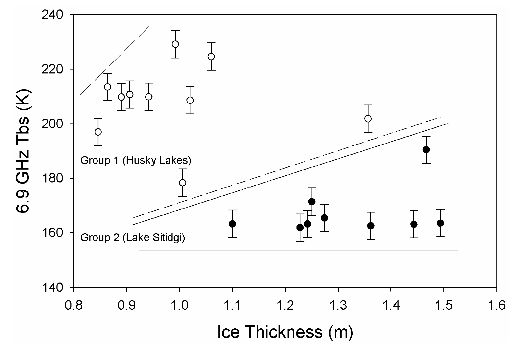
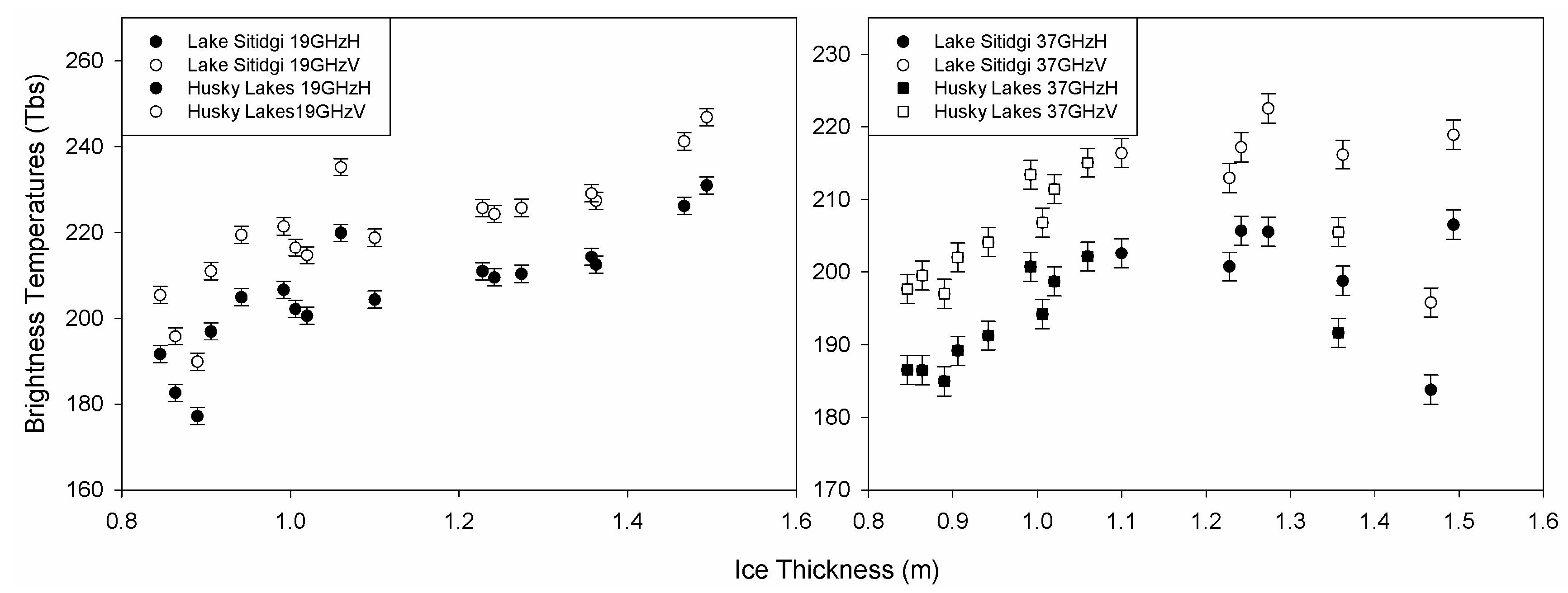
Over lake ice, 37 GHz frequency emission has been successfully simulated over thick ice as the source of the emission emanates from within the ice column (for ice cover thicker than the penetration depth at 37 GHz, 0.75 m). Conversely, simulations for lower frequency emission (6.9 GHz) lack variability noticed in high- resolution airborne and ground-based PM measurements [19]. Freshwater ice thickness studies have identified a direct correlation between ice thickness and low frequency Tb (6.9–19 GHz) [20,21,22,23,24]. In particular, [23,24] demonstrate AMSR-E 19 GHz V sensitivity to ice thickness, noting lower 
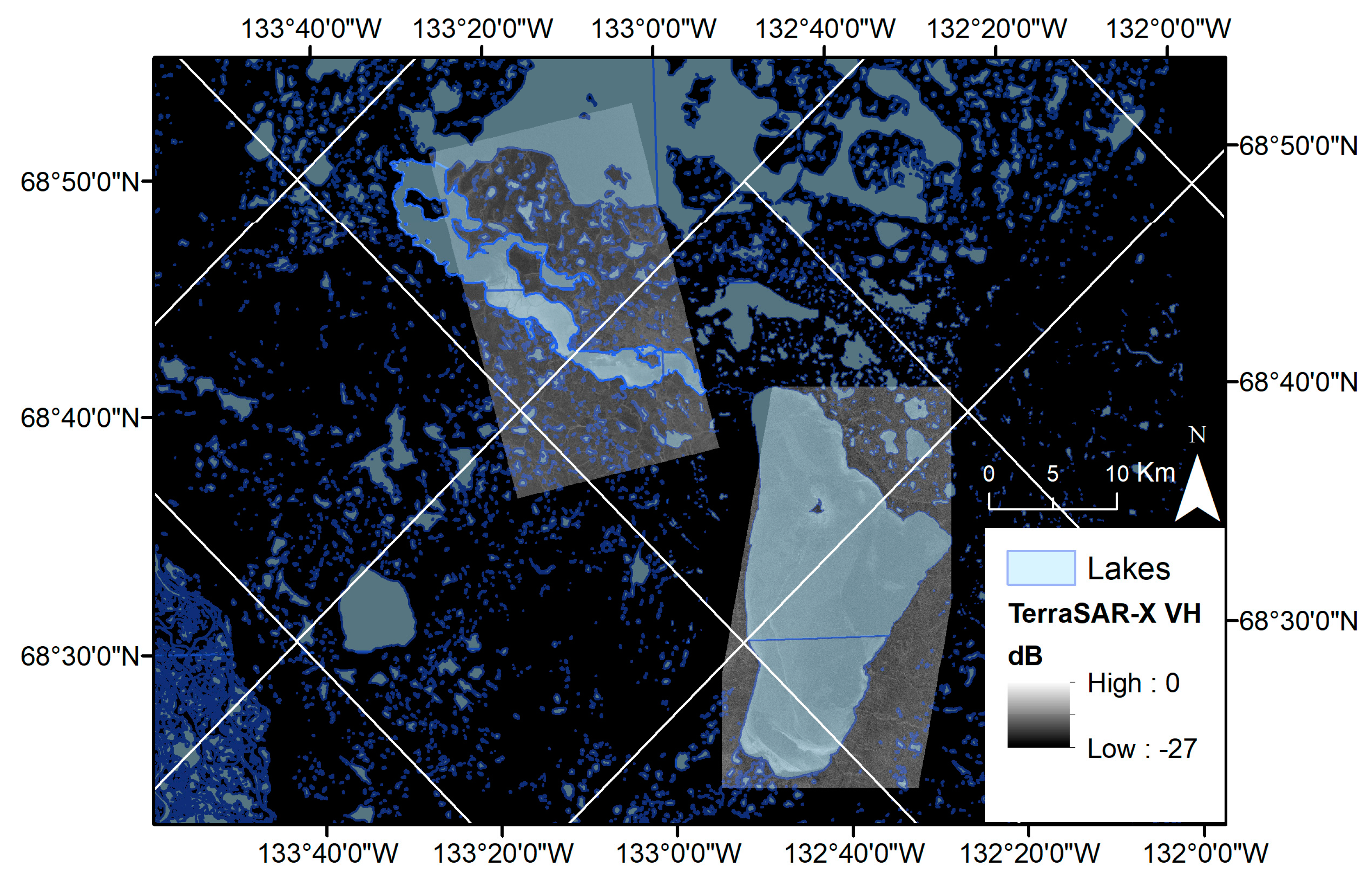
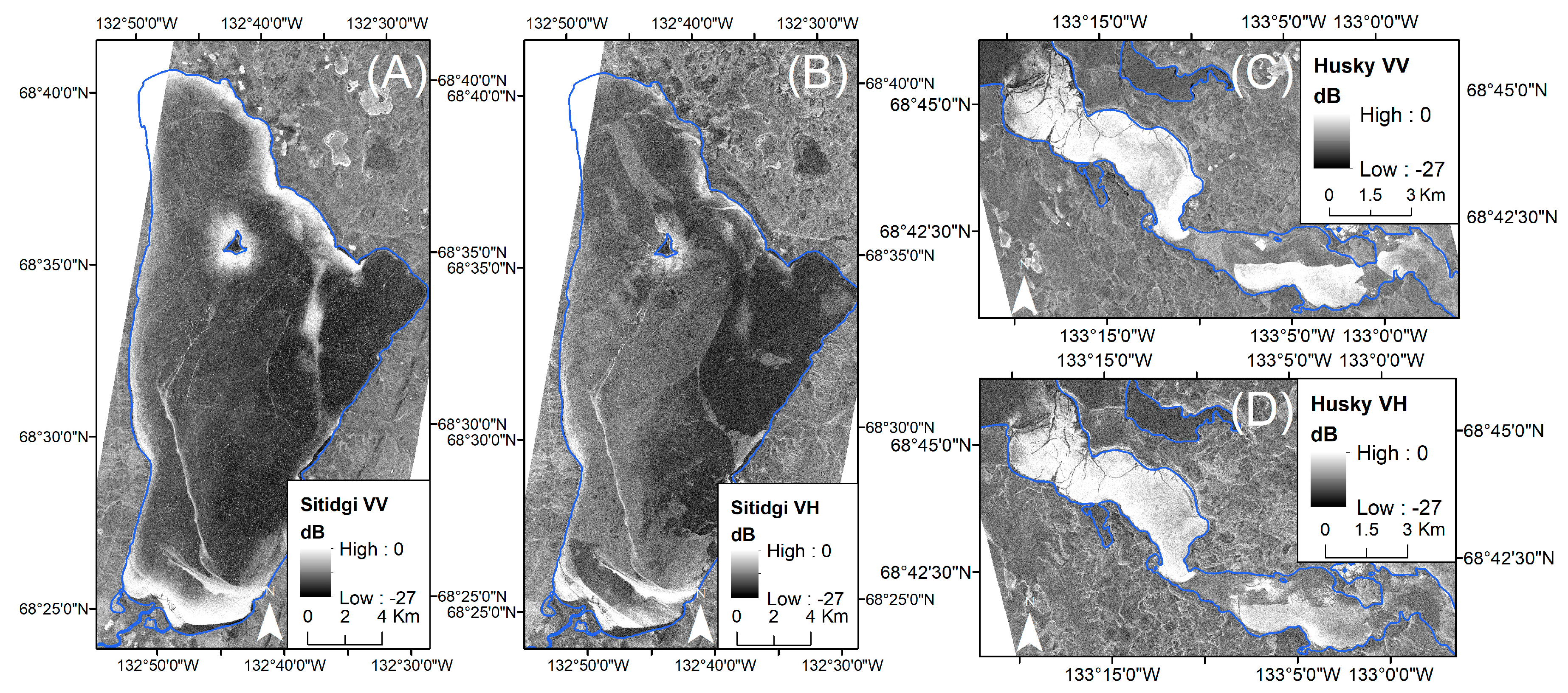
R2 for H-pol due to the potential effect of surface ice types on emission, which includes tertiary ice development (i.e., snow ice, grey ice). Surface ice types, which are typified by the incorporation of variable densities of microbubbles in the surface layers form through (a) snow falling on cooled open water and the freezing of resulting slush, or (b) flooding events caused by pressure cracks or the weight of snow pushing the ice below the hydrostatic water level. In this context, “grey ice” is referring to the incorporation of microbubbles in the surface ice type layers that are not the result of secondary ice development from snow slushing events; not to be conflated with the “grey ice” term used in sea ice studies. Further quantification of emission properties for lakes is restricted by the large spatial footprint of spaceborne PM acquisitions (on the order of tens of kilometers), which often cannot resolve small tundra lakes, illustrated in Figure 1 [21,25,26]. The use of active microwave technology is required to obtain high-resolution measurements to achieve a priori lake-ice information.
Synthetic aperture radar (SAR) backscatter measurements possess a much higher spatial resolution compared to spaceborne PM Tb on the order of tens of meters compared to tens of kilometers, and has been demonstrated to interact with sub-nivean ice properties [20,27,28]. The low dielectric contrast of snow and ice permit transmission of incident microwave radiation through the snow–ice interface at these and longer wavelengths for sub-zero temperature snow with minimal free moisture content. Incident low-frequency microwaves reflect off the ice–water interface if the surface roughness is appreciably smooth with respect to the incident wavelengths due to the large dielectric contrast between media (є′~3 for ice/є′~80 for water), producing low backscatter for clear ice with an inclusion-free column. SAR has been used to classify lakes that have frozen to bottom, as transmitted microwaves interacting with lower dielectric-contrast soil medium produce backscatter similar to terrestrial sites [29,30,31]. If present, any of the following features of freshwater ice can contribute to signal scatter: air bubbles (columnar or spherical in the surface or within the ice volume), deformation features (cracks, rafts), and sediment inclusions [29,30]). In particular, surface ice types (grey, snow ice) have been identified as a source of depolarizing signal interaction [32,33].
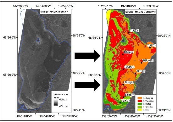
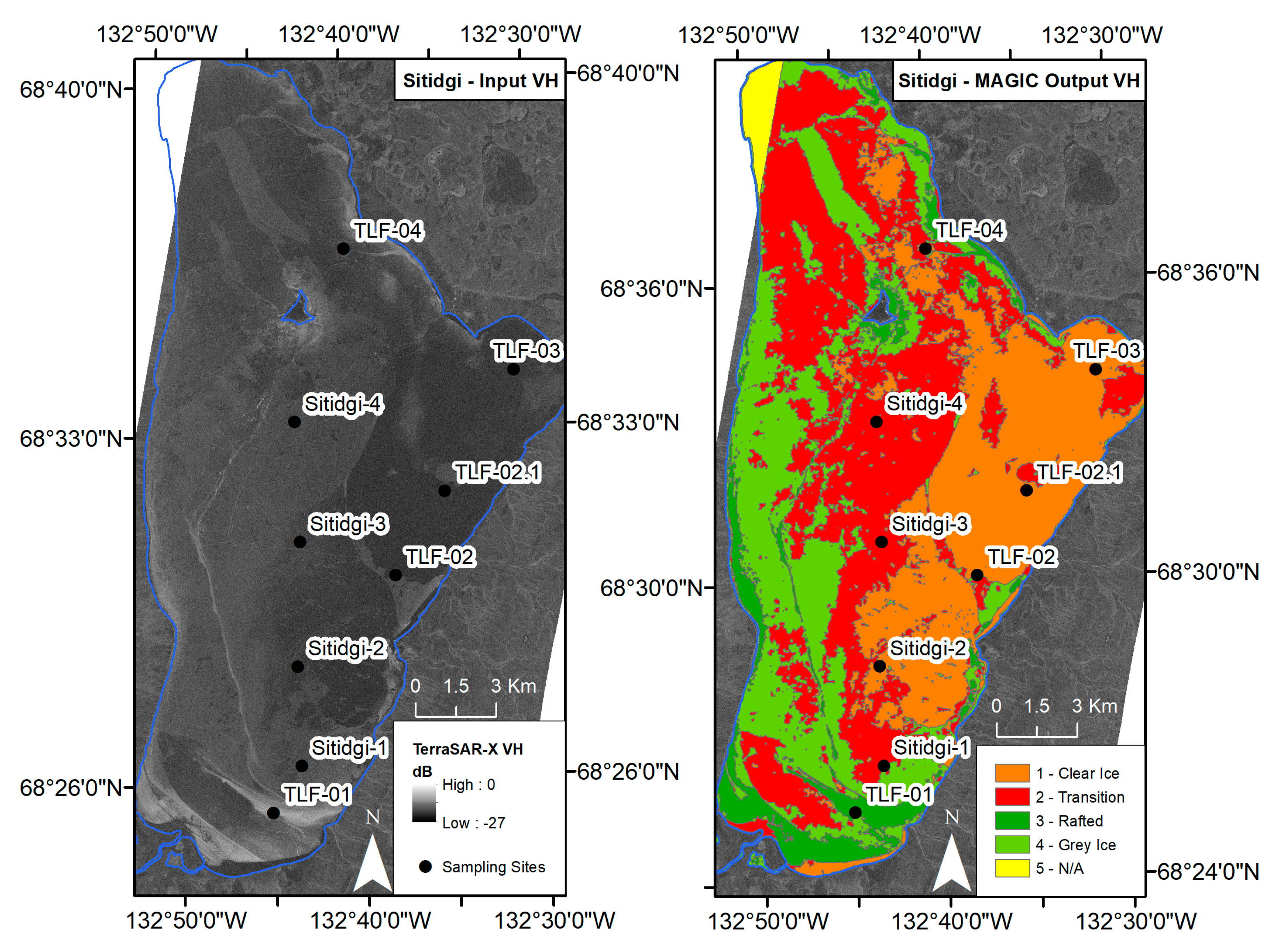
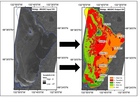
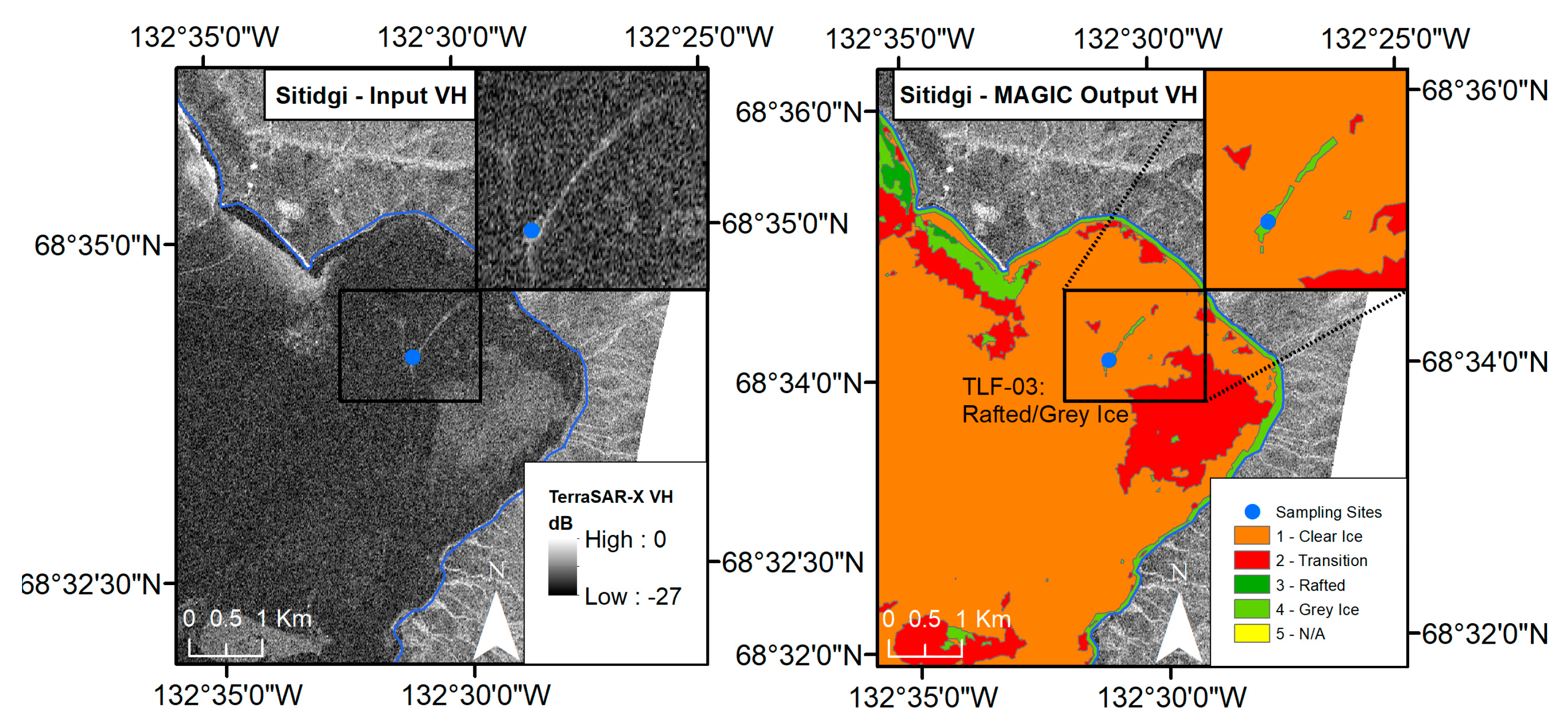
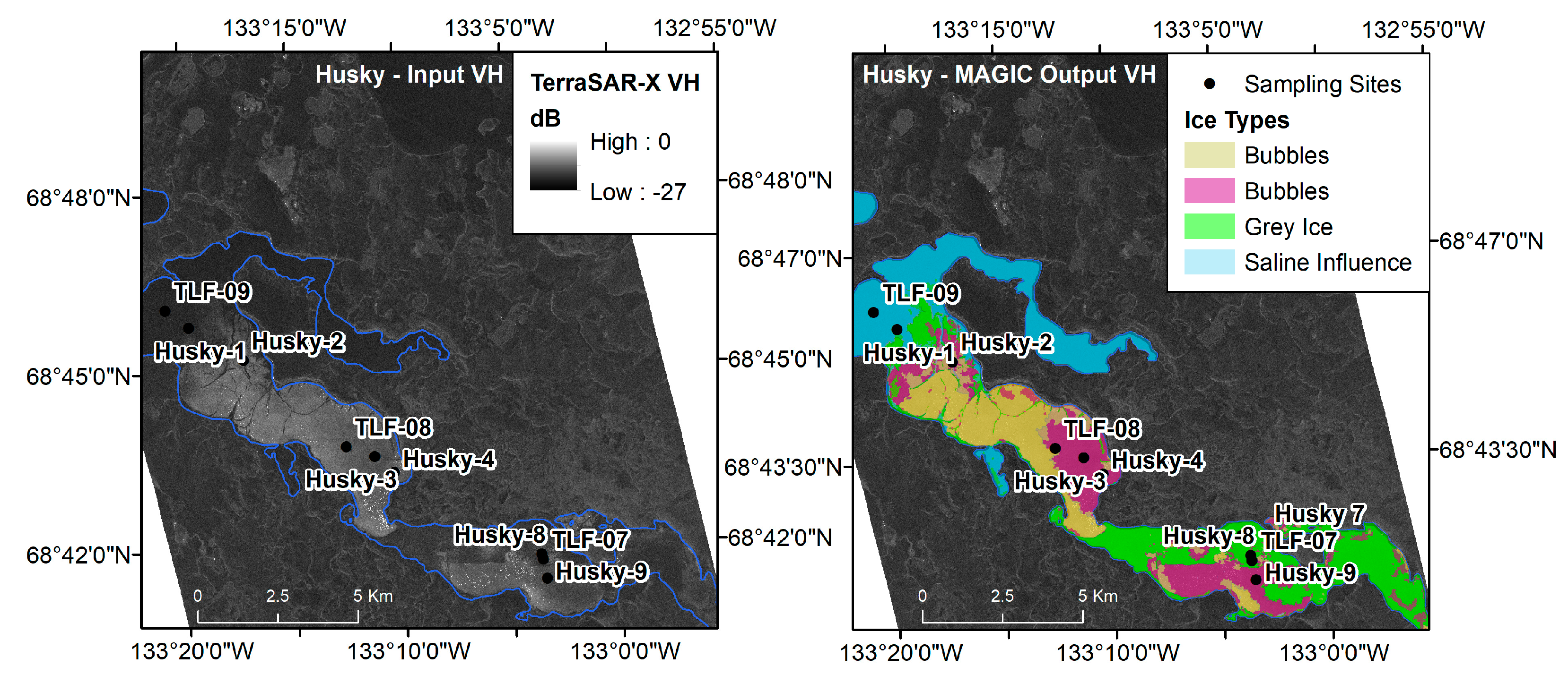
To improve our understanding of passive microwave frequencies utilized in SWE retrieval algorithms in lake-rich environments, a pretext must be produced that identifies the similarities and potential synergy in signal interaction with respect to the presence/absence of surface ice types (snow, grey ice) and SAR observations. With its high spatial resolution, SAR-derived lake-ice information has the potential to complement the assessment of the effect of variable lake-ice types on microwave interaction and overall PM emission. This study presents the effects of differential surface ice types on microwave emission by comparing the behavior of high-resolution airborne PM T
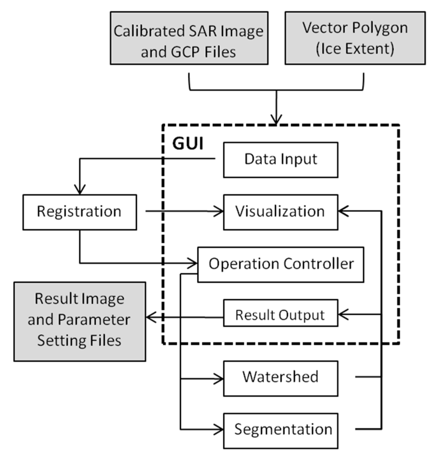
b to spaceborne X-band SAR backscatter measurements. In this study, ice types are delineated by the segmentation software MAGIC (MAp Guided Ice Classification system), described in Section 3 and more extensively in [34]. 
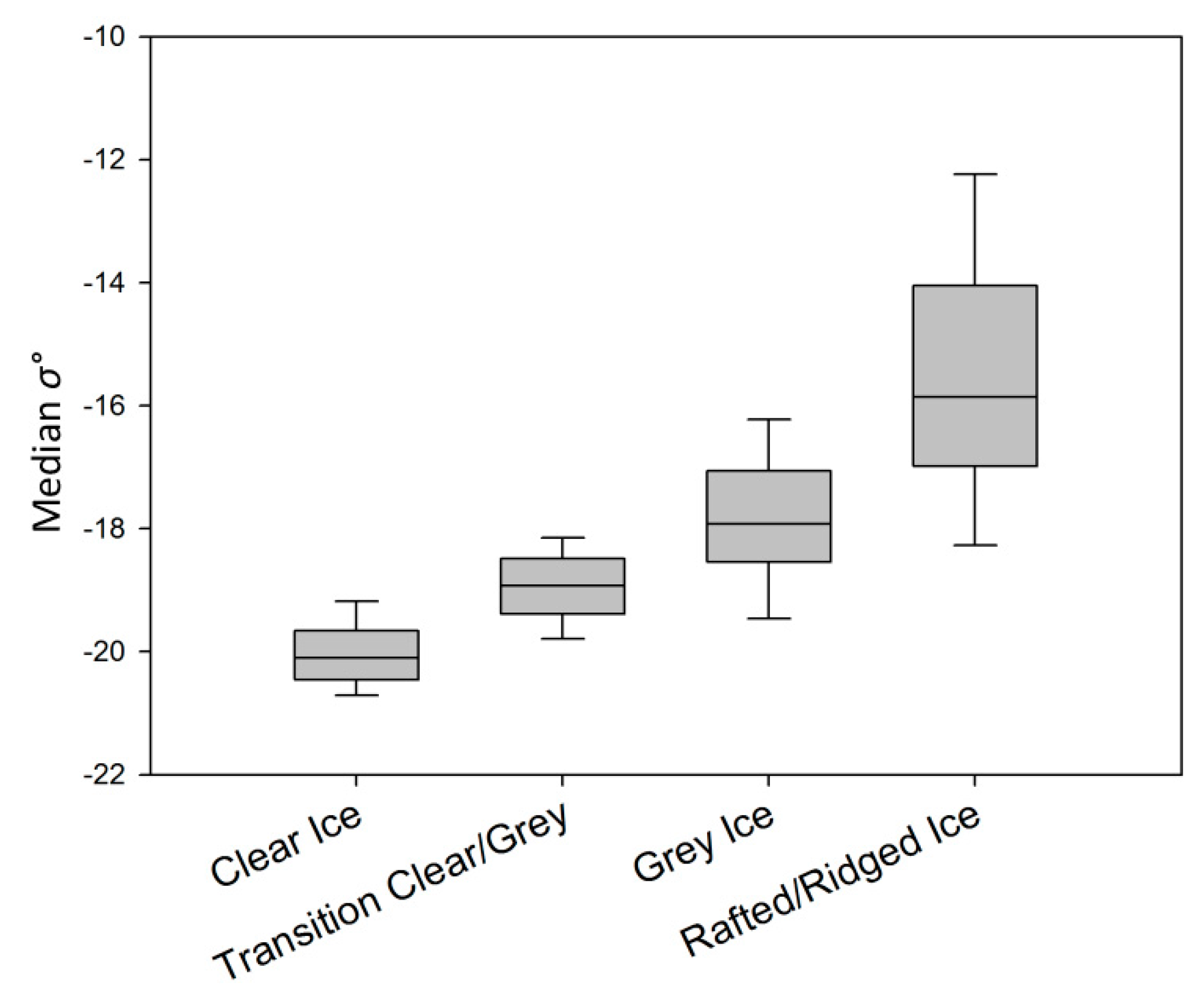
Section 4 presents the use of cross-polarized (VH) MAGIC segmentation classes for the discrimination of surface ice types, and the identification of volume and dihedral scatter using co-polarized (VV) MAGIC segmentation classes. The added ice property information provided by SAR imagery shows the potential to be incorporated into tundra-specific SWE and ice-thickness retrieval algorithms as a priori information to account for the influence of both surface ice types and bubble inclusions on low-frequency (6.9–19 GHz) Tb, described in Section 5.

2. Study Area

Airborne PM and in situ snow and ice observations were acquired in April 2008 over two major lake systems (Sitidgi Lake and Husky Lakes) adjacent to the Mackenzie River delta, approximately 45 km north-east of Inuvik, Northwest Territories (NWT) (Figure 2). The land surrounding the lakes is classified as tundra, sparsely vegetated, and is located in the general boreal forest/shrub transition zone [35]. Climate normals for 1971–2000 retrieved from the National Climate Data and Information Archive http://www.climate.weatheroffice.ec.gc.ca, reported by the Inuvik weather station at Mike Zubko Airport (68.3042° N, 133.4828° W) (Figure 3) describe the area with sub-zero average monthly air temperatures from October to May, sufficient for lake-ice formation. The southern portion of Husky Lakes exhibit low salinity concentrations ranging from 1 to 2 parts per thousand as a result of backflow from the Arctic Ocean through Liverpool bay, while Sitidgi Lake is classified as fresh water [36]. According to bathymetry observations provided by the Department of Fisheries and Oceans (DFO), the average depth of Husky and Sitidgi lakes are 27.8 m and 6.75 m, respectively.

3. Data and Methods

3.1. Snow and Ice Cover Data

In situ snow and ice measurements were collected at a total of nine sampling sites on Sitidgi Lake and 10 sites on Husky Lakes during the period of 6–12 April 2008 (Figure 2). At each sampling site, a total of five surface ice type and thickness measurements were made by drilling an auger hole at a central point, and four others at a distance of 5 m in cardinal coordinate directions in a ‘cross’ pattern. If present, surface ice types constituting the upper layer of the ice volume observed through the auger hole were classified as either clear, clear with bubbles, grey, white, or rough/rafted, with thicknesses of both the full ice cover and surface ice type measured with an avalanche probe with centimeter gradation. Areas with two or more ice types within the sample of 5 auger holes were classified as “variable”. Snowpack measurements consisting of snow depth, density, SWE, grain size and stratigraphy were conducted at each central point, with 30 extra snow depth measurements collected at random throughout the sampling site within 10 m of the central point. Table 1 presents the measured snow depth, SWE, ice thickness and surface ice types observed for each sampling site used in the analysis. Snow depths were collected using a SnowHydro© Magnaprobe, bulk densities using an ESC-30 SWE core tube, and SWE was computed from depth and density measurements.
Summaries of in situ measurements of snow and ice properties at each site are provided in Table 1. Snow stratigraphy in both groups is consistent with the high slab-to-hoar and depth hoar fractions typified by tundra snowpack classification described by [37]. Both brackish and freshwater groups exhibit the same sub-site ice type characteristics, with approximately 31% of sampling sites comprised of one ice type, 56% of sites with two ice types, and 12% with 3 or more. Unique microwave interaction characteristics are expected at Site TLF-01, at the southern portion of Sitidgi Lake where the thick ice combined with the presence of rough and rafted surface ice types present both high emission and scatter potential. Additionally, the low air temperatures observed allow for the assumption that the snowpack remained free from melt and free moisture during the in situ observation period.

3.2. Airborne Radiometer Data

Airborne passive microwave measurements were acquired using Environment Canada’s radiometer system, acquiring Tb at 6.9 GHz, 19 GHz and 37 GHz on 8 April (16:00 UTC, 10:00 local) and 15 April (16:30 UTC, 10:30 local) for Husky and Sitidgi Lakes, respectively, comprised of side-looking dual polarized radiometers (H/V) mounted on board the National Research Council of Canada’s Twin Otter aircraft (See Table 1 of [38] for a full sensor description). PM Tb were collected at an altitude of 279 m and a fixed incidence angle similar to spaceborne radiometers (53°), producing an approximate footprint of 80 × 100 m. Calibration of the radiometers occurred pre and post flights using cold (liquid nitrogen) and warm (ambient temperature microwave absorber) targets. In total, 21 calibrations were performed during the campaign. The calibration procedure aids in providing an approximation of receiver drift experienced during flight. In this dataset, the receiver drift is estimated to be ±2 K at 19 GHz and 37 GHz. The 6.9 GHz channel receiver drift is higher (±5 K for 6.9 H and ±10 K for 6.9 V) as a result of intermittent frequency interference due to radio communication at the Inuvik airport, and a reduced gain between the cold and warm calibration targets. Airborne Tb were collected in transects over Sitidgi Lake, and in clover patterns on Husky Lakes where designated survey sites had not yet been sampled. The aircraft’s position data was provided by the on -board NovAtel-20 GPS system, with an expected vertical/horizontal accuracy of 5 to 10 m because it was not operated in differential mode with an accompanying ground station.
The bearing of each PM Tb was calculated based on the geographic coordinates of the subsequent footprint in each transect, providing the true approximation of the elliptical footprint, as described in [38]. Airborne radiometer acquisitions were collected by selecting the closest Tb footprint to each sampling site to provide 1-to-1 analysis, so long as the site was within 100 m of the footprint. Any sampling site outside the 100 m threshold was used as ancillary data, but not in any Tb analysis. Two transects were extracted for both Husky (~6 and 15 km in length) and Sitidgi lakes (~10 and 29 km in length) in line with in situ transects to illustrate Tb variability over lakes, and to quantify relationships present within the passive and active microwave measurements.

3.3. Spaceborne Active Microwave Data

Spaceborne X-band (9.6 GHz) active microwave SAR observations consisting of two dual-polarized TerraSAR-X (VV, VH) scenes were acquired on 6 April (20:17 local) and 27 April (11:23 local), 2008 for Husky and Sitidgi lakes, respectively. The scenes were both acquired in Stripmap mode with an incidence angle range of 40–43°, meaning that returned signal variability are likely indicative of interactions likely to occur in the media volume as opposed to sole surface interactions. The images were calibrated to sigma nought decibels (σ0 dB) using the Sentinel Application Platform (SNAP) with Terrain Correction performed with a flat-Earth assumption. Both images were multi-looked using a 7 × 7 window, resulting in a spatial resolution of 10 × 10 m (Figure 4). The images were further geolocated using optical SPOT imagery acquired during the summer as a reference image to sub-pixel precision. The median of all TerraSAR-X pixels within the 80 × 100 m bearing-adjusted radiometer footprint (n = 80) was extracted for direct comparison with radiometer observations using the Zonal Statistics tool in ArcGIS. The Noise Equivalent Sigma Zero (NESZ) for Stripmap mode is typically −22 dB. Assuming inclusion-free freshwater ice cover, the penetration depth of incident microwaves was 10 m at 10 GHz [39]. With a maximum observed ice thickness of approximately 1.5 m, incident X-band microwave radiation would interact with the ice–snow and ice–water interfaces, as well as inclusions within the ice (bubbles) and snow (grains) volumes.
The TerraSAR-X images were segmented to provide a coherent grouping of ice classes derived from SAR images. The resultant classes were compared to PM Tb to identify if synergies existing between SAR and PM Tb patterns. To prepare for the MAGIC segmentation algorithm, a consistent linear stretch with custom high and low breaks was applied to each TerraSAR-X acquisition to ensure that all potential values in both the VV and VH bands would be accounted for after conversion to 8-bit imagery (0 dB to −30 dB).

3.4. Model Description: MAGIC

Segmentation of SAR imagery is achieved using MAGIC, which was developed to interpret and segment digital imagery, specifically SAR observations [34]. Segmentation can be completed on full images, but a unique feature of MAGIC is that it is designed to execute segmentation within geocoded polygons overlaid on specific areas of interest. MAGIC provides automated operational interpretation of SAR imagery at a per-pixel basis and can provide a more accurate estimation of ice concentration. Users can also specify the desired number of output classes and draw custom polygons, allowing for independent interpretation of any digital image. Instead of mapping ice concentration, MAGIC is used to identify spatially coherent patterns within backscatter to group like regions into classes that are representative of regions with similar microwave interactions.
The main input files to MAGIC are 32-bit TerraSAR-X (VV, VH) images re-scaled to 8-bit grey scale images stored in BIL (band interleaved by line) format. Other required inputs include polygons detailing the extent of the desired segmentation, and ground control points (GCPs). Segmentation results are stored in BIL or .bmp formats. Figure 5 provides a schematic overview of MAGIC processing steps [34].
The first process applied to SAR imagery is the Watershed algorithm [40], which over-segments the image into several small regions, effectively reducing computational demands of the subsequent segmentation considerably. There are five segmentation methods available within MAGIC: the K-means, Gaussian mixture model, constant multi-level logistical model (MLL), variable MLL, graduated increased edge penalty and the iterative region growing with semantics (IRGS) [34]. Of these methods, the state-of-the-art approach is the IRGS, which is utilized in this analysis.
The IRGS algorithm contains two important components: (1) the use of successive edge penalty functions to produce a traditional Markov random field (MRF) context model to form objective functions, and (2) the solution of the objective functions produced in Equation (3) using a region growing method. Within the IRGS, the MRF can be described using irregular graphs rather than the traditional image lattice. Thus, segmentation is possible for groups of pixels with the MRF context model derived from a regional adjacency graph (RAG). The RAG structure is produced from a purposely over-segmented image constructed by the Watershed algorithm, [41,42] (Figure 5).
The IRGS is iterative; the goal of each iteration is to find the local minimum of an objective function [42]. The number of classes within the over-segmented image is reduced to the theorized number of “true” classes. In locations that classes are paired, if the energy ( δ E i j ) of merging two nodes is reduced compared to the energy before merging, the merging is justified by Equation (3). The difference in energy for two neighboring regions R i and R j and its union R k = R i R j is provided by
δ E i j = s R k ln ( σ k ) s R i ln ( σ i ) s R j ln ( σ j ) β s , t C s R i , t R j g ( s t )
where s R i , j , k represent a series of discrete valued random variables that constitute regions ( R ) with specific nodes i , j , k . σ i , j , k are Gaussian parameters for each class, β is the MLL model parameter, and s ,   t C is the set of all cliques on the lattice (image grid) S . [42]. g ( s t ) represents the penalty function which defines the speed at which the edge penalty decays with increased edge strength [42].
If Equation (3) produces a negative number, R i and R j are able to merge; if Equation (3) produces any non-negative number, R i and R j are not merged. In Equation (3), energy differences are only calculated for nodes within the same class, restricting region growth to those classes. This is designed to prevent the merging between classes for objects that exhibit weak boundaries, referred to as semantic region growing [43]. A more detailed description and derivation of the IRGS algorithm is available in [41,42].
The IRGS algorithm was applied within MAGIC to perform a segmentation of 8-bit greyscale VV and VH TerraSAR-X images over Husky and Sitidgi Lakes. GCP points were extracted from the input imagery, and a text file of polygon nodes delineates lake extent. A total of five ice classes for Husky and Sitidgi Lakes were selected for analysis, determined from the amount of ice types observed within the in situ measurements.

4. Results

4.1. Brackish/Freshwater Class Delineation From Passive Microwave Tb

Lower frequency Tb (6.9 GHz, 19 GHz) are expected to correlate positively to lake-ice thickness measurements, as continued lake-ice growth results in less radiometrically cold water included in the overall microwave emission [21,23,26]. Concurrently, when viewing all in situ ice thicknesses relative to 6.9 GHz Tb, the emitted signal exhibits a negative association. However, there are noticeable groupings within the 6.9 GHz Tb (Figure 6). The groups are spatially coherent, with measurements in Group 1 located in the Husky Lakes and those in Group 2 located in Sitidgi Lake. Data provided by the Department of Fisheries and Oceans (DFO) indicate that backflow of saline water from the Arctic Ocean infiltrates through Liverpool Bay up to a concentration of 20 parts per thousand (ppt) in the summer months, reducing in concentration to 1–2 ppt in the southern portion of Husky Lakes and diminishing at the inflow of the river connecting Sitidgi with Husky lakes [36]. The presence of brine inclusions enhances the emissivity of the ice medium, thereby raising Tb for Group 1, consistent with [37]. The following analysis splits the in situ observations into brackish (Group 1) and freshwater (Group 2) division, comprised of sites with similar physical and emissive properties.
For frequencies higher than 6.9 GHz (19, 37 GHz), the microwave emission of floating ice is theorized to be influenced in large part by ice thickness and ice types [26]. The distribution of Tb for 19 GHz and 37 GHz over the range of ice thicknesses observed in both Husky (brackish) and Sitidgi (freshwater) lakes is provided in Figure 7. In Husky Lakes, the majority of ice thickness measurements range from 0.85 m to 1.06 m, approaching the upper limit of the one-way penetration depth at 37 GHz (0.7 m, calculated by [14]), resulting in a steady increase of emission for thicker ice. Similarly, the one-way penetration depth of 19 GHz (at 230 K) is approximately 4.2 m, indicating that radiometrically cold water is incorporated into signal emission at all sites.
The influence of ice thickness on observed Tb for 19 GHz and 37 GHz is presented in Figure 5. 19 GHz Tb increase relative to increases in ice thickness. At all sites in this study, ice is much thinner than the penetration depth of 19 GHz, meaning that it is likely that the influence of radiometrically cold water is reduced as ice thickness increases, but the depth of emission will always be lower than the ice–water interface. At 37 GHz, Tb at both polarizations increase up to a lake-ice thickness of about 1.1 m, after which Tb remain at about the same level or start to decrease again towards larger thickness values. This can possibly be interpreted as the Tb increase up to about 1.1 m represents the fading influence of the water underneath the lake ice with increasing thickness. It is noted that the theoretical limit of the penetration depth at this frequency would be 0.7 m [14]. Therefore, 37 GHz Tb for sites with ice thickness greater than this limit is independent of the influence of radiometrically cold water (Figure 7). The source of emission is still within the ice cover and is potentially affected by variable ice conditions such as surface ice types and roughness. For example, Site TLF-01 has an observed ice thickness of 1.47 m and is situated in a region of rough, rafted ice, which exhibits increased surface ice types that scatter 37 GHz Tb, lowering observed Tb by approximately 20 K (Figure 7). The site TLF-01 also increases 6.9 GHz H Tb by approximately 30 K, indicating that the physical properties of the horizontal structuring of rafts and rough ice allow for increased Tb.
As referenced previously, classic SWE retrieval algorithms developed for the hemispheric “Chang” algorithm [10] or open environment applications [9] underestimate SWE as a function of lake-ice fraction and thickness: the larger the lake-ice fraction and the thinner the lake ice within the sensors' footprint, the larger the decrease of TB at 19 GHz due to microwave emission from water below the ice. SWE retrieval using these traditional algorithms is consistently below measured levels, with extremely low root mean square error (RMSE) and negative mean bias error (MBE) (Table 2). Sites that overestimate in situ SWE correspond to sites with thick ice (>1.05 m) in Husky Lake, or sites that exhibit surface ice types (grey, rafted ice) in Sitidgi Lake. Tb departures caused by surface-ice types remain a key consideration in the improvement of SWE algorithms; the ability to provide segmentation of which is explored using MAGIC in the following section.

4.2. MAGIC Segmentation—Sitidgi Lake

Ice formation patterns in the winter of 2007/2008 produced variable surface-ice type development over Sitidgi Lake, while there are largely no surface-ice types present at Husky Lakes other than clear ice. Therefore, image segmentation and active/passive microwave observations over Sitidgi Lake exhibit variability based on surface and volume scatter considerations, whereas for Husky Lakes it is likely backscatter/Tb variability caused by volume scatter and salinity considerations.
Previous PM lake-ice studies notice Tb variability in the presence of surface-ice types [44,45], but these have not been quantified with coincident co- or cross-polarized SAR backscatter. Thus, the investigation of surface-ice type classification and delineation through the comparison of SAR and PM Tb is of interest for ice-type mapping. Figure 8 shows surface ice-type segmentation derived using MAGIC from cross-polarised (VH) TerraSAR-X observations of Sitidgi Lake. High cross-polarized backscatter (VH) values correspond to grey and rafted ice according to our in situ measurements (see Table 1), which exhibit greater potential for depolarization of the SAR signal. Conversely, we find that sites with clear ice (see Table 1 and Figure 2) correspond to low VH backscatter values at X-Band. Variability in cross-polarized (VH) σ0 is determined to best represent ice types based on the in situ measurements; an increase in backscatter corresponds to an in situ measurement exhibiting greater potential for depolarizing scatter events (grey and rafted ice), whereas areas of low VH σ0 correspond to clear ice. Based on in situ observations co-located with the SAR images of Sitidgi Lake, unique backscatter values can be assigned to each of the following four surface-ice types: clear ice, a transition zone between clear and grey ice, grey ice, and rafted ice (Figure 8).
High VV backscatter values are either observed in areas of rafted ice (TLF-01 in Figure 8) or in areas with a large bubble concentration at the ice underside due to tubular bubble development [27,31]. The spatial distribution of high VV backscatter observations indeed suggests that these are caused by a bubble-rich ice underside (Figure 4). Most high-backscatter regions at the VV polarization are located in shallow areas close to shore or the island in the centre of the lake, where tubular bubble formation at the base or bottom of the ice volume is most likely to occur [31].
Mann–Whitney test (U-stat) statistics were calculated to determine the probability that the difference in distribution of the two samples would be greater than expected by chance, and therefore would not be from the same population. A p-value of 0.00 at a significance level of 0.05 denotes that the null hypothesis (sample 1 = sample 2) is broken, and the samples are statistically unlikely to be from the same population. The test is applied to the distribution of σ0 pixels contained within the airborne PM Tb footprints that coincide with sampling sites, with results shown in Table 3.
The clear-ice group (orange in Table 3 and Figure 8) exhibit p-values greater than 0.01, indicating that the σ0 values extracted from the PM footprint are statistically likely to be sampled from the same population. Other groups generally exhibit non-significant p-values observed when within the same group (i.e., TLF02.1, TLF02, Sitigi-2—see Table 3 and Figure 8 for color-coding). Significant p-values are observed when comparing sites between ice-class types (clear vs transition, or clear vs rough/rafted ice). Within the transitional ice class, several sites exhibit statistically different distributions, discrepancies that are potentially explained by the situation of the sampling sites within MAGIC-derived ice classes. Sites within the “transitional ice types” class are situated on boundaries of MAGIC-defined ice-type zones (Figure 8). The method used to classify ice types within MAGIC was the IRGS, where classification is based on the growth of like-valued regions. Therefore, sites at the boundary zones between these regions may have values that are less similar to the complete distribution of that class, resulting in non-significant p-values.
The distributions of all σ0 values for each ice type was also tested using a t-test, with boxplot distributions of backscatter for each class displayed in Figure 9. Each ice class produced p = 0.00 (at a significance of 0.05), indicating that the sample of σ0 values for the ice classes are not likely sampled from the same population.
Figure 10 shows MAGIC segmentation output for the north-east quadrant of Sitidgi Lake. Two sampling sites (TLF-03 and TLF-02.1) are present within the subset to be used as ground-truth data. Consistent with Figure 8, high VH backscatter areas are coincident with grey and rafted ice classification, and areas of low VH backscatter classified as clear ice. There is potential for speckle caused by constructive and destructive coherence within the clear-ice class to produce values consistent with the transitional clear/grey ice class. However, the region growing aspect of the IRGS algorithm [32] ensures that outliers are captured within like groups, while markedly different backscatter caused by variable ice types at TLF-03 in Figure 10 are segmented correctly. Surface-ice type classes are observed to be both spatially (Figure 8) and statistically significant (Table 3) using the MAGIC IRGS segmentation algorithm.

4.3. MAGIC Segmentation—Husky Lakes

In contrast to ice surface conditions observed on Sitidgi Lake, the ice on Husky Lakes is predominantly composed of clear ice (see Table 1), with the exception of two sampling sites (Husky 8 and TLF-07. The spatial distribution of sigma nought values in Husky Lake is similar for VH and VV-polarization—specifically zones of high backscatter in the central and south half of the southern basin (Figure 4). This indicates that the scattering mechanisms causing high σ0 in the co-polarized image are also sufficient to depolarise incident microwaves. Consistently high backscatter in both the VV and VH observations also indicate that even if grey ice is present at the surface in Husky Lakes, the majority of power returned would be caused by the interaction at or near the ice–water interface [46,47]. Therefore, if surface-ice types and a rough interface caused by tubular bubble development are both present, the σ0 return from the surface will be of much lower magnitude than surface interaction returns from the ice–water interface. Figure 11 displays the MAGIC VH segmentation and proposed ice-type classification based on interpretation of the image.
An interesting feature within X-band observations of Husky Lakes is potentially caused by the influence of the low-level salinity water caused by infiltration from the Arctic Ocean [34]. The incorporation of low-level salinity within the ice or at the snow–ice interface (as a result of slushing events caused by pressure cracks or from the ice being depressed below the waterline) results in a higher-loss medium similar in physical properties to brackish first-year sea ice. Areas of extremely low backscatter are present in the north-west portion of Husky Lakes in both the VV and VH TerraSAR-X images, indicative of either an inclusion-free ice cover and a smooth ice–water interface, or absorption from a lossy medium [48]. During the campaign neither the water nor salinity concentrations were measured, but were generalized by [49] and measured in subsequent field observations in 2013. In situ salinity measurements in the northern basin in April 2013 collected 3 m below the ice surface revealed salinity levels between 1–3 ppt, classified as “brackish” conditions. The bulk ice salinity decreased from 0.4–0.6 ppt near the surface to 0.2 ppt at greater depths, indicating the presence of brine pockets within the ice. While salinity levels in the northern basin of Husky lakes collected in April 2013 could not be extrapolated back to April 2008, the presence of brine below and within the ice column suggests inclusion of an additional ice type into MAGIC: brackish sea ice. Without contemporaneous absolute salinity measurements, an explicit comparison to backscatter over sea ice cannot be made. Therefore, the likely presence of brine pockets restricts an accurate assessment of ice types in the Husky lakes. However, the unique physical characteristics of the Husky Lakes potentially provide a broader dataset for comparison with PM emission.

5. Active/Passive Microwave Relationships

5.1. Sitidgi Lake—Active/Passive Transects

Single transects have been isolated from the PM dataset over Sitidgi Lake to compare Tb with the TerraSAR-X backscatter observations and corresponding radar returns and the associated lake ice types derived by MAGIC. Figure 12 displays the spatial extent of transects 1 and 2 over Sitidgi Lake, and the sequential Tb/backscatter measurements from start point “A” to end point “B”. 19 GHz H Tb appear to display a relationship with co-located cross-polarized (VH) σ0 values. 19 GHz H Tb also exhibit much more noise than the coincident VH σ0 returns as a result of inherent smoothing within the backscatter measurements, as each σ0 value is the median of 80 pixels within the passive microwave footprint. Positive correlations with the X-band σ0 are also noticed with 19 GHz V, and both 6.9 GHz H and V polarisations (Table 4).
Figure 12 also indicates which MAGIC-derived ice types are spatially coincident to X-band σ0 and 19 GHz H PM Tb. Transect 1 contains classes defined as clear ice, the clear/grey ice transition zone, grey ice near the north end of the transect, and a considerable amount of rafting at the south end. The highest correlation between the X-band σ0 and Tb was observed at 6.9 GHz, regardless of polarization (Table 4). Concurrently, the correlation between Tb at 19 GHz H and V were smaller, but there were positive correlations with co-located median X-band σ0.
Transect 1 also contained a considerable amount of footprints that exhibited interaction at or near the ice–water interface, notably around the island in the northern region of Sitidgi Lake. While footprints with land inclusions were filtered out of the transect, the shallow depths around the island were sufficient to cause the formation of bubbles near the ice–water interface, and an increasing rough interface with respect to the incoming wavelength, producing subsequently high observed σ0.
Transect 2 contains classes defined as clear ice and the clear/grey ice transition zone. 19 GHz H Tb and TerraSAR-X VH σ0 exhibited a moderately strong positive correlation coefficient of 0.63 for Transect 2, however nearly zero correlation at 19 GHz V.
There was a stark contrast between the positive correlation coefficient in 6.9 GHz V/H and 19 GHz V noticed in Transect 1 and the low positive correlation in Transect 2 (Table 4). This contrast may be indicative that 6.9 GHz is sensitive to grey ice, rafted ice or bubble inclusions near the ice–water interface, but not extremely sensitive to changes in ice cover noticed in Transect 2 (clear to transition zone).
Table 5 presents the overall distribution of passive microwave Tb with respect to TSX backscatter values that comprise the segmented groups derived by MAGIC. Overlap exists in the distribution of Tb for all ice groups when observing the upper and lower quartiles, which is caused by the region growing aspect of MAGIC’s IRGS algorithm where outlier values are included into spatially exclusive classes, reducing the amount of small isolated classes in the image. However, median Tb for H-pol frequencies increase together with X-band VH backscatter, identifying that it is possible to establish relative Tb distribution patterns for PM Tb and σ0 returns based on in situ ice types.

5.2. Husky Lakes—Active/Passive Transects

Transects extracted from the PM dataset over Husky lakes exhibit differential Tb and backscatter characteristics compared to Sitidgi Lake, caused by the absence of surface-ice types and the presence of salinity. Areas of high backscatter are coincident with sampling sites that are classified as “clear ice”, and areas of low backscatter (such as the north extent of transect 2 (Figure 13) are coincident with “grey ice” classifications. According to patterns present in VH returns over Sitidgi Lake, this indicates that another physical mechanism is controlling backscatter returns from the Husky Lakes. Table 6 shows negative correlation coefficients when comparing PM Tb to backscatter, and are strongest at 6.9 GHz H/V and 19 GHz V. In Figure 13, 19 GHz V is displayed to illustrate PM Tb characteristics relative to in situ ice properties.
Transect 1 covers the spatial extent from the eastern point of the main Husky Lakes channel to the outlet of larger, more saline lakes and channels that connect to Liverpool Bay. In situ sampling sites coincident to transect 1 are all classified as areas of clear surface ice. High backscatter returns and low PM Tb at those sites are consistent with the presence of interaction at the ice–water interface due to surface roughness caused by tubular bubble inclusions. In the middle of the transect where large cracks are apparent (Figure 13), it is unclear from in situ observations what physical property is controlling the variability in the microwave measurements. For example, the sub-site variability of ice types at Husky-2 (classified as clear ice) contains 3 clear-ice measurements, 1 clear-ice with bubbles at the surface measurement, and 1 grey-ice measurement. The grey-ice sampling site is coincident with low backscatter/high PM Tb areas, and the clear-ice sites are located over areas of high backscatter/low PM Tb (not shown). In the westernmost portion of the transect, it is apparent that salinity concentration in the water is sufficient to be incorporated into the ice or mixing with surface snow as slush during flooding events. The inclusion of brine pockets into the ice have reciprocal effects on emission and backscatter, as it raises the emissivity of the medium, but also increases loss, thereby raising (lowering) emission (backscatter) [43,44,48]. Absolute differences in Transect 1 as a result of brine inclusions generally increase PM Tb by approximately 8 K, while backscatter returns dropped by approximately 4 dB.

6. Discussion

Common 19–37 GHz difference algorithms are confounded by variable Tb in the 19 GHz channel due to the combination of dielectric properties (ice/water) at the emission source [16,26]. Single-frequency algorithms that track the temporal development of the Tb difference between adjacent months show improvement for SWE estimates in tundra environments when the combined snow/ice thickness exceeds the penetration depth [26]. However, high RMSE and mean bias errors still exist, indicating that 37 GHz Tb variability may also be influenced by sub-nivean properties. The quantification of emission properties for surface-ice types or bubbles within ice are not included in current single (37 GHz) or dual (19/37 GHz) frequency-difference SWE algorithms. This study affirms that 19 GHz Tb are affected by ice thickness but indicates that Tb are further affected by surface-ice types and bubble concentration near the ice–water interface. The results presented in this paper present an opportunity to quantify the location and emission properties of ice types based on a priori information from the segmentation of co- and cross-polarized TerraSAR-X acquisitions. Additionally, the quantification of the influence of surface-ice types and bubbles within ice on emission has the potential to improve low frequency Tb simulation, where the ice column has commonly been simulated as pure congelation ice absent of heterogeneities [18,19].
Tb variability caused by ice type or bubble inclusion also presents implications for PM ice-thickness retrieval. Kang et al., [23] exhibit high correlation for ice thickness at 10.7 GHz H and 18.7 GHz V Tb, postulating a direct relationship for increased emission with thicker ice over large freshwater lakes (Great Bear and Great Slave Lake); 18.7 GHz V Tb are reported to obtain higher correlation and lower standard deviation compared to 19 GHz H-pol [23]. The variability of H-pol Tb resulting in lower correlation values with a higher standard deviation implies interaction with surface/horizontally positioned scattering media [50]. Accurate knowledge of ice-type presence and influence on total emission over larger lakes present the potential for improvement of PM 19 GHz ice-retrieval algorithms.
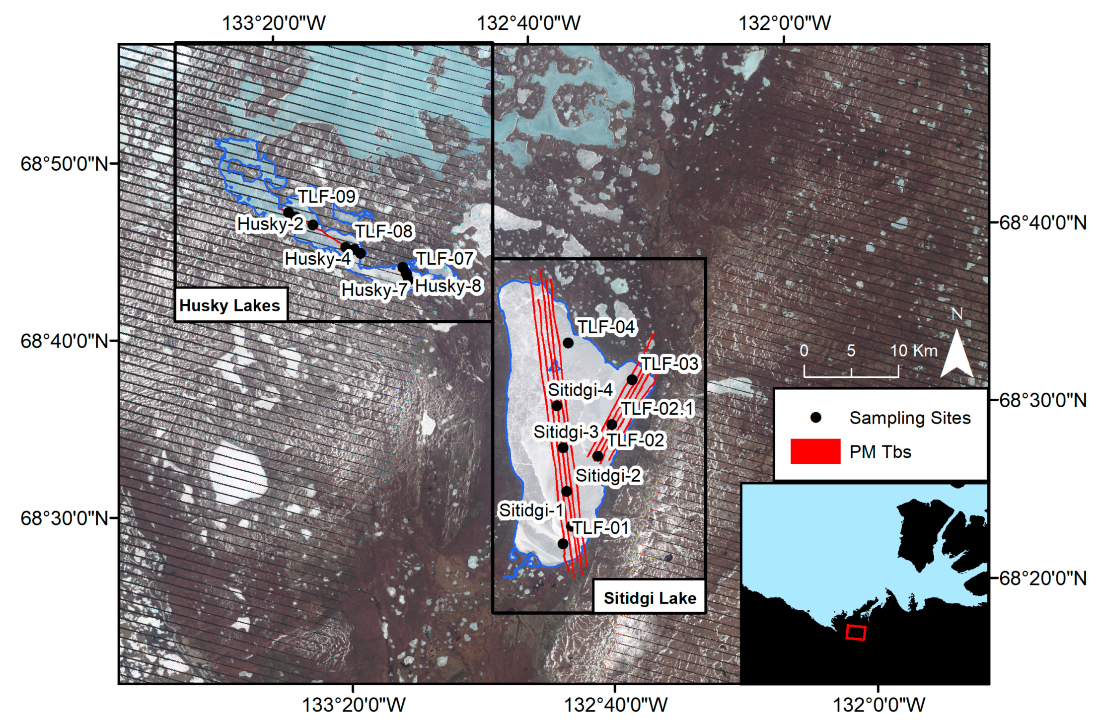
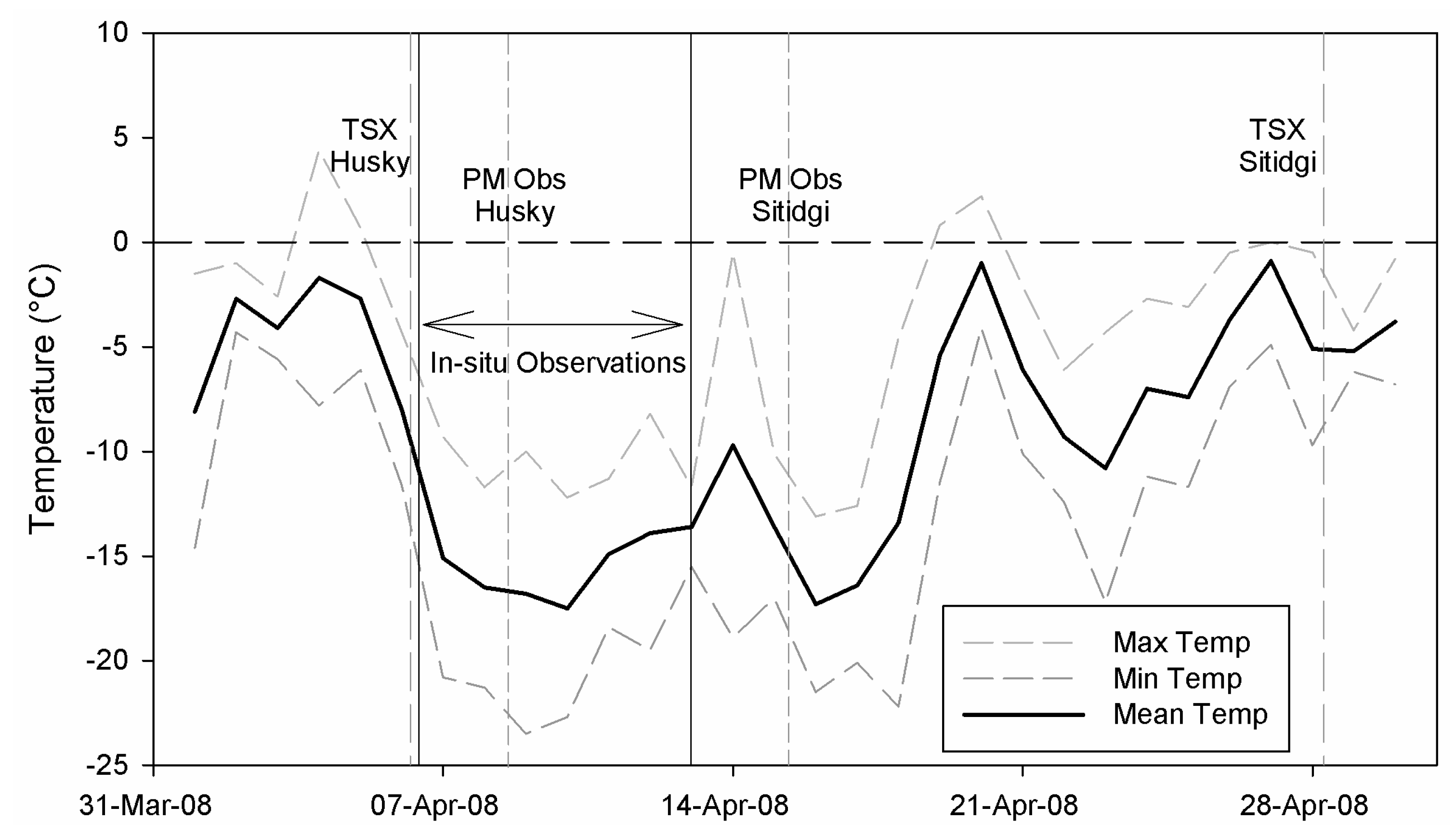
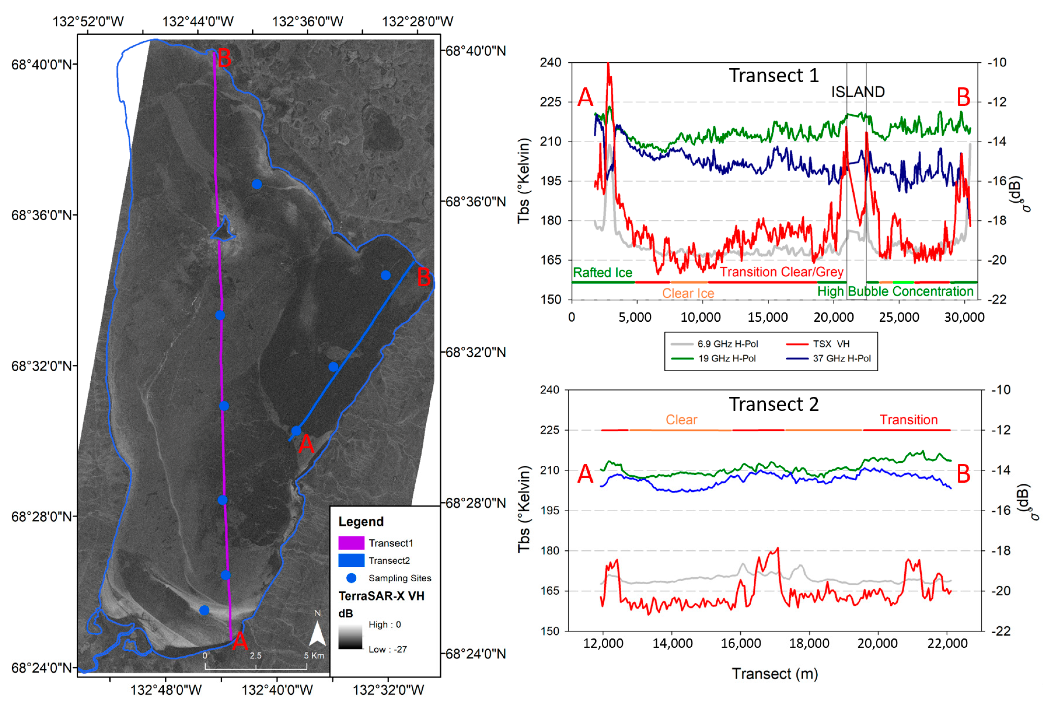
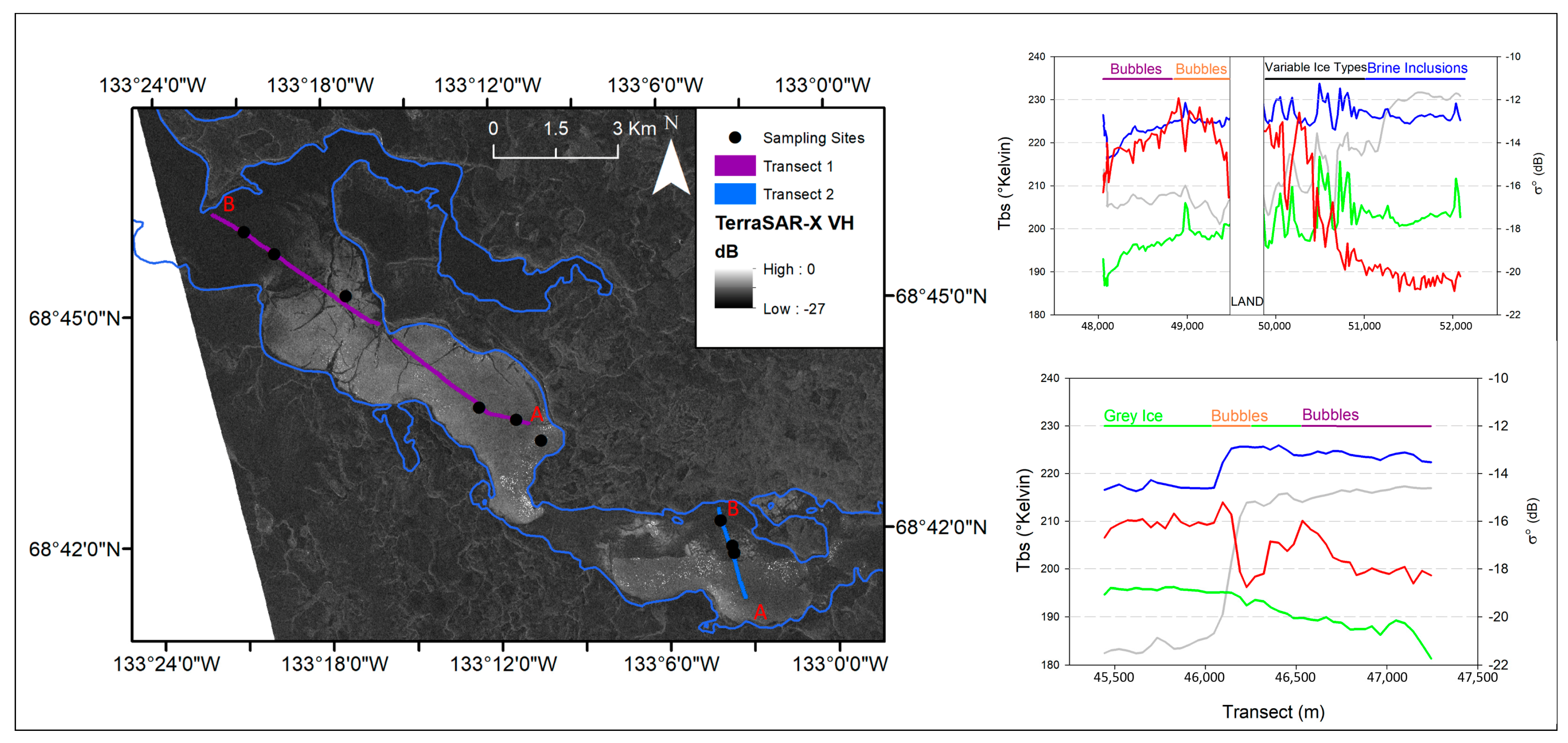
This analysis assumes the consistency of the relation between Tb, σ0, and the physical snow and ice parameters as measured in the field. At Husky Lake, in situ measurements were collected 3 days prior to airborne Tb observations (15 April 2008) and 6 days after the TerraSAR-X acquisition (6 April). At Sitidgi Lake, the measurements were collected 4 days before Tb observation and 19 days prior to TerraSAR-X. The potential exists in this time period for pressure cracks to occur, flood the ice surface and develop surface-ice types, but no free water was observed within the snowpack or at the ice surface during in situ measurements. Weather station data from Mike Zubko airport indicates that the entire study period sustained sub-freezing temperatures, indicating that snow melt is unlikely to influence microwave observations. Future observations in this region are required to advance the hypotheses presented regarding the ice conditions on Sitidgi and Husky lakes, ideally with a denser time series of in situ measurements, passive microwave and SAR data acquisitions.
The influence of surface ice types has not yet been considered as a source of error in SWE-retrieval algorithms because it has been hypothesized generally that the errors are the result of the inclusion of radiometrically-cold water being incorporated into the “background” 19 GHz Tb. This study has identified 19 GHz Tb increases of 20–30 K in regions of severely rafted ice, and 15 K where grey surface-ice types are present. Additionally, cross-pol TerraSAR-X acquisitions are useful in identifying the location of surface-ice types as demonstrated using MAGIC. Further investigation is required into the effect of surface-ice types on lake ice emission, because high-resolution passive microwave observations are not consistently available. With the low resolution of spaceborne PM observations, the use of cross-pol SAR may allow for the supplement of ice-type concentration, accounting for the effect of lake-ice types within passive microwave emission.

7. Conclusions

This study examined the effect of the variable lake ice properties on coincident passive and active microwave measurements over Sitdigi and Husky Lakes. The study assessed the potential of developing the basis for operational a priori lake ice-type information to improve the understanding of microwave interaction with floating lake-ice parameters. Results demonstrate the segmentation program MAGIC can be used to derive ice classes based on like σ0 values within regions, while incorporating the consideration of radar speckle. MAGIC requires in situ measurements pertaining to the amount of lake-ice types present, but does not differentiate between surface and volume scatter. MAGIC outputs for Sitidgi Lake provided spatial consistency for ice types present within the in situ samples. The segmentation derived by MAGIC over Husky Lakes effectively delineated areas of high bubble concentration near the ice–water interface in the absence of surface lake-ice types.
TerraSAR-X (9.6 GHz) measurements over Sitidgi and Husky lakes exhibit contrasting relationships with airborne passive microwave Tb. X-band VH σ0 exhibit highest correlation with 19 GHz H over Sitidgi Lake (Transect 1: R = 0.58, Transect 2: R = 0.56), and 19 GHz V over Husky lake (Transect 1: –0.37, Transect 2: −0.63). The contrasting relationships appear to be the result of the variable physical characteristics of the ice at: (a) the ice–snow interface; (b) the ice–water interface; and (c) the sub-ice mediums (water or lake-bottom). Fluctuations in both backscatter and Tb for Husky Lake are potentially the result of bubble inclusions modifying the surface roughness at the ice–water interface which provides a dominant source of scatter in even the cross-polarized measurements. Increasing salinity concentrations in the north-west Husky Lakes appear to be causing decreases in backscatter and increases in Tb. Further investigation is required to quantify the effect of surface lake-ice types on Tb and σ0 over large lakes such as Great Bear and Great Slave Lake. The large sizes of these lakes size allow for pure lake ice passive microwave observations using satellite sensors, and offer the best potential for the improvement of lake-specific SWE-retrieval algorithms.

Acknowledgments

This research was supported by a Government of Canada IPY grant (Variability and change in the Canadian Cryosphere, Anne Walker, PI) and an NSERC Discovery Grant to C. Duguay. Thanks to Ken Asmus and Walter Strapp (Environment Canada) for support with radiometer measurements and processing, and Arvids Silis and Erin Thompson (Environment Canada) for contributing field measurements. Our thanks is also extended to Professor David Clausi for providing the use of MAGIC for this study and to Shuhrat Ochilov at the University of Waterloo for providing technical support.

Author Contributions

Chris Derksen and Peter Toose collected in situ measurements of ice thickness, snow depth, etc., in the Mackenzie Delta Region and managed the collection of airborne passive microwave observations. David Clausi conceived, developed and provided access to the MAGIC program and IRGS segmentation algorithm. Grant Gunn performed the calibration and segmentation of SAR imagery and the data analysis for in situ, passive and active microwave observations under the advisement of Claude Duguay. Grant Gunn wrote the manuscript and coordinated the review process for all authors.

Conflicts of Interest

The authors declare no conflict of interest.

References

  1. Brown, R.; Walker, A.E.; Goodison, B. Seasonal snow cover monitoring in Canada: An assessment of Canadian contributions for global climate modeling. In Proceedings of the 57th Eastern Snow Conference, Syracuse, NY, USA, 17–19 May 2000; pp. 131–141. [Google Scholar]
  2. Adams, R.M.; Houston, L.L.; Weiher, R.F. The Value of Snow and Snow Information Services; Technical Report; DG1330-03-SE-1097; NOAA’s National Operational Hydrological Remote Sensing Center: Chanhassen, NH, USA, 2004.
  3. Hirose, T.; Kapfer, M.; Bennett, J.; Cott, P.; Manson, G.; Solomon, S. Bottomfast Ice Mapping and the Measurement of Ice Thickness on tundra Lakes Using C-Band Synthetic Aperture Radar Remote Sensing. J. Am. Water Resour. Assoc. 2008, 44, 285–292. [Google Scholar] [CrossRef]
  4. Marshall, S.; Glatzmaier, G.; Roads, J.O. Snow Hydrology. In Climate Change and Energy Policy; Rosen, L., Glasser, R., Eds.; American Institute of Physics: New York, NY, USA, 1992; pp. 149–154. [Google Scholar]
  5. Kelly, R.E.; Chang, T.; Tsang, L.; Foster, J.L. A prototype AMSR-E global snow area and snow depth algorithm. IEEE Trans. Geosci. Remote Sens. 2003, 41, 230–242. [Google Scholar] [CrossRef]
  6. Prowse, T.D.; Bonsal, B.R.; Duguay, C.R.; Lacroix, M.P. River-ice break-up/freeze-up: A review of climatic drivers, historical trends and future predictions. Ann. Glaciol. 2007, 46, 443–451. [Google Scholar] [CrossRef]
  7. Brown, L.C.; Duguay, C.R. The response and role of ice cover in lake-climate interactions. Prog. Phys. Geogr. 2010, 34, 671–704. [Google Scholar] [CrossRef]
  8. Serreze, M.C.; Francis, J.A. The Arctic amplification debate. Clim. Chang. 2006, 76, 241–264. [Google Scholar] [CrossRef]
  9. Derksen, C.; Walker, A.; Goodison, B. A comparison of 18 winter seasons of in situ and passive microwave-derived snow water equivalent estimates in Western Canada. Remote Sens. Environ. 2003, 88, 271–282. [Google Scholar] [CrossRef]
  10. Chang, A.; Foster, J.; Hall, D.K. Nimbus-7 SMMR derived global snow cover parameters. Ann. Glaciol. 1987, 9, 39–44. [Google Scholar] [CrossRef]
  11. Gan, T.Y. Passive microwave snow research in the Canadian high Arctic. Can. J. Remote Sens. 1996, 22, 36–44. [Google Scholar] [CrossRef]
  12. Goita, K.; Walker, A.E.; Goodison, B.E. Algorithm development for the estimation of snow water equivalent in the boreal forest using passive microwave data. Int. J. Remote Sens. 2003, 24, 1097–1102. [Google Scholar] [CrossRef]
  13. Derksen, C.; Walker, A.; Goodison, B. Evaluation of passive microwave snow water equivalent retrievals across the boreal forest/tundra transition of western Canada. Remote Sens. Environ. 2005, 96, 315–327. [Google Scholar] [CrossRef]
  14. Surdyk, S. Using microwave brightness temperature to detect short-term surface air temperature changes in Antarctica: An analytical approach. Remote Sens. Environ. 2002, 80, 256–271. [Google Scholar] [CrossRef]
  15. Mätzler, C. Applications of SMOS over terrestrial ice and snow. In Proceedings of the Third SMOS Workshop, DLR, Oberpfaffenhofen, Germany, 10–12 December 2001; pp. 1–9. [Google Scholar]
  16. Derksen, C.; Toose, P.; Rees, A.; Wang, L.; English, M.; Walker, A.; Sturm, M. Development of a tundra-specific snow water equivalent retrieval algorithm for satellite passive microwave data. Remote Sens. Environ. 2010, 114, 1699–1709. [Google Scholar] [CrossRef]
  17. Pulliainen, J. Mapping of snow water equivalent and snow depth in boreal and sub-arctic zones by assimilating space-borne microwave radiometer data and ground-based observations. Remote Sens. Environ. 2006, 101, 257–269. [Google Scholar] [CrossRef]
  18. Lemmetyinen, J.; Pulliainen, J.; Rees, A.; Kontu, A.; Qui, Y.; Derksen, C. Multiple-layer adaptation of HUT snow emission model: Comparison with experimental data. IEEE Trans. Geosci. Remote Sens. 2010, 48, 2781–2794. [Google Scholar] [CrossRef]
  19. Gunn, G.E.; Duguay, C.R.; Derksen, C.; Lemmetyinen, J.; Toose, P. Evaluation of the HUT modified snow emission model over lake ice using airborne passive microwave measurements. Remote Sens. Environ. 2011, 115, 233–244. [Google Scholar] [CrossRef]
  20. Swift, C.T.; Jones, W.L.; Harrington, R.F.; Fedors, J.C.; Couch, R.H. Microwave radar and radiometric remote sensing measurements of lake ice. Geophys. Res. Lett. 1980, 7, 243–246. [Google Scholar] [CrossRef]
  21. Hall, D.K.; Foster, J.L.; Chang, A.T.C.; Rango, A. Freshwater ice thickness observations using passive microwave sensors. IEEE Trans. Geosci. Remote Sens. 1981, GE-19, 189–193. [Google Scholar] [CrossRef]
  22. Chang, A.T.C.; Foster, J.L.; Hall, D.K.; Goodison, B.E.; Walker, A.E.; Metcalfe, J.R.; Harby, A. Snow parameters derived from microwave measurements during the BOREAS winter field campaign. J. Geophys. Res. Atmos. 1997, 102, 29663–29671. [Google Scholar] [CrossRef]
  23. Kang, K.K.; Duguay, C.R.; Howell, S.E.L.; Derksen, C.P.; Kelly, R.E.J. Sensitivity of AMSR-E brightness temperatures to the seasonal evolution of lake ice thickness. IEEE Geosci. Remote Sens. Lett. 2010, 7, 751–755. [Google Scholar] [CrossRef]
  24. Kang, K.K.; Duguay, C.R.; Howell, S.E.L. Estimating ice phenology on large northern lakes from AMSR-E: Algorithm development and application to Great Bear Lake and Great Slave Lake, Canada. Cryosphere 2012, 6, 235–254. [Google Scholar] [CrossRef]
  25. Duguay, C.; Green, J.; Derksen, C.; English, M.; Rees, A.; Sturm, M.; Walker, A. Preliminary assessment of the impact of lakes on passive microwave snow retrieval algorithms in the Arctic. In Proceedings of the 62nd Eastern Snow Conference Proceedings, Waterloo, ON, Canada, 7–10 June 2005. [Google Scholar]
  26. Derksen, C.; Silis, A.; Sturm, M.; Holmgren, J.; Liston, G.E.; Huntington, H.; Solie, D. Northwest Territories and Nunavut snow characteristics from a subarctic traverse: Implications for passive microwave remote sensing. J. Hydrometeorol. 2009, 10, 448–463. [Google Scholar] [CrossRef]
  27. Weeks, W.F.; Sellmann, P.V.; Campbell, W.J. Interesting features of radar imagery of ice-covered North Slope lakes. J. Glaciol. 1977, 18, 129–136. [Google Scholar] [CrossRef]
  28. Duguay, C.R.; Pultz, T.; Lafleur, P.M.; Drai, D. RADARSAT backscatter characteristics of ice growing on shallow sub-Arctic lakes, Churchill, Manitoba, Canada. Hydrol. Process. 2002, 16, 1631–1644. [Google Scholar] [CrossRef]
  29. Weeks, W.F.; Gow, A.J.; Schertler, R.J. Ground-Truth Observations of Ice-Covered North Slope Lakes Imaged by Radar; Research Report 81‒19; Cold Regions Research and Engineering Laboratory: Hanover, NH, USA, 1981; p. 24. Available online: www.dtic.mil/get-tr-doc/pdf?AD=ADA108342v (accessed on 1 December 2017).
  30. Jeffries, M.O.; Morris, K.; Weeks, W.F.; Wakabayashi, H. Structural and stratigraphic features and ERS-1 synthetic aperture radar backscatter characteristics of ice growing on shallow lakes in NW Alaska, winter 1991–1992. J. Geophys. Res. 1994, 99, 22459–22472. [Google Scholar] [CrossRef]
  31. Duguay, C.R.; Lafleur, P.M. Determining depth and ice thickness of shallow sub-Arctic lakes using space-borne optical and SAR data. Int. J. Remote Sens. 2003, 24, 475–489. [Google Scholar] [CrossRef]
  32. Nolan, M.; Liston, G.; Prokein, P.; Brigham-Grette, J.; Sharpton, V.L.; Huntzinger, R. Analysis of lake ice dynamics and morphology on Lake El’gygytgyn, NE Siberia, using synthetic aperture radar (SAR) and Landsat. J. Geophys. Res. 2002, 107. [Google Scholar] [CrossRef]
  33. Leconte, R.S.D.; Gauthier, Y.; Yankielun, N.; Bérubé, F.; Bernier, M. A controlled experiment to retrieve freshwater ice characteristics from an FM-CW radar system. Cold Reg. Sci. Technol. 2009, 55, 212–220. [Google Scholar] [CrossRef]
  34. Clausi, D.A.; Qin, K.; Chowdhury, M.S.; Yu, P.; Maillard, P. MAGIC: MAp-Guided Ice Classification. Can. J. Remote Sens. 2010, 36, S13–S25. [Google Scholar] [CrossRef]
  35. Marsh, P.; Pomeroy, J.; Pohl, S.; Quinton, W.; Onclin, C.; Russell, M.; Neumann, N.; Pietroniro, A.; Davison, B.; McCartney, S. Snowmelt processes and runoff at the arctic treeline: Ten years of MAGS research. In Cold Region Atmospheric and Hydrologic Studies; Woo, M., Ed.; Springer: Berlin, Germany, 2008; pp. 97–123. [Google Scholar]
  36. Harwood, L.A.; Sparling, P. Lake trout distribution and salinity: An assessment of the relative abundance and distribution of lake trout throughout Husky Lakes, 2001–2004. In Proceedings of the Second North American Lake Trout Symposium 2005, Yellowknife, Northwest Territories, Canada, 16‒19 August 2005; Mills, K.H., Dyck, M., Hardwood, L.A., Eds.; Fisheries Oceans Canada: Winnipeg, MB, Canada, 2008; pp. 226–229. [Google Scholar]
  37. Sturm, M.; Liston, G.E. The snow cover on lakes of the Arctic Coastal Plain of Alaska, U.S.A. J. Glaciol. 2003, 49, 370–380. [Google Scholar] [CrossRef]
  38. Derksen, C.; Toose, P.; Lemmetyinen, J.; Pulliainen, J.; Langlois, A.; Rutter, N.; Fuller, M.C. Evaluation of passive microwave brightness temperature simulations and snow water equivalent retrievals through a winter season. Remote Sens. Environ. 2012, 117, 236–248. [Google Scholar] [CrossRef]
  39. Hallikainen, M.; Winebrenner, D.P. The Physical Basis for Sea Ice Remote Sensing. In Microwave Remote Sensing of Sea Ice; Carsey, F., Ed.; American Geophysical Union: Washington, DC, USA, 1992; Volume 68, pp. 29–46. [Google Scholar]
  40. Vincent, L.; Soille, P. Watersheds in digital spaces: An efficient algorithm based on immersion simulations. IEEE Trans. Pattern Anal. Mach. Intell. 1991, 13, 583–598. [Google Scholar] [CrossRef]
  41. Yu, Q.; Clausi, D.A. SAR sea-ice image analysis based on iterative region growing using semantics. IEEE Trans. Geosci. Remote Sens. 2005, 45, 3919–3931. [Google Scholar] [CrossRef]
  42. Yu, Q.; Clausi, D.A. IGRS: Image segmentation using edge penalties and region growing. IEEE Trans. Pattern Anal. 2008, 30, 2126–2139. [Google Scholar]
  43. Hewison, T.J.; English, S.J. Airborne retrievals of snow and ice surface emissivity at millimeter wavelengths. IEEE Trans. Geosci. Remote Sens. 1999, 37, 1871–1879. [Google Scholar] [CrossRef]
  44. Eppler, D.T.; Anderson, M.R.; Cavalieri, D.J.; Comiso, J.; Farmer, L.D.; Garrity, C.; Gloersen, P.; Grenfell, T.C.; Hallikainen, M.; Lohanick, A.W.; et al. Passive microwave signatures of sea ice. In Microwave Remote Sensing of Sea Ice; Carsey, F., Ed.; American Geophysical Union: Washington, DC, USA, 1992; Volume 68, pp. 47–71. [Google Scholar]
  45. Melloh, R.A.; Eppler, D.T.; Farmer, L.D.; Gatto, L.W.; Chacho, E.F. Interpretation of Passive Microwave Imagery of Surface Snow and Ice, Harding Lake, Alaska; CRREL Report 91-11; Cold Regions Research and Engineering Laboratory: Hanover, NH, USA, 1991; p. 36. [Google Scholar]
  46. Atwood, D.K.; Gunn, G.E.; Rossi, C.; Duguay, C.R.; Sarabandi, K. Microwave backscatter form Arctic lake ice and polarimetric implications. IEEE Trans. Geosci. Remote Sens. 2015, 53, 5972–5982. [Google Scholar] [CrossRef]
  47. Wu, J.; Atwood, D.K.; Sarabandi, K. Scattering phenomenology of arctic lake ice. In Proceedings of the 2016 IEEE International Geoscience and Remote Sensing Symposium (IGARSS), Beijing, China, 10–15 July 2016; pp. 3668–3671. [Google Scholar]
  48. Onstott, R.G. SAR and scatterometer signatures of sea ice. In Microwave Remote Sensing of Sea Ice; Carsey, F., Ed.; American Geophysical Union: Washington, DC, USA, 1992; Volume 68, pp. 73–104. [Google Scholar]
  49. Perrin, C.J. Fish Species Distribution and Associated Water Chemistry Attributes in the Husky Lake and Sitidgi Lake System, NT; Limnotek Research and Development Inc.: Vancouver, BC, Canada, 2007. [Google Scholar]
  50. Rees, A.; Lemmetyinen, J.; Derksen, C.; Pulliainen, J.; English, M. Observed and modelled effects of ice lens formation on passive microwave brightness temperatures over snow covered tundra. Remote Sens. Environ. 2010, 114, 116–126. [Google Scholar] [CrossRef]
Figure 1. Illustration of the landcover incorporated into a single footprint of operational satellite passive microwave snow water equivalent (SWE) retrieval algorithms. The dashed squares are 25 km by 25 km EASE (Equal Area Scaleable Earth) grid footprints overlaid on the extent of the calibrated 10 × 10 m TerraSAR-X acquisitions and water bodies extracted from the 50 K National Topographic Database.
Remotesensing 09 01242 g001
Figure 2. Study area located approximately 40 km north-east of Inuvik, Northwest Territories. Green dots denote sampling sites, red transects denote areas of passive microwave airborne brightness temperature acquisitions). Background image: near-infrared false colour composite from Landsat-7 ETM+ (Bands 4,2,1 Scan Line Correction off), 26 May 2008, chosen to provide context of the land cover and topography of the study region.
Remotesensing 09 01242 g002
Figure 3. Min, max and mean temperatures recorded at Mike Zubko Airport (68.3042° N, 133.4828° W) during the observation period (1 April 2008–30 April 2008), located approximately 30–40 km south of the study region.
Remotesensing 09 01242 g003
Figure 4. Radiometrically calibrated σ0 VV, VH TerraSAR-X observations of Husky and Sitidgi lakes, acquired on 6 April and 27 April 2008, respectively.
Remotesensing 09 01242 g004
Figure 5. Overall schematic of MAGIC (modified from [34]).
Remotesensing 09 01242 g005
Figure 6. Delineation of brackish (Husky) and freshwater (Sitidgi) sites by grouping with similar 6.9 GHz H Tb patterns. The inclusion of brine into the ice volume serves to increase overall emissivity of the ice, increasing observed Tb even though the ice is thinner than the freshwater group. Solid and hashed lines are provided to illustrate the separation between the groups.
Remotesensing 09 01242 g006
Figure 7. Range of Tb and error estimates observed over Husky (squares) and Sitidgi (circles) lakes relative to ice-thickness distribution. A positive pattern is observed for all sites in 19 GHz with increasing ice thickness, whereas a positive pattern is only observed in 37 GHz where measured ice thicknesses are less than 1.0 m, eclipsing the penetration depth of 37 GHz (0.7 m).
Remotesensing 09 01242 g007
Figure 8. MAGIC input (X-band cross-pol VH) (left) and output segmentation classes (right) for Sitidgi Lake. Ice-class types determined from in situ ice observations (refer to Table 1).
Remotesensing 09 01242 g008
Figure 9. Median VH σ0 extracted from all passive microwave (PM) footprints relative to MAGIC-defined ice type.
Remotesensing 09 01242 g009
Figure 10. MAGIC segmentation for Sitidgi Lake: Areas of clear and rafted/grey ice are captured well by MAGIC segmentation of X-band VH measurements based on in situ ice observations.
Remotesensing 09 01242 g010
Figure 11. MAGIC input X-band VH (left) and MAGIC output segmentation (right) with proposed classes for Husky Lakes.
Remotesensing 09 01242 g011
Figure 12. Transects of 19 GHz H and X-band VH σ0 relative to ice types, Sitidgi Lake, NWT. Transects 1 (purple) and 2 (blue) exhibit coincident high Tb/σ0 for rafted ice, and low Tb σ0 for clear-ice types. Transect 2 also exhibits contrast between areas of transition to grey ice and clear ice, with coincident increases in Tb and σ0.
Remotesensing 09 01242 g012
Figure 13. Transects of 19 GHz V and X-band VH σ0 relative to ice properties, Husky Lakes, NWT. Transect 1 exhibits coincident high Tb/low σ0 for areas of brackish water. Transect 2 exhibits low Tb/high σ0 for areas with bubble inclusions near the ice–water interface.
Remotesensing 09 01242 g013
Table 1. In situ snow and ice measurement summaries for fresh and brackish water groups.
Fresh Water
SiteDate ObservedAir Temp (°C)Avg Snow Depth (cm)Avg SWE (mm)Avg Density (g/cm3)Avg Grain Size (mm)AvgIce Thickness (m)Dominant Ice Type
Sitidgi-18 April 2008−15.0291050.3552.31.27Grey Surface
Sitidgi-28 April 2008−15.030930.3102.31.24Grey Surface/Clear
Sitidgi-38 April 2008−15.027770.2812.31.23Clear Ice
Sitidgi-48 April 2008−15.0351000.2842.31.10Grey Surface
TLF-016 April 2008−7.1351050.2981.51.47Rough/Rafted Surface
TLF-026 April 2008−7.125850.3351.31.49Clear Ice
TLF-02.16 April 2008−15.027870.3142.31.36Clear Ice
TLF-036 April 2008−15321110.3371.761.24Rough/Rafted/Grey Surface
TLF-046 April 2008−1523680.300N/A1.44Clear Ice
Brackish Water
Husky-112 April 2008−1130790.2521.51.06Clear Ice
Husky-212 April 2008−11371030.2712.41.02Clear Ice
Husky-312 April 2008−11401170.2863.20.89Clear Ice
Husky-412 April 2008−1136840.2322.70.85Clear Ice
Husky-712 April 2008−1136800.2253.10.86Clear with Bubbles
Husky-812 April 2008−1136910.2472.50.91Grey Surface
Husky-912 April 2008−1131820.2572.51.01Clear Ice
TLF-076 April 2008−7.131900.2832.40.94Grey Surface
TLF-086 April 2008−7.125840.3152.41.36Clear Ice
TLF-096 April 2008−7.131950.3112.40.99Clear Ice
Table 2. Root mean square error (RMSE) and mean bias error (MBE) for the hemispherical Chang [10] and MSC regional open environment [9] SWE retrieval algorithms when applied over brackish (Husky) and freshwater (Sitidgi) lake ice.
Chang [10]MSC [9]
RMSEMBERMSEMBE
Sitidgi68.37−23.9782.41−73.15
Husky75.07−56.3994.40−88.98
Table 3. Non-parametric Mann–Whitney U-test statistics for σ0 distributions extracted from airborne PM footprints coincident to in situ sampling sites. The probability value (p-value) is reported at the top, with the U-statistic below, where bolded cells represent where p < 0.01, rejecting the null hypothesis. Sites are colour coded to match ice types in Figure 8, where orange = clear ice, light green = grey ice, red = transition between clear and grey, and dark green = rafted ice).
TLF02.1TLF 02Sitidgi 2TLF-03Sitidgi 1Sitidgi 3Sitidgi 4TLF-04TLF 01
TLF02.110.88 (3155)0.39 (2984)0.00 (6139)0.00 (1280)0.00 (1007)0.00 (710)0.00 (7377)0.00 (0.00)
TLF 020.88 (3155)10.55 (2927)0.00 (5860)0.00 (1188)0.00 (913)0.00 (614)0.00 (7070)0.00 (0.00)
Sitidgi 20.39 (2984)0.55 (2927)10.00 (6446)0.00 (1371)0.00 (1002)0.00 (633)0.00 (7920)0.00 (0.00)
TLF-030.00 (6139)0.00 (5860)0.00 (6446)10.57 (12277)0.06 (10913)0.00 (10088)0.00 (39859)0.00 (0.00)
Sitidgi 10.00 (1280)0.00 (1188)0.00 (1371)0.57 (12277)10.01 (2472)0.00 (2150)0.00 (10417)0.00 (0.00)
Sitidgi 30.00 (1007)0.00 (913)0.00 (1002)0.06 (10913)0.01 (2472)10.53 (3015)0.00 (39859)0.00 (0.00)
Sitidgi 40.00 (710)0.00 (614)0.00 (633)0.00 (10088)0.00 (2150)0.53 (3015)10.00 (6223)0.00 (0.00)
TLF-040.00 (7377)0.00 (7070)0.00 (7920)0.00 (39859)0.00 (10417)0.00 (39859)0.00 (6223)10.00 (0.00)
TLF 010.00 (0.00)0.00 (0.00)0.00 (0.00)0.00 (0.00)0.00 (0.00)0.00 (0.00)0.00 (0.00)0.00 (0.00)1
Table 4. Spearman correlation (R) values for 6.9 GHz H/V and 19 GHz H/V relative to X-band VH σ0.
Frequency (GHz)
6.9 V6.9 H19 V19 H
Sitidgi Transect 1 (n = 468)0.61 *0.64 *0.28 *0.46 *
Sitidgi Transect 2 (n = 131)0.23 *0.32 *0.01 *0.63 *
* All are statistically significant at p = 0.01.
Table 5. Tb statistics for unique ice types based on MAGIC-derived groups using X-band VH σ0 as input. Quartiles are defined at 25% and 75% (Percentage of samples when sorted according to Tb magnitude). All Tb are reported in K, with SAR observations reported in dB.
6.9 GHz V6.9 GHz H19 GHz V19 GHz HX-band
Clear IceQuartile (25%)199.51167.47236.46209.44−20.46
Median200.58168.81238.59211.38−20.10
Quartile (75%)201.87170.43240.29213.72−19.66
Transition Clear/GreyQuartile (25%)199.29167.60235.00211.00−19.39
Median200.23168.85236.90212.79−18.92
Quartile (75%)201.14170.33238.84214.97−18.49
Grey IceQuartile (25%)200.22169.32235.64212.30−18.53
Median201.68171.49238.67214.36−17.93
Quartile (75%)203.95174.90241.14217.54−17.06
Rough/Rafted IceQuartile (25%)202.16171.39237.85214.13−16.94
Median204.14174.80239.95216.76−15.85
Quartile (75%)210.21182.51241.76219.30−14.07
Table 6. Spearman correlation (R) values for 6.9 GHz H/V and 19 GHz H/V relative to X-band VH σ0 over Husky Lake Transects. * Denotes statistical significance at p = 0.01.
Frequency (GHz)6.9 V6.9 H19 V19 H
Husky Transect 1 (n = 157)−0.56 *−0.73 *−0.56 *−0.56 *
Husky Transect 2 (n = 41)−0.84 *−0.82 *−0.54 *−0.34 *

