Green Spaces as an Indicator of Urban Health: Evaluating Its Changes in 28 Mega-Cities


1
Ministry of Education Key Laboratory for Earth System Modeling, Department of Earth System Science, Tsinghua University, Beijing 100084, China
2
Joint Center for Global Change Studies, Beijing 100875, China
3
State Key Laboratory of Remote Sensing Science, Institute of Remote Sensing and Digital Earth, Chinese Academy of Sciences, Beijing 100101, China
*
Author to whom correspondence should be addressed.
Remote Sens. 2017, 9(12), 1266; https://doi.org/10.3390/rs9121266
Submission received: 31 August 2017
/
Revised: 26 November 2017
/
Accepted: 4 December 2017
/
Published: 7 December 2017
(This article belongs to the Special Issue Remote Sensing Applications to Human Health)
Abstract
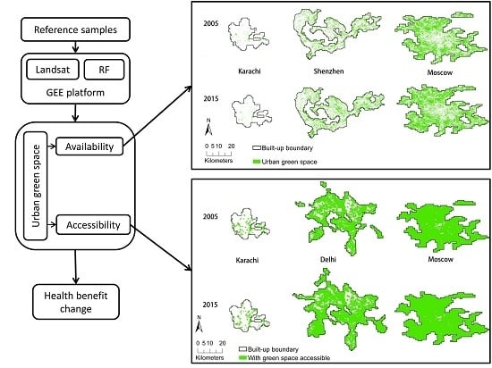
:Urban green spaces can yield considerable health benefits to urban residents. Assessing these health benefits is a key step for managing urban green spaces for human health and wellbeing in cities. In this study, we assessed the change of health benefits generated by urban green spaces in 28 megacities worldwide between 2005 and 2015 by using availability and accessibility as proxy indicators. We first mapped land covers of 28 megacities using 10,823 scenes of Landsat images and a random forest classifier running on Google Earth Engine. We then calculated the availability and accessibility of urban green spaces using the land cover maps and gridded population data. The results showed that the mean availability of urban green spaces in these megacities increased from 27.63% in 2005 to 31.74% in 2015. The mean accessibility of urban green spaces increased from 65.76% in 2005 to 72.86% in 2015. The increased availability and accessibility of urban green spaces in megacities have brought more health benefits to their residents.
1. Introduction
Urban green spaces are important for urban residents’ health [1,2]. Extensive studies have demonstrated that viewing or visiting green spaces can yield positive health effects [1,2,3], such as accelerating recovery from surgery [4], improving cardiovascular health [5], mental health [6], and self-reported general health [7], and lowering all-cause mortality [8]. The mechanism underlying the health benefits of urban green spaces is complex [1] but can largely be attributed to various ecological and social functions of green spaces. Green spaces can contribute to public health through improving air quality, alleviating the urban heat island effect, lowering the level of noise [1,9]. They can also enhance physical activity [10], reduce stress, improve social cohesion [11], and enhance functioning of immune systems [12]. Therefore, maintaining urban green spaces and enhancing their health benefits is an important component of urban health management.
Compositional and structural attributes of urban green spaces are associated with health benefits that urban green spaces can generate, such as availability, accessibility, configuration, and vegetation composition [1,3,13]. Availability measures the quantity of urban green spaces in a city, i.e., the acreage or percentage of urban green spaces [1]. Studies have linked the increased availability of urban green spaces to lowered mortality for residents 35 years old and over in Ontario, Canada [14]. Increased availability was also linked to increased walking for residents in London, UK [15] and physical activity for preschoolers in central Illinois, USA [16] and people in England [17]. Availability also contributed to better mental health of adults in Wisconsin, USA; Adelaide, Australia; and England [18,19,20]. It was found in South Africa that higher availability of urban green spaces was associated with lower incidence of depression for middle-income participants [21,22]. Furthermore, availability of urban green spaces was associated with the general self-reported health outcomes among all age groups in England [23]. Availability of urban green spaces was also inversely associated with coronary heart disease or stroke for adults in Perth, Australia [24].
Accessibility, often measured as the proximity (linear distance or walking distance) of urban green spaces to communities, is also associated with various health benefits such as improved mental health for women in Sweden [25], reduced risk of non-fatal cardiovascular diseases for older adults (aged 45–72 years) in Kaunas, Lithuania [26], and reduced risk of stroke mortality in northwest Florida, USA [27]. Because of the importance of accessibility of urban green spaces, the World Health Organization (WHO) has developed an accessibility indicator for public health [1,3]. The WHO suggests that green spaces with a minimum size of one ha and a maximum distance of 300 m to people’s residence should be used as threshold values for accessibility [1,3]. This indicator provides a reference standard for constructing green spaces for health benefits. Other attributes of urban green spaces, such as vegetation composition (e.g., species richness or biodiversity), have also been associated with human health, mainly mental health [13,28,29]. Studies have shown that high level of species richness or biodiversity in Sheffield [13] and Berlin [29] was related to increased psychological benefits.
Remote sensing has provided a convenient way to monitor the statuses and changes of attributes of urban green spaces. Acreages or percentages of urban green space in cities have been derived from remote sensing data commonly. For example, based on classified Landsat data between 1990 and 2010, the rising trend of urban green coverage in 30 major Chinese cities has been identified [30]. In 111 Southeast Asian cities, it was found that richer cities had more green spaces while cities with higher population densities had less green spaces through classifying Landsat images of these cities [31]. Land cover maps derived using remote sensing data have been used to calculate the accessibility indicator. Liu et al. [32] used SPOT images to assess the change of accessibility of urban green spaces in Beijing and found that accessibility of urban green spaces in Beijing improved notably between 1986 and 2004. Greenness was derived from NDVI and were linked to health outcomes in Ontario, Canada; central Illinois and Wisconsin, USA; and Perth, Australia [14,16,19,24]. Other attributes of urban green spaces that have been retrieved from remotely sensed data include 3D landscape pattern [33,34], urban green volume [35], and tree species composition [36]. Factors such as climatic and socio-economic variables can affect the abundance and dynamic of urban green spaces [30]. For examples, studies have shown that cities with higher population density tended to have less urban green spaces [31,37]. Wealthier (higher per capital GDP) cities tended to have more green spaces [31]. Therefore, to better understand the changes of availability and accessibility of urban green spaces, it is helpful to study the relationships between these driving forces and the detected changes.
Despite the extensive studies on the attributes of urban green spaces, they are rarely studied from the point of view of health. As shown in our early discussion, the attributes of urban green spaces are associated with various health benefits. Therefore, they can be used as coarse proxy indicators for assessing health benefits generated by urban green spaces. The WHO’s suggestion [1,3] on accessibility of urban green spaces reflects this potential well. Due to the wide spatiotemporal coverage and data availability, remote sensing can play an important role in assessing the statuses and dynamics of attributes of urban green spaces, which in turn provides an indirect measure of the change of their health benefits. Nevertheless, thus far, very few studies have addressed this potential. In this study, we used availability and accessibility—two proxy indicators of health benefits generated by urban green spaces—to analyze the change of health benefits provided by urban green spaces in megacities (cities with populations greater than 10 million) worldwide between 2005 and 2015. Specifically, we have the following objectives: (1) to quantify availability of urban green spaces in these cities in 2005 and 2015 with Landsat images and Google Earth Engine (GEE); (2) to calculate accessibility of urban green spaces in these cities in 2005 and 2015 with extracted urban green spaces and population grid data; and (3) to assess changes of availability and accessibility of urban green spaces in these cities between 2005 and 2015 and discuss the influencing factors and possible health implications.
2. Materials and Methods
2.1. Study Area
By 2014, there were 28 megacities according to the United Nation Population Division [38]. We selected all of them as our study area. These megacities are distributed in 18 countries (Figure 1). Their socio-economic and climate conditions are varied (detailed information in Table S1). It is estimated that around one in eight of the world’s urban inhabitants live in these megacities.
2.2. Reference Samples Collection
Reference samples of six types of land covers, including impervious surface, tree/shrub, grass, crop, water, and bare soil, were collected from Landsat images by using high-resolution images on Google Earth as references. We collected 30 to 100 polygons for each class in each megacity for year 2005 and 2015, respectively. In total, 156,478 pixels were collected for 2005 and 205,609 pixels were collected for 2015 as training samples (Table 1). We then uploaded the reference samples to GEE, which is a planetary-scale platform for earth science data and analysis [39]. The samples were used as training samples for land cover classification.
2.3. Landsat Imagery and Feature Extraction on GEE
We used all available standard terrain corrected (L1T) Landsat 5 TM, 7 ETM+ and 8 OLI/TIRS imagery of 2004–2006 (circa 2005), 2014–2016 (circa 2015) with cloud cover <70%. The data format is the pre-processed top of atmosphere (TOA) reflectance Landsat data [39]. We did not use the atmospherically corrected Landsat images in this study because when we performed this study the atmospherically corrected Landsat images had not yet been ingested into GEE platform completely. Winter images were excluded as we mainly focused on the growing seasons. In total, 4452 scenes for 2004–2006 and 6371 scenes for 2014–2016 that covering the study area were used for compositing images and land cover classification.
We used a simple cloud score algorithm available in GEE (https://developers.google.com/earth-engine/landsat) to mask pixels that had high potential of clouds. This algorithm scores Landsat pixels by their relative cloudiness with a value ranging from 0 to 100 [40]. A threshold value of 20 was used to mask the cloudy pixels. We calculated the Normalized difference vegetation index (NDVI) [41], modified normalized difference water index (MNDWI) [42], and Normalized difference built-up index (NDBI) [43] to enhance the information on vegetation, water, and impervious surface. They were used together with the blue, green, red, near infrared, and two shortwave infrared bands of the Landsat image for further processing.
To deal with the inconsistent coverage of clouds, we used percentile-based image compositing method [44,45] to extract selected percentile value of each pixel for each of the nine bands (i.e., blue, green, red, near infrared, shortwave infrared band1-2, NDVI, MNDWI, and NDBI). The percentile-based image compositing method is a pixel-based compositing method, so it is different from the traditional scene-based mosaicking. In this method, all available image values of a specific pixel location for each band were ranked from minimum to maximum. Then values for specific percentiles were selected. For example, the 0 percentile value refers to the minimum value of the pixel for a specific band. This percentile-based compositing method can capture phenology information without any explicit assumption and prior knowledge of the timing of phenology [46]. Land cover classification with good accuracy has been achieved using the percentile based composite method [45,46,47]. In this study, we included percentile values at 0%, 10%, 25%, 50%, 75%, 90% and 100% by following Hansen’s method [45]. In total, 63 features (nine bands multiplied by seven percentile values) were extracted and used for land cover classification.
2.4. Land Cover Classification and Accuracy Assessment
Land cover classification was performed on the GEE platform using random forest (RF) classifier. RF is an ensemble classifier consists of many tree-structured classifiers [48]. RF can handle many training data and variables and keep accuracy when a proportion of data is missing [49,50,51]. In this study, the number of trees was set to 100, and the number of variables per split was set to the square root of the number of variables.
After classification, we extracted 300 pixels from each classified image using a proportional stratified random sampling method. The proportion of pixels sampled in stratum (i.e., a land cover class) was in accordance to the percentage of the land cover class in all land cover types. We also set a minimum sample size of 20 pixels for each class. We then interpreted these validation samples visually on the composited Landsat images and Google Earth high-resolution images. Based on the interpretation result, we estimated the accuracy of classification results.
2.5. Urban Green Space Extraction
We created the border of urban built-up areas for each city from the land cover map. First, we generated single class intensity maps for impervious surface, water bodies, crop, and bare soil. The intensity maps were created using a 1 km by 1 km moving window [52,53] in ArcMap 10.1 (Esri Inc., Redlands, CA, USA). The intensity map was a ratio (0–1) map of a specific type of land cover. Then we used a multiple-criteria approach to determine whether a pixel (1 km resolution) belonged to the urban built-up area. Urban built-up areas usually have a relatively high proportion of impervious surfaces and low proportions of agricultural lands, water, and barren lands. The criteria were: (1) the impervious surface intensity of a pixel was greater than 0.2 [54]; and (2) the sum of water, crop and bare soil of a pixel was less than 0.5. The result was a built-up/non built-up map at 1-km resolution. We then converted the built-up/non built-up map to polygons and excluded small (less than 5 km2) and dispersed polygons. These are mainly dispersed rural settlements. The boundary of built-up areas for each megacity was then generated by choosing the largest built-up polygon and keeping polygons in 2 km from the largest built-up polygon [52,53]. The boundaries were manually modified by referencing to the high-resolution image on Google Earth if necessary. The generated boundaries files were available as supplementary files.
Finally, we extracted out tree/shrub and grass cover within the border of built-up area from the land cover map and merged them as urban green spaces.
2.6. Calculating Availability and Accessibility of Urban Green Spaces
Here, we chose the percentage of urban green spaces to indicate availability of urban green space in each megacity. The percentage of urban green space was calculated as follows:
where PUGS is percentage of urban green space, UGS is area of urban green space, and BUA is area of built-up area.
In this study, we used an accessibility indicator of urban green space proposed by the WHO [1,3]. This indicator is relevant to public health, and is suitable for inter-city comparison. It was calculated as follows [3]:
where AI is accessibility indicator, which measure the proportion of urban population that lives within an accessible distance to urban green spaces. NACC is the number of urban inhabitants who live nearby (in 300 m linear distance) to an urban green space with a size of one ha and over. NTOTAL is the total number of urban inhabitants within the city.
We extracted all patches of urban green spaces that have a size of one ha and over for each megacity. Then, these patches were buffered for 300 m. NACC was calculated by counting the number of population within the boundary of the buffered areas. NTOTAL was calculated by counting the total number of population within the boundary of built-up areas. We obtained the distribution of population in studied cities in 2000 and 2015 from the Global Human Settlement project website (http://ghslsys.jrc.ec.europa.eu/ghs_pop.php) [55]. The data format is 250-m grid data, which are produced by combining the population census data with the built-up grid data of the Global Human Settlement project [55]. We derived the distribution of population in 2005 by using the mean growth rate of population between 2000 and 2015 to extrapolate the population of 2000 to 2005.
2.7. Statistical Analysis
We used the paired t-test to examine whether changes of availability and accessibility indicators of urban green spaces between 2005 and 2015 were significant. We first performed correlation analysis (Supplementary Materials Figure S8) to explore the correlation between explanatory factors (i.e., climatic and socio-economic factors) and availability and accessibility of urban green spaces. Then we performed the multiple general linear model regression analysis to examine the influence of climatic and socio-economic factors on availability and accessibility of urban green spaces. The correlation analysis and general linear regression analysis were performed using package cor.test and lm with R (version 3.3.1; R Development Core Team, Vienna, Austria), respectively. Annual precipitation (AP), annual mean temperature (AMT), population density (PD), and per capita GDP (PCGDP) were included in this study. We chose these climatic and socio-economic variables because they were widely used in studies [30,31] and the data needed for analysis are available. Values of climatic variables were collected from WorldClim [56] and values of socio-economic variables were obtained from Dobbs et al. [57]. Values of these variables for each city can be found in the Supplementary Materials (Table S1). The explanatory variables (AP, AMT, PD and PCGDP) were normalized to avoid differences in the magnitude of these variables before running the multivariate regression analysis. All data analyses were performed using R.
3. Results
3.1. Accuracy Assessment Result
The mean overall accuracy of classification was 90.92 ± 3.26% in 2005 and 88.13 ± 2.78% in 2015. The mean kappa coefficient was 0.87 ± 0.06 and 0.83 ± 0.03 for 2005 and 2015, respectively. The mean overall accuracy of classification met the suggested accuracy for land cover analysis, i.e., 85% [58]. The classified land cover maps and the confusion matrix of classification for each megacity can be found in the Supplementary Materials (Figures S1–S7, and Tables S2–S57).
3.2. Availability of Urban Green Space
Availability of urban green space varied a lot among these megacities (Table 2, Figure 2). One megacity (Moscow) in 2005 and three megacities (London, Paris, and Moscow) in 2015 had more than 50% of urban green space coverage. However, the percentage of urban green spaces in Karachi was less than 5% in both years (3.24% in 2005, 2.73% in 2015).
Overall, the percentage of urban green spaces increased significantly (Difference = 4.11%, p < 0.0001) between 2005 and 2015. However, five megacities, including Los Angeles-Long Beach-Santa Ana, Cairo, Lagos, Karachi, and Osaka, had a slight decrease of the percentage of urban green space.
The results of the multiple general linear model regression showed that availability of urban green spaces in these megacities were highly correlated with the climate factors. Socio-economic factors did not have a significant correlation with availability of green spaces. Megacities with lower AMT and higher AP had significant higher availability of urban green spaces than others (Table 3).
3.3. Accessibility of Urban Green Space
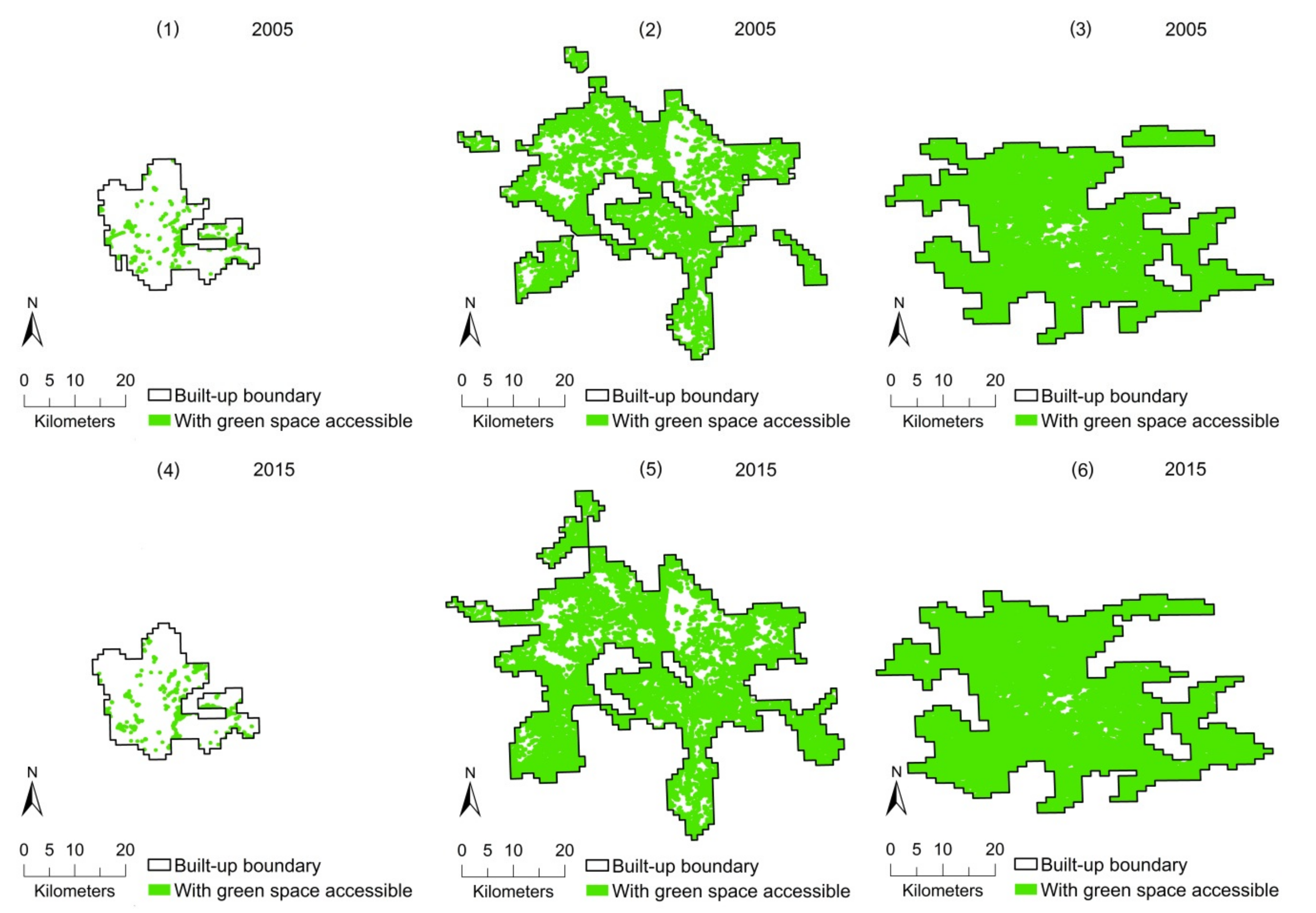
Accessibility of urban green space also varied greatly among these megacities (Table 2 and Figure 3). According to the AI value, less than 12% of the urban populations in Karachi lived within 300 m distance to an urban green space larger than 1 ha in both years. However, in Moscow, nearly all of the urban population met the WHO standard in both years. Totally, there were two megacities in 2005 and five megacities in 2015 where more than 90% of urban inhabitants lived in the 300-m radius of urban green spaces with sizes ≥ 1 ha.
Overall, accessibility of urban green spaces in the megacities increased between 2005 and 2015. Values of AI increased significantly (Difference = 7.10%, p < 0.001) from 65.76% in 2005 to 72.86% in 2015. Values of AI for four cities, Cairo, Lagos, Karachi, and Los Angeles–Long Beach–Santa Ana, decreased between 2005 and 2015.
Similar to availability, accessibility of the 28 cities were significantly affected by climate factors but not socio-economic factors. Megacities with lower AMT and higher AP had significantly higher accessibility of urban green spaces than others (Table 4).
4. Discussion
4.1. Availability of Urban Green Spaces and Changes of Health Benefit
Availability of urban green spaces varied among megacities with different natural and socioeconomic conditions. According to the results of multiple regression analysis, megacities with higher AMT had significantly lower availability of urban green spaces than others (Table 3, Figure S8a). Conversely, megacities with higher AP had significantly higher availability of urban green spaces (Table 3, Figure S8b). Dobbs et al. [59] also found that cities with higher rainfall and lower AMT had higher percentages of green cover for 100 cities worldwide, but the relationship was not significant. Wealthier megacities such as New York–Newark, London, and Moscow tend to have higher availability of urban green spaces (Table 2 and Table S1), but the influence of wealth (per capita GDP) on availability of urban green spaces is not significant. This was partly in agreement with observations by Richards et al. [31], who found that richer cities had more urban green spaces. Availability of urban green spaces in Karachi was the lowest because of its warm and dry climate and relatively low level of economic performance (Table S1). For megacities with the same level of economic performance, climate conditions can significantly influence the availability of urban green spaces. For example, the availability of urban green spaces in New York–Newark was higher than Los Angeles–Long Beach–Santa Ana because the latter had a drier climate (Table 2 and Table S1).
Between 2005 and 2015, the availability of urban green spaces increased by 4.11%. Similar trends are also found in other studies. For 202 European cities, Kabisch and Haase [60] identified an overall increase of 0.54% of urban green spaces annually between 2000 and 2006. Yang et al. [30] found an increase of urban green coverage by a mean annual rate of 1.51% between 1990 and 2010 for 30 major Chinese cities. This pattern may reflect the fact that cities worldwide are increasingly paying attention to create and preserve urban green spaces during development. However, despite the overall increasing trend, there are exceptions. For example, in Los Angeles-Long Beach-Santa Ana, the percentage of urban green spaces decreased from 20.29% in 2005 to 18.20% in 2015. This was in agreement with the analysis of Nowak et al. [61], in which they also found that the tree cover in Los Angeles declined because the tree cover was converted to impervious surfaces and grass cover.
Availability of urban green spaces is closely linked to human health benefits. High availability can increase physical activity [15,16] and improve mental health and general self-reported health [18,23]. The overall increasing trend indicates that the contribution of urban green spaces to residents’ wellbeing in megacities is increasing. However, the contribution varied among megacities and there were gaps among cities. For example, compared to other megacities, residents in Karachi might obtain less health benefits from urban green spaces because availability of urban green spaces in Karachi was the lowest among all studied cities. Unfortunately, due to the high population density [62], severe air pollution [63], and the urban heat island problem [64] in Karachi, the health benefits of urban green spaces are needed more than anywhere. The environmental inequality and its potential health consequence has long been a focus of international development [65]. Clearly, urban greening should be included into an integrated package of urban development for these cities.
4.2. Accessibility of Urban Green Spaces and Changes of Health Benefit
Using the accessibility indicator, we found that accessibility of urban green spaces also varied among megacities. With the lowest availability of urban green spaces, Karachi also had the lowest accessibility of urban green spaces. Less than 12% of urban inhabitants in Karachi were within 300 m of an urban green space with a size ≥ 1 ha. In Moscow, nearly all of the urban inhabitants were within the 300-m radius of urban green spaces with sizes ≥ 1 ha. Usually, accessibility of urban green spaces increased with the availability. However, patch size and distribution of urban green spaces can affect the accessibility of urban green spaces [66]. Large amount of small urban green spaces can provide more even accessibility for urban inhabitants [67]. For example, availability of urban green spaces in Shanghai and Buenos Aires was 32.01% and 34.1% in 2015, respectively. However, values of accessibility in Shanghai and Buenos Aires in 2015 were 85.50% and 72.99%, respectively. It is worth noting that small green spaces may provide less extensive opportunities for recreation so contribute less health benefits than large-size green spaces. The health benefits of many small urban green spaces need to be studied further. Similar to availability, accessibility of urban green spaces was also mainly influenced by climate factors according to the multiple regression analysis. Megacities with higher AP and lower AMT had significantly higher accessibility of urban green spaces than others (Table 4 and Figure S8a,b). With a warmer and drier desert climate condition typical for desert zones, Karachi had a very low accessibility of urban green spaces compared with megacities distributed in the deciduous forest zones (e.g., London, Moscow, New York–Newak) (Table 2 and Table S1).
Overall, accessibility of urban green spaces in megacities has been improved between 2005 and 2015. However, despite the improvement, only a few cities could fully meet the WHO’s standard on accessibility. In Karachi city, more than 85% urban inhabitants could not meet the WHO standard in 2015. Rapid urbanization and loss of urban green spaces in Karachi [68] will make this situation even worse. It is therefore important to improve accessibility in cities that have low accessibility and maintain the high accessibility in cities such as Moscow, London and Paris.
Accessibility is also closely related to health benefits of green spaces [1,3,28]. The overall rising trend of accessibility in the global megacities indicated that urban inhabitants could potentially gain more health benefits from urban green spaces. Similar to the pattern revealed by availability, we found that there were megacities that have experienced a decrease in accessibility, despite the overall increasing trend of accessibility. For example, in parallel with the decrease of availability, accessibility indicator value of Los Angeles-Long Beach-Santa Ana decreased from 56.12% to 52.75% between 2005 and 2015.
4.3. Joint Influences of Availability and Accessibility
We found that changes in accessibility of urban green spaces usually occurred in parallel with changes of availability. However, there were also a few exceptions. For example, the availability of urban green spaces in Osaka decreased slightly (−1.13%), but accessibility of urban green spaces in Osaka increased by 2.46%. This might be due to the change of configurations of urban green spaces in Osaka between 2005 and 2015.
Accessibility is a good supplementary indicator to availability because it can reflect the spatial configuration of urban green spaces (i.e., spatial arrangement and structural characteristics of urban green space patches [69]). For example, De Clercq et al. (2007) [70] examined relationships between spatial pattern of recreational forests and these forests’ accessibility. They found that number of forest patches was positively correlated with accessibility, which indicated that if quantity of forest cover was the same, higher patch density can improve the accessibility. Different configurations of the same quantity of urban green spaces might have different health benefits. For example, a study of the cooling service of urban green spaces with different configuration patterns showed that dispersed urban green spaces can lead to higher overall regional cooling than clustered green spaces, although the clustered green spaces can enhance local cooling [71].
To improve the health benefits contributed by urban green spaces, cities can increase the amount of urban green spaces, i.e., their availability. At the same time, accessibility can be improved by allocating small- and medium-size urban green spaces more evenly rather than pouring all resources into building few big and clustered green spaces [66,72].
Providing universal access to urban green spaces is already a target of the sustainable development goals (SDGs) adopted by the international society in 2015: “By 2030, provide universal access to safe, inclusive and accessible, green and public spaces, in particular for women and children, older persons and persons with disabilities” [73]. Due to the symbolic importance of megacities, there is an urgent need to improve both availability and accessibility of urban green spaces to realize this goal, especially for these megacities that are falling behind.
4.4. Limitations of the Current Study
We combined the availability and accessibility indicators to assess the change of health benefits generated by urban green spaces in megacities in the last decade. In this study, we focused on the physical dimension of these two indicators because they can be conveniently derived from remotely sensed data. However, one must realize that these two indicators also contain socioeconomic dimensions. The availability and accessibility indicators used in this study can roughly reflect the use of green spaces by people but cannot quantify the use accurately. For example, increased availability of urban green spaces was commonly associated with increased physical activity. However, how many people actually used the urban green spaces for physical activity were not clear. Urban residents may even not have access to a nearby green space due to social exclusion [65]. For example, some green spaces (e.g., private gardens) were not publicly accessible. Although these green spaces can yield health benefits, the amount of urban inhabitants they served is less than public green spaces. This shows the limitation of using remote sensing to study the health benefits of urban green spaces. Remote sensing can track the spatiotemporal changes of biophysical features of urban green spaces. However, it is difficult to use remote sensing, especially medium-resolution remote sensing data, to track human activities occurring in urban green spaces and associated health benefits. It is also difficult to quantify the quality of urban green space using remote sensing data [23], which might influence health benefits, especially the benefit to mental health [28]. Furthermore, urban green space maps derived from medium or coarse resolution remote sensing data cannot capture small patches of urban green spaces [74], which have important health benefits too. Therefore, as we discussed in the introduction, availability and accessibility of urban green spaces derived using a remote sensing approach can only be viewed as coarse proxy indicators of health benefits from urban green spaces. Despite these limitations, remote sensing data can play an important role in assessing statuses and changes of attributes of urban green spaces that have proved links with human health. This is especially useful for conducting large-scale inter-city comparisons. Except for adopting finer remotely sensed data and population data, a better understanding of health benefits from urban green spaces can be obtained by combining remotely sensed data with social sensing data such as point of interest data and with health monitoring data provided by wearable sensors.
5. Conclusions
Urban green spaces can bring considerable health benefits to urban inhabitants. Due to the large population of megacities, the health benefits generated from urban green spaces are especially valuable. Assessing the magnitude and spatial distribution of these benefits is therefore important for planning and designing urban green spaces to generate more health benefits. In this study, we developed a method based on remote sensing data to conduct a quick assessment of the potential supply of health benefits by urban green spaces in 28 megacities. We used two indicators to quantify availability and accessibility of urban green spaces in these cities. Our analysis utilized a large amount of Landsat images and the RF classifier provided by the GEE platform, which allowed us to obtain accurate estimate of statuses and dynamics of attributes of urban green spaces in these cities. Our results showed that overall both availability and accessibility of urban green spaces in these cities increased between 2005 and 2015. We thus inferred that more residents in these cities enjoyed the health benefits generated by urban green spaces in this period. At the same time, we noted that there were a few megacities (e.g., Karachi) that showed declining trends of availability and accessibility. In the future, to build more green spaces and preserve existing ones should be a priority in these cities. The action can be included into an integrative urban health management package. The information produced by this study can help these megacities to adjust their management of urban green spaces to achieve the target included in SDGs.
Supplementary Materials
The following are available online at www.mdpi.com/2072-4292/9/12/1266/s1, Table S1: Values of climatic variables and socioeconomic variables of the 28 megacities, Tables S2–S57: Confusion matrix of classification, Figures S1–S7: Classification maps of megacities, Figure S8: Correlations between: availability (a–d); and accessibility (e–h) of urban green spaces and climatic and socio-economic variables, and built-up boundary files.
Acknowledgments
We want to thank Nicholas Clinton from Google for providing us free access to Google Earth Engine and for helping us with technical issues. This study was supported by National Natural Science Foundation of China (Grant number 31570458, 2016) and National High Technology Research and Development Program (Grant number 2013AA122804, 2013–2016).
Author Contributions
Jun Yang designed the study and contributed to writing. Conghong Huang conducted data analysis and wrote the paper. Hui Lu contributed to writing. Huabing Huang contributed to writing. Le Yu contributed to writing.
Conflicts of Interest
The authors declare no conflict of interest.
References
- World Health Organization (WHO). Urban Green Spaces and Health: A Review of Evidence; World Health Organization: Geneva, Switzerland, 2016. [Google Scholar]
- Hartig, T.; Mitchell, R.; De Vries, S.; Frumkin, H. Nature and health. Annu. Rev. Public Health 2014, 35, 207–228. [Google Scholar] [CrossRef] [PubMed]
- Annerstedt van den Bosch, M.; Mudu, P.; Uscila, V.; Barrdahl, M.; Kulinkina, A.; Staatsen, B.; Swart, W.; Kruize, H.; Zurlyte, I.; Egorov, A.I. Development of an urban green space indicator and the public health rationale. Scand. J. Soc. Med. 2016, 44, 159–167. [Google Scholar] [CrossRef] [PubMed]
- Ulrich, R. View through a window may influence recovery. Science 1984, 224, 224–225. [Google Scholar] [CrossRef]
- Paquet, C.; Orschulok, T.P.; Coffee, N.T.; Howard, N.J.; Hugo, G.; Taylor, A.W.; Adams, R.J.; Daniel, M. Are accessibility and characteristics of public open spaces associated with a better cardiometabolic health? Landsc. Urban Plan. 2013, 118, 70–78. [Google Scholar] [CrossRef]
- Sturm, R.; Cohen, D. Proximity to urban parks and mental health. J. Ment. Health Policy Econ. 2014, 17, 19–24. [Google Scholar] [PubMed]
- Maas, J.; Verheij, R.A.; Groenewegen, P.P.; De Vries, S.; Spreeuwenberg, P. Green space, urbanity, and health: How strong is the relation? J. Epidemiol. Community Health 2006, 60, 587–592. [Google Scholar] [CrossRef] [PubMed]
- Mitchell, R.; Popham, F. Effect of exposure to natural environment on health inequalities: An observational population study. Lancet 2008, 372, 1655–1660. [Google Scholar] [CrossRef]
- Gidlöf-Gunnarsson, A.; Öhrström, E. Noise and well-being in urban residential environments: The potential role of perceived availability to nearby green areas. Landsc. Urban Plan. 2007, 83, 115–126. [Google Scholar] [CrossRef]
- Zhang, W.; Yang, J.; Ma, L.; Huang, C. Factors affecting the use of urban green spaces for physical activities: Views of young urban residents in beijing. Urban For. Urban Green. 2015, 14, 851–857. [Google Scholar] [CrossRef]
- De Vries, S.; van Dillen, S.M.; Groenewegen, P.P.; Spreeuwenberg, P. Streetscape greenery and health: Stress, social cohesion and physical activity as mediators. Soc. Sci. Med. 2013, 94, 26–33. [Google Scholar] [CrossRef] [PubMed]
- Kuo, M. How might contact with nature promote human health? Promising mechanisms and a possible central pathway. Front. Psychol. 2015, 6, 1093. [Google Scholar] [CrossRef] [PubMed]
- Fuller, R.A.; Irvine, K.N.; Devine-Wright, P.; Warren, P.H.; Gaston, K.J. Psychological benefits of greenspace increase with biodiversity. Biol. Lett. 2007, 3, 390–394. [Google Scholar] [CrossRef] [PubMed]
- Villeneuve, P.J.; Jerrett, M.; Su, J.G.; Burnett, R.T.; Chen, H.; Wheeler, A.J.; Goldberg, M.S. A cohort study relating urban green space with mortality in ontario, canada. Environ. Res. 2012, 115, 51–58. [Google Scholar] [CrossRef] [PubMed]
- Sarkar, C.; Webster, C.; Pryor, M.; Tang, D.; Melbourne, S.; Zhang, X.; Jianzheng, L. Exploring associations between urban green, street design and walking: Results from the greater london boroughs. Landsc. Urban Plan. 2015, 143, 112–125. [Google Scholar] [CrossRef]
- Grigsby-Toussaint, D.S.; Chi, S.-H.; Fiese, B.H. Where they live, how they play: Neighborhood greenness and outdoor physical activity among preschoolers. Int. J. Health Geogr. 2011, 10, 66. [Google Scholar] [CrossRef] [PubMed]
- Mytton, O.T.; Townsend, N.; Rutter, H.; Foster, C. Green space and physical activity: An observational study using health survey for england data. Health Place 2012, 18, 1034–1041. [Google Scholar] [CrossRef] [PubMed]
- Alcock, I.; White, M.P.; Wheeler, B.W.; Fleming, L.E.; Depledge, M.H. Longitudinal effects on mental health of moving to greener and less green urban areas. Environ. Sci. Technol. 2014, 48, 1247–1255. [Google Scholar] [CrossRef] [PubMed] [Green Version]
- Beyer, K.M.; Kaltenbach, A.; Szabo, A.; Bogar, S.; Nieto, F.J.; Malecki, K.M. Exposure to neighborhood green space and mental health: Evidence from the survey of the health of wisconsin. Int. J. Environ. Res. Public Health 2014, 11, 3453–3472. [Google Scholar] [CrossRef] [PubMed]
- Sugiyama, T.; Leslie, E.; Giles-Corti, B.; Owen, N. Associations of neighbourhood greenness with physical and mental health: Do walking, social coherence and local social interaction explain the relationships? J. Epidemiol. Community Health 2008, 62. [Google Scholar] [CrossRef]
- Craig, J.M.; Prescott, S.L. Planning ahead: The mental health value of natural environments. Lancet Planet. Health 2017, 1, e128–e129. [Google Scholar] [CrossRef]
- Tomita, A.; Vandormael, A.M.; Cuadros, D.; Di Minin, E.; Heikinheimo, V.; Tanser, F.; Slotow, R.; Burns, J.K. Green environment and incident depression in south africa: A geospatial analysis and mental health implications in a resource-limited setting. Lancet Planet. Health 2017, 1, e152–e162. [Google Scholar] [CrossRef]
- Mitchell, R.; Popham, F. Greenspace, urbanity and health: Relationships in england. J. Epidemiol. Community Health 2007, 61, 681–683. [Google Scholar] [CrossRef] [PubMed]
- Pereira, G.; Foster, S.; Martin, K.; Christian, H.; Boruff, B.J.; Knuiman, M.; Giles-Corti, B. The association between neighborhood greenness and cardiovascular disease: An observational study. BMC Public Health 2012, 12, 466. [Google Scholar] [CrossRef] [PubMed]
- Van den Bosch, M.A.; Östergren, P.-O.; Grahn, P.; Skärbäck, E.; Währborg, P. Moving to serene nature may prevent poor mental health—Results from a swedish longitudinal cohort study. Int. J. Environ. Res. Public Health 2015, 12, 7974–7989. [Google Scholar] [CrossRef] [PubMed]
- Tamosiunas, A.; Grazuleviciene, R.; Luksiene, D.; Dedele, A.; Reklaitiene, R.; Baceviciene, M.; Vencloviene, J.; Bernotiene, G.; Radisauskas, R.; Malinauskiene, V. Accessibility and use of urban green spaces, and cardiovascular health: Findings from a kaunas cohort study. Environ. Health 2014, 13, 20. [Google Scholar] [CrossRef] [PubMed]
- Hu, Z.; Liebens, J.; Rao, K.R. Linking stroke mortality with air pollution, income, and greenness in northwest florida: An ecological geographical study. Int. J. Health Geogr. 2008, 7, 20. [Google Scholar] [CrossRef] [PubMed]
- Ekkel, E.D.; de Vries, S. Nearby green space and human health: Evaluating accessibility metrics. Landsc. Urban Plan. 2017, 157, 214–220. [Google Scholar] [CrossRef]
- Honold, J.; Lakes, T.; Beyer, R.; van der Meer, E. Restoration in urban spaces: Nature views from home, greenways, and public parks. Environ. Behav. 2016, 48, 796–825. [Google Scholar] [CrossRef]
- Yang, J.; Huang, C.; Zhang, Z.; Wang, L. The temporal trend of urban green coverage in major chinese cities between 1990 and 2010. Urban For. Urban Green. 2014, 13, 19–27. [Google Scholar] [CrossRef]
- Richards, D.R.; Passy, P.; Oh, R.R. Impacts of population density and wealth on the quantity and structure of urban green space in tropical southeast asia. Landsc. Urban Plan. 2017, 157, 553–560. [Google Scholar] [CrossRef]
- Liu, Z.; Mao, F.; Zhou, W.; Li, Q.; Huang, J.; Zhu, X. Accessibility assessment of urban green space: A quantitative perspective. In Proceedings of the IEEE International Geoscience and Remote Sensing Symposium (IGARSS 2008), Boston, MA, USA, 6–11 July 2008; pp. 1314–1317. [Google Scholar]
- Chen, Z.; Xu, B.; Devereux, B. Urban landscape pattern analysis based on 3d landscape models. Appl. Geogr. 2014, 55, 82–91. [Google Scholar] [CrossRef]
- Chen, Z.; Xu, B. Enhancing urban landscape configurations by integrating 3d landscape pattern analysis with people’s landscape preferences. Environ. Earth Sci. 2016, 75, 1018. [Google Scholar] [CrossRef]
- Casalegno, S.; Anderson, K.; Cox, D.T.; Hancock, S.; Gaston, K.J. Ecological connectivity in the three-dimensional urban green volume using waveform airborne lidar. Sci. Rep. 2017, 7, 45571. [Google Scholar] [CrossRef] [PubMed]
- Pu, R.; Landry, S. A comparative analysis of high spatial resolution ikonos and worldview-2 imagery for mapping urban tree species. Remote Sens. Environ. 2012, 124, 516–533. [Google Scholar] [CrossRef]
- Fuller, R.A.; Gaston, K.J. The scaling of green space coverage in european cities. Biol. Lett. 2009, 5, 352–355. [Google Scholar] [CrossRef] [PubMed]
- United Nations. World Urbanization Prospects: The 2014 Revision; Department of Economic and Social Affairs, Population Division, United Nations: New York, NY, USA, 2014. [Google Scholar]
- Gorelick, N.; Hancher, M.; Dixon, M.; Ilyushchenko, S.; Thau, D.; Moore, R. Google earth engine: Planetary-scale geospatial analysis for everyone. Remote Sens. Environ. 2017. [Google Scholar] [CrossRef]
- Huang, H.; Chen, Y.; Clinton, N.; Wang, J.; Wang, X.; Liu, C.; Gong, P.; Yang, J.; Bai, Y.; Zheng, Y. Mapping major land cover dynamics in beijing using all landsat images in google earth engine. Remote Sens. Environ. 2017. [Google Scholar] [CrossRef]
- Tucker, C.J. Red and photographic infrared linear combinations for monitoring vegetation. Remote Sens. Environ. 1979, 8, 127–150. [Google Scholar] [CrossRef]
- Xu, H. Modification of normalised difference water index (ndwi) to enhance open water features in remotely sensed imagery. Int. J. Remote Sens. 2006, 27, 3025–3033. [Google Scholar] [CrossRef]
- Zha, Y.; Gao, J.; Ni, S. Use of normalized difference built-up index in automatically mapping urban areas from tm imagery. Int. J. Remote Sens. 2003, 24, 583–594. [Google Scholar] [CrossRef]
- Hansen, M.C.; Potapov, P.V.; Moore, R.; Hancher, M.; Turubanova, S.; Tyukavina, A.; Thau, D.; Stehman, S.; Goetz, S.; Loveland, T. High-resolution global maps of 21st-century forest cover change. Science 2013, 342, 850–853. [Google Scholar] [CrossRef] [PubMed]
- Sharma, R.C.; Tateishi, R.; Hara, K.; Iizuka, K. Production of the japan 30-m land cover map of 2013–2015 using a random forests-based feature optimization approach. Remote Sens. 2016, 8, 429. [Google Scholar] [CrossRef]
- Azzari, G.; Lobell, D. Landsat-based classification in the cloud: An opportunity for a paradigm shift in land cover monitoring. Remote Sens. Environ. 2017. [Google Scholar] [CrossRef]
- Song, X.-P.; Potapov, P.V.; Krylov, A.; King, L.; Di Bella, C.M.; Hudson, A.; Khan, A.; Adusei, B.; Stehman, S.V.; Hansen, M.C. National-scale soybean mapping and area estimation in the united states using medium resolution satellite imagery and field survey. Remote Sens. Environ. 2017, 190, 383–395. [Google Scholar] [CrossRef]
- Breiman, L. Random forests. Mach. Learn. 2001, 45, 5–32. [Google Scholar] [CrossRef]
- Johansen, K.; Phinn, S.; Taylor, M. Mapping woody vegetation clearing in queensland, australia from landsat imagery using the google earth engine. Remote Sens. Appl. Soc. Environ. 2015, 1, 36–49. [Google Scholar] [CrossRef]
- Li, X.; Gong, P.; Liang, L. A 30-year (1984–2013) record of annual urban dynamics of beijing city derived from landsat data. Remote Sens. Environ. 2015, 166, 78–90. [Google Scholar] [CrossRef]
- Wang, J.; Li, C.; Hu, L.; Zhao, Y.; Huang, H.; Gong, P. Seasonal land cover dynamics in beijing derived from landsat 8 data using a spatio-temporal contextual approach. Remote Sens. 2015, 7, 865–881. [Google Scholar] [CrossRef]
- Zhou, D.; Zhao, S.; Liu, S.; Zhang, L.; Zhu, C. Surface urban heat island in china’s 32 major cities: Spatial patterns and drivers. Remote Sens. Environ. 2014, 152, 51–61. [Google Scholar] [CrossRef]
- Zhou, D.; Zhao, S.; Zhang, L.; Liu, S. Remotely sensed assessment of urbanization effects on vegetation phenology in china’s 32 major cities. Remote Sens. Environ. 2016, 176, 272–281. [Google Scholar] [CrossRef]
- Zhou, Y.; Smith, S.J.; Zhao, K.; Imhoff, M.; Thomson, A.; Bond-Lamberty, B.; Asrar, G.R.; Zhang, X.; He, C.; Elvidge, C.D. A global map of urban extent from nightlights. Environ. Res. Lett. 2015, 10. [Google Scholar] [CrossRef]
- European Commission, Joint Research Centre (JRC); Columbia University, Center for International Earth Science Information Network. GHS Population Grid, Derived from GPW4, Multitemporal (1975, 1990, 2000, 2015). Available online: http://data.Europa.Eu/89h/jrc-ghsl-ghs_pop_gpw4_globe_r2015a (accessed on 28 June 2017).
- Hijmans, R.J.; Cameron, S.E.; Parra, J.L.; Jones, P.G.; Jarvis, A. Very high resolution interpolated climate surfaces for global land areas. Int. J. Climatol. 2005, 25, 1965–1978. [Google Scholar] [CrossRef]
- Dobbs, R.; Smit, S.; Remes, J.; Manyika, J.; Roxburgh, C.; Restrepo, A. Urban World: Mapping the Economic Power of Cities; McKinsey Global Institute: Seoul, Korea, 2011. [Google Scholar]
- Thomlinson, J.R.; Bolstad, P.V.; Cohen, W.B. Coordinating methodologies for scaling landcover classifications from site-specific to global: Steps toward validating global map products. Remote Sens. Environ. 1999, 70, 16–28. [Google Scholar] [CrossRef]
- Dobbs, C.; Nitschke, C.; Kendal, D. Assessing the drivers shaping global patterns of urban vegetation landscape structure. Sci. Total Environ. 2017, 592, 171–177. [Google Scholar] [CrossRef] [PubMed]
- Kabisch, N.; Haase, D. Green spaces of european cities revisited for 1990–2006. Landsc. Urban Plan. 2013, 110, 113–122. [Google Scholar] [CrossRef]
- Nowak, D.J.; Greenfield, E.J. Tree and impervious cover change in us cities. Urban For. Urban Green. 2012, 11, 21–30. [Google Scholar] [CrossRef]
- Qureshi, S. The fast growing megacity karachi as a frontier of environmental challenges: Urbanization and contemporary urbanism issues. J. Geogr. Reg. Plan. 2010, 3, 306–321. [Google Scholar]
- Khwaja, H.A.; Fatmi, Z.; Malashock, D.; Aminov, Z.; Kazi, A.; Siddique, A.; Qureshi, J.; Carpenter, D.O. Effect of air pollution on daily morbidity in karachi, pakistan. J. Local Glob. Health Sci. 2013, 3, 1–13. [Google Scholar] [CrossRef]
- Sajjad, S.H.; Blond, N.; Batool, R.; Shirazi, S.A.; Shakrullah, K.; Bhalli, M.N. Study of urban heat island of karachi by using finite volume mesoscale model. J. Basic Appl. Sci. 2015, 11, 101–105. [Google Scholar] [CrossRef]
- Wolch, J.R.; Byrne, J.; Newell, J.P. Urban green space, public health, and environmental justice: The challenge of making cities ‘just green enough’. Landsc. Urban Plan. 2014, 125, 234–244. [Google Scholar] [CrossRef]
- Peschardt, K.K.; Schipperijn, J.; Stigsdotter, U.K. Use of small public urban green spaces (spugs). Urban For. Urban Green. 2012, 11, 235–244. [Google Scholar] [CrossRef]
- Yu, Z.; Wang, Y.; Deng, J.; Shen, Z.; Wang, K.; Zhu, J.; Gan, M. Dynamics of hierarchical urban green space patches and implications for management policy. Sensors 2017, 17, 1304. [Google Scholar] [CrossRef] [PubMed]
- Qureshi, S.; Kazmi, S.J.H.; Breuste, J.H. Ecological disturbances due to high cutback in the green infrastructure of karachi: Analyses of public perception about associated health problems. Urban For. Urban Green. 2010, 9, 187–198. [Google Scholar] [CrossRef]
- Connors, J.P.; Galletti, C.S.; Chow, W.T. Landscape configuration and urban heat island effects: Assessing the relationship between landscape characteristics and land surface temperature in phoenix, arizona. Landsc. Ecol. 2013, 28, 271–283. [Google Scholar] [CrossRef]
- De Clercq, E.M.; De Wulf, R.; Van Herzele, A. Relating spatial pattern of forest cover to accessibility. Landsc. Urban Plan. 2007, 80, 14–22. [Google Scholar] [CrossRef]
- Zhang, Y.; Murray, A.T.; Turner, B. Optimizing green space locations to reduce daytime and nighttime urban heat island effects in phoenix, arizona. Landsc. Urban Plan. 2017, 165, 162–171. [Google Scholar] [CrossRef]
- Haaland, C.; van den Bosch, C.K. Challenges and strategies for urban green-space planning in cities undergoing densification: A review. Urban For. Urban Green. 2015, 14, 760–771. [Google Scholar] [CrossRef]
- United Nations. Sustainable Development Goals. Available online: Http://www.Un.Org/sustainabledevelopment/sustainable-development-goals/ (accessed on 28 June 2017).
- Van den Berg, A.E.; Maas, J.; Verheij, R.A.; Groenewegen, P.P. Green space as a buffer between stressful life events and health. Soc. Sci. Med. 2010, 70, 1203–1210. [Google Scholar] [CrossRef] [PubMed]
Figure 1.
Distribution of the 28 megacities included in this study.
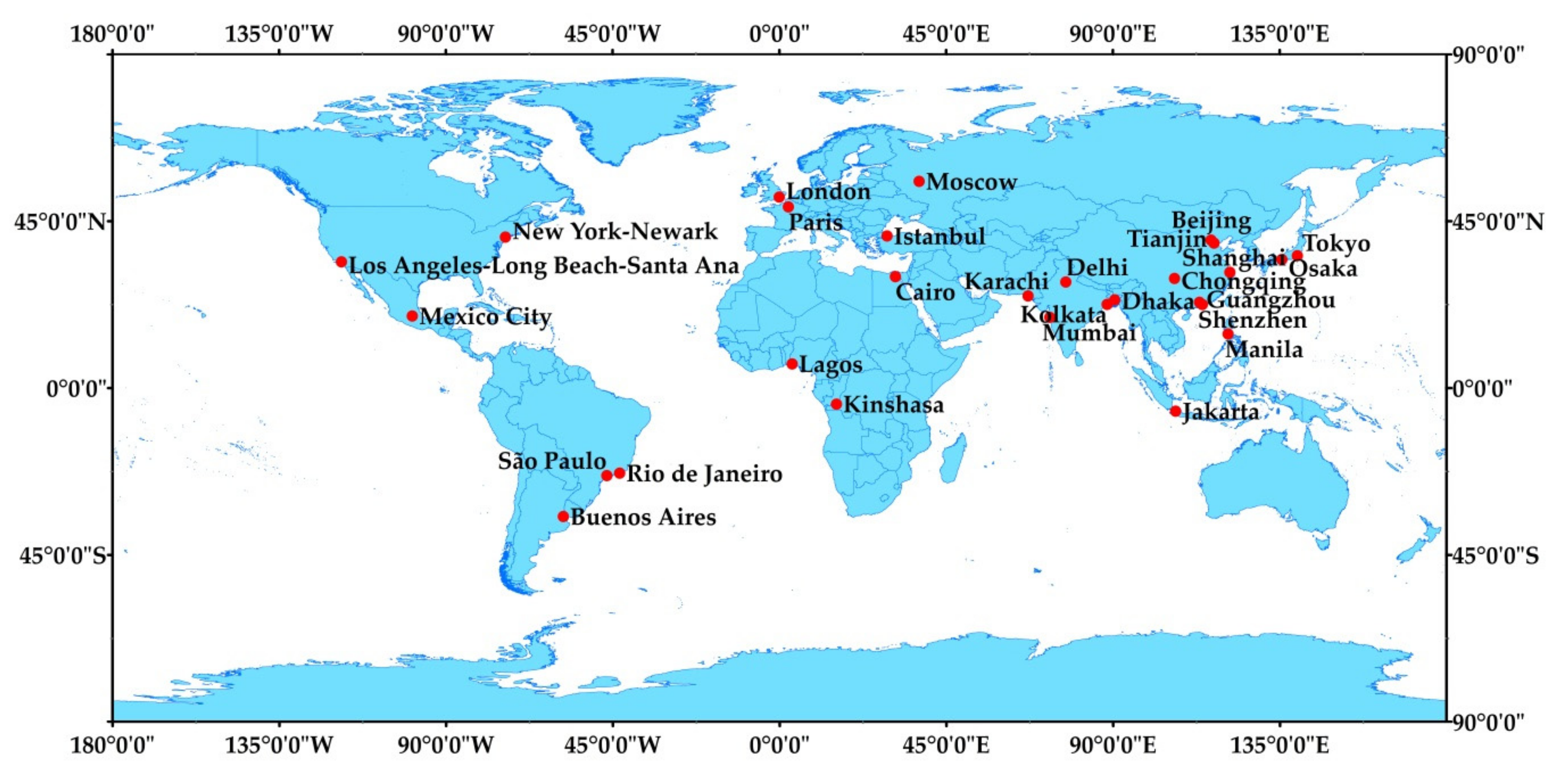
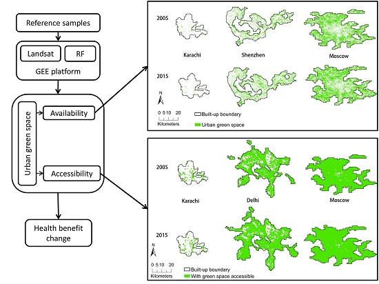
Figure 2.
Distributions of urban green spaces in 2005 and 2015, examples of: the least green (Karachi) (1), median green (Shenzhen) (2), and greenest (Moscow) (3) megacity in 2005; and the least green (Karachi) (4), median green (Shenzhen) (5), and greenest (Moscow) (6) megacity in 2015.
Figure 2.
Distributions of urban green spaces in 2005 and 2015, examples of: the least green (Karachi) (1), median green (Shenzhen) (2), and greenest (Moscow) (3) megacity in 2005; and the least green (Karachi) (4), median green (Shenzhen) (5), and greenest (Moscow) (6) megacity in 2015.
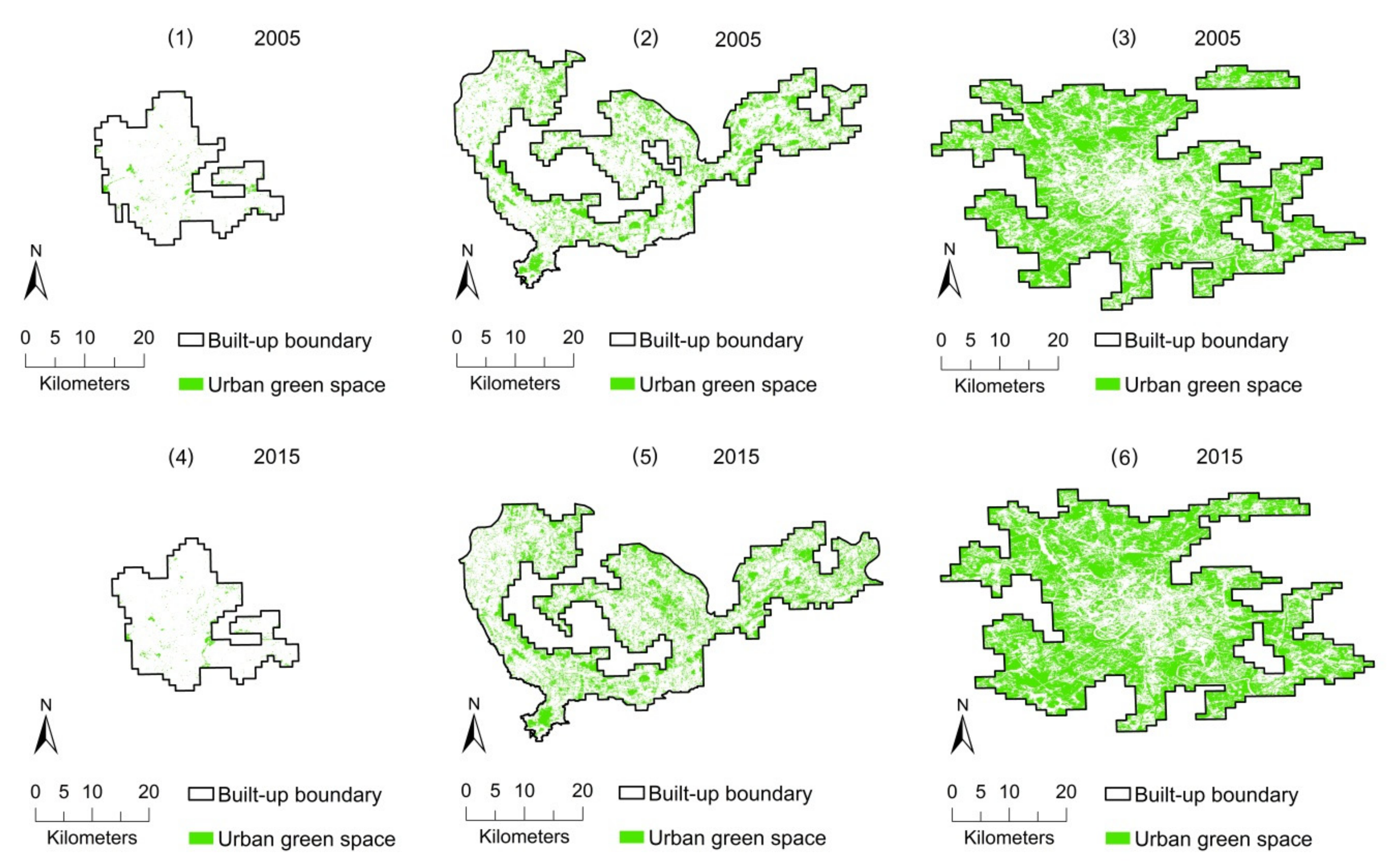
Figure 3.
Distribution of urban green spaces (≥1 ha) and their 300 m buffered areas, examples for megacities of: low (Karachi) (1), median (Delhi) (2), and high (Moscow) (3) values of accessibility indicator in 2005; and low (Karachi) (4), median (Delhi) (5), and high (Moscow) (6) values of accessibility indicator in 2015.

Table 1.
The number of training samples for land cover classification.
| Class Type | 2005 | 2015 | ||
|---|---|---|---|---|
| Number of Polygons or Sites | Number of Pixels | Number of Polygons or Sites | Number of Pixels | |
| Bare soil | 2008 | 9840 | 2616 | 15,643 |
| Crop | 2581 | 9717 | 3364 | 15,408 |
| Grass | 2886 | 14,615 | 3761 | 21,213 |
| Impervious surfaces | 4818 | 72,404 | 6279 | 85,196 |
| Tree/shrub | 4610 | 37,474 | 6007 | 48,482 |
| Water | 2294 | 12,428 | 2990 | 19,667 |
| Sum | 19,197 | 156,478 | 25,018 | 205,609 |
Table 2.
Availability and accessibility of urban green spaces for the 28 megacities in 2005 and 2015.
Table 2.
Availability and accessibility of urban green spaces for the 28 megacities in 2005 and 2015.
| Megacity | PUGS (%) | AI (%) | ||||
|---|---|---|---|---|---|---|
| 2005 | 2015 | Δ05–15 | 2005 | 2015 | Δ05–15 | |
| Los Angeles-Long Beach-Santa Ana | 20.29 | 18.20 | −2.09 | 56.12 | 52.75 | −3.37 |
| Mexico City | 21.70 | 28.00 | 6.30 | 52.21 | 57.81 | 5.60 |
| New York-Newark | 41.72 | 44.56 | 2.84 | 73.36 | 78.34 | 4.98 |
| Rio de Janeiro | 37.86 | 38.43 | 0.57 | 78.59 | 80.08 | 1.48 |
| São Paulo | 27.40 | 30.15 | 2.75 | 67.92 | 71.46 | 3.54 |
| Buenos Aires | 32.99 | 34.10 | 1.11 | 71.83 | 72.99 | 1.16 |
| London | 46.38 | 58.42 | 12.04 | 95.66 | 98.53 | 2.88 |
| Paris | 42.30 | 52.50 | 10.20 | 83.70 | 91.66 | 7.96 |
| Moscow | 52.79 | 56.61 | 3.82 | 98.51 | 99.25 | 0.75 |
| Istanbul | 23.70 | 28.95 | 5.25 | 59.60 | 68.07 | 8.46 |
| Cairo | 12.15 | 11.83 | −0.32 | 32.28 | 27.79 | −4.49 |
| Lagos | 20.17 | 18.55 | −1.62 | 61.54 | 57.76 | −3.78 |
| Kinshasa | 9.32 | 23.53 | 14.21 | 26.78 | 55.60 | 28.82 |
| Karachi | 3.24 | 2.73 | −0.51 | 11.57 | 10.84 | −0.72 |
| Delhi | 26.01 | 32.47 | 6.46 | 69.41 | 75.19 | 5.78 |
| Mumbai | 26.01 | 27.63 | 1.62 | 77.15 | 80.23 | 3.08 |
| Kolkata | 29.34 | 35.21 | 5.87 | 77.78 | 89.06 | 11.28 |
| Dhaka | 17.10 | 20.9 | 3.80 | 62.48 | 68.86 | 6.37 |
| Beijing | 33.88 | 41.82 | 7.94 | 77.91 | 91.97 | 14.06 |
| Tianjin | 21.35 | 23.44 | 2.09 | 60.09 | 74.02 | 13.93 |
| Chongqing | 35.97 | 47.58 | 11.61 | 78.22 | 98.32 | 20.09 |
| Shanghai | 31.11 | 32.01 | 0.90 | 63.19 | 85.50 | 22.30 |
| Guangzhou | 28.70 | 36.08 | 7.38 | 59.11 | 76.42 | 17.31 |
| Shenzhen | 24.74 | 30.05 | 5.31 | 70.44 | 83.93 | 13.50 |
| Manila | 24.69 | 31.82 | 7.13 | 67.40 | 74.84 | 7.44 |
| Jakarta | 34.87 | 36.03 | 1.16 | 85.60 | 86.92 | 1.33 |
| Osaka | 22.50 | 21.37 | −1.13 | 56.67 | 59.14 | 2.46 |
| Tokyo | 25.32 | 25.85 | 0.53 | 66.08 | 72.77 | 6.69 |
| Average | 27.63 | 31.74 | 4.11 | 65.76 | 72.86 | 7.10 |
PUGS: Percentage of urban green space; AI: Accessibility indicator of urban green space.
Table 3.
Results of multiple general linear model regression for availability in 2005 and 2015.
| Factor | 2005 | 2015 | ||||||
|---|---|---|---|---|---|---|---|---|
| Coefficient | SE | t | p | Coefficient | SE | t | p | |
| Intercept | 27.629 | 1.609 | 17.175 | <0.001 | 31.744 | 1.964 | 16.165 | <0.001 |
| Annual mean temperature | −7.164 | 3.017 | −2.374 | 0.026 | −9.715 | 3.683 | −2.638 | 0.015 |
| Annual precipitation | 4.733 | 2.032 | 2.329 | 0.029 | 6.142 | 2.481 | 2.476 | 0.021 |
| Population density | −0.597 | 2.292 | −0.261 | 0.797 | 0.009 | 2.798 | 0.003 | 0.998 |
| Per capita GDP | 1.642 | 2.687 | 0.611 | 0.547 | 0.375 | 3.28 | 0.114 | 0.91 |
SE: Standard error.
Table 4.
Results of multiple general linear model regression for accessibility in 2005 and 2015.
| Factor | 2005 | 2015 | ||||||
|---|---|---|---|---|---|---|---|---|
| Coefficient | SE | t | p | Coefficient | SE | t | p | |
| Intercept | 66.349 | 3.042 | 21.812 | <0.001 | 73.263 | 3.061 | 23.937 | <0.001 |
| Annual mean temperature | −11.998 | 5.705 | −2.103 | 0.047 | −16.215 | 5.74 | −2.825 | 0.01 |
| Annual precipitation | 11.197 | 3.843 | 2.914 | 0.008 | 13.561 | 3.867 | 3.507 | 0.002 |
| Population density | 0.39 | 4.334 | 0.09 | 0.929 | −1.859 | 4.361 | −0.426 | 0.674 |
| Per capita GDP | 1.703 | 5.08 | 0.335 | 0.74 | −3.888 | 5.112 | −0.761 | 0.455 |
SE: Standard error.
© 2017 by the authors. Licensee MDPI, Basel, Switzerland. This article is an open access article distributed under the terms and conditions of the Creative Commons Attribution (CC BY) license (http://creativecommons.org/licenses/by/4.0/).
Share and Cite
MDPI and ACS Style
Huang, C.; Yang, J.; Lu, H.; Huang, H.; Yu, L. Green Spaces as an Indicator of Urban Health: Evaluating Its Changes in 28 Mega-Cities. Remote Sens. 2017, 9, 1266. https://doi.org/10.3390/rs9121266
AMA Style
Huang C, Yang J, Lu H, Huang H, Yu L. Green Spaces as an Indicator of Urban Health: Evaluating Its Changes in 28 Mega-Cities. Remote Sensing. 2017; 9(12):1266. https://doi.org/10.3390/rs9121266
Chicago/Turabian StyleHuang, Conghong, Jun Yang, Hui Lu, Huabing Huang, and Le Yu. 2017. "Green Spaces as an Indicator of Urban Health: Evaluating Its Changes in 28 Mega-Cities" Remote Sensing 9, no. 12: 1266. https://doi.org/10.3390/rs9121266
Note that from the first issue of 2016, this journal uses article numbers instead of page numbers. See further details here.