Improved Atmospheric Modelling of the Oasis-Desert System in Central Asia Using WRF with Actual Satellite Products
by
 , ,
, ,
Miao Zhang
1,2,3,4,5 ,
,
Geping Luo
1,3,*,
Philippe De Maeyer
2,4,5 ,
,
Peng Cai
1,2,3,4,5 and
Alishir Kurban
1,2,3,4,5 1
State Key Laboratory of Desert and Oasis Ecology, Xinjiang Institute of Ecology and Geography, Chinese Academy of Sciences, No. 818, South Beijing Road, Urumqi 830011, China
2
Department of Geography, Ghent University, Krijgslaan 281, S8, B-9000 Ghent, Belgium
3
University of the Chinese Academy of Sciences, Beijing 100049, China
4
Sino-Belgian Joint Laboratory for Geo-Information, Xinjiang Institute of Ecology and Geography, Urumqi 830011, China
5
Sino-Belgian Joint Laboratory for Geo-Information, Ghent University, Krijgslaan 281, S8, B-9000 Ghent, Belgium
*
Author to whom correspondence should be addressed.
Remote Sens. 2017, 9(12), 1273; https://doi.org/10.3390/rs9121273
Submission received: 25 September 2017
/
Revised: 30 November 2017
/
Accepted: 4 December 2017
/
Published: 7 December 2017
(This article belongs to the Special Issue Remote Sensing of Land-Atmosphere Interactions)
Abstract
:Because of the use of outdated terrestrial datasets, regional climate models (RCMs) have a limited ability to accurately simulate weather and climate conditions over heterogeneous oasis-desert systems, especially near large mountains. Using actual terrestrial datasets from satellite products for RCMs is the only possible solution to the limitation; however, it is impractical for long-period simulations due to the limited satellite products available before 2000 and the extremely time- and labor-consuming processes involved. In this study, we used the Weather Research and Forecasting (WRF) model with observed estimates of land use (LU), albedo, Leaf Area Index (LAI), and green Vegetation Fraction (VF) datasets from satellite products to examine which terrestrial datasets have a great impact on simulating water and heat conditions over heterogeneous oasis-desert systems in the northern Tianshan Mountains. Five simulations were conducted for 1–31 July in both 2010 and 2012. The decrease in the root mean squared error and increase in the coefficient of determination for the 2 m temperature (T2), humidity (RH), latent heat flux (LE), and wind speed (WS) suggest that these datasets improve the performance of WRF in both years; in particular, oasis effects are more realistically simulated. Using actual satellite-derived fractional vegetation coverage data has a much greater effect on the simulation of T2, RH, and LE than the other parameters, resulting in mean error correction values of 62%, 87%, and 92%, respectively. LU data is the primary parameter because it strongly influences other secondary land surface parameters, such as LAI and albedo. We conclude that actual LU and VF data should be used in the WRF for both weather and climate simulations.

1. Introduction
The arid region of Central Asia (CA), which includes Kazakhstan, Kyrgyzstan, Tajikistan, Turkmenistan, Uzbekistan, and the Xinjiang Province of China [1,2], is located deep inside the continent and has unique geomorphological characteristics, including mountain–basin systems. In this area, elevations can increase dramatically, from a few hundred metres above sea level in the basin areas to over 5000 m above sea level in the mountainous areas, over a horizontal distance of less than 200 km; thus, there is high heterogeneity in land cover types [3]. Water is scarce and is valuable for both human livelihoods and ecosystems in CA [4]; water resources are largely derived from the mountainous areas, whose rivers are fed by hydrologic processes of snow and glacial melt and precipitation [5]. These rivers flow into artificial lakes and then disappear into the desert areas in the basin [6]. Given the limited amount of runoff [7] and unrestricted groundwater exploitation in the area [8], oases form at the foothills of large mountains [6,9,10,11,12]. The geographical and ecological characteristics differ significantly between these oases and the surrounding deserts, causing significant differences in energy budgets, the exchange rate of momentum, and water vapor levels. These differences produce typical oasis effects [13] such as the “cold–wet” island effects of oases (an oasis is a wet, cold island capped by warm–dry air), and the thermal differences between oases and the surrounding deserts result in oasis breeze circulation (OBC). Such oasis effects increase in complexity both in and near mountain ranges. Although oases account for only a small proportion of the land surface (e.g., a proportion of 4–5% in Xinjiang, a typical region of the hinterland of the CA), more than 90% of the population and 95% of the socioeconomic wealth are concentrated there [14]. Therefore, CA, because of its large elevation differences and the importance of oases, can be divided into mountainous region, oases, and desert areas, often named the Mountain–Oasis–Desert System (MODS).
The northern Tianshan Mountains (NTM), the core section of the Silk Road, is a typical geomorphological part of CA; it is also sensitive to climate change [15]. Recent studies have indicated that annual mean air temperature in the NTM has been increasing at an average rate of 0.8 °C decade−1 [16], which is greater than the average rate in CA (0.39 °C decade−1 from 1979 to 2011) and the global land surface (0.27–0.31 °C decade−1 from 1979 to 2005) [1]. Precipitation and the frequency of extreme precipitation show a rate of 11.3% in the NTM [16] amid a longer-term drying trend [17,18]. Other areas in CA generally show a slight decrease in average annual precipitation [4,19]. Additionally, the region has been experiencing distinct intense oases expansion since the 1950s [20,21,22]. Oases have expanded more than 400% in the past 60 years (from 121.0 ha in 1949 to 512.5 ha in 2010). A series of ecological problems have appeared as a result, including soil salinization, oasis degradation, and desertification [23,24,25,26]. Horton [27,28,29] found that regional climate change was largely independent or potentially related to land cover change processes. The abnormal regional temperature and precipitation changes in the NTM may be due to the rapid oases expansion. Therefore, understanding the mechanisms of oasis effects and quantitatively investigating the climate effects of oases expansion on the regional climate are important for ensuring the sustainable development and ecological stability of oases, and will also provide useful information for regional climate change assessments [30].
Numerical simulation using regional climate models (RCMs) is the most effective method to explore both oasis effects and climatic effects of the oases expansion in the complex mountain–basin systems of CA because RCMs can account for climatic mechanisms not included in field measurements [31,32] and Global Circulation Models (GCMs) [33,34]. GCMs are unable to adequately resolve many important meso-microscale processes, like wind patterns and precipitation due to orographic effects based on large-scale convective parameterization schemes, and simpler land surface processes [35]. The Weather Research and Forecasting model (WRF) is an RCM that has been widely used to simulate regional climatic patterns, particularly over the past 10 years [36,37]. Because the default terrestrial datasets in RCMs are generally derived from Advanced Very High Resolution Radiometer (AVHRR) data from 1992–1993, the ability of RCMs to accurately simulate weather and climate conditions is limited by the use of these outdated terrestrial datasets [38,39]. Integrating actual terrestrial datasets from satellite products or observation in the model simulations is a novel way to overcome these limitations. Many numerical simulations have used MODerate resolution Imaging Spectroradiometer (MODIS) products, including land use (LU), albedo, leaf area index (LAI), and green vegetation fraction (VF), to improve the boundary layer meteorology simulation and to explore the climatic effects of land use cover change (LUCC) [14,37,40,41,42,43]. The results from the simulations using actual albedo, LAI, and VF indicated that LUCC led to local cooling of 1 °C in the summer and local warming exceeding 0.8 °C in the winter. By contrast, simulations using default terrestrial datasets showed random changes in temperature. However, these actual datasets mainly came online in the early 2000s; most numerical simulations, especially long-period simulations (many years, even hundreds of years) [40] and downscaled GCM runs, have to be performed using [44] default terrestrial datasets provided by RCMs. This choice is motivated by the fact that terrestrial datasets from satellite products are scarce and field measurements are temporally and spatially limited, especially in complex terrain. In addition, simulations using real-time, even monthly, actual various satellite terrestrial datasets in RCMs are very time- and labor-consuming processes. The question remains as to whether simulations using RCMs that update several key observed datasets can meet expected results in various applications, especially for land surface modelling or climate modelling, while reducing the time and labor cost, and also partly overcome the limitation of scarce observations and satellite products in such a complex region.
Therefore, this study aims both to quantitatively examine which actual terrestrial datasets (including LU, albedo, LAI, and VF) have a great impact on WRF performance, and to improve the simulation of weather and climate conditions over complex and heterogeneous oasis–desert systems near to large mountains. Our specific research objectives are as follows: (1) to compare the differences between the actual LU, albedo, LAI, and VF datasets and the corresponding default terrestrial datasets over MODS; (2) to quantitatively examine the impacts of using each actual terrestrial dataset on WRF performance and to determine which is key for the WRF simulations with a complex underlying surface; and (3) to comprehensively assess oasis effects including temperature, humidity, energy flux, and circulation patterns.
2. Materials and Methods
2.1. Study Area
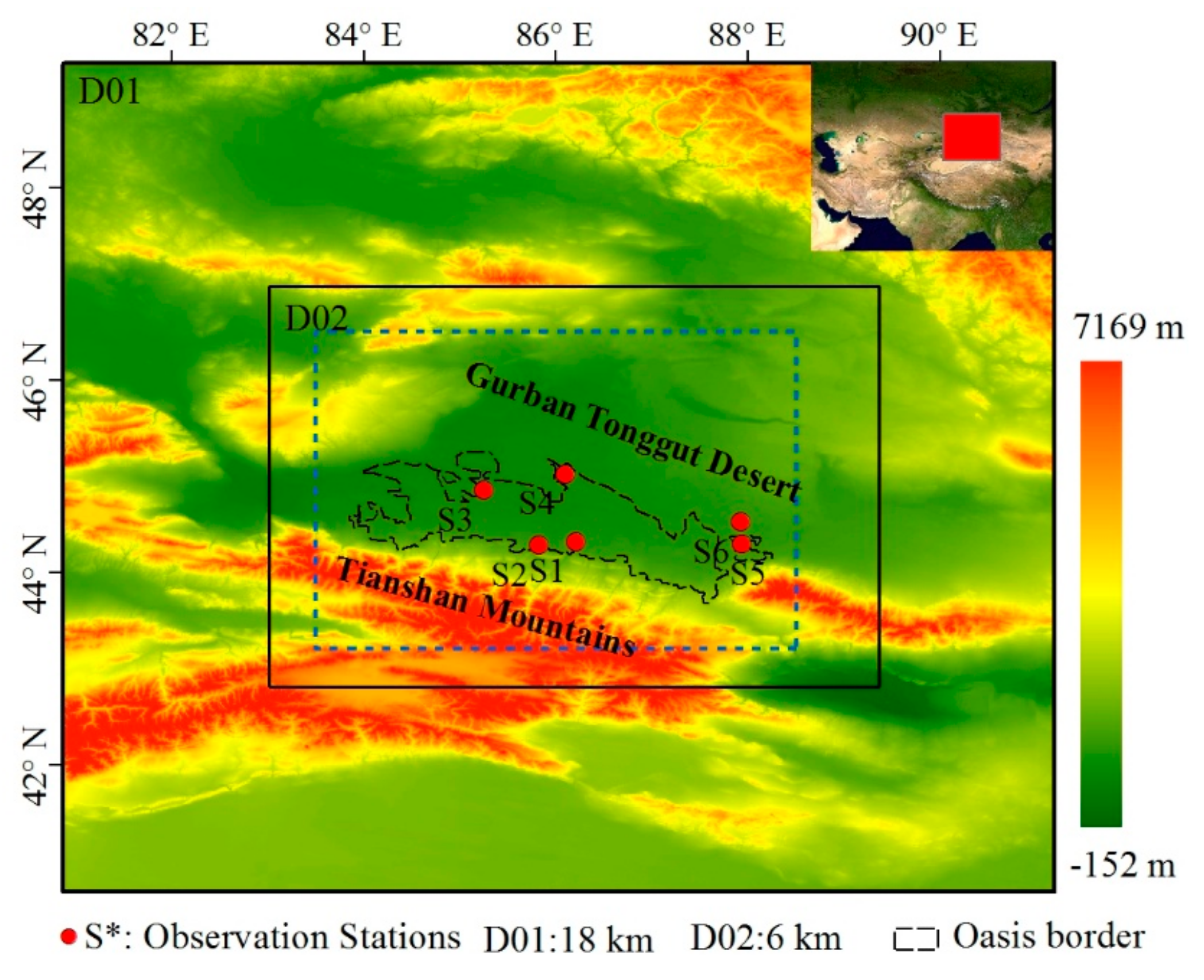
CA is characterized by typical mountain–basin systems. Due to its unique topography, runoff generated from snow- and glacier-melt and precipitation processes [7] in mountainous areas flows into the basin and, by the time these surface waters reach oasis and desert areas, has completely evaporated in the basin. CA is influenced by the westerly circulation at the middle–high latitudes and the polar air masses [7], and experiences an arid continental climate with scarce and concentrated rainfall (less than 250 mm in the basin regions and 900 mm in the mountains). The NTM is representative of the microcosm of the terrain and climate of CA and it includes the southern part of the Tianshan Mountains and the northern part of the Gurban Tonggut Desert (Figure 1). The oasis area is in the groundwater overflow zone and the surrounding deserts in the basin. Two nested grid systems are used in this study (Figure 1). The coarse outer domain (D01) covers the entire area of the NTM and spans a total area of 890 km × 975 km with a grid spacing of 18 km in both horizontal directions. The inner domain (D02), our main region of interest, covers a total area of 530 km × 465 km with a grid spacing of 6 km (Figure 1).
2.2. Datasets
2.2.1. Forcing Data and In Situ Measurements
The latest global atmospheric reanalysis product, ERA-Interim, provided by the European Centre for Medium-Range Weather Forecasting Reanalysis [45], was used for the initial and lateral boundary conditions for WRF simulations in this study; it was chosen because it matches well with most of the local climate records, especially in the low-lying plain areas [1]. We used geopotential, relative humidity, temperature, and U and V wind component data at 30 pressure levels and surface forcing datasets including 10 m U wind, 10 m V wind, 2 m dewpoint temperature, 2 m temperature, mean sea level pressure, sea surface temperature, sea-ice cover, skin temperature, snow density, snow depth, 4-layer soil temperature, and soil water. The dataset has a spatial resolution of 0.75° × 0.75° and is based on 6 h intervals.
Six meteorological stations were used to validate the simulation results (Table 1). These are distributed across the oasis and the surrounding desert areas (Figure 1). Qualified T2, RH at 2 m, wind speed (WS) and wind direction (WD) at 10 m, and precipitation on an hourly scale were retrieved. In addition, we validated simulations of latent heat flux (LE) over the oases using observations from one eddy covariance system installed at station S2 (no effective observations of sensible heat flux were available because the radiation sensor was damaged). Because no surface energy observations were available for the desert areas, we only validated temperature and relative humidity over the desert areas.
2.2.2. LU
The default LU data included in WRF model are originally from the U.S. Geological Survey (USGS), which classifies LU into 24 categories (Table S2) [42]. A high-resolution LU image was produced for 2012 (2012LU) using visual interpretations based on Landsat images and a 1:1,000,000 scale topographic map. This image was generated by the Xinjiang Institute of Ecology and Geography, Chinese Academy of Sciences [46]. The 2012LU has a spatial resolution of 30 m and adopts a hierarchical classification system with a spatial resolution of 30 m, including 6 categories and 25 subcategories (Table S1). We converted it into the USGS classification system according to the relationships shown in Table S2 (please see the Supplementary Materials).
2.2.3. Albedo Product (MCD43A4)
The MODIS Bidirectional Distribution Reflectance Model (BRDF) 16 Day surface albedo standard products have been validated by comparison to in situ measurements [47,48]. The high-quality primary algorithm for the MODIS standard albedo product (MCD43) has also been shown to produce consistent global quantities over a variety of land surface types and snow-covered conditions [49]. We used the nadir BRDF-adjusted reflectance MCD43A4 (MODIS Terra + Aqua Nadir BRDF-Adjusted Reflectance 16 Day L3 Global 500 m SIN Grid V005), which is computed for each MODIS spectral band (1–7) at the mean solar zenith angle. MCD43A4 images, with the strip numbers h23v04 and h24v04 for 3 July 2010 and the same day in 2012, were downloaded from the MODIS website. We reprocessed them using the same coordinate systems and resolutions via numerical simulations.
2.2.4. LAI Product (MYD15A2)
The MODIS global LAI product has been validated into stage 2 by the Committee on Earth Observation Satellites (CEOS) [50,51], and has been determined to have high continuity and consistency for all biome types. On global and regional scales, earth observation (EO)-based estimates of LAI serve as valuable inputs for climate and hydrologic modelling [52]. In this study, the level 4 MODIS global LAI MYD15A2 (MODIS/Terra + Aqua LAI/FPAR 8 Day L3 Global 1 km SIN Grid V005) was used. The data were downloaded from the website listed in Section 2.2.3 and reprocessed using the same coordinate system and resolution as in the numerical simulation.
2.2.5. VF Data from MODIS Vegetation Indices (VI) (MOD13A2)
Currently, validation to stage 3 has been achieved for MODIS VI data (MOD13), and analyses produced by various airborne and field validation campaigns demonstrate that, over most biomes, MODIS near-nadir satellite VI shows strong agreement with top-of-canopy nadir VI and land surface biophysical properties [53,54]. Using this qualified MODIS Normalized Difference Vegetation Index (NDVI), the VF can be calculated as follows [33,41,55]:
where NDVI denotes the NDVI value for each pixel from the MODIS NDVI; NDVIS is the NDVI value for a sparsely vegetated or barren vegetation area; and NDVIV is the NDVI value corresponding to a full vegetation cover type. Both NDVIV and NDVIS are constant, allowing the pixel-level VF to reach theoretical values of 0.0 to 1.0 for any LU. Previous studies [56,57,58,59] have empirically determined NDVIS and NDVIV values of 0.05 and 0.87, respectively. These two parameters serve as global bounds to ensure that the derived VFs vary from 0.0 to 1.0 (i.e., VF = 1.0 when NDVI > 0.87 and VF = 0.0 when NDVI < 0.05 in Equation (1)). The MOD13A2 [60] Version 6 product (MODIS/Terra VI 16 Day L3 Global 1 km Grid SIN V006) was downloaded from the MODIS website [60].
2.3. Model Configuration and Experimental Design
WRF is an advanced mesoscale numerical weather prediction system designed for both atmospheric research and operational forecasting needs. It is jointly administered by the National Center for Atmospheric Research and the National Centers for Environmental Prediction. In this study, simulations used WRF version 3.6 coupled with the Noah land surface model.
WRF was configured for fine-scale simulation with two nested domains (D01 and D02 in Figure 1). In the vertical direction, 35 unevenly spaced full eta levels were defined, and the model top was fixed at 50 hPa. The WRF model was forced by ERA-Interim reanalysis data and was updated every 6 h. Qiu et al. [44] performed a series of analyses examining the model’s sensitivity to different parameterizations of the physical atmospheric processes operating over the study region. In this study, we used the optimal WRF configuration. Planetary boundary layer processes were resolved with the Yonsei University (YSU) scheme [61], microphysics were elucidated via WRF Single Moment-3 (WSM3) [62], cumulus clouds were simulated using the Kain–Fritsch Scheme [63], and the Community Atmospheric Model (CAM) scheme was used to calculate longwave and shortwave radiation [64].
We designed five sets of numerical experiments to investigate using the impact of each of actual LU, albedo, LAI, and VF on model results for 2010 and 2012. The experiments were as follows: the def simulation used default LU, albedo, LAI, and VF provided by the WRF itself; the LU simulation using only actual 2012LU [46]; the Alb simulation used actual LU and albedo datasets; the LAI simulation used actual LU, albedo, and LAI datasets; and the VF simulation used all of actual LU, albedo, LAI, and VF data. The model simulation was initialized from 00:00 UTC on 1 July to 18:00 UTC on 31 July in each year. During this period, the interaction of water and energy between oases and deserts are often the strongest, and oasis crops are at their growth peak. The simulation results were stored hourly with a 60 s time step for integration. Generally, in the absence of accurate, gridded initial soil moisture conditions, a spin-up period is needed to allow the soil moisture within Noah to approach equilibrium within the hydrological cycle [36]. The optimal spin-up period for any particular application is uncertain and may require years to reach equilibrium [65]. In this study, the soil moisture values of oasis and desert areas were initialized via interpolation from observed soil moisture data from similar oasis and desert regions referenced in a previous paper [42] (Table 2). In addition, following previous simulations that were similar for mesoscale water, surface energy, and circulation [14,66,67], the simulation results for the first 21 days were discarded as spin-up, and only simulations for 19:00 UTC on 22 July to 18:00 UTC on 31 July were used for the analysis. According to observation and simulations, 22–31 July were with anticyclonic and clear-sky conditions (Figure S1); thus, the effects of cloud distribution on results were excluded.
3. Results
3.1. Differences between Actual Terrestrial Datasets and the Default Datasets
We first examined the differences between the actual LU, albedo, LAI, and VF data and the corresponding default datasets one by one. Both the defaults and the actual satellite images showed generally correct land surface information for MODS. However, there were significant differences, especially in oasis and desert areas, that were strongly impacted by human activities.
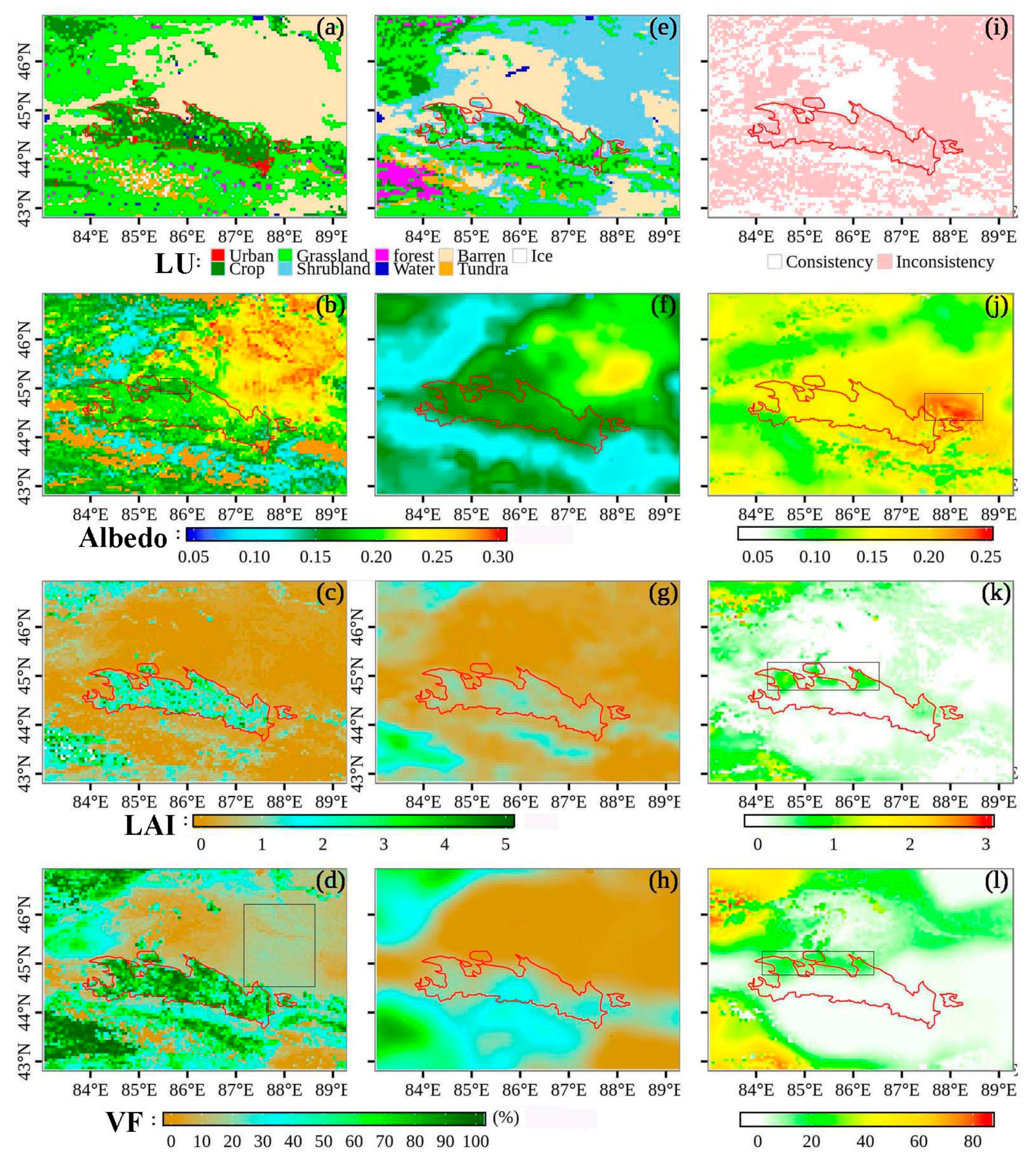
Large areas of cropland and barren desert in oases and north-eastern desert areas are apparent in the actual LU data (Figure 2a), while the default data show grassland and shrubland in these oases and desert areas. The default LU data in WRF is based on AVHRR satellite data for 1992–1993 [42], which represents the original oasis and desert land cover. There has been a large expansion in urban areas and irrigated cropland in the NTM at the expense of sparse shrubland during the last 20 years [68]. In addition, the default LU data shows a large area of forest in the Ili River basin and did not indicate that ice was found on the mountaintops. These areas are misclassified, because dense grassland and cultivated lands have accounted for the largest areal proportion in this river basin over the past 40 years [69], and glaciers are common at the mountaintops in CA. The spatial consistency was only 38.42% between the actual and default LU data using a rough pixel-by-pixel comparison (Figure 2i) [70].
The default albedo, LAI, and VF are based on inter-annual averages of monthly climatology for 1986–1991 [71]. Figure 2b,f,j respectively show the spatial distributions of the actual and default albedo data and the difference between the two. The actual albedo level is overall higher than the default data, ranging from 0.05–0.25 (Figure 2j); the difference between the two datasets mainly occurs in the oasis areas and the northern desert areas (Figure 2b, black rectangle). There is also a slight difference in the values of approximately 0.10 occurring at mountaintops. It is difficult to explain why albedo would be greater in the actual image than in the default dataset; we would expect albedo to decrease with an increase in crop cover. Albedo is influenced by multiple factors, including LU, VF, dynamic roughness lengths, solar elevation angle, soil color, and humidity [72]. The difference in albedo in the oasis area could be related to the severe salinization caused by irrigation [73,74] as well as the expansion of plastic-mulched areas [75] over the past 20 years. The greater albedo in the northern desert area (black rectangle) in Figure 2j can be attributed to the degradation of the desert flora following drawdown of groundwater levels in the oasis–desert transition zone [23,24], which implies that land reclamation and groundwater extraction have led to serious ecological problems in CA oases. In addition, the albedo over crops in the actual image is higher than over the surrounding northern desert area (black rectangle in Figure 2b), but this is not the case for the default data. This indirectly confirms our speculation that oasis salinization and larger areas with plastic mulching could increase the actual albedo levels. The possible reason for slight differences at the mountaintops between the actual and default albedo is that the surface reflectance estimation from different satellite images has large uncertainties over rugged terrain [42,76,77,78,79,80]. The spatial distributions of the actual versus default LAI and VF data, as well as the differences between them, are shown in Figure 2c,d,g,h,k,l, respectively. The differences between actual LAI and VF data and the corresponding default data range from 0 to 3 and from 0 to 85%, respectively. Major differences are evident across the basin, especially near the Ili River basin and the northern oasis border (black rectangle in Figure 2k,l), consistent with the expanded oasis region. There are few differences in the desert and mountainous areas between the actual and default LAI data. In contrast, there are noticeable differences between the actual and default VF data in the desert area, indicating that the default data do not realistically represent VF conditions in this region. Field verification shows that there are sparse desert plants (e.g., Haloxylon and Tamarix ramosissima) with a coverage of approximately 20%. The differences between the actual and default terrestrial datasets confirm that the default datasets are outdated and are less representative of land surface information.
3.2. Validation and Impacts of Actual LU, Albedo, LAI, and VF Data on Atmospheric Modelling
The validation of simulated results is one focus of this paper. We use several statistical measures, including the mean bias error (MBE), root mean squared error (RMSE) and coefficient of determination (R2), to comprehensively evaluate the simulation results [81]. These measures describe the direction of the error bias, and indicate the average error magnitude. We also assess spatial patterns of temperature, humidity, energy, and circulation and determine the difference in their daytime and night-time values by averaging daytime simulations from 19:00 to 2:00 UTC and nocturnal simulations from 08:00 to 14:00 UTC.
3.2.1. Radiation and Surface Energy Fluxes
Figure 3 shows the WRF performance in simulating LE from five simulations over cropland at S2 in 2010 and 2012. The daily average LE from five simulations correctly reproduces the overall shape of the observations (Figure 3a,c), and a strong linear relationship is obtained from all of simulations with coefficients of determination (R2) larger than 0.73 (p < 0.05) (Figure 3b,d). The difference between the five simulations and observations mainly occurs during daytime from 17:00 to 6:00 UTC. The observed daily average maximum value in LE is 244.67 W/m2 in 2010, while the peak values of LE from the def, LU, Alb, LAI, and VF simulations are 158.78 W/m2, 161.81 W/m2, 150.63 W/m2, 176.70 W/m2, and 355.06 W/m2, respectively (Figure 3a). In 2012, the daily average maximum value of LE from observation and the def, LU, Alb, LAI, and VF simulations are 371.50 W/m2, 192.50 W/m2, 191.51 W/m2, 182.74 W/m2, 211.46 W/m2, and 427.27 W/m2, respectively (Figure 3c). The VF simulation slightly overestimates LE and the other four simulations underestimate LE during the daytime in both of the two years. However, the RMSE value of the simulations decreases and R2 increases in the following order: def, LU, Alb, LAI, and VF simulations. The R2 increased from 0.73 to 0.74 in 2010 (Figure 3b) and from 0.92 to 0.94 in 2012 (Figure 3d). The RMSE reduced from 75.81 to 69.05 W/m2 in 2010 (Figure 3b) and from 87.64 to 53.52 W/m2 in 2012 (Figure 3d). These results indicate that the performance of WRF is improved in simulating the surface energy budget by the inclusion of actual LU, albedo, LAI, and VF data in the model. The VF simulation in particular shows considerable improvements in both years; the daily maximum LE value has a much closer resemblance to observations after approximately 1:00 UTC. The VF simulation may have overestimated LE because plastic mulching resulted in lower evaporation [82,83]. This process is not considered in the simulations [14,42].
Using the actual LU, albedo, LAI, and VF datasets during the night-time results in similar spatial patterns of average sensible heat (H) flux. Thus, Figure 4 and Figure 5 only show the daytime spatial patterns of average H and LE from the def, LU, Alb, LAI, and VF simulations and the differences of H and LE resulting from using each of the actual LU, albedo, LAI, and VF datasets. The VF simulation (Figure 4 and Figure 5e) indicates an obvious difference in spatial patterns of H and LE in the basin, compared with that from the other four simulations (Figure 4 and Figure 5a–d). Since evident differences with values of 0–85% are across the Ili River basin and the oases areas between the actual and default VF (Figure 2l), the VF simulation considerably decreases simulation of H by a value of approximately 50–150 W/m2 (Figure 4i) and considerably increases LE by approximately 90–270 W/m2 (Figure 5i) over these areas. Although the def, LU, Alb, and LAI simulations present relatively similar overall spatial patterns of H and LE, some detailed differences have to be noted. Since there is no urban representation in the default LU (Figure 2e), the value of H (LE) is obviously underestimated (overestimated) by approximately 100–150 W/m2 (Figure 4 and Figure 5f) over corresponding grids in the def simulation. Since the default LU data includes a large area of shrubland over the oasis region, and forest in the Ili River valley rather than cropland in the actual LU data, the misclassification results in the def simulation overestimating (underestimating) LE (H) by approximately 50 W/m2 over the corresponding grids (Figure 4 and Figure 5f). In addition, since there is no ice found in the default LU compared with the actual LU, the def simulation overestimates (underestimates) H (LE) in the corresponding areas. These results indicate that the outdated default LU results in an incorrect energy response, especially over the oasis area, the Ili River valley basin, and the glacier region. Realistic representation of LU is important for energy budget simulation, since it determines secondary parameters such as LAI, albedo, emissivity, and surface roughness length. Given that the actual albedo values are slightly greater than the default values, ranging from 0.05–0.25 (Figure 2j), this decreases H and LE in the Alb simulation compared with the LU simulation (Figure 4 and Figure 5c), especially in mountainous areas. Slight differences in H and LE result from using the actual LAI data, with the most obvious differences in the Ili River basin and the northern oasis border (black rectangle in Figure 2k,l).
3.2.2. Air Temperature, Humidity at 2 m
Figure 6 and Figure 7 show aspects of the WRF performance in simulating T2 and RH, respectively, from the five simulations. All of the def, LU, Alb, LAI, and VF simulations reproduce the shape and peak of T2 and RH, and produce a strong linear relationship of T2 and a relatively moderate relationship of RH with the observations at six stations in the two years. The R2 of T2 ranges between 0.71 and 0.95 (p < 0.05), and that of RH ranges between 0.44 and 0.75 (p < 0.05) obtained from all of the five simulations. Although the T2 (RH) from all of the simulations, compared with the observations, is overestimated (underestimated) over both cropland sites (S1, S2, S3, and S4) and over desert sites (S5 and S6) throughout all times of the day, a stronger relationship (increasing R2 progressively) and similar magnitudes of T2 and RH (decreasing RMSE progressively) are observed when each of actual LU, albedo, LAI, and VF datasets was used in the simulations. In particular, at S2, S3, and S4, the bias of temperature was corrected by up to 0.35–2.25 °C and that of relative humidity was corrected by up to 8.85%. Thus, using actual terrestrial datasets improves the WRF performance.
Note that the improvements are relatively smaller at station S1 compared with those at stations S2, S3, and S4. This can be attributed to the fact that the S1 station is located in an urban area, so using actual vegetation parameters such as the LAI or VF does not affect the performance of the WRF model in these areas. The overestimations of T2 and underestimations of RH over oasis areas could be attributed to the cooling or wetting effects of soil evaporation from irrigation; these cannot be simulated by lake irrigation schemes in WRF. All five simulations (the def, LU, Alb, LAI, and VF) captured the rain event that occurred on 28 July 2012 at S1, S3, and S4 (not shown). However, it is difficult to determine whether the use of actual LU, albedo, LAI, and VF data improved the simulation of precipitation due to the limited statistics.
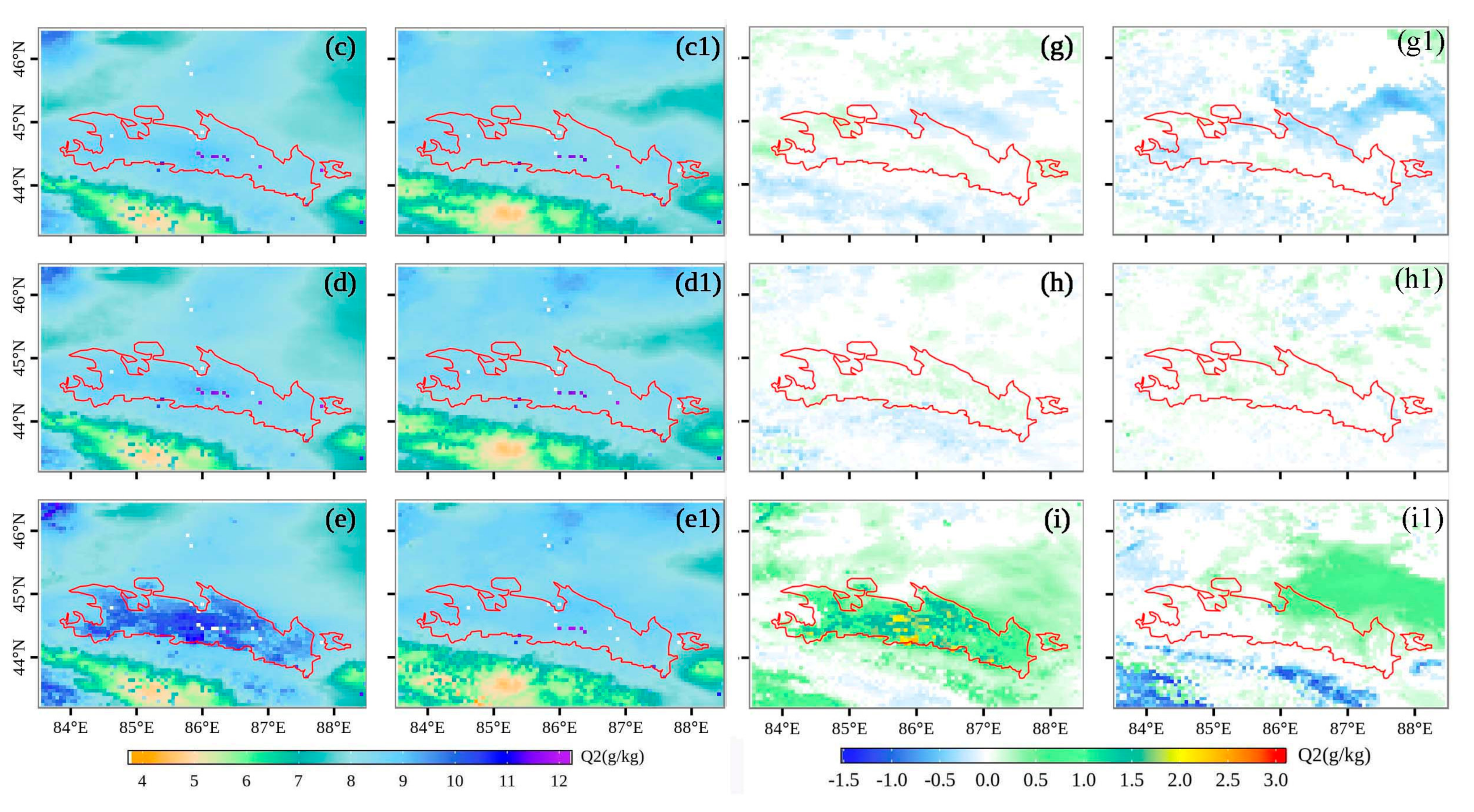
Figure 8 and Figure 9 present spatial patterns of T2 and Q2 from the def, LU, Alb, LAI, and VF simulations, and their differences (the differences of pixels are statistically significant at p < 0.05) using each of actual LU, albedo, LAI, and VF data, respectively. Overall, all of the simulations (the def, LU, Alb, LAI, and VF) generally suggest continuous stripelike T2 increases from the mountainous areas to the basin due to the lapse rate of temperature resulting from the elevation gradient difference. In addition, the simulations show lower Q2 in the mountainous regions as compared to basin areas due to the large difference of temperature in each. Focusing on the difference between oases and desert regions, in accordance with spatial patterns of H and LE, the spatial patterns of T2 and Q2 from the def (Figure 8 and Figure 9a,a1) and VF (Figure 8 and Figure 9e,e1) simulations differ from the LU, Alb, and LAI simulations during the daytime (Figure 8 and Figure 9b–d) and night-time (Figure 8 and Figure 9b1–d1).
Specifically, as indicated by the difference of T2 and Q2 between the LU and def simulations (Figure 8 and Figure 9f,f1), the averaged T2 differences over the oasis area and Ili River valley from the LU simulation decrease up to approximately −0.5 °C in the daytime (Figure 8f) and −1.2 °C at night-time (Figure 8f1), and the averaged Q2 over these areas increases (decreases) 0.25 g kg−1 during the daytime (in night-time) when actual LU data is used in the WRF model (Figure 9f,f1). The differences most likely result from the fact that the default LU over these areas includes sparse shrubland and forest, while the actual LU data show cropland. Since the default LU data do not include urban areas or ice (Figure 2b), there are also large differences in T2 and Q2 over these grids. In addition, there are also obvious differences in T2 and Q2 in the northeast desert when actual LU data was used. Although the LU, Alb, and LAI simulations can simulate the cold–wet island effects of the area during the daytime, this effect is more intense in the VF simulation than in the other three simulations. Using actual VF data results in a significant decrease in T2 of −0.5 to −1.5 °C during the day (Figure 8i) and −0.5 to −4.5 °C (Figure 8i1) at night; similarly, there is a large increase in Q2 by 0.5–2.5 g kg−1 during the day (Figure 9i) and a decrease of 1.0 g kg−1 at night (Figure 9i1) over the oasis area and Ili River Valley. Using actual albedo data results in a slight decrease in T2 of approximately −0.45 °C (Figure 8g1) and a decrease in Q2 of approximately 0.5 g kg−1 (Figure 9g1) over the north-eastern desert at night, as shown by the difference between the Alb and LU simulations. Using actual LAI data results in a slight decrease in T2 by approximately −0.15 °C (Figure 8h,h1), and an increase in Q2 by approximately 0.25 g kg−1 over the oasis region for the whole day (Figure 9h,h1). Overall, actual LU and VF data strongly influence the simulations of T2 and Q2 patterns in the oasis–desert system, while albedo and LAI have a lesser impact.
3.2.3. Surface Circulation
Figure 10 shows comparisons of the simulated 10 m horizontal WS and WD from the def, LU, Alb, LAI, and VF simulations with observations at three meteorological stations over cropland. Station S1 is located in the upper part of the oasis, near its southern border, and stations S3 and S4 are located in the lower part of the oasis, near its northern border. Although the RMSE (R2) of the WS decreases slightly (increases) as actual data are added in the def, LU, Alb, LAI, and VF simulations, most of the simulated WS values are higher than the observed values by approximately 2 m/s; 60% of the simulated WS range from 2–6 m/s, whereas the observed values range from 2–4 m/s. The reason for this bias in WS is that the uncertainty of randomized turbulence processes results in difficulties in the accurate simulation of wind patterns [84]. The trends in WD are consistent with the observations. The dominant WD is WNW or NW during the daytime and WSW or SW during the night-time for all stations; these directions are observed in all simulations and in the observations, and reflect the circulation characteristics in a mountain–valley region.
Figure 11 shows the WS and WD patterns from the def, LU, Alb, LAI, and VF simulations and the differences caused by using each of the actual LU, albedo, LAI, and VF datasets. Overall, the simulations (def, LU, Alb, LAI, and VF) reflect the characteristics of mountain–valley winds, which have WDs to the WNW or NW during the day and to the WSW or SW at night. Using actual LU, albedo, and LAI data has very little impact on the spatial patterns of WD (Figure 11f–h1), but using actual VF data causes slight differences in the oasis center and the surrounding desert (Figure 11i,i1). These results suggest that using actual VF data increases the intensity of oasis effects (cold–wet island effects, and OBC).
3.2.4. Impacts of Using Actual Datasets on Atmospheric Modelling
To quantitatively discern which terrestrial datasets have the strongest influence on the meteorological elements simulated in this region, the bias percentage was calculated as the general regional influence index, following the approach in [85]. After land surface parameters are replaced, the equation is as follows:
In the current study, n is the number of stations, is the simulated meteorological variables (e.g., temperature) with updated actual land surface parameters from experiment j, and is the observed value at each station. Four modelled predictors (T2, RH, WS, and LE) are analyzed.
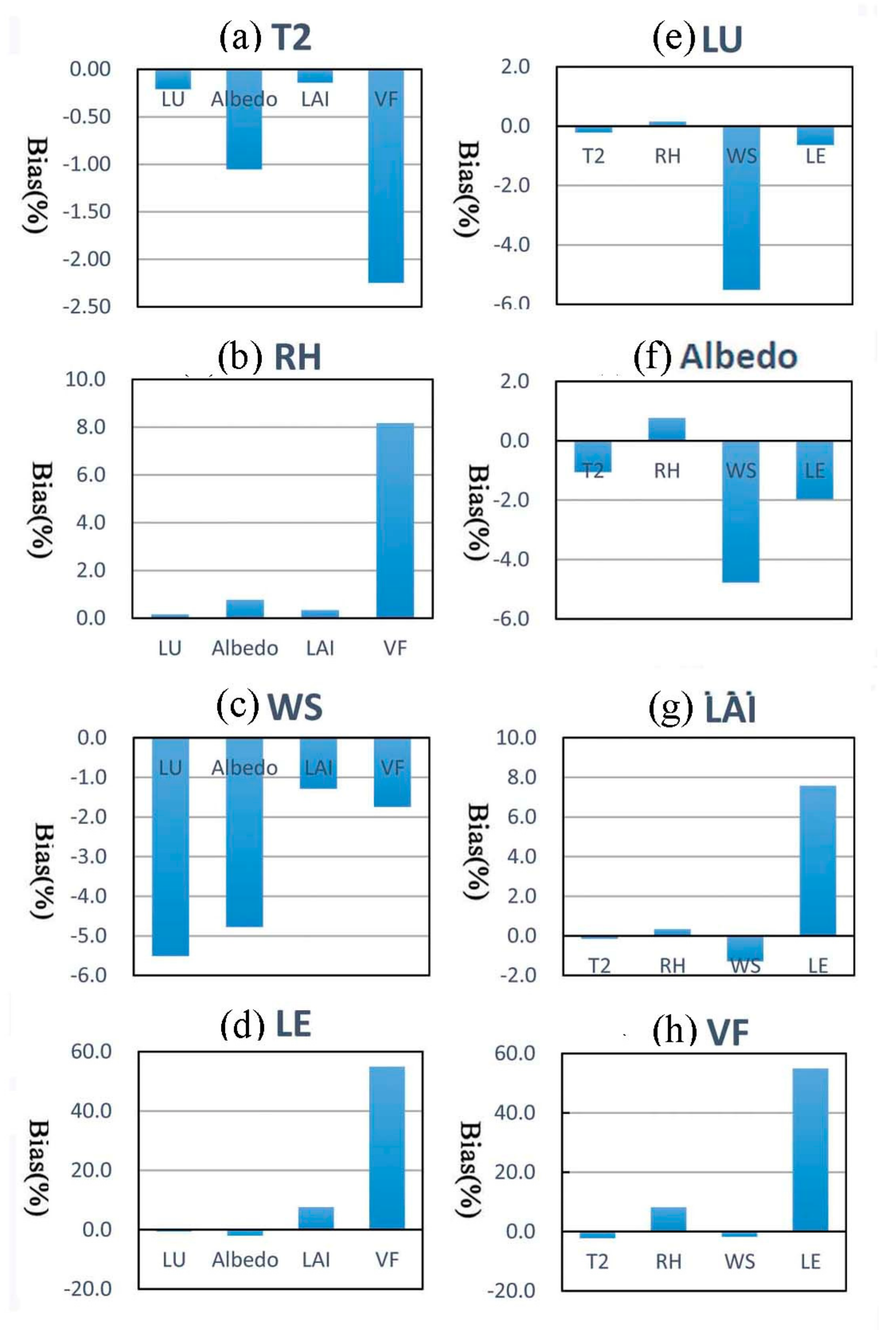
Figure 12 presents the bias percentage of the simulated T2, RH, WS, and LE due to using each actual dataset. The y axis shows the mean bias percentage for 2010 and 2012, which represents the impact of using each actual dataset on atmospheric simulations. Using actual LAI and VF data mainly affects the LE (Figure 12g,h), while using actual LU and albedo data affects the WS (Figure 12c,f). T2 (RH) decreases (increases) by a total of −3.5% (10.2%) from using actual LU, albedo, LAI, and VF data. In total, −2.26% (8.85%) of the change in T2 (RH) is contributed by using actual VF data, and the remainder comes from using actual data for albedo and the other two parameters (Figure 12a,b). The WS decreases by −13.31% when actual LU, albedo, LAI, and VF data are used; of that total, LU and albedo contribute −5.51% and −4.47%, respectively—far more than the other two parameters (Figure 12c). The LE first decreases due to the use of actual LU and albedo data and then increases with the addition of actual LAI and VF data; the total change is 58.19%, of which VF contributes 54.94%, which is far more than the other three parameters (Figure 12d). In general, using actual land surface parameters alters the near-surface meteorology simulation in the lower atmospheric layer (Figure 12e–h). Using actual VF data has a large influence on the simulation of T2, RH, and LE in the oasis–desert system, which contributes to error correction values of 62%, 87%, and 92%. Thus, using actual VF data is very important for simulating near-surface meteorology. Using actual LU is the principal parameter for near-surface water and heat simulation, since it determines the value of secondary parameters such as LAI, albedo, emissivity, and surface roughness length.
4. Discussion
Outdated default terrestrial datasets in WRF, including LU, albedo, LAI, and VF, limit this model’s ability to accurately simulate the meteorological characteristics of the complex oasis–desert system in NTM. In this study, we examined the impact of using actual LU, albedo, LAI, and VF data from satellite products in WRF on the model performance. Five simulations were conducted with the same meteorological forcing data and model schemes: def (using default LU, albedo, LAI, and VF data), LU (using actual LU data only), Alb (using actual LU and albedo data only), LAI (using actual LU, albedo, and LAI), and VF (using all of actual LU, albedo, LAI, and VF together).
WRF simulations of temperature, humidity, energy, and WS are improved by the incorporation of actual LU, albedo, LAI, and VF into the model, as evidenced by the decrease in RMSE values and increase in R2 in both 2010 and 2012. Using actual VF data greatly affects the simulation of T2, RH, and LE in the oasis–desert system, contributing to error correction values of 62%, 87%, and 92%, respectively. LU data is a primary parameter and it determines the values of many secondary parameters. Although all of the simulations conducted in this study produce the characteristic of the “wet–cold” island effect over the oasis area, as reported previously [7,14,71,72], WRF can more accurately reflect the intensity of the oasis cold–wet effects when using all actual LU, albedo, LAI, and VF data. The results of this study contribute to a greater knowledge of the impacts of land surface parameters on the performance of WRF [42], which is beneficial for various applications, especially for land surface and climate modelling. Our results are also critical to accurately understanding the intensity of cold–wet effects of oases and the OBC.
We note that our simulations have several limitations. For example, overall, we found that the simulations overestimated (underestimated) T2 (RH), and the VF simulation overestimates the LE relative to the observations. These errors can be attributed to the fact that soil evaporation resulting from irrigation and plastic mulching effects are not considered in the simulations of WRF [14,42]. Adding irrigation and plastic mulching schemes may help to correct these errors.
5. Conclusions
The current study used WRF with actual LU, albedo, LAI, and VF data derived from satellite products to improve the simulation of weather and climate conditions in the oasis–desert system of the NTM in 2010 and 2012. Model evaluations for temperature, humidity, and energy demonstrated that our simulations, which were performed using actual terrestrial datasets, improved the performance of WRF, as evidenced by the decrease in RMSE and the increase in R2. All of the simulations exhibit the “wet–cold” island effects of the oases. However, the intensity of the wet–cold effect varies depending on the use of actual LU, albedo, LAI, and VF data. Using actual VF data results in error correction values of 62%, 87%, and 92%, respectively, for simulated T2, RH, and LE in the oasis–desert system. Using actual LU data is crucial for near-surface water and heat simulation, since it determines the values of additional secondary parameters. We conclude that it is important to use, at least, actual LU and VF data for weather and climate simulations in WRF.
Supplementary Materials
The following are available online at www.mdpi.com/2072-4292/9/12/1273/s1, Table S1: Shows LU types and codes of for the 2012LU; Table S2: Land use type and its categories for WRF and the 2012LU.
Acknowledgments
This work was supported financially by the International Partnership Program of the Chinese Academy of Science (Grant No. 131965KYSB20160004) and the National Natural Science Foundation of China (Grant No. U1303382, 41671108). The authors declare no conflicts of interest.
Author Contributions
Miao Zhang and Geping Luo conceived and designed the experiments; Miao Zhang and Peng Cai performed the experiments and analyzed the data; and Miao Zhang, Philippe De Maeyer and Alishir Kurban jointly revised the paper.
Conflicts of Interest
The authors declare no conflict of interest.
Abbreviations
| AVHRR | Advanced Very High Resolution Radiometer |
| BRDF | Bidirectional reflectance distribution function |
| CA | Central Asia |
| LAI | Leaf area index |
| LE | Latent heat flux |
| LU | Land use |
| MBE | Mean bias error |
| MM5 | Fifth-generation Penn State/NCAR Mesoscale Model |
| MODIS | MODerate Resolution Imaging Spectroradiometer |
| NCAR | National Center for Atmospheric Research |
| NCEP | National Centers for Environmental Prediction |
| NTM | North Tianshan Mountains |
| OBC | Oasis breeze circulation |
| Q2 | Specific humidity at 2 m |
| R2 | Coefficient of determination |
| RMSE | Root mean squared error |
| RH | 2-m relative humidity |
| RCMs | Regional climate models |
| T2 | 2-m air temperature |
| TIL | Temperature inversion layer |
| USGS | U.S. Geological Survey |
| VF | Vegetation fraction |
| WRF | Weather Research and Forecasting model |
| WS | Wind speed |
| WD | Wind direction |
References
- Hu, Z.; Zhang, C.; Hu, Q.; Tian, H. Temperature changes in central asia from 1979 to 2011 based on multiple datasets. J. Clim. 2014, 27, 1143–1167. [Google Scholar] [CrossRef]
- Li, C.F.; Zhang, C.; Luo, G.P.; Chen, X.; Maisupova, B.; Madaminov, A.A.; Han, Q.F.; Djenbaev, B.M. Carbon stock and its responses to climate change in central Asia. Glob. Chang. Biol. 2015, 21, 1951–1967. [Google Scholar] [CrossRef] [PubMed]
- Zhang, B.; Tan, Y.; Mo, K.G. Digital spectrum and analysis of altitudinal belts in the tianshan mountains. Mt. Res. 2004, 22, 8. [Google Scholar]
- Gessner, U.; Naeimi, V.; Klein, I.; Kuenzer, C.; Klein, D.; Dech, S. The relationship between precipitation anomalies and satellite-derived vegetation activity in central Asia. Glob. Planet. Chang. 2013, 110, 74–87. [Google Scholar] [CrossRef]
- Immerzeel, W.W.; Van Beek, L.P.; Bierkens, M.F. Climate change will affect the asian water towers. Science 2010, 328, 1382–1385. [Google Scholar] [CrossRef] [PubMed]
- Luo, G.P.; Feng, Y.X.; Zhang, B.P.; Cheng, W.M. Sustainable land-use patterns for arid lands: A case study in the northern slope areas of the Tianshan Mountains. J. Geogr. Sci. 2010, 20, 510–524. [Google Scholar] [CrossRef]
- Bothe, O.; Fraedrich, K.; Zhu, X.H. Precipitation climate of central asia and the large-scale atmospheric circulation. Theor. Appl. Climatol. 2012, 108, 345–354. [Google Scholar] [CrossRef]
- Deng, M.J. Current situation and its potential analysis of exploration and utilization of groundwater resources of Xinjiang. Arid Land Geogr. 2009, 32, 647–654. [Google Scholar]
- Souza, V.; Espinosa-Asuar, L.; Escalante, A.E.; Eguiarte, L.E.; Farmer, J.; Forney, L.; Lloret, L.; Rodríguez-Martínez, J.M.; Soberón, X.; Dirzo, R. An endangered oasis of aquatic microbial biodiversity in the chihuahuan desert. Proc. Natl. Acad. Sci. USA 2006, 103, 6565–6570. [Google Scholar] [CrossRef] [PubMed]
- Smith, J.R.; Hawkins, A.L.; Asmerom, Y.; Polyak, V.; Giegengack, R. New age constraints on the middle stone age occupations of kharga oasis, Western Desert, Egypt. J. Hum. Evol. 2007, 52, 690–701. [Google Scholar] [CrossRef] [PubMed]
- Soltan, M. Evaluation of ground water quality in dakhla oasis (Egyptian Western Desert). Environ. Monit. Assess. 1999, 57, 157–168. [Google Scholar] [CrossRef]
- Li, J.; Zhao, C.; Zhu, H.; Li, Y.; Wang, F. Effect of plant species on shrub fertile island at an oasis–desert ecotone in the south junggar basin, China. J. Arid Environ. 2007, 71, 350–361. [Google Scholar] [CrossRef]
- Liu, S.H.; Liu, H.P.; Hu, Y.; Zhang, C.; Liang, F.; Wang, J. Numerical simulations of land surface physical processes and land-atmosphere interactions over oasis-desert/gobi region. Sci. China Ser. D Earth Sci. 2007, 50, 290–295. [Google Scholar] [CrossRef]
- Meng, X.H.; Lü, S.H.; Zhang, T.T.; Guo, J.X.; Gao, Y.H.; Bao, Y.; Wen, L.J.; Luo, S.Q.; Liu, Y.P. Numerical simulations of the atmospheric and land conditions over the jinta oasis in northwestern China with satellite-derived land surface parameters. Int. J. Climatol. 2009, 114. [Google Scholar] [CrossRef]
- Sorg, A.; Bolch, T.; Stoffel, M.; Solomina, O.; Beniston, M. Climate change impacts on glaciers and runoff in tien shan (central Asia). Nat. Clim. Chang. 2012, 2, 725–731. [Google Scholar] [CrossRef]
- He, Q.; Yang, Q.; Li, H.-J. Variations of air temperature, precipitation and sand-dust weather in Xinjiang in past 40 years. J. Glaciol. Geocryol. 2003, 25, 423–427. [Google Scholar]
- Xu, G.-Q.; Wei, W.-S. Climate change of Xinjiang and its impact on eco-enviroment. Arid Land Geogr. 2004, 1, 14–27. [Google Scholar]
- Lianmei, Y. Climate change of extreme precipitation in Xinjiang. Acta Geogr. Sin. 2003, 58, 577–583. [Google Scholar]
- Lioubimtseva, E.; Henebry, G.M. Climate and environmental change in arid central asia: Impacts, vulnerability, and adaptations. J. Arid Environ. 2009, 73, 963–977. [Google Scholar] [CrossRef]
- Zhang, H.; Wu, J.-W.; Zheng, Q.-H.; Yu, Y.-J. A preliminary study of oasis evolution in the tarim basin, Xinjiang, China. J. Arid Environ. 2003, 55, 545–553. [Google Scholar]
- Zhang, Q.; Luo, G.; Li, L.; Zhang, M.; Lv, N.; Wang, X. An analysis of oasis evolution based on land use and land cover change: A case study in the sangong river basin on the northern slope of the Tianshan Mountains. J. Geogr. Sci. 2017, 27, 223–239. [Google Scholar] [CrossRef]
- Jia, B.; Zhang, Z.; Ci, L.; Ren, Y.; Pan, B.; Zhang, Z. Oasis land-use dynamics and its influence on the oasis environment in Xinjiang, China. J. Arid Environ. 2004, 56, 11–26. [Google Scholar] [CrossRef]
- Sun, D.; Zhao, C.; Wei, H.; Peng, D. Simulation of the relationship between land use and groundwater level in tailan river basin, Xinjiang, China. Quat. Int. 2011, 244, 254–263. [Google Scholar] [CrossRef]
- Wang, Y.; Xiao, D.; Li, Y.; Li, X. Soil salinity evolution and its relationship with dynamics of groundwater in the oasis of inland river basins: Case study from the fubei region of Xinjiang Province, China. Environ. Monit. Assess. 2008, 140, 291–302. [Google Scholar] [CrossRef] [PubMed]
- Lioubimtseva, E.; Cole, R.; Adams, J.M.; Kapustin, G. Impacts of climate and land-cover changes in arid lands of central Asia. J. Arid Environ. 2005, 62, 285–308. [Google Scholar] [CrossRef]
- Yao, Y.H.; Zhang, B.P. A preliminary study of the heating effect of the Tibetan Plateau. PLoS ONE 2013, 8. [Google Scholar] [CrossRef] [PubMed]
- Zhou, Y.; Zhang, L.; Fensholt, R.; Wang, K.; Vitkovskaya, I.; Tian, F. Climate contributions to vegetation variations in central asian drylands: Pre-and post-ussr collapse. Remote Sens. 2015, 7, 2449–2470. [Google Scholar] [CrossRef]
- Horton, D.E.; Johnson, N.C.; Singh, D.; Swain, D.L.; Rajaratnam, B.; Diffenbaugh, N.S. Contribution of changes in atmospheric circulation patterns to extreme temperature trends. Nature 2015, 522, 465–469. [Google Scholar] [CrossRef] [PubMed]
- Qu, R.; Cui, X.; Yan, H.; Ma, E.; Zhan, J. Impacts of land cover change on the near-surface temperature in the North China plain. Adv. Meteorol. 2013, 2013, 153–156. [Google Scholar] [CrossRef]
- Yan, J.W.; Liu, J.Y.; Chen, B.Z.; Feng, M.; Fang, S.F.; Xu, G.; Zhang, H.F.; Che, M.L.; Liang, W.; Hu, Y.F. Changes in the land surface energy budget in eastern China over the past three decades: Contributions of land-cover change and climate change. J. Clim. 2014, 27, 9233–9252. [Google Scholar] [CrossRef]
- Yu, G.R.; Wen, X.F.; Sun, X.M.; Tanner, B.D.; Lee, X.H.; Chen, J.Y. Overview of chinaflux and evaluation of its eddy covariance measurement. Agric. For. Meteorol. 2006, 137, 125–137. [Google Scholar] [CrossRef]
- Li, X.; Cheng, G.D.; Liu, S.M.; Xiao, Q.; Ma, M.G.; Jin, R.; Che, T.; Liu, Q.H.; Wang, W.Z.; Qi, Y. Heihe watershed allied telemetry experimental research (hiwater): Scientific objectives and experimental design. Bull. Am. Meteor. Soc. 2013, 94, 1145–1160. [Google Scholar] [CrossRef]
- Seungbum, H.; Lakshmi, V.; Small, E.E.; Chen, F.; Tewari, M.; Manning, K.W. Effects of vegetation and soil moisture on the simulated land surface processes from the coupled WRF/Noah model. Int. J. Climatol. 2009, 114. [Google Scholar] [CrossRef]
- Seneviratne, S.I.; Lüthi, D.; Litschi, M.; Schär, C. Land–atmosphere coupling and climate change in Europe. Nature 2006, 443, 205–209. [Google Scholar] [CrossRef] [PubMed]
- Kyselý, J.; Rulfová, Z.; Farda, A.; Hanel, M. Convective and stratiform precipitation characteristics in an ensemble of regional climate model simulations. Clim. Dyn. 2016, 46, 227–243. [Google Scholar] [CrossRef]
- Branch, O.; Warrach-Sagi, K.; Wulfmeyer, V.; Cohen, S. Simulation of semi-arid biomass plantations and irrigation using the WRF-Noah model—A comparison with observations from israel. Hydrol. Earth Syst. Sci. 2014, 18, 1761–1783. [Google Scholar] [CrossRef]
- Cao, Q.; Yu, D.Y.; Georgescu, M.; Han, Z.; Wu, J.G. Impacts of land use and land cover change on regional climate: A case study in the agro-pastoral transitional zone of China. Environ. Res. Lett. 2015, 10. [Google Scholar] [CrossRef]
- Lenderink, G.; Van Ulden, A.; Van den Hurk, B.; Van Meijgaard, E. Summertime inter-annual temperature variability in an ensemble of regional model simulations: Analysis of the surface energy budget. Clim. Chang. 2007, 81, 233–247. [Google Scholar] [CrossRef]
- Vidale, P.L.; Lüthi, D.; Wegmann, R.; Schär, C. European summer climate variability in a heterogeneous multi-model ensemble. Clim. Chang. 2007, 81, 209–232. [Google Scholar] [CrossRef]
- Deng, X.Z.; Shi, Q.L.; Zhang, Q.; Shi, C.C.; Yin, F. Impacts of land use and land cover changes on surface energy and water balance in the Heihe River basin of China, 2000–2010. Phys. Chem. Earth Parts A/B/C 2015, 79–82, 2–10. [Google Scholar] [CrossRef]
- Yin, J.F.; Zhan, X.W.; Zheng, Y.F.; Hain, C.R.; Ek, M.; Wen, J.; Fang, L.; Liu, J.C. Improving noah land surface model performance using near real time surface albedo and green vegetation fraction. Agric. For. Meteorol. 2016, 218, 171–183. [Google Scholar] [CrossRef]
- Wen, X.H.; Lu, S.H.; Jin, J.M. Integrating remote sensing data with WRF for improved simulations of oasis effects on local weather processes over an arid region in Northwestern China. J. Hydrol. 2012, 13, 573–587. [Google Scholar] [CrossRef]
- Xu, Z.F.; Mahmood, R.; Yang, Z.L.; Fu, C.; Su, H. Investigating diurnal and seasonal climatic response to land use and land cover change over monsoon Asia with the community earth system model. Int. J. Climatol. 2015, 120, 1137–1152. [Google Scholar] [CrossRef]
- Qiu, Y.; Hu, Q.; Zhang, C. WRF simulation and downscaling of local climate in central Asia. Int. J. Climatol. 2017, 37, 513–528. [Google Scholar] [CrossRef]
- Dee, D.P.; Uppala, S.M.; Simmons, A.J.; Berrisford, P.; Poli, P.; Kobayashi, S.; Andrae, U.; Balmaseda, M.A.; Balsamo, G.; Bauer, P. The era-interim reanalysis: Configuration and performance of the data assimilation system. Q. J. R. Meteorol. Soc. 2011, 137, 553–597. [Google Scholar] [CrossRef]
- Chen, X.B. Land Use/Cover Change in Arid Area in China, 1st ed.; China Science Publishing & Media Ltd.: Beijing, China, 2008; pp. 55–124. ISBN 9787030200372. [Google Scholar]
- Cescatti, A.; Marcolla, B.; Vannan, S.K.S.; Pan, J.Y.; Román, M.O.; Yang, X.; Ciais, P.; Cook, R.B.; Law, B.E.; Matteucci, G. Intercomparison of modis albedo retrievals and in situ measurements across the global fluxnet network. Remote Sens. Environ. 2012, 121, 323–334. [Google Scholar] [CrossRef]
- Stroeve, J.; Box, J.E.; Wang, Z.; Schaaf, C.; Barrett, A. Re-evaluation of modis MCD43 greenland albedo accuracy and trends. Remote Sens. Environ. 2013, 138, 199–214. [Google Scholar] [CrossRef]
- Román, M.O.; Gatebe, C.K.; Shuai, Y.; Wang, Z.; Gao, F.; Masek, J.G.; He, T.; Liang, S.; Schaaf, C.B. Use of in situ and airborne multiangle data to assess modis-and landsat-based estimates of directional reflectance and albedo. IEEE Trans. Geosci. Remote Sens. 2013, 51, 1393–1404. [Google Scholar] [CrossRef]
- Yan, K.; Park, T.; Yan, G.; Chen, C.; Yang, B.; Liu, Z.; Nemani, R.R.; Knyazikhin, Y.; Myneni, R.B. Evaluation of modis lai/fpar product collection 6. Part 1: Consistency and improvements. Remote Sens. 2016, 8, 359. [Google Scholar] [CrossRef]
- Yan, K.; Park, T.; Yan, G.j.; Liu, Z.; Yang, B.; Chen, C.; Nemani, R.R.; Knyazikhin, Y.; Myneni, R.B. Evaluation of MODIS LAI/FPAR product collection 6. Part 2: Validation and intercomparison. Remote Sens. 2016, 8, 460. [Google Scholar] [CrossRef]
- Fensholt, R.; Sandholt, I.; Rasmussen, M.S. Evaluation of modis lai, fapar and the relation between fapar and ndvi in a semi-arid environment using in situ measurements. Remote Sens. Environ. 2004, 91, 490–507. [Google Scholar] [CrossRef]
- Sesnie, S.E.; Dickson, B.G.; Rosenstock, S.S.; Rundall, J.M. A comparison of landsat tm and modis vegetation indices for estimating forage phenology in desert bighorn sheep (Ovis canadensis nelsoni) habitat in the sonoran desert, USA. Int. J. Remote Sens. 2012, 33, 276–286. [Google Scholar] [CrossRef]
- Sims, D.A.; Rahman, A.F.; Vermote, E.F.; Jiang, Z. Seasonal and inter-annual variation in view angle effects on modis vegetation indices at three forest sites. Remote Sens. Environ. 2011, 115, 3112–3120. [Google Scholar] [CrossRef]
- Miller, J.; Barlage, M.; Zeng, X.; Wei, H.; Mitchell, K.; Tarpley, D. Sensitivity of the ncep/noah land surface model to the modis green vegetation fraction data set. Geophys. Res. Lett. 2006, 33. [Google Scholar] [CrossRef]
- Zeng, X.B.; Dickinson, R.E.; Walker, A.; Shaikh, M.; DeFries, R.S.; Qi, J. Derivation and evaluation of global 1-km fractional vegetation cover data for land modeling. J. Appl. Meteorol. 2000, 39, 826–839. [Google Scholar] [CrossRef]
- Gutman, G.; Ignatov, A. The derivation of the green vegetation fraction from NOAA/AVHRR data for use in numerical weather prediction models. Int. J. Remote Sens. 1998, 19, 1533–1543. [Google Scholar] [CrossRef]
- Jiang, L.; Kogan, F.N.; Guo, W.; Tarpley, J.D.; Mitchell, K.E.; Ek, M.B.; Tian, Y.; Zheng, W.; Zou, C.Z.; Ramsay, B.H. Real-time weekly global green vegetation fraction derived from advanced very high resolution radiometer-based noaa operational global vegetation index (GVI) system. Int. J. Climatol. 2010, 115. [Google Scholar] [CrossRef]
- Li, X.S.; Zhang, J. Derivation of the green vegetation fraction of the whole China from 2000 to 2010 from modis data. Earth Interact. 2016, 20, 1–16. [Google Scholar] [CrossRef]
- MODIS/Terra Vegetation Indices 16-Day L3 Global 1km Grid SIN V006. Available online: https://lpdaac.usgs.gov/dataset_discovery (accessed on 3 April 2016).
- Song, Y.H.; Noh, Y.; Dudhia, J. A new vertical diffusion package with an explicit treatment of entrainment processes. Mon. Weather Rev. 2006, 134, 2318–2341. [Google Scholar]
- Song, Y.H.; Dudhia, J.; Chen, S.H. A revised approach to ice microphysical processes for the bulk parameterization of clouds and precipitation. Mon. Weather Rev. 2004, 132, 103–120. [Google Scholar]
- Bretherton, C.S.; McCaa, J.R.; Grenier, H. A new parameterization for shallow cumulus convection and its application to marine subtropical cloud-topped boundary layers. Part I: Description and 1D results. Mon. Weather Rev. 2004, 132, 864–882. [Google Scholar] [CrossRef]
- Collins, W.; Rasch, P.; Boville, B.A.; Hack, J.J.; McCaa, J.R.; Williamson, D.L.; Kiehl, J.T.; Briegleb, B.; Bitz, C.; Lin, S.J. Description of the NCAR Community Atmosphere Model (CAM 3.0); Technical Report; National Center for Atmospheric Research: Boulder, CO, USA, 2004. [Google Scholar] [CrossRef]
- Lim, Y.-J.; Hong, J.; Lee, T.-Y. Spin-up behavior of soil moisture content over east asia in a land surface model. Meteor. Atmos. Phys. 2012, 118, 151–161. [Google Scholar] [CrossRef]
- Chu, P.; Liv, S.H.; Chen, Y.C. A numerical modeling study on desert oasis self-supporting mechanisms. J. Hydrol. 2005, 312, 256–276. [Google Scholar] [CrossRef]
- Meng, X.H.; Lu, S.; Zhang, T.; Ao, Y.; Li, S.; Bao, Y.; Wen, L.; Luo, S. Impacts of inhomogeneous landscapes in oasis interior on the oasis self-maintenance mechanism by integrating numerical model with satellite data. Hydrol. Earth Syst. Sci. 2012, 16, 3729–3738. [Google Scholar] [CrossRef] [Green Version]
- Fan, Z.; Wu, S.; Wu, Y.; Zhang, P.; Zhao, X.; Zhang, J. The land reclamation in xinjiang since the founding of new China. J. Nat. Resour. 2013, 28, 713–720. [Google Scholar]
- Zhu, L.; Luo, G.P.; Chen, X.; Xu, W.; Feng, Y.; Zhen, Q.; Wang, J.; Zhou, D.; Yin, C. Detection of land use/land cover change in the middle and lower reaches of the Ili river, 1970–2007. Prog. Geogr. 2010, 29, 292–300. [Google Scholar]
- Zhang, M.; Ma, M.; De Maeyer, P.; Kurban, A. Uncertainties in classification system conversion and an analysis of inconsistencies in global land cover products. ISPRS Int. J. Geo Inf. 2017, 6, 112. [Google Scholar] [CrossRef]
- Kumar, A.; Chen, F.; Barlage, M.; Ek, M.B.; Niyogi, D. Assessing impacts of integrating modis vegetation data in the weather research and forecasting (WRF) model coupled to two different canopy-resistance approaches. J. Appl. Meteorol. 2014, 53, 1362–1380. [Google Scholar] [CrossRef]
- Zhang, C.; Fan, G.; Ma, Z.; Cheng, B.; Zhao, B.; Feng, J.; Wang, H. Characteristics of albedo over different underlying surface in the semi-arid area. Plateau Meteorol. 2015, 34, 1029–1040. [Google Scholar]
- Litan, S.; Shalamu, A.; Yu-dong, S. Effects of drip irrigation volume on soil water-salt transfer and its redistribution. Arid Zone Res. 2011, 1, 79–84. [Google Scholar]
- Zhang, L.; Jiang, P.; Wu, H.; Li, M. Research on spectral characteristics of typical soil in North Xinjiang. J. Soil Water Conserv. 2013, 4, 273–276. [Google Scholar]
- Liu, X.; Tian, C. Study on dynamic and balance of salt for cotton under plastic mulch in South Xinjiang. J. Soil Water Conserv. 2005, 6, 82–85. [Google Scholar]
- Wen, J.; Zhao, X.; Liu, Q.; Tang, Y.; Dou, B. An improved land-surface albedo algorithm with dem in rugged terrain. IEEE Geosci. Remote Sens. Lett. 2014, 11, 883–887. [Google Scholar]
- Wen, J.; Dou, B.; You, D.; Tang, Y.; Xiao, Q.; Liu, Q.; Qinhuo, L. Forward a small-timescale BRDF/Albedo by multisensor combined brdf inversion model. IEEE Trans. Geosci. Remote Sens. 2017, 55, 683–697. [Google Scholar] [CrossRef]
- Wen, J.; Liu, Q.; Tang, Y.; Dou, B.; You, D.; Xiao, Q.; Liu, Q.; Li, X. Modeling land surface reflectance coupled brdf for HJ-1/CCD data of rugged terrain in Heihe River basin, China. IEEE J. Sel. Top. Appl. Earth Obs. Remote Sens. 2015, 8, 1506–1518. [Google Scholar] [CrossRef]
- Wen, J.; Liu, Q.; Liu, Q.; Xiao, Q.; Li, X. Scale effect and scale correction of land-surface albedo in rugged terrain. Int. J. Remote Sens. 2009, 30, 5397–5420. [Google Scholar] [CrossRef]
- Wen, J.; Liu, Q.; Liu, Q.; Xiao, Q.; Li, X. Parametrized brdf for atmospheric and topographic correction and albedo estimation in Jiangxi rugged terrain, China. Int. J. Remote Sens. 2009, 30, 2875–2896. [Google Scholar] [CrossRef]
- Willmott, C.J. Some comments on the evaluation of model performance. Bull. Am. Meteorol. Soc. 1982, 63, 1309–1313. [Google Scholar] [CrossRef]
- Wang, J.; Li, F.; Song, Q.; Li, S. Effects of plastic film mulching on soil temperature and moisture and on yield formation of spring wheat. Ying Yong Sheng Tai Xue Bao 2003, 14, 205–210. [Google Scholar] [PubMed]
- Li, F.-M.; Wang, P.; Wang, J.; Xu, J.-Z. Effects of irrigation before sowing and plastic film mulching on yield and water uptake of spring wheat in semiarid loess plateau of China. Agric. Water Manag. 2004, 67, 77–88. [Google Scholar] [CrossRef]
- Hanna, S.R.; Yang, R.X. Evaluations of mesoscale models’ simulations of near-surface winds, temperature gradients, and mixing depths. J. Appl. Meteorol. 2001, 40, 1095–1104. [Google Scholar] [CrossRef]
- Gao, Y.; Chen, F.; Barlage, M.; Liu, W.; Cheng, G.; Li, X.; Yu, Y.; Ran, Y.; Li, H.; Peng, H. Enhancement of land surface information and its impact on atmospheric modeling in the Heihe River basin, Northwest China. Int. J. Climatol. 2008, 113. [Google Scholar] [CrossRef]
Figure 1.
Location of the northern Tianshan Mountains (NTM) in Central Asia, including land surface elevations, meteorological sites, and simulation domain over the NTM (the blue dashed line is the analysis range).
Figure 1.
Location of the northern Tianshan Mountains (NTM) in Central Asia, including land surface elevations, meteorological sites, and simulation domain over the NTM (the blue dashed line is the analysis range).

Figure 2.
Comparison between actual LU (a), albedo (b), leaf area index (LAI) (c), and green vegetation fraction (VF) data (d) and the corresponding default data (e–h), with differences shown in (i–l). The red line indicates the border of the key oasis areas, and the black rectangle indicates the region strongly influenced by human activities in oases and desert areas over the past 20 years.

Figure 3.
Comparisons of hourly averaged latent heat flux (LE) between observations and five simulations, and corresponding scatter diagram at the S2 site in (a,b) 2010 and (c,d) 2012. The five simulations are as follows: def (using default LU, albedo, LAI, and VF data); LU (using actual LU data), Alb (using actual LU and albedo data), LAI (using actual LU, albedo, and LAI), and VF (using all of actual LU, albedo, LAI, and VF data).
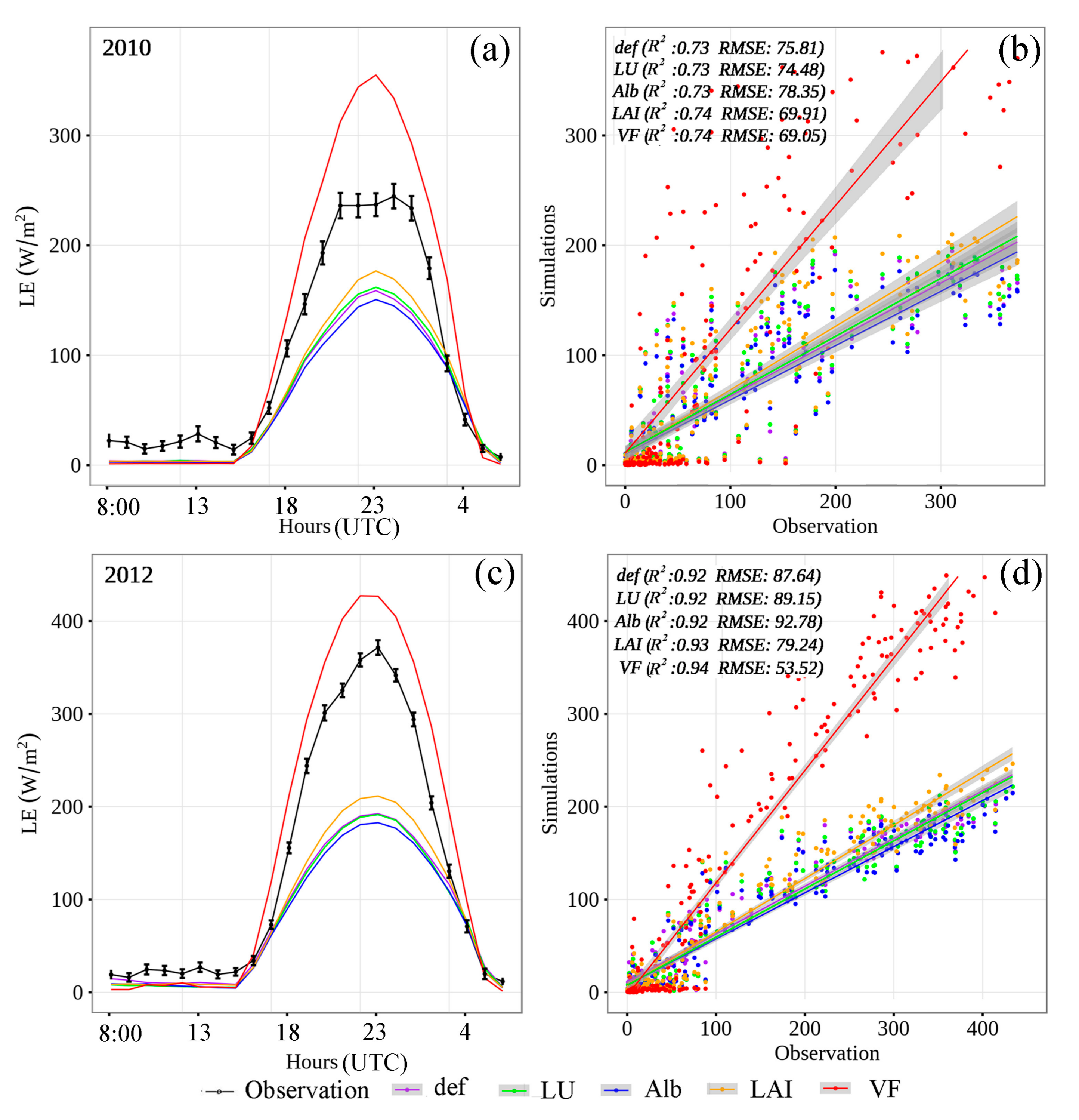
Figure 4.
Daytime spatial patterns of sensible heat flux (H) from the (a) def, (b) LU, (c) Alb, (d) LAI and (e) VF simulations, and their differences (f) b–a, (g) c–b, (h) d–c and (i) e–d (these difference pixels are statistically significant at p < 0.05). The def simulation used default LU, albedo, LAI, and VF provided by WRF itself; the LU simulation used only actual LU data; the Alb simulation used only actual LU and albedo data; the LAI simulation used actual LU, albedo, and LAI data, and the VF simulation used all of the actual terrestrial datasets. The red line represents the border of the key oasis area.
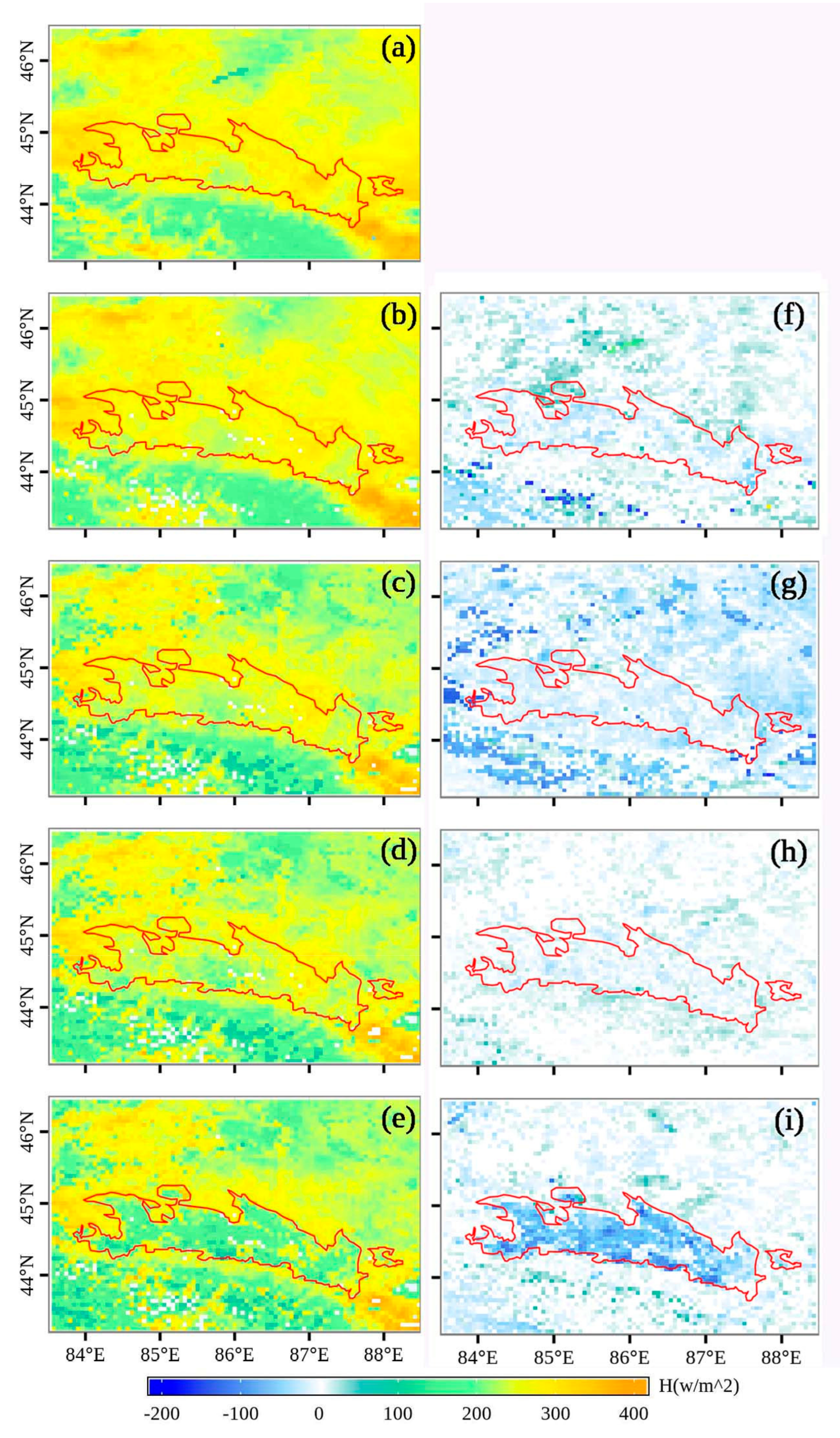
Figure 5.
Daytime spatial patterns of latent heat flux (LE) from the (a) def, (b) LU, (c) Alb, (d) LAI and (e) VF simulations, and their differences (f) b–a, (g) c–b, (h) d–c and (i) e–d (these difference pixels are statistically significant at p < 0.05). The def simulation used default LU, albedo, LAI, and VF provided by WRF itself; the LU simulation used only actual LU data; the Alb simulation used only actual LU and albedo data; the LAI simulation used actual LU, albedo, and LAI data, and the VF simulation used all of the actual terrestrial datasets. The red line represents the border of the key oasis area.
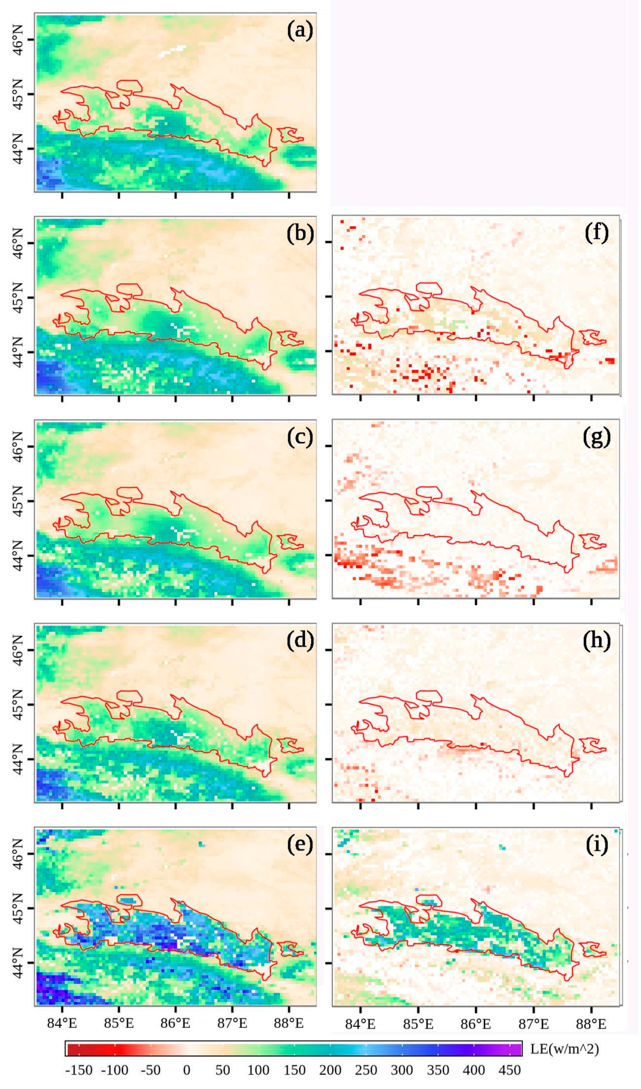
Figure 6.
Comparisons of hourly averaged 2 m air temperature (T2) between observations and five simulations (a,c,e,g,i,k), and corresponding scatter diagram (b,d,f,h,j,l) at six stations (S1–S6) in 2010 and 2012. The five simulations are as follows: def (using default LU, albedo, LAI, and VF data); LU (using actual LU data), Alb (using actual LU and albedo data), LAI (using actual LU, albedo, and LAI), and VF (using all of actual LU, albedo, LAI, and VF data).
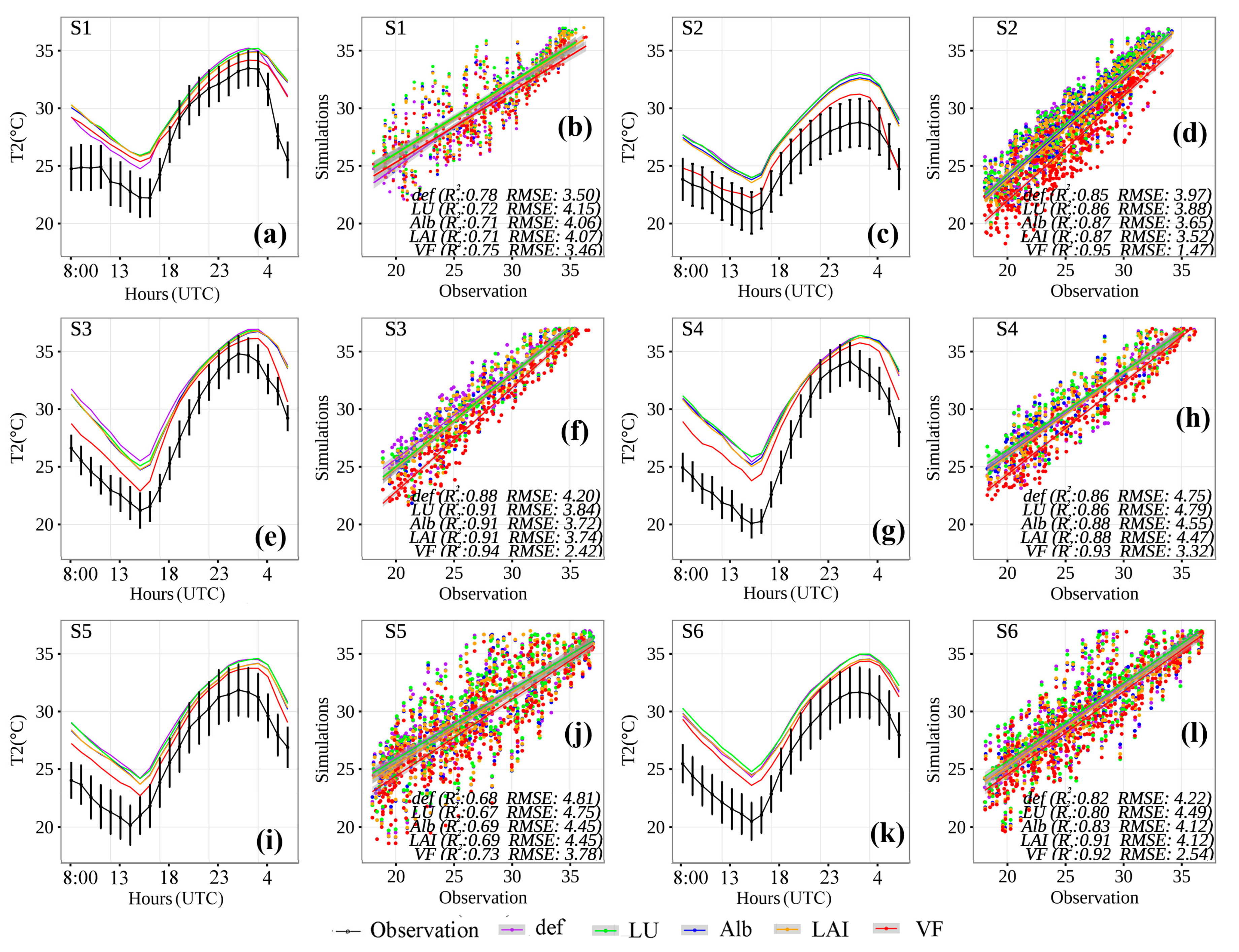
Figure 7.
Comparisons of hourly averaged 2 m relative humidity (RH) between observations and five simulations (a,c,e,g,i,k), and corresponding scatter diagram (b,d,f,h,j,l) at six stations (S1–S6) in 2010 and 2012. The five simulations are as follows: def (using default LU, albedo, LAI, and VF data); LU (using actual LU data), Alb (using actual LU and albedo data), LAI (using actual LU, albedo, and LAI), and VF (using all of actual LU, albedo, LAI, and VF data).
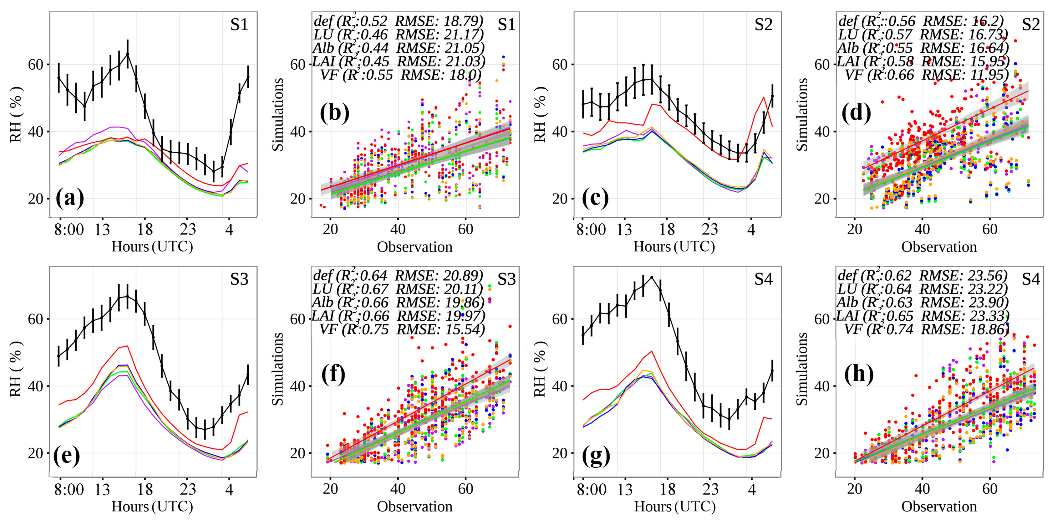
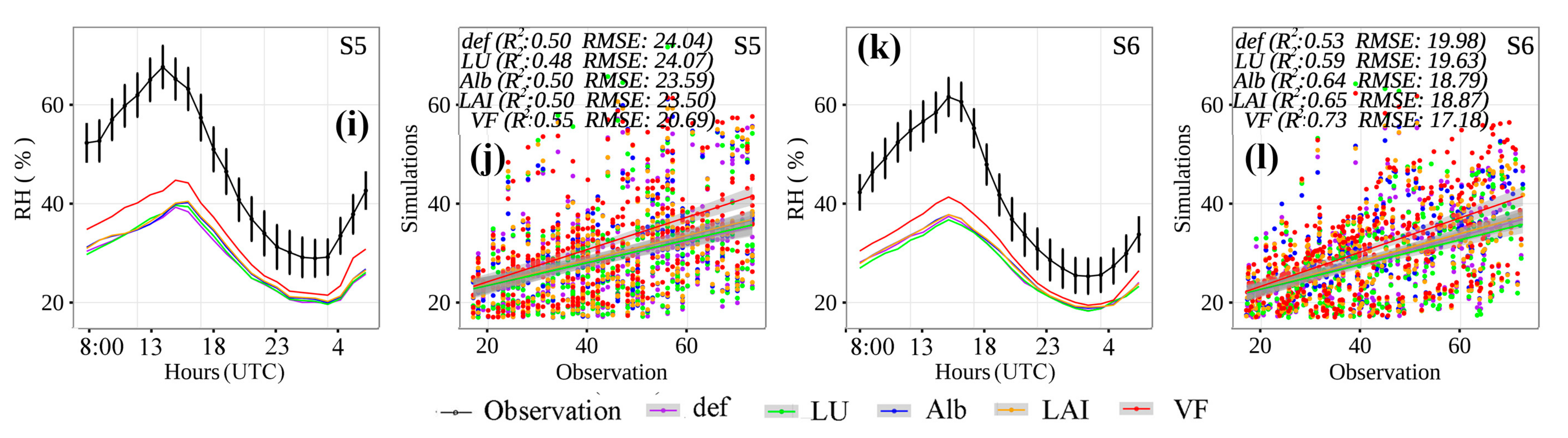
Figure 8.
Daytime spatial patterns of 2 m air temperature (T2) from the (a) def, (b) LU, (c) Alb, (d) LAI and (e) VF simulations, and their differences (f) b–a, (g) c–b, (h) d–c and (i) e–d (these difference pixels are statistically significant at p < 0.05). And corresponding patterns during the night-time, which are labelled with the corresponding daytime label and the number 1. The def simulation used default LU, albedo, LAI, and VF provided by WRF itself; the LU simulation used only actual LU data; the Alb simulation used only actual LU and albedo data; the LAI simulation used actual LU, albedo, and LAI data, and the VF simulation used all of the actual terrestrial datasets. The red line represents the border of the key oasis area.
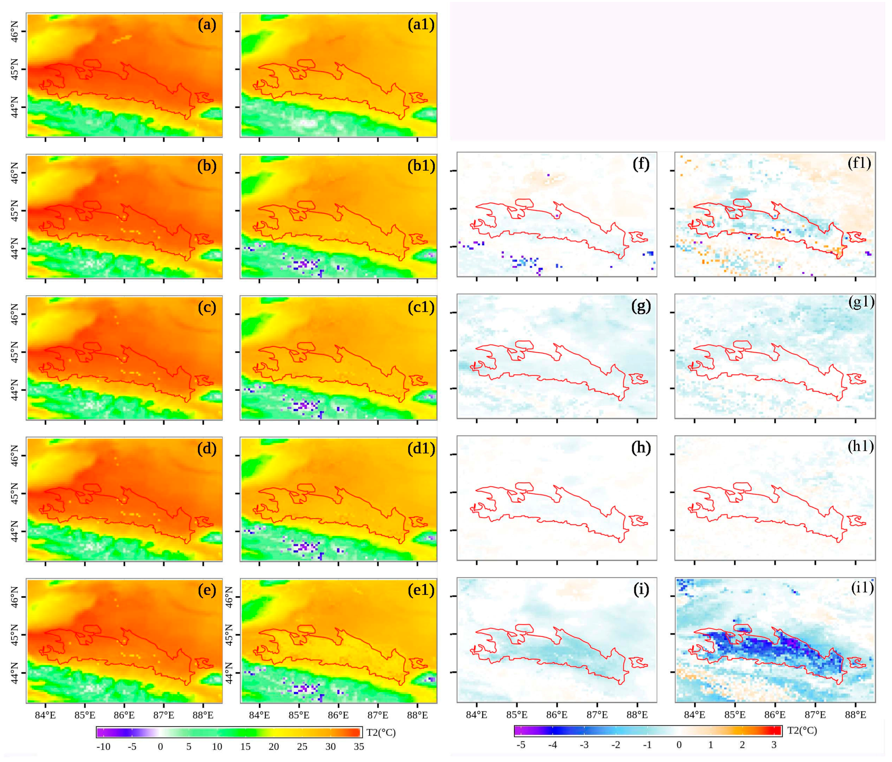
Figure 9.
Daytime spatial patterns of 2 m specific humidity patterns (Q2, g kg−1) from the (a) def, (b) LU, (c) Alb, (d) LAI and (e) VF simulations, and their differences (f) b–a, (g) c–b, (h) d–c and (i) e–d (these difference pixels are statistically significant at p < 0.05). And corresponding patterns during the night-time, which are labelled with the corresponding daytime label and the number 1. The def simulation used default LU, albedo, LAI, and VF provided by WRF itself; the LU simulation used only actual LU data; the Alb simulation used only actual LU and albedo data; the LAI simulation used actual LU, albedo, and LAI data, and the VF simulation used all of the actual terrestrial datasets. The red line represents the border of the key oasis area.

Figure 10.
Comparisons of hourly 10 m (a,c,e) wind speed (WS) and (b,d,f) wind direction (WD) between observations and five simulations at three stations (S1, S3, S4)
Figure 10.
Comparisons of hourly 10 m (a,c,e) wind speed (WS) and (b,d,f) wind direction (WD) between observations and five simulations at three stations (S1, S3, S4)
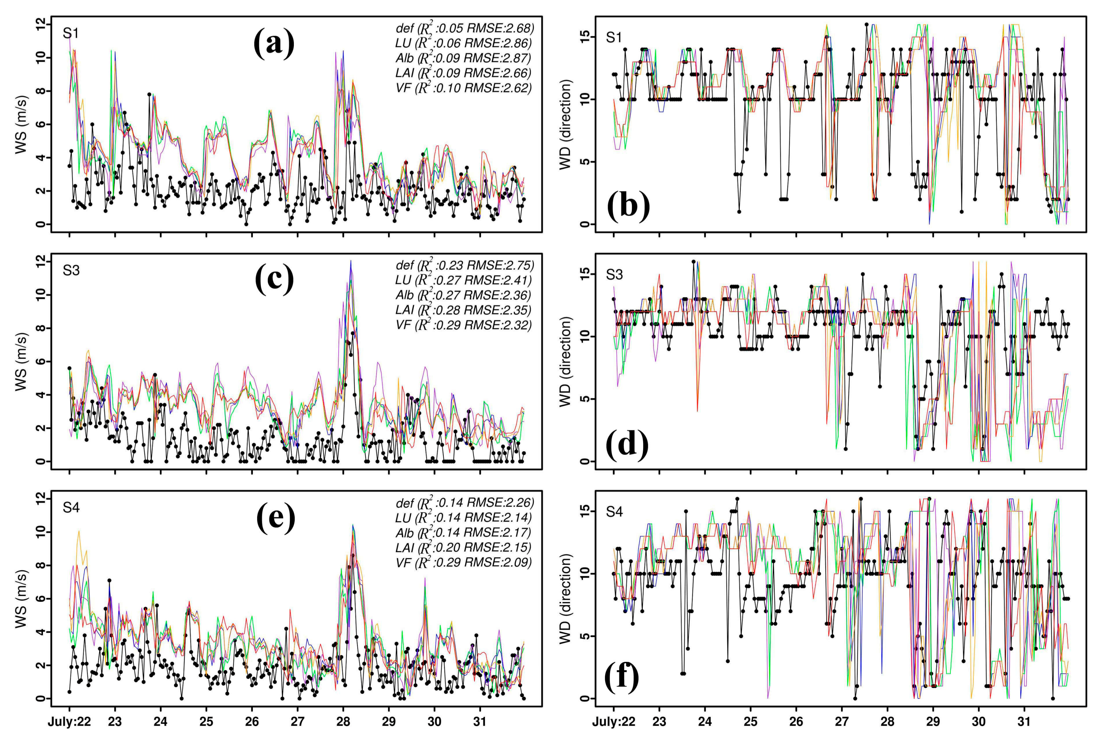
Figure 11.
Daytime spatial patterns of 10 m wind speed (WS) and wind direction (WD) from the (a) def, (b) LU, (c) Alb, (d) LAI and (e) VF simulations, and their differences (f) b–a, (g) c–b, (h) d–c and (i) e–d (these difference pixels are statistically significant at p < 0.05). And corresponding patterns during the night-time, which are labelled with the corresponding daytime label and the number 1. The def simulation used default LU, albedo, LAI, and VF provided by WRF itself; the LU simulation used only actual LU data; the Alb simulation used only actual LU and albedo data; the LAI simulation used actual LU, albedo, and LAI data, and the VF simulation used all of the actual terrestrial datasets. The red line represents the border of the key oasis area.
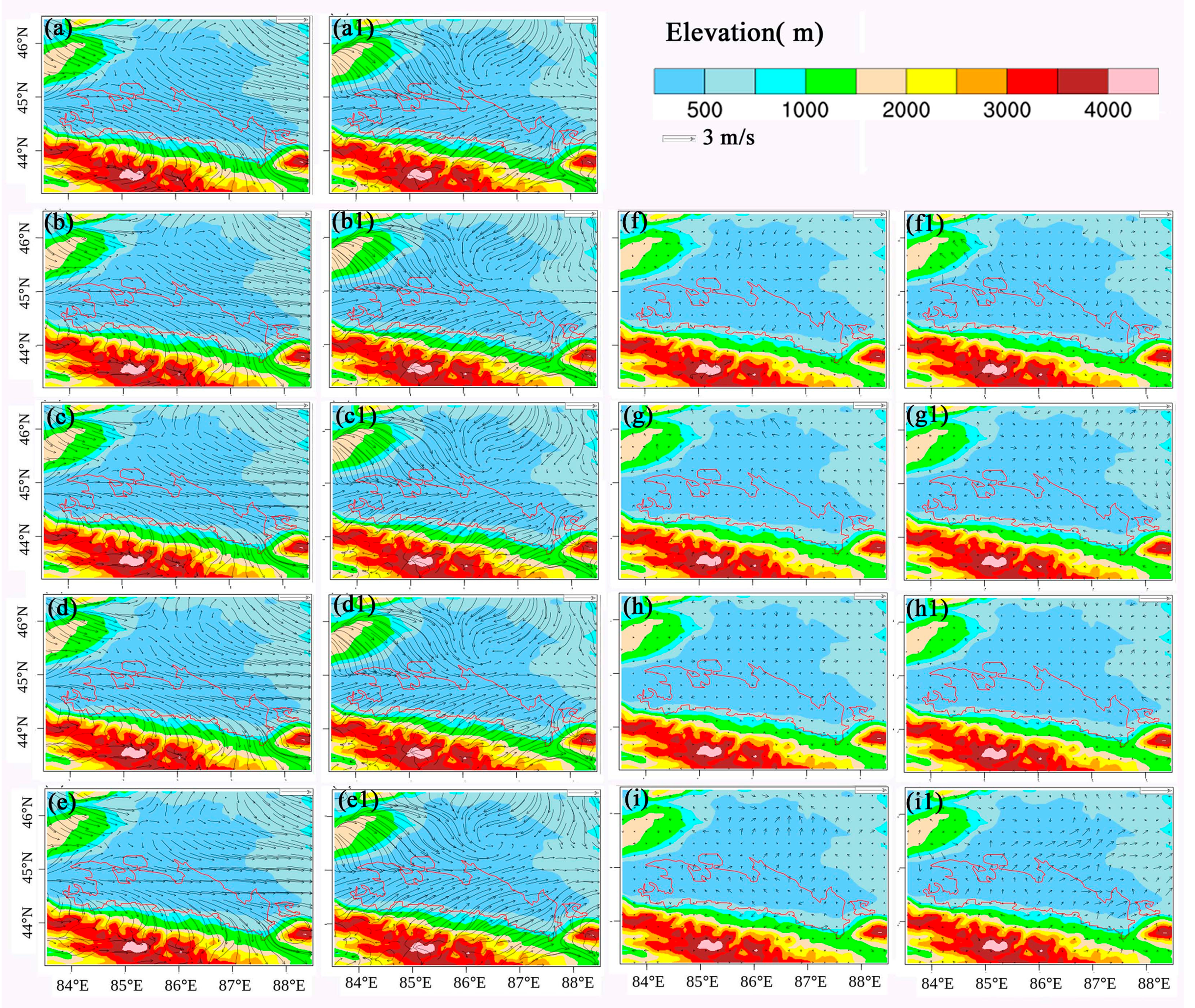
Figure 12.
Average bias percentages of simulated meteorological variables at six stations due to using each actual terrestrial dataset: (a) T2, (b) RH, (c) WS, (d) LE, (e) biases due to using actual LU data, (f) biases due to using actual albedo data, (g) biases using actual LAI data, and (h) biases due to using actual VF data.

Table 1.
Meteorological stations’ names, locations, elevations, and available elements.
| ID | Longitude/°E | Latitude/°N | Altitude/m | LU | Measurements | Time |
|---|---|---|---|---|---|---|
| S1 | 86.20 | 44.32 | 473.10 | Crop/Urban | T2, P, RH, WS, WD | 2012 |
| S2 | 85.82 | 44.28 | 469.30 | Crop | T2, RH, SW, LW, LE | 2010, 2012 |
| S3 | 85.25 | 44.85 | 338.10 | Crop | T2, P, RH, WS, WD | 2012 |
| S4 | 86.10 | 45.02 | 347.80 | Crop | T2, P, RH, WS, WD | 2012 |
| S5 | 87.93 | 44.29 | 476 | Desert | T2, RH | 2010, 2012 |
| S6 | 87.92 | 44.48 | 448 | Desert | T2, RH, | 2010, 2012 |
Note: LU represents land use; T2 represents 2 m air temperature; RH represents 2 m relative humidity; LE represents latent heat flux; WS and WD represent the wind speed and direction at 10 m, respectively; SW and LW represent the downward shortwave and longwave radiation, respectively.
Table 2.
Soil moisture values for the oasis and desert areas in the four Noah soil layers [42].
Table 2.
Soil moisture values for the oasis and desert areas in the four Noah soil layers [42].
| Land Use Type | Noah Soil Layer | Soil Moisture (cm3 cm−3) |
|---|---|---|
| Oasis | 0–10 cm | 0.38 (at 5 cm) |
| 10–40 cm | 0.47 (at 25 cm) | |
| 40–100 cm | 0.33 (at 70 cm) | |
| 100–200 cm | 0.26 (at 150 cm) | |
| Desert | 0–10 cm | 0.07 (at 5 cm) |
| 10–40 cm | 0.10 (at 25 cm) | |
| 40–100 cm | 0.05 (at 70 cm) | |
| 100–200 cm | 0.06 (at 150 cm) |
© 2017 by the authors. Licensee MDPI, Basel, Switzerland. This article is an open access article distributed under the terms and conditions of the Creative Commons Attribution (CC BY) license (http://creativecommons.org/licenses/by/4.0/).
Share and Cite
MDPI and ACS Style
Zhang, M.; Luo, G.; De Maeyer, P.; Cai, P.; Kurban, A. Improved Atmospheric Modelling of the Oasis-Desert System in Central Asia Using WRF with Actual Satellite Products. Remote Sens. 2017, 9, 1273. https://doi.org/10.3390/rs9121273
AMA Style
Zhang M, Luo G, De Maeyer P, Cai P, Kurban A. Improved Atmospheric Modelling of the Oasis-Desert System in Central Asia Using WRF with Actual Satellite Products. Remote Sensing. 2017; 9(12):1273. https://doi.org/10.3390/rs9121273
Chicago/Turabian StyleZhang, Miao, Geping Luo, Philippe De Maeyer, Peng Cai, and Alishir Kurban. 2017. "Improved Atmospheric Modelling of the Oasis-Desert System in Central Asia Using WRF with Actual Satellite Products" Remote Sensing 9, no. 12: 1273. https://doi.org/10.3390/rs9121273
Note that from the first issue of 2016, this journal uses article numbers instead of page numbers. See further details here.