Radiometric Correction of Simultaneously Acquired Landsat-7/Landsat-8 and Sentinel-2A Imagery Using Pseudoinvariant Areas (PIA): Contributing to the Landsat Time Series Legacy

Abstract

The use of Pseudoinvariant Areas (PIA) makes it possible to carry out a reasonably robust and automatic radiometric correction for long time series of remote sensing imagery, as shown in previous studies for large data sets of Landsat MSS, TM, and ETM+ imagery. In addition, they can be employed to obtain more coherence among remote sensing data from different sensors. The present work validates the use of PIA for the radiometric correction of pairs of images acquired almost simultaneously (Landsat-7 (ETM+) or Landsat-8 (OLI) and Sentinel-2A (MSI)). Four pairs of images from a region in SW Spain, corresponding to four different dates, together with field spectroradiometry measurements collected at the time of satellite overpass were used to evaluate a PIA-based radiometric correction. The results show a high coherence between sensors (r² = 0.964) and excellent correlations to in-situ data for the MiraMon implementation (r² > 0.9). Other methodological alternatives, ATCOR3 (ETM+, OLI, MSI), SAC-QGIS (ETM+, OLI, MSI), 6S-LEDAPS (ETM+), 6S-LaSRC (OLI), and Sen2Cor-SNAP (MSI), were also evaluated. Almost all of them, except for SAC-QGIS, provided similar results to the proposed PIA-based approach. Moreover, as the PIA-based approach can be applied to almost any image (even to images lacking of extra atmospheric information), it can also be used to solve the robust integration of data from new platforms, such as Landsat-8 or Sentinel-2, to enrich global data acquired since 1972 in the Landsat program. It thus contributes to the program’s continuity, a goal of great interest for the environmental, scientific, and technical community.

1. Introduction and Objective

Long time series of remotely sensed images are necessary for a large variety of applications that are related to Earth Observation (e.g., monitoring land cover change, studying surface temperature dynamics, etc.). One of the longest medium spatial resolution data sets is the Landsat Program. Images have been acquired in this program since 1972, and it is supervised by the National Aeronautics and Space Administration (NASA) and the United States Geological Survey (USGS). The Landsat Data Continuity Mission (LDCM) involves the use of different sensors (Multispectral Scanner System (MSS), Thematic Mapper (TM), Enhanced Thematic Mapper Plus (ETM+), and Operational Land Imager (OLI)), having in common to be sensitive in the region of the electromagnetic spectrum comprised between visible and short wave infrared regions (about 400 nm and 2350 nm) [1]. The LDCM also includes the Return Beam Vidicon (RBV) camera, thermal bands (in the MSS of Landsat-3 and TM/ETM+), and thermal sensors (Thermal Infrared Sensor, TIRS in Landsat-8), which are out of the focus of this paper. Currently, images are still acquired from ETM+, on board Landsat-7, and from OLI, on board Landsat-8. Recently, new sensors with similar spectral characteristics are complementing the Landsat program within the Global Earth Observation System of Systems (GEOSS) [2]. Among them, the Multispectral Imager (MSI) sensor on board the two Sentinel-2 satellites (European Space Agency, ESA) is especially relevant, providing imagery since 2015 (Sentinel-2A) and 2017 (Sentinel-2B) [3], with improved characteristics that are specifically designed to support the Landsat Program [4,5]. Several efforts have been made to review the Landsat Legacy inter-sensor comparison, or to even compare them to other sensors, such as ALI (EO-1) [6,7]. For instance, Mishra et al. [8] used Pseudo Invariant Calibration Sites (PICS), which are spatially uniform sites spectrally stable over time, for on-orbit calibration of Landsat-5 through Landsat-8, and Czapla-Myers et al. [9] used Radiometric Calibration Test Sites that are permanently monitored for Landsat-8. In 2016, ESA completed the processing of its MSS, TM, ETM+, and OLI Level 1 historical archive, and used PICS to validate the inter-sensor coherence between OLI and MSI [10]. Gascon et al. [11] describes Sentinel-2A performance in depth and validates it using PICS and in-situ surface reflectance data. In-situ radiometric measurements, together with sensors with higher spectral but coarser spatial resolution, such as MODIS, are also widely used to validate Landsat and Landsat-like sensors by the Committee on Earth Observation Satellites—Working Group on Calibration and Validation (CEOS-WGCV) [12]—and others [13,14]. Recently, NASA [15] presented a Harmonized Landsat-8 and Sentinel-2 (HLS) product. This is a very interesting product that adopts the tiling system of Sentinel-2 data (Military Grid Reference System, MGRS) and resamples MSI data (10 m or 20 m) to the spatial resolution of OLI (30 m). However, this product does not fit the purpose of this paper due to the unavailability of HLS imagery in some areas that are used in our study and the absence of ETM+ images, as well as the pixel upscaling of MSI imagery. Since 2016, an international collaborative initiative called CEOS-WGCV Atmospheric Correction Inter-comparison Exercise (ACIX) [16] has focused on the results of several atmospheric correction processors that are applied to OLI and MSI imagery from global test sites. Methods are compared by validating the aerosol optical depth and the water vapor content output products with the Aerosol Robotic Network (AERONET) [17] measurements and by validating the surface reflectance results from different approaches with their output time series (one year) with the MODIS (MOD09GA) daily surface reflectance 500 m product, and with fiducial reference measurements [16].

In order to be fully comparable, imagery that were acquired on different dates and by different sensors has to be converted to surface reflectance products through radiometric corrections (atmospheric, and, ideally, also including topographic corrections) [18,19,20,21,22,23,24]. With these corrections, at-sensor spectral radiance (Ls_λ) (W·m⁻²·sr⁻²·µm⁻¹) is converted to surface spectral reflectance (ρs_λ) (dimensionless), removing atmospheric effects and accounting for the illumination effects derived from the Sun position (θs, ϕs), the terrain morphology, and the sensor position (θv, ϕv), where θ is the zenith angle and ϕ is the azimuth angle. Most atmospheric gases and aerosols cause effects like scattering, absorption, and polarization of solar radiation, which lead to changes in the incoming irradiance [19,20]. Indeed, through its path from the Top of Atmosphere (TOA) to the Bottom of Atmosphere (BOA) (downwelling path), and back to the sensor once reflected (upwelling path), the energy is scattered and absorbed causing the extinction of the initial energy flux (exoatmospheric spectral irradiance (E_SUNλ) (W·m⁻²·µm⁻¹)). This phenomenon of light extinction is quantified with the spectral magnitude known as atmospheric transmittance (τ_λ) (dimensionless). Transmittance is dependent on spectral atmospheric Total Optical Depth (TOD) (τ_0λ), as greater TOD implies lower transmittances. Transmittance is also dependent on the zenith angle of the illumination vector (the greater the angle the smaller the transmittance). Simultaneously, scattering leads to energy redistribution, and, a part of this energy flux contributes, as diffuse radiance (atmospheric spectral radiance, Latm_λ (W·m⁻²·sr⁻²·µm⁻¹)), to the radiance received both at the Earth’s surface and at the sensor. Therefore, in general terms, atmospheric corrections of the signal reflected from the Earth’s surface have two main unknowns (wavelength dependent) [25]: the Total Optical Depth that weakens the signal, and the atmospheric radiance that contributes to the signal in addition to the reflected beam.

According to this theoretical context, many approaches have been developed to obtain atmospherically corrected surface reflectance data from multispectral imagery in the solar spectrum. These approaches can be summarized into three main groups: the physically based approaches, the image based approaches, and the radiometric reference approaches.

Physical approaches: The most tuned technique is the use of a Radiative Transfer Model (RTM), which accurately calculates the physical effects of the atmosphere over the entire light path, and for which several approaches exist (SCIATRAN [26,27], 6SV1 [28,29], DISORT [30,31], ARTS [32], 4A/OP [33], MODTRAN [34], or libRadtran [35]). Sophisticated physical RTM account for polarization effects, which involve complex calculations due to the dependency of the resulting phase function on the shape of the particle that interacts with the energy (further information on the inclusion of polarization in RTM can be found in the work of Kokhanovsky [19,36,37,38]). All of these physical RTM are usually very time consuming and need to be fed with accurate atmospheric composition data (e.g., water vapor content, ozone content, aerosol size, and distribution, etc.), which are sometimes obtained from other satellite sensors (MODIS [13] or SCIAMACHY [39]) or from auxiliary information, but ideally from in-situ atmospheric measurements. Although it is currently possible to obtain local atmospheric information from all over the world through global initiatives, such as AERONET (1379 sites on July 2017, some of them currently unavailable [40]), the spatial and temporal coverage of these measurements are scarce when going backwards, especially before 2000 (in 1997 nearly 60 locations contributed to the database) [17].

Image based approaches: Although physical approaches usually obtain better agreement, the unavailability of the data needed to run these models, especially data close in time and/or space to the target image, has led to the wide use of other techniques that avoid using remote or in-situ atmospheric measurements. These approaches are based on the Dark Object Subtraction method (DOS) [23] that assumes the existence of image pixels that should provide a close to zero radiance (dark objects), and assigns, at each band, their value to the atmospheric signal. The at-sensor digital numbers (DN) are converted to spectral radiances using calibration coefficients (gain and bias) that are provided in the image metadata or in specific calibration review works, to later subtract the atmospheric radiance value from every pixel in the atmospheric correction. Several versions of the DOS method make different assumptions about the threshold of the atmospheric radiance determination (histogram properties, minimum value, dense dark vegetation (DDV), etc.). The most basic version assumes total transmittance (τ = 1), and does not account for the diffuse radiance contribution to the target irradiance. The COST version [41] models the downwelling transmittance as a function of the cosine of the Sun zenith angle (θs). Further approaches incorporate upwelling transmittance as a function of the cosine of the view zenith angle (θv), and account for the diffuse radiance that is affecting the target [13].

Radiometric reference approaches: These approaches use radiometric reference values (either from invariant objects or from field data measurements taken simultaneously at satellite pass) to obtain the unknowns of the physical model (mainly atmospheric ones). In the case of the invariant object method, it is assumed that an image contains target areas with well-known and stable reflectance; the correction is carried out to fit the reflectance of these target areas to their radiometric reference values. A general approach to the invariant object technique was proposed by Hall et al. [42], who intended to obtain a common radiometric response for corrected images that were acquired by different sensors on different dates through “radiometric control sets”, which are nonvegetated extremes of the Kauth–Thomas brightness-greenness scattergram; note that these authors point out that “the members of the radiometric control sets may not be the same pixels from image to image”. Hadjimitsis et al. [21] used pseudoinvariant targets to atmospherically correct time series with high quality results. Pons et al. [43] presented a hybrid technique between DOS and pseudoinvariant areas (PIA), fitting spectral TOD (τ_0λ), and spectral atmospheric radiance (Latm_λ) unknowns to match reference values of radiometrically stable areas, which were extracted from existing 10-year surface reflectance TERRA-MODIS products (MOD09GA). The method was able to automatically generate surface reflectance products from MSS, TM, and ETM+ imagery, being validated throughout spectral signature comparisons with Landsat and MODIS official surface reflectance products to evaluate the signature coherence in several land covers (built-up areas, Aleppo pine forests, Scots pine forests, holm oak forests), while the time-series robustness was evaluated with testing PIA not used the radiometric correction procedure (σ_blue = 0.54%; σ_green = 0.68%; σ_red = 0.69%; σ_NIR = 1.81%; σ_SWIR1 = 1.56%; and, σ_SWIR2 = 0.96%). PIA-based method also yielded good results for land cover classification of multisensory data from the Iberian Peninsula (1980–2015) [44]. In the case of radiometric field data acquired simultaneously to the capture of the image, the measurements are used in a similar way as in the previous case, but these measurements can only be used as a reference to correct the image acquired simultaneously.

In all three approaches, some sophistications make use of Digital Elevation Models (DEM) to consider the terrain effects on the illumination angle, and therefore, improve the accuracy by accounting for the amount of energy the surface receives per unit surface [18].

Alternatively to these three approaches, it is also possible to simply use a purely empirical line fitting. The empirical line fitting approach needs in-situ spectroradiometric measurements at satellite overpass to correct the whole radiance image by adjusting each band to at-surface reflectance measured values through linear regression [45,46], instead of using the data to obtain the unknowns of a physical model. However, this technique is not operational for backdated images or when a complete spatio-temporal field spectroradiometric measurements campaign is needed for a large area, and for that reason, some authors proposed linear fittings using pseudoinvariant features (PIF) [47].

The objective of this paper is to validate the performance of the PIA-based radiometric correction for the current ETM+, OLI, and MSI imagery (since for MSS-TM-ETM+ has already been validated in Pons et al. [43]).

The hypothesis of the present study is that surface reflectance retrieved from ETM+, OLI, and MSI imagery by the PIA-based approach is at least as good as that of other analyzed methods when compared to field data, and, because it has the advantage of allowing backdate radiometric image correction, this approach can contribute to complementing the Landsat time series legacy by adding Landsat-like sensors.

An experiment was designed to compare surface reflectances obtained through a PIA methodology (on ETM+, OLI, and MSI, MiraMon implementation) with field spectroradiometric data acquired at satellite overpass. Moreover, this field data was also compared with the results of commonly used atmospheric correction algorithms, such as ATmospheric CORrection (ATCOR3) [48] on ETM+, OLI, and MSI imagery, Semi-Automatic Classification plug-in implemented in QGIS (SAC-QGIS) [49] on ETM+, OLI, and MSI imagery, Second Simulation of a Satellite Signal in the Solar Spectrum—Landsat Ecosystem Disturbance Adaptive Processing System (6S-LEDAPS) [50] on ETM+ imagery, Landsat Surface Reflectance Code (6S-LaSRC) [51] on OLI imagery, and Sen2Cor implemented in SeNtinel’s Application Platform (Sen2Cor-SNAP) [52] on MSI imagery. Finally, the inter-sensor coherence of each radiometric correction method was evaluated by comparing the results of Landsat and Sentinel simultaneous acquisitions in the sampled pixels.

2. Study Area, Materials and Methods

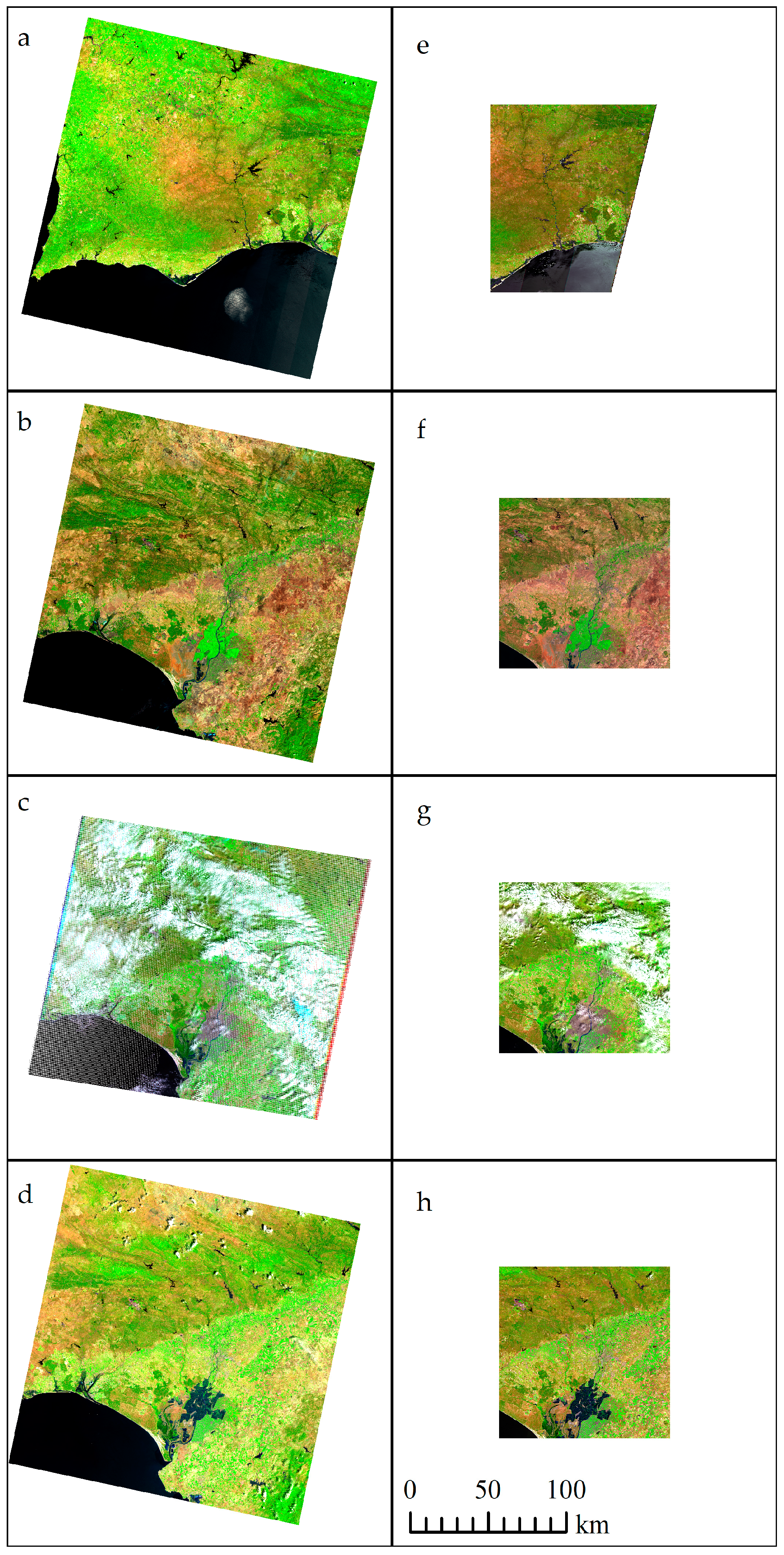
2.1. Study Area

The study area is located in the region of the Doñana National Park (DNP), SW Spain, and also in SW Europe (Figure 1). Field spectroradiometry and model evaluation was performed in two different sub-areas, “Villanueva de los Castillejos” in the surroundings of the DNP under the scenes R037-29SPB (Sentinel-2 MGRS orbit and tile system [53]) and 203-034 (Landsat World Reference System-2 (WRS-2) path and row system [54]), and “Laguna de Santa Olalla” sub-area inside the DNP under the scenes R137-29SQB and 202-034. Besides the great ecological interest of the study area, it is a flat region and is at sea level. These characteristics mean that methods that do not account for relief illumination effects (such as SAC-QGIS, 6S-LEDAPS, or 6S-LaSRC) can be fairly compared to those that do account for relief illumination effects (such as ATCOR3, Sen2Cor-SNAP, or PIA-MiraMon). However, a method that includes a rigorous topographic correction would need to be considered in other regions with a rugged terrain.

2.2. Materials

2.2.1. Satellite Data: Landsat-7 ETM+, Landsat-8 OLI and Sentinel-2A MSI

Landsat-7 and Landsat-8 L1T (Level 1 T: precision terrain-corrected to UTM 29N, WGS84, TOA radiances products) images and the L2A (Level 2 A: geometry as L1T and surface reflectances corrected for atmospheric effects with a cloud mask, a cloud shadow mask, and a water and snow mask) official products were obtained from the USGS website through the EarthExplorer tool [55] (Figure 2). Sentinel-2A L1C (Level 1 C: product results from using a Digital Elevation Model to project the image in cartographic geometry (UTM 29N, WGS84); per-pixel radiometric measurements are provided in TOA reflectances) images and the L2A (Level 2 A: BOA reflectances in cartographic geometry (as L1C)) official products were obtained from the website of the European Space Agency (ESA)—Copernicus through the Scientific Data Hub tool [56] (Figure 2). The time and date of imagery acquisition are shown in

Table 1. Features of Landsat-7, Landsat-8 and Sentinel-2A imagery used in the study.

Path/Orbit	Row/Granule	Date of Acquisition	Sun Elevation (Plot Area)	Sun Azimuth (Plot Area)	View Zenith Angle (Plot Area)	Start Time (UTC)	Source	Sensor
203	034	20 May 2016	65.72°	130.47°	3.16°	11:08:03	USGS	OLI
R037	T29SPB		68.70°	140.77°	8.72°	11:29:04	ESA	MSI
202	034	4 October 2016	45.12°	153.91°	0.90°	11:02:33	USGS	OLI
R137	T29SQB		45.72°	156.32°	2.73°	11:09:12	ESA	MSI
202	034	22 April 2017	59.59°	139.03°	0.61°	11:04:57	USGS	ETM+
R137	T29SQB		59.90°	140.01°	2.49°	11:06:51	ESA	MSI
202	034	1 June 2017	66.60°	124.39°	0.89°	11:02:09	USGS	OLI
R137	T29SQB		67.77°	126.71°	2.50°	11:06:51	ESA	MSI

.

The Sentinel-2 and Landsat sensors studied in this paper have six bands that correspond to each other. The spectral configuration of the ETM+ [57], OLI [58], and MSI [59] sensors has common matching bands in the blue, green, red, and short wave infrared (SWIR) regions (

Table 2. Band correspondence between Multispectral Scanner System (MSS) (example for Landsat-1), Thematic Mapper (TM) (example for Landsat-5), Enhanced Thematic Mapper Plus (ETM+), Landsat-8 (OLI) and Sentinel-2A (MSI) (example for Sentinel-2A), fitting the continuity of the Landsat Program.

	Bandwidths (nm) (#: Band Number)
Sensor	Blue	Green	Red	NIR	SWIR1	SWIR2
MSS 1		504–602 (#4)	605–701 (#5)	811–990 (#7)
TM 2	452–518 (#1)	528–626 (#2)	626–710 (#3)	776–904 (#4)	1567–1785 (#5)	2096–2350 (#7)
ETM+ 3	441–514 (#1)	519–611 (#2)	631–692 (#3)	772–898 (#4)	1547–1748 (#5)	2064–2346 (#7)
OLI 4	452–512 (#2)	533–590 (#3)	636–673 (#4)	851–879 (#5)	1567–1651 (#6)	2107–2294 (#7)
MSI 5	470–524 (#2)	543–578 (#3)	649–680 (#4)	782–898 (#8) 855–875 (#8a)	1569–1658 (#11)	2113–2286 (#12)

¹ Full Width Half Maximum (FWHM) of MSS in Landsat-1 [62]; ² FWHM of TM in Landsat-5 [63]; ³ FWHM of ETM+ [57]; ⁴ FWHM of OLI [58]; ⁵ FWHM of MSI in Sentinel-2A [59].

). Nevertheless, in the near infrared (NIR) region, the ETM+ NIR band is wider than the OLI NIR band, corresponding to MSI band 8 and band 8a, respectively. OLI bands are located in the same spectral regions as previous Landsat sensors to ensure spectral continuity [60], and MSI bands are located in the same regions to fit the heritage of Landsat and SPOT Copernicus Service Elements [61]. In other words, the bands that have the longest continuity in the LDCM are those that are located in the visible (VIS) and NIR since the Multispectral Scanner System (MSS) sensor [62], while since the Thematic Mapper (TM) [62], there is continuity in the two SWIR bands, as shown in Table 2. Besides, the Sentinel-2A MSI instrument has three channels in the red edge region (697.5 nm–793 nm) [59] that do not match the ETM+ or OLI sensors, and, for this reason, they are out of the scope of this work.

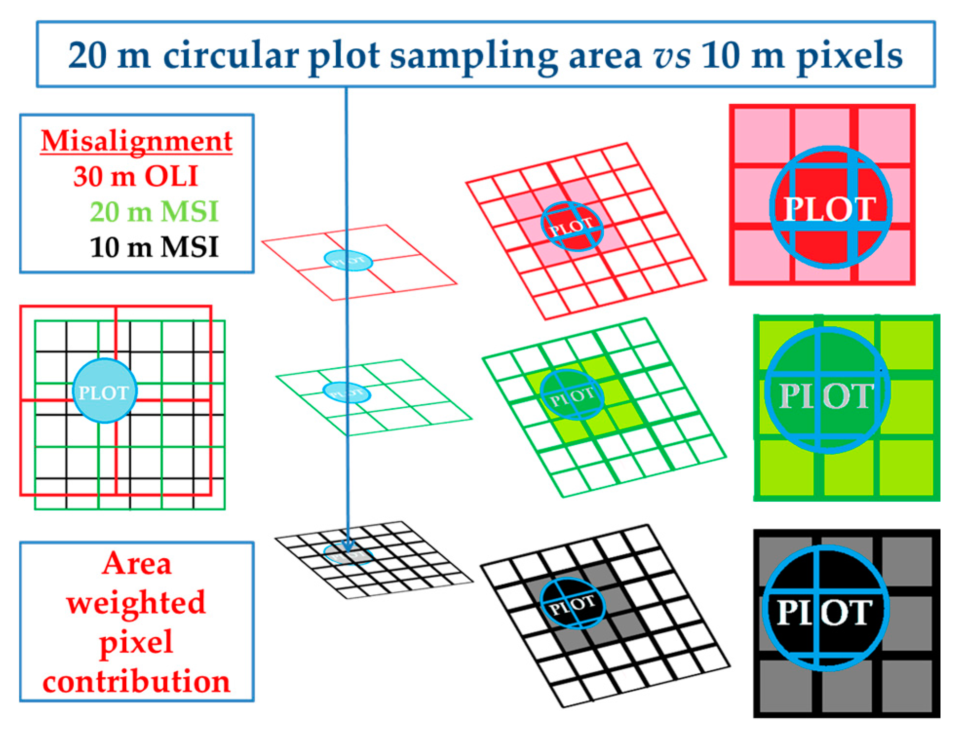
2.2.2. Field Data: Instrument, Protocol and Sample Data

Field spectroradiometric measurements were acquired by the Remote Sensing and GIS Laboratory Doñana Biological station, Spanish Council for Scientific Research (LAST-EBD (CSIC)), following the Jiménez and Díaz-Delgado [64] methodology, which has been widely used in previous airborne and field campaigns [65,66]. The spectroradiometer used was an ASD FieldSpec3 (Analytical Spectral Devices, Boulder, CO, USA). The spectral range covers the VIS, NIR, and SWIR regions (350 nm–2500 nm), with a spectral resolution (Full Width Half Maximum, FWHM) of 3 nm for the VNIR region (350 nm–1000 nm) and 10 nm for the SWIR region (1000 nm–2500 nm), even though the sampling intervals are 1.4 nm and 2 nm, respectively [67]. Field spectroradiometry sampling areas were designed with a circular shape with a diameter of 20 m. Measurements were taken facing the Sun (to avoid self-shadows) and were collected by sweeping the circle in a zigzag pattern advancing towards the Sun; in the case of water, we made punctual measurements, while remaining as fixed as possible in the selected water area, following the protocols stated in Peña-Martinez et al. [68] and Mueller et al. [69]. The pointer was located in zenithal position at 150 cm above the ground (nadir view), resulting in a footprint of 65–70 cm (Figure 3a). 20 to 40 measurements were made at each sampling plot and its arithmetic mean, median, and standard deviation was calculated. The reflectance of each land cover was obtained by dividing the average target radiance by the average (10 scans) of a white (Spectralon) reference panel radiance [70]. The two measurements were acquired alternatively and the instrument dark current was measured before each sampling [71,72]. Together with the radiometric measurements, its metadata was taken on the field with a Trimble PDA NOMAD with GPS and Cybertracker software, storing the time, date, location, etc. The accuracy of the GPS is about 5 m, but the areas where the sampling points were made are large and homogeneous enough to be sure that there was no problem correlating with the appropriate pixels. In the present work, the sampling area was previously identified as a homogeneous and flat land cover, including shallow lake water with presence of filamentous algae (Cladophora fracta) (Figure 3b), sand of dune (Figure 3c), senescent wheat crops, albero (organic ochre sandy clay (Figure 3d)), loamy sand of the dry shallow lake littoral zone, open grasslands (mainly Vulpia membranacea and Malcolmia triloba), shrubs (Halimium halimifolium and Lavandula stoechas (Figure 3f)), grasslands (mainly Poa bulbosa and Trifolium subterraneum (Figure 3e)), or active fern vegetation. Regarding the sampling points within the National Park near Laguna Santa Olalla, they have been used previously by our team in studies with airborne hyperspectral sensors since 2008. It is a well-known area of easy access and with a diverse land cover, of an adequate size, and where the different covers are very close to each other, being able to go from a lake of permanent waters to a dune with very reflective sand in a few minutes (a key characteristic for radiometric studies), and all of this in a protected area with different kinds of natural vegetation. Regarding those located in Villanueva de los Castillejos, they were selected in order to also test over a different satellite orbit and covers (water bodies used for irrigation and to water cattle, large extensions of homogeneous grasslands, etc.). On the outskirts of the town, there is a soccer field covered of albero that was also considered potentially interesting, as well as diverse crop fields of easy access.

2.2.3. Field Data: Campaigns

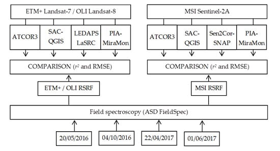
On 20 May 2016, concurrently at Landsat-8 and Sentinel-2A overpass, five spectral measurements were collected at five locations in Villanueva de los Castillejos, Huelva (Spain). This zone is close to, but not inside the DNP. The interest of this experimental zone resided in the presence of senescent wheat crops, albero (x2) and meadow (x2) samples (Figure 4a,b). The meteorological conditions were good, but not optimum due to some cirrus coming from the south of the scene (Figure 2a,e). A measurement was made in water but it has been discarded of the study due to a sunglint in the Sentinel-2A image (Figure 4b).

On 4 October 2016, concurrently at Landsat-8 and Sentinel-2A overpass, six spectral measurements were collected at six locations near Laguna de Santa Olalla, previously used for remote sensing airborne campaigns [65,66], inside the DNP. This zone allows for the rapid acquisition of spectral measurements of shallow lake water, sand-dune (x2), dry shallow lake littoral zone (loamy sand) (x2), and bracken (active fern vegetation) (Figure 4c). The meteorological conditions were good (Figure 2b,f).

On 22 April 2017, concurrently at Landsat-7 and Sentinel-2A overpass, six spectral measurements were collected at six locations in the same area around Laguna de Santa Olalla as the area that was sampled in October 2016. In this campaign, samples of shallow lake water (x2), sand-dunes (x2), open grassland, and shrub vegetation were taken (Figure 4c). The meteorological conditions were good over this site, but the full satellite scene includes heavy clouded areas that are surrounding DNP (54% cloud cover in the ETM+ image and 11% in the MSI image) (Figure 2c,g). Note that this area is located at the central strip of the ETM+ scene, and therefore was not affected by the Scan-Line Corrector failure (SLC-off) gaps (SLC compensates for the forward motion of the satellite, and failed on 2003, causing images having wedge-shaped gaps that range from a single pixel in width near the image-nadir, to about 12 pixels towards the edges of the scene; geostatistical methods [73] and neighbor interpolation methods [74] are commonly used to fill these gaps when needed).

On 1 June 2017, concurrently at Landsat-8 and Sentinel-2A overpass, nine spectral measurements were collected at nine locations in the same area of Laguna de Santa Olalla. In this campaign, samples of shallow lake water (x3), sand-dunes (x2), shrubs (x2), open grassland, and bracken were acquired (Figure 4c). The meteorological conditions were excellent (Figure 2d and Figure 3h).

2.3. Methods

2.3.1. Method 1: ATCOR Based Radiometric Corrections (ATCOR3 and Sen2Cor-SNAP)

In this study, we used the ATCOR3 software for ETM+/OLI/MSI corrections, while the Sen2Cor-SNAP software was used for MSI corrections. The code used in ATCOR3 [48] is also embedded in Sen2Cor-SNAP [75], performing atmospheric and topographic corrections [48]. The atmospheric radiance is obtained through DDV pixels, identified in an initial TOA pre-classification [48] (p. 220). DDV pixels are used as a reference assuming a known reflectance and adjusting the model to the TOD and atmospheric radiance stored in a Look-Up Table (LUT), pre-calculated with MODerate resolution atmospheric TRANsmission (MODTRAN 5). This fitting serves to define the MODTRAN 5 aerosol model that best fits the image. Once the aerosol type is chosen, transmittance is provided by a LUT, accounting for solar position, path length, and the physical components of TOD (τ₀): Rayleigh scattering, molecular absorption (O₃, H₂O, CO₂), and aerosol scattering. Sen2Cor-SNAP provides additional features described by Pflug [76]. As noted in the Sen2Cor Algorithm Theoretical Basis Document (ATBD), LUTs for ATCOR3 are based on MODTRAN 5, while Sen2Cor LUTs are based on the Library for Radiative Transfer (libRadtran) [75] (p. 6). Another difference between Sen2Cor and ATCOR3 is the use of the European Center for Medium-Range Weather Forecast (ECMWF) aerosol database when DDV are missing within the scene [76]. If a DEM is used for topographic correction, then the illumination effects are corrected (from local zenith angle, slope, and aspect), and the percentage of the sky viewed for every pixel and their adjacency effects are taken into account [75]. We used “Aerosol Type = Rural” and “Water Vapor Category = Mid-latitude summer (water vapor column: 2.92 cm for sea level)” for Landsat ATCOR3 atmospheric corrections of all of the months except for 4 October 2016 images, where was used Water “Vapor Category = Fall/Spring (water vapor column: 1.14 cm for sea level)”. For Sentinel-2A imagery ATCOR-based algorithms presented best results with “Aerosol Type = Rural” and automatically detecting WV LUT category using band #9 and in Sen2Cor specific case using the standard Atmospheric Precorrected Differential Absorption (APDA) model. The same DEM was used in ATCOR3 and PIA-MiraMon Landsat and Sentinel imagery for topographic corrections and for the estimation of atmospheric parameters as function of height, a very detailed 5 m DEM from Plan Nacional de Ortofotografía Aérea (PNOA) [77], resampled and aligned by bilinear interpolation at 10 m, 20 m and 30 m to fit the different spatial resolutions involved. The Sen2Cor official products used the Shuttle Radar Topographic Mission (SRTM) 90 m DEM [78] default option for the same previous purposes.

2.3.2. Method 2: Semi-Automatic Classification (SAC-QGIS)

Semi-Automatic Classification (SAC) is a plug-in implemented in QGIS, which is designed to perform a land cover classification quickly, but an atmospheric correction is carried out in the pre-processing step [49]. This atmospheric correction is based on the basic DOS technique, inspired by Chavez [41] and Moran et al. [79], which approximates the path radiance value of a given band from the minimum value of the histogram (dark object), assuming an intrinsic reflectance of this object. This approximation assumes that the darkest object of the scene must have a reflectance (1%), but the rest of the radiance that is received by the satellite sensor proceeds from the atmospheric path, and must be then subtracted from every pixel before dividing the at-sensor spectral radiance by the irradiance. The model assumes that the transmittance is 1 [49], considering total atmospheric transparency in all of the images, which simplifies the model, but at the same time could act as a source of error. The SAC-QGIS method is quick and simple, fully image-based, avoiding the need for atmospheric auxiliary data to perform the correction. Nevertheless, it does not approximate the TOD and does not account for topographic effects, a characteristic that is not relevant in the present study due to the flat morphology of the study area, but it is highly relevant in mountainous areas [80], although there are studies suggesting that topographic correction may not be justified in change detection routines computing spectral trends from pixel-based composites [81].

2.3.3. Method 3: 6S Based Radiometric Corrections (Landsat Surface Reflectance Code (LaSRC) and Landsat Ecosystem Disturbance Adaptive Processing System (LEDAPS) Atmospheric Correction)

The Landsat Surface Reflectance Code (LaSRC) [24,51] is a code that is designed to obtain Level 2A products, that is, to transform TOA radiance to surface reflectance. This code is based on the Second Simulation of the Satellite Signal in the Solar Spectrum (6S) [28,29] radiative transfer code. 6S uses a sophisticated procedure [82] that has been successfully validated and implemented for previous Landsat solar-reflective bands in the Landsat Ecosystem Disturbance Adaptive Processing System (LEDAPS) project [50,83,84]. LaSRC is thus an improved development that takes advantages of the better radiometric and spectral features of OLI, plus the better ancillary data sets [24]. LaSRC and LEDAPS are part of the USGS Climate Data Record (CDR) long-term consistently-processed data sets that are derived from Landsat data, having the purpose to deliver an atmospherically-corrected high level product that is useful for obtaining essential biophysical variables, such as NDVI, or for land cover mapping. For further information, see Vermote et al. [24,82,85], Kotchenova et al. [28,29], Masek et al. [50] and Feng et al. [83,84]. The 6S-based official products use Global Climate Model DEM for the estimation of atmospheric parameters as function of height, but not for topographic correction [50,51].

2.3.4. Method 4: Pseudoinvariant Area Radiometric Correction (PIA-MiraMon)

Pseudoinvariant Area (PIA) radiometric correction method [43] is a 2014 improvement of a simpler model that is published in Pons and Solé-Sugrañes [18] and implemented in the MiraMon software [86] from 1994 to retrieve surface reflectance from TOA radiance, accounting for TOD, atmospheric radiance, and topography (including self and cast-shadows, TOD dependency on height, etc.). The method consists of fitting the model on the basis of reference reflectance values that are saved in PIAs. In this case, PIAs are extracted from robustly filtered Terra-MODIS reflectance product (MOD09GA) imagery (500 m cell size) on the base of the high agreement between MODIS data and Landsat imagery [83,84]. The entire time series of the MODIS mid-resolution reflectance product images is rigorously filtered, removing cloud covered pixels, and those pixels with a zenithal view angle wider than 35°, because marginal pixels are seriously resampled due to the MODIS field of view geometry. A geostatistical analysis [87] is applied to detect spatial anomalies that complement the quality assessment of the official products. Selection of high quality MOD09GA imagery leads to a selection of pixels with lower standard deviation (around σ < 2%, depending on the band) along the MODIS time series. Finally, a PIA polygon databank is then built for all of the time series to be corrected in the region of interest, becoming a reflectance reference to fit the model unknowns: Total Optical Depth (τ_0λ) and atmospheric radiance (Latm_λ). Before running the model fully in a given band, each PIA is checked and its value is compared to the values of the image to be corrected in a previous loop simulation model to discard areas that cannot be assumed as invariant (e.g., clouds or their shadows, land cover change, snow, etc.). This ensures reliable PIAs. Note that a PIA can be spectrally heterogeneous while it is radiometrically stable, that is, even if there are different land covers inside the area, it is invariant if its global reflectance does not change over time. Thus, a PIA cannot be considered to be a typical pseudoinvariant feature [47], Pseudoinvariant Calibration Site [8], or Radiometric Calibration Test Site [9]. PIA-MM is not constricted with atmospheric models, since by PIA it is fitted the best combination of TOD and path radiance. The DEM that is used is the same as for ATCOR3, as previously described (Section 2.3.1).

2.3.5. Field Spectroradiometry as a Reference to Compare Radiometric Correction Results

The Relative Spectral Response Function (RSRF) of the ETM+ [57], OLI [58], and MSI [59] instruments was used to integrate in-situ reflectance measurements (Figure 5). Although it is possible to obtain a synthetic value by computing a simple mean from the nominal FWHM bandwidth, it is worth using the available RSRF and accounting for the sensitivity of every band of the satellite sensor [88,89]. After resampling field spectroradiometry data to the satellite sensor sensitivity, spectral field measurements were taken as the reference for the comparison of the accuracies of the radiometric correction methods. The comparison was made according to the sensor (ETM+, OLI, or MSI) and acquisition date (May, October, April, June).

30 m and 20 m imagery was resampled to 10 m pixels to manage geometric issues (misalignment and different spatial resolutions). Then, a 10 m buffer from the center of field radiometry plot was done. This buffer is selecting a maximum of nine pixels of 10 m. The area intersected by the circle and each affected pixel is used to compute its contribution (weight) to the final reflectance value to be compared to the field radiometry. It is crucial that sites are uniform and homogeneous to have a minimal scale effect (Figure 6).

The results of field data vs. satellite data were arranged according to three types of analysis: (a) detailed results for every campaign showing the comparison (coefficients of determination, r²) of single, band-by-band, measurements for each date and platform; (b) a comparison (r²) grouping all of the bands together to explain in a more synthetic view the fit of each method for each platform and each date (note that this value (last column in first table of Section 3.1 (Landsat results) and Section 3.2 (Sentinel results)) is not the mean of the other columns (bands), but rather the r² obtained by comparing the measurements in all of the bands together for each sensor and date); and, (c) as an overall accuracy indicator, an additional summary information was provided, in reflectance units (%), by grouping all of the dates for each platform together to obtain the root mean square error (RMSE) of each spectral region and its mean value.

Summarizing the four field campaigns, there were 26 field reflectance measurements spectrally resampled to six bands, resulting in 156 band samples for evaluating the performance of each radiometric correction method of the corresponding satellite sensor. The coherence of each method is evaluated by correlating the 156 samples of the Landsat and the Sentinel pairs of radiometrically corrected images, which were acquired almost simultaneously (+21 min. on May images, +6 min. on October images, +2 min. on April images, and +5 min on June images), and assuming that the results should ideally be highly similar. It is important to note that, as seen in the previous section, the Landsat official products and the Sentinel-2A official products do not use the same radiometric correction method, but many final users work with these products and so it was interesting to also add this comparison.

The overall workflow of the comparison between field spectroradiometry data and the radiometrically corrected data is summarized in Figure 7. The results are first given for Landsat platforms and then for Sentinel-2A.

3. Results

3.1. Results for Landsat Platforms

Landsat-8 imagery acquired on 20 May 2016 yielded an excellent fit with in-situ measurements. 6S-LaSRC had the highest r² for blue band (0.999), ATCOR3 for SWIR1 bands (0.997) and both tie in the red and SWIR2 bands (0.999, 0.992). PIA-MiraMon, 6S-LaSRC and SAC-QGIS had the best agreement for the NIR bands (0.995) and tie with ATCOR in green band (0.998). When all band samples were grouped together (

Table 3. Band-by-band coefficient of determination (r²) between field spectroradiometry values and atmospheric corrections for Landsat-7 (ETM+) and Landsat-8 (OLI) imagery. Best values in bold.

Field vs. Landsat		Blue r2	Green r2	Red r2	NIR r2	SWIR1 r2	SWIR2 r2	All Bands r2
May 2016	ATCOR3	0.998	0.998	0.999	0.993	0.997	0.992	0.987
	SAC-QGIS	0.996	0.998	0.998	0.995	0.996	0.991	0.961
	6S-LaSRC	0.999	0.998	0.999	0.995	0.996	0.992	0.982
	PIA-MM	0.996	0.998	0.998	0.995	0.996	0.991	0.989
October 2016	ATCOR3	0.950	0.916	0.940	0.902	0.954	0.967	0.918
	SAC-QGIS	0.940	0.909	0.936	0.902	0.956	0.968	0.862
	6S-LaSRC	0.992	0.942	0.948	0.906	0.955	0.968	0.892
	PIA-MM	0.939	0.907	0.935	0.895	0.953	0.968	0.922
April 2017	ATCOR3	0.956	0.941	0.950	0.972	0.979	0.964	0.908
	SAC-QGIS	0.958	0.936	0.949	0.973	0.979	0.962	0.871
	6S-LEADAPS	0.958	0.936	0.949	0.973	0.979	0.962	0.919
	PIA-MM	0.958	0.937	0.950	0.973	0.979	0.962	0.918
June 2017	ATCOR3	0.935	0.934	0.916	0.989	0.959	0.929	0.948
	SAC-QGIS	0.933	0.934	0.917	0.989	0.959	0.929	0.907
	6S-LaSRC	0.939	0.939	0.919	0.989	0.959	0.929	0.941
	PIA-MM	0.933	0.935	0.918	0.990	0.962	0.931	0.954

), PIA-MiraMon had a superior r² agreement (0.989), followed by ATCOR3 (0.987), 6S-LaSRC (0.982) and SAC-QGIS (0.961).

For Landsat-8 imagery that was acquired on 4 October 2016, 6S-LaSRC had better agreement with the blue, green, red and NIR bands (0.992, 0.942, 0.948, 0.906), SAC-QGIS for SWIR1 (0.956) and SAC-QGIS, 6S-LaSRC and PIA-MiraMon tie in the SWIR2 band (0.968). When all band samples were grouped together, PIA-MiraMon again showed better agreement (0.922), followed by ATCOR3 (0.918), 6S-LaSRC (0.892) and SAC-QGIS (0.862) (Table 3).

The Landsat-7 imagery acquired on 22 April 2017 had 54% cloud cover, but all of the corrections showed optimum fitting with in-situ data because the sky was clear over the measurement area. All of the methods yielded similar r² values for each band individually. When all of the bands were grouped together, 6S-LEDAPS showed the best agreement (0.919), followed by PIA-MiraMon (0.918), ATCOR3 (0.908), and SAC-QGIS (0.871) (Table 3).

In Landsat-8 imagery that was acquired on 1 June 2017 all of the corrections showed a good fit with in-situ data. 6S-LaSRC yielded the highest r² for the blue, green, and red bands (0.939, 0.939, 0.919), while PIA-MiraMon obtained better results for the NIR, SWIR1, and SWIR2 bands (0.990, 0.962, 0.931). When all of the bands were grouped together, PIA-MiraMon showed the best r² (0.954), followed by ATCOR3 (0.948), 6S-LaSRC (0.941), and SAC-QGIS (0.907) (Table 3).

The p-value of all the bands and methods is <0.01. Figure 8 shows the correlations between field data and its corresponding pixels of Landsat imagery, corrected with each method and each month, grouping all bands.

In terms of the differences in reflectance values of all the methods used for Landsat scenes, the PIA-MiraMon radiometric correction had the lowest RMSE values in five out of six bands (visible bands (1.588, 2.645, 3.384), SWIR1 (3.988), SWIR2 (5.350)), while ATCOR3 provided the best result in NIR (3.745). PIA-MiraMon had the best result for all band averages (3.468) (

Table 4. Overall band-by-band RMSE between field spectroradiometry values and atmospheric corrections for Landsat (OLI and ETM+) imagery (% reflectance units) grouping all dates. Best values in bold.

Field vs. Landsat	Blue RMSE	Green RMSE	Red RMSE	NIR RMSE	SWIR1 RMSE	SWIR2 RMSE	Mean RMSE
ATCOR3	2.392	2.956	3.588	3.745	4.764	6.019	3.911
SAC-QGIS	5.871	5.987	5.755	5.083	5.710	7.199	5.934
6S	3.768	4.150	4.490	4.484	4.987	6.037	4.653
PIA-MM	1.588	2.645	3.384	3.948	3.988	5.350	3.484

and Figure 9).

The band-by-band behavior of the PIA-MiraMon method for Landsat imagery (Table 3) shows good agreement, and October is the month with the lowest agreement results. PIA-MiraMon does not fail in any band when Landsat imagery is corrected. Moreover, when the RMSE is considered (Table 4), PIA-MiraMon obtains the lowest differences with respect to the in-situ data in all of the bands, except NIR.

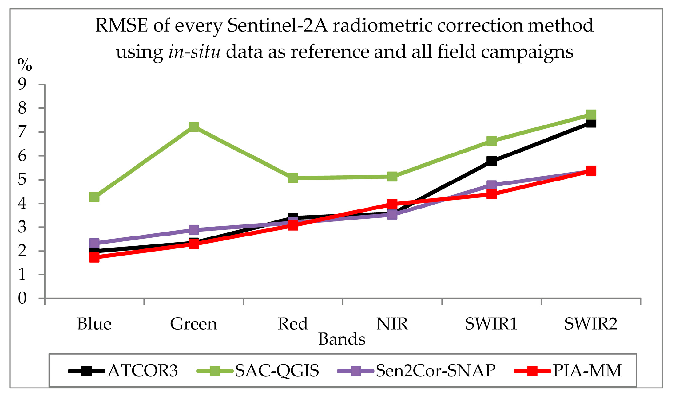
3.2. Results for the Sentinel Platform

The Sentinel-2A imagery acquired on 20 May 2016 showed an excellent fit, with in-situ measurements for all of the methods. Sen2cor-SNAP yielded the highest r² for the blue, green, and red bands (0.999, 0.998, 0.999), SAC-QGIS for the NIR band (0.988), ATCOR3 for the SWIR2 band (0.945), and ATCOR3 and PIA-MiraMon showed the same r² for the SWIR1 band (0.969). When all of the bands were grouped together, PIA-MiraMon yielded the best r² (0.966), followed by Sen2cor-SNAP (0.961). ATCOR3 (0.960) agreement was very close to the Sen2cor-SNAP results, and finally SAC-QGIS (0.939) yielded the lowest agreement with in-situ data (

Table 5. Band-by-band coefficient of determination (r²) between field spectroradiometry values and atmospheric corrections for Sentinel-2A (MSI) imagery. Best values in bold.

Field vs. Sentinel-2A		Blue r2	Green r2	Red r2	NIR r2	SWIR1 r2	SWIR2 r2	All Bands r2
May 2016	ATCOR3	0.987	0.981	0.978	0.987	0.969	0.945	0.960
	SAC-QGIS	0.994	0.997	0.998	0.988	0.967	0.943	0.939
	Sen2Cor-SNAP	0.999	0.998	0.999	0.986	0.968	0.942	0.961
	PIA-MM	0.994	0.997	0.997	0.987	0.969	0.944	0.966
October 2016	ATCOR3	0.995	0.994	0.996	0.955	0.975	0.982	0.952
	SAC-QGIS	0.989	0.975	0.986	0.952	0.971	0.982	0.886
	Sen2Cor-SNAP	0.986	0.970	0.983	0.951	0.970	0.981	0.963
	PIA-MM	0.986	0.972	0.984	0.950	0.972	0.983	0.958
April 2017	ATCOR3	0.911	0.920	0.902	0.982	0.991	0.907	0.942
	SAC-QGIS	0.922	0.917	0.915	0.983	0.988	0.985	0.907
	Sen2Cor-SNAP	0.916	0.913	0.915	0.984	0.989	0.986	0.948
	PIA-MM	0.922	0.917	0.914	0.982	0.985	0.983	0.897
June 2017	ATCOR3	0.925	0.931	0.929	0.992	0.970	0.953	0.953
	SAC-QGIS	0.979	0.982	0.991	0.991	0.967	0.952	0.939
	Sen2Cor-SNAP	0.992	0.991	0.995	0.992	0.968	0.953	0.961
	PIA-MM	0.979	0.982	0.992	0.992	0.968	0.953	0.932

).

Sentinel-2A imagery that was acquired on 4 October 2016 showed a good fit, with in-situ measurements for all of the bands and for all the methodologies. ATCOR3 yielded the highest r² for the blue, green, red, NIR, and SWIR1 bands (0.995, 0.994, 0.996, 0.955, 0.975), while for the SWIR2 band, PIA-MiraMon had the highest (0.983). When all of the bands were grouped together, Sen2Cor-SNAP had the best r² (0.963), followed by PIA-MiraMon (0.958), ATCOR3 (0.952), and SAC-QGIS (0.886) obtained the lowest fit to in-situ data (Table 5).

Sentinel-2A imagery acquired on 22 April 2017 showed a good fit with in-situ measurements for all of the bands and for all methodologies. ATCOR3 showed the highest r² for the green and SWIR1 bands (0.920, 0.991), Sen2Cor-SNAP for the NIR and SWIR2 bands (0.984, 0.986), followed by the PIA-MiraMon method for the blue band (0.922) and SAC-QGIS for the red band (0.915). When all of the bands were grouped together, Sen2Cor-SNAP had the best r² (0.948), followed by ATCOR (0.942), SAC-QGIS (0.907), and PIA-MiraMon (0.897) (Table 5).

Sentinel-2A imagery that was acquired on 1 June 2016 showed a good fit to in-situ measurements for all the bands and for all of the methodologies. Sen2Cor-SNAP yielded the highest r² for the blue, green and red bands (0.992, 0.991, 0.995), tying with ATCOR3 and PIA-MiraMon in the NIR and SWIR2 bands (0.992, 0.953). When all the bands were grouped together, Sen2Cor-SNAP again showed the best r² (0.961), followed by ATCOR3 (0.953), SAC-QGIS (0.939), and PIA-MiraMon (0.932) (Table 5).

The p-value of all the bands and methods is <0.01. Figure 10 shows the correlations between field data and its corresponding pixels of Sentinel-2 imagery corrected with each method and each month, grouping all of the bands.

In terms of the differences in reflectance values of all methods used for Sentinel-2A images, the PIA-MiraMon radiometric correction had the lowest RMSE values in four out of six bands (visible bands (1.727, 2.284, 3.070) and SWIR1 (4.383)), the Sen2Cor-SNAP official product provided the best result in NIR and SWIR2 (3.519, 5.352), and ATCOR3 obtained better results in NIR (3.569) then PIA-MiraMon. PIA-MiraMon had the best result for all of the band averages (3.468) (

Table 6. Overall, band-by-band RMSE between field spectroradiometry values and atmospheric corrections for Sentinel-2A (MSI) imagery (% reflectance units) grouping all dates. Best values in bold.

Field vs. Sentinel-2A	Blue RMSE	Green RMSE	Red RMSE	NIR RMSE	SWIR1 RMSE	SWIR2 RMSE	Mean RMSE
ATCOR3	1.991	2.339	3.381	3.569	5.772	7.393	4.074
SAC-QGIS	4.262	7.217	5.068	5.129	6.621	7.736	6.006
Sen2Cor-SNAP	2.317	2.881	3.190	3.519	4.764	5.352	3.671
PIA-MM	1.727	2.284	3.070	3.973	4.383	5.370	3.468

and Figure 11).

The analysis of the band-by-band behaviour of the PIA-MiraMon method for Sentinel-2A imagery (Table 5) shows that r² also yields a good agreement. There is no band where PIA-MiraMon fails when Sentinel-2A imagery is corrected. Moreover, when the RMSE is considered (Table 6), PIA-MiraMon obtains the lowest differences with respect to the in-situ data in all of the bands, except for NIR and SWIR2.

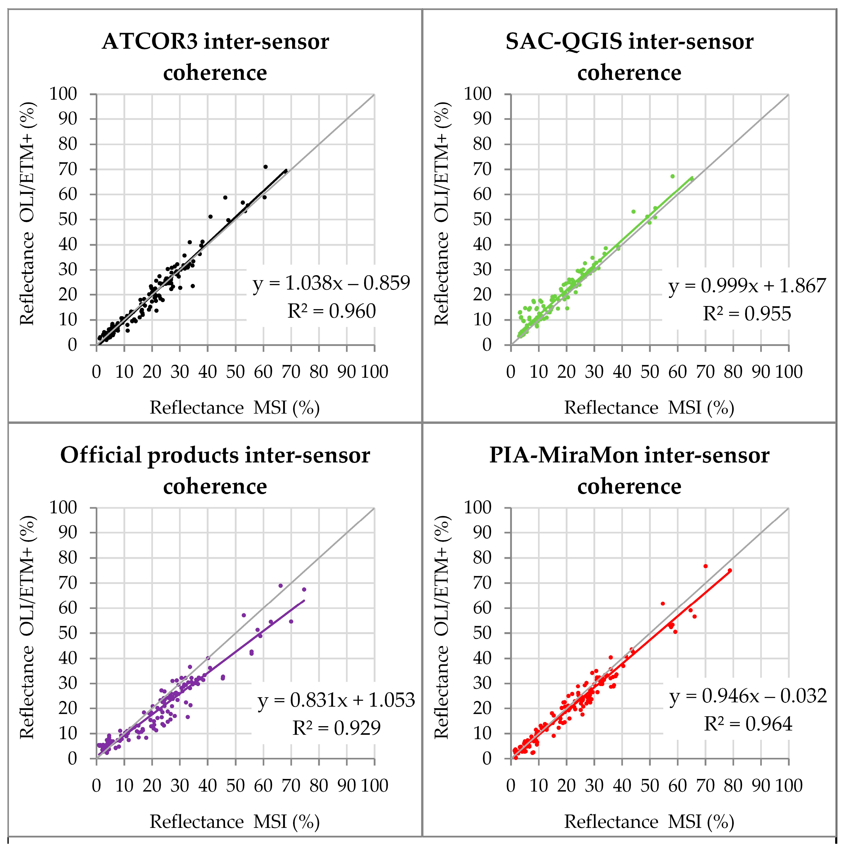
3.3. Inter-Sensor Coherence

Correlation of Landsat and Sentinel-2A images that were acquired almost at the same time, and corrected with the same method (except for the official products (6S-LEDAPS/6S-LaSRC and Sen2Cor-SNAP)), showed the best coefficient of determination (r²) for PIA-MiraMon in the blue, green, and red bands (0.916, 0.961, 0.966), for SAC-QGIS in the SWIR1 and SWIR2 bands (0.982, 0.972), and for ATCOR3 in NIR band (0.986) (

Table 7. Band-by-band coefficient of determination (r²) between simultaneous Landsat (ETM+ and OLI) and Sentinel-2A (MSI) radiometrically corrected images. Correlated values are sampled pixels. Best values in bold.

Sentinel-2A vs. Landsat		Blue r2	Green r2	Red r2	NIR r2	SWIR1 r2	SWIR2 r2	All Bands r2
ALL DATES	ATCOR3	0.908	0.916	0.927	0.986	0.979	0.927	0.960
	SAC-QGIS	0.298	0.799	0.928	0.981	0.982	0.972	0.955
	Official products	0.901	0.939	0.931	0.976	0.976	0.967	0.929
	PIA-MM	0.916	0.961	0.966	0.972	0.975	0.970	0.964

). When all of the bands were grouped together, the best r² was found when the PIA-MiraMon method (0.964) was used, followed by ATCOR3 (0.960), SAC-QGIS (0.955), and the official products (0.929), as seen in Figure 12.

4. Discussion

Analyzing the coeffecient of determination (r²) results that are described above, we find that the PIA-MiraMon radiometric correction method showed a very good fit with field data for all of the bands. Only in seven out of the 48 analyses (6 bands × 4 dates × 2 platforms) did PIA-MiraMon yield the lowest r² value, but it is worth noting that, in these cases, the difference with the next worst method is only around 0.007 points. In 15 out of the 48 analyses PIA-MiraMon yielded the highest agreement (in some cases tying with other methods), and in the remaining 26 analyses the performance of PIA-MiraMon is comparable to the other methods.

When r² was calculated using all of the samples for all bands, and for a given sensor and date (last column in Table 3 and Table 5), PIA-MiraMon obtained the highest value in four of the eight cases. The other four best results were obtained when official tools were used (6S-LEDAPS for ETM+, 6S-LaSRC for OLI, and Sen2Cor-SNAP for MSI). Moreover, PIA-MiraMon was the method that performed best in three of the four cases of OLI imagery, and 6S-LEDAPS was the best in the remaining case. Sen2Cor-SNAP was the method that performed best in three of the four cases of MSI imagery, and PIA-MiraMon was the best in the remaining case.

Although the methods that we compared use different approaches and models, the results are not dramatically different, a similar situation also noticed by Song [47] when comparing different atmospheric correction methods for Landsat-5 TM imagery (DOS (4 variants), DDV, Modified DDV (MDDV), path radiance lineal regression (PARA), and linear relationship using PIF), showing very good and similar results for the DOS and PIF approaches. Now, our results over ETM+, OLI, and MSI show that the PIA-based method clearly offers better accuracies than the DOS method. Note that the PIF-based method uses a linear relationship between radiometric references and the image to be corrected, while the PIA-based method uses the radiometric references to fit the best combination of TOD and path radiance values. In consonance with our findings, where physical approaches do not significantly improve the results of radiometric reference approaches, Song concluded that a huge difference in model complexity does not necessary imply the same difference in accuracy.

The difference in the results cannot be explained by the use or not of a DEM because the selected area is absolutely plain, but can be explained by the influence of the atmospheric parameters (atmospheric spectral radiance (Latm_λ) and Total Optical Depth) that are used in each method. That the SAC-QGIS method does not use the TOD seems to be the major source of discrepancy for this method; SAC-QGIS obtains good coefficients of determination, but the RMSE (in reflectance values (%)) is not as good as other methods. ATCOR-based and 6S-based methods use OLI and MSI bands that are located at specific wavelengths to obtain the distribution of aerosol and water-vapor content in the atmosphere, yielding very good results, but it is worth noting that these bands do not exist in ETM+, TM, and MSS sensors, and the same exact method cannot be used for this imagery. The PIA-MiraMon method obtains similar results as the official products by adjusting the atmospheric parameters to a radiometric surface reflectance reference databank. The PIA-MiraMon method obtains good results because it can exclude the PIA that would not keep the reference value in the case of being corrected (due to cloud presence, land cover changes, etc.), while it can adjust the best combination of Latm_λ and TOD in the PIAs that keep the reference value. Moreover, this capability makes it possible to correct images from the present and the past using the same PIA databank. The accurate selection of the most stable pixels of all the MODIS series to obtain the PIA databank is crucial for dealing with trustable radiometric surface reflectance references.

Besides showing a good adjustment to and low differences with field data, PIA-MiraMon obtained the best results in inter-sensor coherence. SAC-QGIS showed a good inter-sensor correlation in infrared bands, but in the reflectance differences (RMSE) to field data, the results were not as reliable as the other methods (PIA-MiraMon, ATCOR3 or official products). The results of the inter-comparison of official products were not unexpected, as the use of different radiometric correction codes, which are specifically adapted to each sensor, provided good outcomes for their corrected imagery, but not the best correlations between inter-sensor data. Vuolo et al. [90] evaluated the Sen2Cor-SNAP and 6S-LaSRC coherence at six european test sites, obtaining an r² = 0.9, similar to the r² = 0.92 obtained in the present study. On the other hand, PIA-MiraMon showed a good inter-sensor correlation (r² = 0.96), providing robustly corrected data, because it is based on common radiometric areas. Note that the SAC-QGIS inter-sensor coherence in the blue and green bands is notably lower than the other methods, a result that can be explained by the assumption of TOD = 1 of SAC-QGIS and to an inaccurate estimation of atmospheric radiance by the DOS method that is specially affecting the spectral regions where atmospheric scattering is more important. Finally, the effects of the different MSI, OLI, and ETM+ RSRF can explain the lower inter-sensor correlations in the blue band for all of the methods (Table 7), since MSI of Sentinel-2A has a significantly lower sensitivity between 460 nm and 520 nm [59] than OLI [58], ETM+ [57], or even the MSI instrument of Sentinel-2B [59] (Figure 5).

5. Conclusions

Field spectroradiometry measurements for different land cover types for four different dates were used to evaluate the performance of the PIA-MiraMon radiometric correction method applied to pairs of Landsat and Sentinel imagery acquired almost simultaneously. The results were also compared with three other radiometric correction methods.

The comparison of field spectroradiometric measurements with simultaneous acquisitions of Landsat-7 (ETM+), Landsat-8 (OLI), and Sentinel-2A (MSI) imagery that was radiometrically corrected using the PIA-MiraMon method yielded good agreement results (r² > 0.9) for the different dates. The results were similar, when not better, to the same field measurements with the imagery radiometrically corrected with other standard products (6S-LaSRC, 6S-LEDAPS, Sen2Cor-SNAP) and widely used methods (ATCOR3, SAC-QGIS).

Specifically, four pairs of images acquired almost simultaneously from two platforms, three pairs of Landsat-8 and Sentinel-2A, and another pair of Landsat-7 and Sentinel-2A were processed. When the RMSE was computed between radiometrically corrected satellite data and field spectroradiometric data for the whole set of Landsat images, PIA-MiraMon yielded superior results for five out of six bands (mean value: 3.484%), while ATCOR3 provided the best results for the NIR band (mean value of all bands: 3.911%). Similarly, the results for Sentinel-2A images also showed that PIA-MiraMon yielded the best results for four out of the six bands (mean value of all bands: 3.468%), while the official Sen2Cor-SNAP provided the best results for the other 2 (NIR and SWIR2) (mean value of all bands: 3.671%).

In general, the results of the methods from the official agencies (6S-LEDAPS, 6S-LaSRC, Sen2Cor-SNAP) showed very good agreement for their own sensors, but general products, especially ATCOR3, also showed very good results for MSI. On average, SAC-QGIS was the method showing least agreement, although it was not far from the other products analyzed.

The inter-sensor comparison has proven the consistency of the PIA-MiraMon method, showing that it provides a coherent correction of images that were acquired almost simultaneously (r² > 0.964); this confirms the robustness of this method when time series involving different sensors are corrected.

In accordance with previous demonstrations of the PIA approach that was used to radiometrically correct long time series [43], it has now been proven that this is a sound method for contributing to the Landsat time series legacy by coherently correcting imagery from the current Landsat continuity instrument (OLI) and a Landsat-like instrument, such as MSI.

In addition to being a reasonably robust and automatic radiometric correction procedure, it is important to highlight that the PIA-based radiometric correction method is capable of correcting pre-MODIS images and/or when no detailed atmospheric data is available, and it provides similar accuracies than other reference solutions. PIA-MiraMon is the Radiometric Correction module that is available in the Professional MiraMon GIS & RS software, running either from command line (CorRad.exe) or from a dialog box in the Tools main menu.

References

1. National Aeronautics and Space Administration (NASA). Landsat Data Continuity Mission (LCDM). Available online: https://www.nasa.gov/mission_pages/landsat/main/index.html (accessed on 28 October 2017).
2. GEOSS. GEOSS Evolution. Available online: http://www.earthobservations.org/geoss.php (accessed on 28 October 2017).
3. European Space Agency (ESA). ESA Sentinel Online. Sentinel-2 Mission. Available online: http://www.esa.int/Our_Activities/Observing_the_Earth/Copernicus/Sentinel-2 (accessed on 28 October 2017).
4. European Space Agency (ESA). ESA Sentinel Online. Sentinel-2 Mission Objectives. Available online: https://sentinel.esa.int/web/sentinel/missions/sentinel-2/mission-objectives (accessed on 28 October 2017).
5. Drusch, M.; Del Bello, U.; Carlier, S.; Colin, O.; Fernandez, V.; Gascon, F.; Hoersch, B.; Isola, C.; Laberinti, P.; Martimort, P.; et al. Sentinel-2: ESA’s Optical High-Resolution Mission for GMES Operational Services. Remote Sens. Environ. 2012, 120, 25–36. [Google Scholar] [CrossRef]
6. Chander, G.; Markham, B.L.; Helder, D.L. Summary of Current Radiometric Calibration Coefficients for Landsat MSS, TM, ETM+, and EO-1 ALI Sensors. Remote Sens. Environ. 2009, 113, 893–903. [Google Scholar] [CrossRef]
7. Barsi, J.A.; Kenton, L.; Kvaran, G.; Markham, B.L.; Pedelty, J.A. The Spectral Response of the Landsat-8 Operational Land Imager (OLI). Remote Sens. 2014, 6, 10232–10251. [Google Scholar] [CrossRef]
8. Mishra, N.; Helder, D.; Barsi, J.; Markham, B. Continuous calibration improvement in solar reflective bands: Landsat 5 through Landsat 8. Remote Sens. Environ. 2016, 1185, 7–15. [Google Scholar] [CrossRef]
9. Czapla-Myers, J.; McCorkel, J.; Anderson, N.; Thome, K.; Bigar, S.; Helder, D.; Aaron, D.; Leigh, L.; Mishra, N. The Ground-Based Absolute Radiometric Calibration of Landsat 8 OLI. Remote Sens. 2015, 7, 600–626. [Google Scholar] [CrossRef]
10. Saunier, S.; Northrop, A.; Lavender, S.; Galli, L.; Ferrara, R.; Mica, S.; Biasutti, R.; Gory, P.; Gascon, F.; Meloni, M.; et al. European Space Agency (ESA) Landsat MSS/TM/ETM+/OLI Archive: 42 Years of our history. In Proceedings of the IEEE 9th International Workshop on the Analysis of Multitemporal Remote Sensing Images (MultiTemp), Brugge, Belgium, 27–29 June 2017. [Google Scholar]
11. Gascon, F.; Bouzinac, C.; Thépaut, O.; Jung, M.; Francesconi, B.; Louis, J.; Lonjou, V.; Lafrance, B.; Massera, S.; Gaudel-Vacaresse, A.; Languille, F.; et al. Copernicus Sentinel-2A Calibration and Products Validation Status. Remote Sens. 2017, 9, 584. [Google Scholar] [CrossRef]
12. CEOS-WGCV. CEOSS Cal/Val Portal. Available online: http://calvalportal.ceos.org/ (accessed on 28 October 2017).
13. Zhang, Z.; He, G.; Wang, X. A practical DOS model-based atmospheric correction algorithm. Int. J. Remote Sens. 2010, 31, 2837–2852. [Google Scholar] [CrossRef]
14. Markham, B.; Barsi, J.; Kvaran, G.; Ong, L.; Kaita, E.; Biggar, S.; Czapla-Myers, J.; Mishra, N.; Helder, D. Landsat-8 Operational Land Imager Radiometric Calibration and Stability. Remote Sens. 2014, 6, 12275–12308. [Google Scholar] [CrossRef]
15. Claverie, M.; Masek, J. Harmonized Landsat-8 Sentinel-2 (HLS) Product’s Guide. v.1.3. 2017. Available online: https://hls.gsfc.nasa.gov/documents/ (accessed on 28 October 2017).
16. Atmospheric Correction Inter-Comparison Exercise (ACIX). Available online: https://earth.esa.int/web/sppa/meetings-workshops/acix (accessed on 28 October 2017).
17. Holben, B.N.; Eck, T.F.; Slutsker, I.; Tanré, D.; Buis, J.P.; Setzer, A.; Vermote, E.; Reagan, J.A.; Kaufman, Y.J.; Nakajima, T.; et al. AERONET—A Federated Instrument Network and Data Archive for Aerosol Characterization. Remote Sens. Environ. 1998, 66, 1–16. [Google Scholar] [CrossRef]
18. Pons, X.; Solé-Sugrañes, L. A simple radiometric correction model to improve automatic mapping of vegetation from multispectral satellite data. Remote Sens. Environ. 1994, 45, 317–332. [Google Scholar] [CrossRef]
19. Kokhanovsky, A.A.; de Leeuw, G. Satellite Aerosol Remote Sensing over Land, 1st ed.; Springer: Berlin/Heidelberg, Germany, 2009; p. 388. [Google Scholar]
20. Liou, K.N. An Introduction to Atmospheric Radiation, 2nd ed.; Academic Press: San Diego, CA, USA, 2002; p. 583. [Google Scholar]
21. Hadjimitsis, D.G.; Clayton, C.R.I.; Retalis, A. The use of selected Pseudoinvariant targets for the application of atmospheric correction in multi-temporal studies using satellite remotely sensed imagery. Int. J. Appl. Earth Obs. Geoinf. 2009, 11, 192–200. [Google Scholar] [CrossRef]
22. Kaufman, Y.J.; Sendra, C. Algorithm for automatic atmospheric corrections to visible and near-IR satellite imagery. Int. J. Remote Sens. 1988, 9, 1357–1381. [Google Scholar] [CrossRef]
23. Chavez, P.S., Jr. An improved dark-object subtraction technique for atmospheric scattering correction of multispectral data. Remote Sens. Environ. 1988, 24, 459–479. [Google Scholar] [CrossRef]
24. Vermote, E.; Justice, C.; Claverie, M.; Franch, B. Preliminary analysis of the performance of the Landsat 8/OLI land surface reflectance product. Remote Sens. Environ. 2016, 185, 46–56. [Google Scholar] [CrossRef]
25. Turner, R.E.; Malila, W.A.; Nalepha, R.F. Importance of atmospheric scattering in remote sensing. In Proceedings of the Seventh International Symposium on Remote Sensing of Environment, Ann Arbor, MI, USA, 17–21 May 1971; Volume 3, pp. 1651–1697. [Google Scholar]
26. Rozanov, V.V.; Rozanov, A.V. User’s Guide for the Software Package SCIATRAN (Radiative Transfer Model and Retrieval Algorithm V.3.5); Institute of Remote Sensing, University of Bremen: Bremen, Germany, 2016; pp. 1–166. Available online: http://www.iup.uni-bremen.de/sciatran/free_downloads/users_guide_sciatran.pdf (accessed on 6 September 2017).
27. Rozanov, A.; Rozanov, V.; Buchwitz, M.; Kokhanovsky, A.A.; Burrows, J.P. SCIATRAN 2.0–A new radiative transfer model for geophysical applications in the 175–2400 nm spectral region. Adv. Space Res. 2005, 36, 1015–1019. [Google Scholar] [CrossRef]
28. Kotchenova, S.Y.; Vermote, E.F.; Matarrese, R.; Klemm, F.J., Jr. Validation of a vector version of the 6S radiative transfer code for atmospheric correction of satellite data. Part I: Path radiance. Appl. Opt. 2006, 26, 6762–6774. [Google Scholar] [CrossRef]
29. Kotchenova, S.Y.; Vermote, E.F. Validation of a vector version of the 6S radiative transfer code for atmospheric correction of satellite data. Part II: Homogeneous Lambertian and anisotropic surfaces. Appl. Opt. 2007, 46, 4455–4464. [Google Scholar] [CrossRef] [PubMed]
30. Stamnes, K.; Tsay, S.-C.; Wiscombe, W.; Jayaweera, K. Numerically stable algorithm for discrete-ordinate-method radiative transfer in multiple scattering and emitting layered media. Appl. Opt. 1988, 27, 2502–2509. [Google Scholar] [CrossRef] [PubMed]
31. Stamnes, K.; Tsay, S.-C.; Wiscombe, W.; Laszlo, I. DISORT, a General-Purpose Fortran Program for Discrete-Ordinate-Method Radiative Transfer in Scattering and Emitting Layered Media: Documentation of Methodology (Version 1.1); Tech. Rep.; Department of Physics and Engineering Physics, Stevens Institute of Technology: Hoboken, NJ, USA, 2000; p. 112. [Google Scholar]
32. Eriksson, P.; Buehler, S.A.; Davis, C.P.; Emde, C.; Lemke, O. ARTS, the atmospheric radiative transfer Simulator, version 2. J. Quant. Spectrosc. Radiat. Transf. 2011, 112, 1551–1558. [Google Scholar] [CrossRef]
33. Scott, N.A.; Chedin, A. A fast line-by-line method for Atmospheric Absorption Computations: The Automatized Atmospheric Absorption Atlas. J. Appl. Meteorol. 1981, 20, 802–812. [Google Scholar] [CrossRef]
34. Berk, A.; Conforti, P.; Kennett, R.; Perkins, T.; Hawes, F.; van den Bosch, J. MODTRAN6: A major upgrade of the MODTRAN radiative transfer code. In Proceedings of the SPIE 9088, Algorithms and Technologies for Multispectral, Hyperspectral, and Ultraspectral Imagery XX, Baltimore, MD, USA, 13 June 2014. [Google Scholar]
35. Mayer, B.; Kylling, A. Technical note: The libRadtran software Package for radiative transfer calculations—Description and examples of use. Atmos. Chem. Phys. 2005, 5, 1855–1877. [Google Scholar] [CrossRef]
36. Kokhanovsky, A.A.; Breon, F.-M.; Cacciari, A.; Carboni, E.; Diner, D.; Di Nicolantonio, W.; Grainger, R.G.; Grey, W.M.F.; Höller, R.; Lee, K.H.; et al. Aerosol remote sensing over land: A comparison of satellite retrievals using different algorithms and instruments. Atmos. Res. 2007, 85, 372–394. [Google Scholar] [CrossRef]
37. Kokhanovsky, A.A. Light Scattering Media Optics. Problems and Solutions, 3rd ed.; Willey-Praxis: Chichester, UK, 2004; p. 320. ISBN 978-3-540-21184-6. [Google Scholar]
38. Kokhanovsky, A.A. Polarization Optics of Random Media, 1st ed.; Springer: Berlin/Heidelberg, Germany, 2003; p. 224. ISBN 978-3-540-42635-6. [Google Scholar]
39. European Space Agency (ESA). ESA Missions. ENVISAT Instruments. SCIAMACHY. Available online: https://earth.esa.int/web/guest/missions/esa-operational-eo-missions/envisat/instruments/sciamachy (accessed on 28 October 2017).
40. Aerosol Robotic Network (AERONET). Aeronet Data Download Tool. Version 3 Direct Sun Algorithm. Available online: https://aeronet.gsfc.nasa.gov/ (accessed on 28 October 2017).
41. Chavez, P.S., Jr. Image-Based Atmospheric Corrections—Revisited and Improved. PE&RS 1996, 62, 1025–1036. Available online: https://www.unc.edu/courses/2008spring/geog/577/001/www/Chavez96-PERS.pdf (accessed on 28 October 2017).
42. Hall, F.G.; Strebel, D.E.; Nickeson, J.E.; Goetz, S.J. Radiometric rectification: Toward a common radiometric response among multidate, multisensor images. Remote Sens. Environ. 1991, 35, 11–27. [Google Scholar] [CrossRef]
43. Pons, X.; Pesquer, L.; Cristóbal, J.; González-Guerrero, O. Automatic and improved radiometric correction of Landsat imagery using reference values from MODIS surface reflectance images. Int. J. Appl. Earth Obs. Geoinf. 2014, 33, 243–254. [Google Scholar] [CrossRef]
44. Vidal-Macua, J.J.; Zabala, A.; Ninyerola, M.; Pons, X. Developing spatially and thematically detailed backdated maps for land cover studies. Int. J. Digit. Earth 2016, 10, 175–206. [Google Scholar] [CrossRef]
45. Smith, G.M.; Milton, E.J. The use of the empirical line method to calibrate remotely sensed data to reflectance. Int. J. Remote Sens. 1999, 20, 2653–2662. [Google Scholar] [CrossRef]
46. Xu, J.-F.; Huang, J.-F. Empirical Line Method Using Spectrally Stable Targets to Calibrate IKONOS Imagery. Pedosphere 2007, 18, 124–130. [Google Scholar] [CrossRef]
47. Song, C.; Woodcock, C.E.; Seto, K.C.; Lenney, M.P.; Macomber, S.C. Classification and Change Detection Using Landsat TM Data: When and How to Correct Atmospheric Effects? Remote Sens. Environ. 2001, 75, 230–244. [Google Scholar] [CrossRef]
48. Richter, R.; Schläpfer, D. Atmospheric/Topographic Correction for Satellite Imagery (ATCOR-2/3 User Guide, Version 9.0.2, March 2016). 2016. Available online: http://www.rese.ch/pdf/atcor3_manual.pdf (accessed on 28 October 2017).
49. Congedo, L. Semi-Automatic Classification Plugin Documentation. Release 5.3.2.1. 2016, pp. 161–164. Available online: https://media.readthedocs.org/pdf/semiautomaticclassificationmanual-v4/latest/semiautomaticclassificationmanual-v4.pdf (accessed on 6 September 2017).
50. Masek, J.; Vermote, E.F.; Saleous, N.E.; Wolfe, R.; Hall, F.G.; Huemmrich, K.F.; Gao, F.; Kutler, J.; Lim, T.-K. LEDAPS Calibration, Reflectance, Atmospheric Correction Preprocessing Code, Version 2. Model Product. Available online: https://daac.ornl.gov/MODELS/guides/LEDAPS_V2.html (accessed on 28 October 2017).
51. United States Geological Survey (USGS). Product Guide. Provisional Landsat 8 Surface Reflectance Code (LaSRC) Product. Version 4.0; Department of the Interior: Reston, VA, USA, 2016; p. 36. Available online: https://landsat.usgs.gov/sites/default/files/documents/lasrc_product_guide.pdf (accessed on 28 October 2017).
52. Richter, R.; Louis, J.; Müller-Wilm, U. [L2A-ATBD] Sentinel-2 Level-2A Products Algorithm Theoretical Basis Document. Version 2.0. 2012, pp. 1–72. Available online: https://earth.esa.int/c/document_library/get_file?folderId=349490&name=DLFE-4518.pdf (accessed on 28 October 2017).
53. United States Geological Survey (USGS). WRS-2 Scene Boundaries (Worldwide). Available online: https://landsat.usgs.gov/sites/default/files/documents/WRS-2_bound_world.kml (accessed on 28 October 2017).
54. European Space Agency (ESA). SENTINEL-2 Relative Orbits. Available online: https://sentinel.esa.int/documents/247904/685211/S2A_rel_orbit_groundtrack_10Sec/57bcb79f-2696-4859-8292-07ac7166e884 (accessed on 28 October 2017).
55. United States Geological Survey (USGS). EarthExplorer Download Tool. Available online: https://earthexplorer.usgs.gov/ (accessed on 28 October 2017).
56. European Space Agency (ESA). Copernicus Open Access Hub. Available online: https://scihub.copernicus.eu/dhus/#/home (accessed on 28 October 2017).
57. United States Geological Survey (USGS). Using the USGS Spectral Viewer. Landsat 7 ETM+. Available online: https://landsat.usgs.gov/sites/default/files/documents/L7_RSR.xlsx (accessed on 28 October 2017).
58. National Aeronautics and Space Administration (NASA). Landsat Science, Spectral Response of the Operational Land Imager In-Band. Available online: http://landsat.gsfc.nasa.gov/preliminary-spectral-response-of-the-operational-land-imager-in-band-band-average-relative-spectral-response/ (accessed on 28 October 2017).
59. European Space Agency (ESA). Sentinel Online, Sentinel-2A Document Library, Sentinel-2AA (S2A-SRF). Available online: https://earth.esa.int/documents/247904/685211/Sentinel-2+MSI+Spectral+Responses/ (accessed on 28 October 2017).
60. United States Geological Survey (USGS). Landsat-8 Data User Handbook. Version 2.0. Available online: https://landsat.usgs.gov/landsat-8-l8-data-users-handbook (accessed on 28 October 2017).
61. European Space Agency (ESA). Sentinel-2A User Handbook. Released 24/07/2015. Rev. 2. Available online: https://sentinels.copernicus.eu/web/sentinel/user-guides/document-library/-/asset_publisher/xlslt4309D5h/content/sentinel-2-user-handbook (accessed on 28 October 2017).
62. National Aeronautics and Space (NASA). Landsat Science, Spectral Response of the Multispectral Scanner System In-Band. Available online: http://landsat.gsfc.nasa.gov/spectral-response-of-the-multispectral-scanner-system-in-band-band-average-relative-spectral-response/ (accessed on 28 October 2017).
63. United States Geological Survey (USGS). Using the USGS Spectral Viewer. Landsat 5 TM. Available online: https://landsat.usgs.gov/sites/default/files/documents/L5_TM_RSR.xlsx (accessed on 28 October 2017).
64. Jiménez, M.; Díaz-Delgado, R. Towards a Standard Plant Species Spectral Library Protocol for Vegetation Mapping: A Case Study in the Shrubland of Doñana National Park. ISPRS Int. J. Geo-Inf. 2015, 4, 2472–2495. [Google Scholar] [CrossRef]
65. De Miguel, E.; Fernández-Renau, A.; Prado, E.; Jiménez, M.; Gutiérrez de la Cámara, O.; Linés, C.; Gómez, J.A.; Martín, A.I.; Muñoz, F. A review of INTA AHS PAF. EARSeL eProc. 2014, 13, 20–29. [Google Scholar] [CrossRef]
66. Jiménez, M.; Díaz-Delgado, R.; Vaughan, P.; De Santis, A.; Fernández-Renau, A.; Prado, E.; Gutiérrez de la Cámara, O. Airborne hyperspectral scanner (AHS) mapping capacity simulation for the Doñana biological reserve scrublands. In Proceedings of the 10th International Symposium on Physical Measurements and Signatures in Remote Sensing, Davos, Switzerland, 12–14 March 2007; Schaepman, M., Liang, S., Groot, N., Kneubühler, M., Eds.; Available online: http://www.isprs.org/proceedings/XXXVI/7-C50/papers/P81.pdf (accessed on 28 October 2017).
67. Hatchell, D.C. (Ed.) Analytical Spectral Devices, Inc. (ASD) Technical Guide, 3rd ed.; Analytical Spectral Devices, Inc.: Boulder, CO, USA, 1999. [Google Scholar]
68. Peña-Martinez, R.; Domínguez Gómez, J.A.; Ruiz-Verdú, A. Mapping of Photosynthetic Pigments in Spanish Reservoirs. In Proceedings of the MERIS User Workshop (ESA SP-549), ESA-ESRIN, Frascati, Italy, 10–13 November 2003. [Google Scholar]
69. Mueller, J.L.; Brown, S.W.; Clark, D.K.; Johnson, B.C.; Yoon, H.; Lykke, K.R.; Flora, S.J.; Feinholz, M.E.; Souaidia, N.; Pietras, C.; et al. Ocean Optics Protocols for Satellite Ocean Color Sensor Validation. In Revision 2 NASA; Fargion, G.S., Mueller, J.L., Eds.; Goddard Space Flight Center: Greenbelt, MD, USA, 2000. [Google Scholar]
70. Milton, E.J.; Schaepmann, M.E.; Anderson, K.; Kneubühler, M.; Fox, N. Progress in field spectroscopy. Remote Sens. Environ. 2009, 113, S92–S109. [Google Scholar] [CrossRef]
71. Meroni, M.; Colombo, R. 3S: A novel program for field spectroscopy. Comput. Geosci. 2009, 35, 1491–1496. [Google Scholar] [CrossRef]
72. Mira, M.; Niclòs, R.; Valor, E.; Pons, X.; Cea, C.; García-Santos, V.; Caselles, D.; Caselles, V. Espectroradiometría de campo del visible al infrarrojo térmico de muestras con características espectrales singulares. In Proceedings of the XVI Congreso de la Asociación Española de Teledetección, Sevilla, Spain, 21–22 October 2015; pp. 213–219. Available online: http://www.aet.org.es/congresos/xvi/XVI_Congreso_AET_actas.pdf (accessed on 28 October 2017).
73. Zhu, X.; Liu, D.; Chen, J. A new geostatistical approach for filling gaps in Landsat ETM+ SLC-off images. Remote Sens. Environ. 2012, 124, 49–60. [Google Scholar] [CrossRef]
74. Chen, J.; Zhu, X.; Vogelmann, J.E.; Gao, F.; Jin, S. A simple and effective method for filling gaps in Landsat ETM+ SLC-off images. Remote Sens. Environ. 2011, 115, 1053–1064. [Google Scholar] [CrossRef]
75. Mueller-Wilm, U. Sen2Cor Configuration and User Manual V2.4; European Space Agency: Paris, Frence, 2017; pp. 1–53. Available online: http://step.esa.int/thirdparties/sen2cor/2.4.0/Sen2Cor_240_Documenation_PDF/S2-PDGS-MPC-L2A-SUM-V2.4.0.pdf (accessed on 28 October 2017).
76. Pflug, B. Sentinel-2 L2A Processor Sen2Cor. In Proceedings of the EUFAR/ESA Expert Workshop on Atmospheric Correction of Remote Sensing Data, Berlin, Germany, 26–28 October 2016. [Google Scholar]
77. Instituto Geográfico Nacional. Plan Nacional de Ortofotografía aérea. Modelos Digitales del Terreno Obtenidos a Partir de Nubes de Puntos LIDAR. Available online: http://centrodedescargas.cnig.es/CentroDescargas/index.jsp (accessed on 28 October 2017).
78. NASA Jet Propulsion Laboratory (JPL). NASA Shuttle Radar Topography Mission United States 1 Arc Second; Version 3; NASA EOSDIS Land Processes DAAC, USGS Earth Resources Observation and Science (EROS) Center: Sioux Falls, SD, USA, 2013. Available online: https://lpdaac.usgs.gov (accessed on 28 October 2017).
79. Moran, M.; Jackson, R.; Slater, P.; Teillet, P. Evaluation of simplified procedures for retrieval of land surface reflectance factors from satellite sensor output. Remote Sens. Environ. 1992, 41, 169–184. [Google Scholar] [CrossRef]
80. Hale, S.R.; Rock, B.N. Impact of topographic normalization on land-cover classification accuracy. Photogram. Eng. Remote Sens. 2003, 69, 785–791. [Google Scholar] [CrossRef]
81. Chance, C.M.; Hermosilla, T.; Coops, N.C.; Wulder, M.A.; White, J.C. Effect of topographic correction on forest change detection using spectral trend analysis of Landsat pixel-based composites. Int. J. Appl. Earth Obs. Geoinf. 2016, 44, 186–194. [Google Scholar] [CrossRef]
82. Vermote, E.F.; Tanre, D.; Deuzé, J.L.; Herman, M.; Morcrette, J.-J. Second Simulation of the Satellite Signal in the Solar Spectrum, 6S: An Overview. IEEE Trans. Geosci. Remote Sens. 1997, 35, 675–686. [Google Scholar] [CrossRef]
83. Feng, M.; Huang, C.; Channan, S.; Vermote, E.F.; Masek, J.G.; Townshend, J.R. Quality assessment of Landsat surface reflectance products using MODIS data. Comp. Geosci. 2012, 38, 9–22. [Google Scholar] [CrossRef]
84. Feng, M.; Sexton, J.; Huang, C.; Masek, J.; Vermote, E.F.; Gao, F.; Narasimhan, R.; Channan, S.; Wolfe, R.E.; Townshend, J.R. Global surface reflectance products from Landsat: Assessment using coincident MODIS observations. Remote Sens. Environ. 2013, 134, 276–293. [Google Scholar] [CrossRef]
85. Vermote, E.F.; Kotchenova, S. Atmospheric correction for the monitoring of land surfaces. J. Geophys. Res. Atmos. 2008, 113, 2156–2202. [Google Scholar] [CrossRef]
86. Pons, X. MiraMon. Geographical Information System and Remote Sensing Software, Version 8.01b; Centre for Ecological Research and Forestry Applications (CREAF). Bellaterra. 2004. Available online: http://www.creaf.uab.cat/miramon/Index_usa.htm (accessed on 28 October 2017).
87. Pesquer, L.; Domingo, C.; Pons, X. A Geostatistical Approach for Selecting the Highest Quality MODIS Daily Images. In Proceedings of the Pattern Recognition and Image Analysis: 6th Iberian Conference, IbPRIA 2013, Funchal, Madeira, Portugal, 5–7 June 2013; pp. 608–615. [Google Scholar]
88. Marcello, J.; Eugenio, F.; Perdomo, U.; Medina, A. Assessment of Atmospheric Algorithms to Retrieve Vegetation in Natural Protected Areas Using Multispectral High Resolution Imagery. Sensors 2016, 60, 1624. [Google Scholar] [CrossRef] [PubMed]
89. Feilhauer, H.; Thonfeld, F.; Faude, U.; He, K.S.; Rocchini, D.; Schmidtlein, S. Assessing floristic composition with multispectral sensors—A comparison based on monotemporal and multiseasonal field spectra. Int. J. Appl. Earth Obs. Geoinf. 2013, 21, 218–229. [Google Scholar] [CrossRef]
90. Vuolo, F.; Zółtak, M.; Pipitone, C.; Zappa, L.; Wenng, H.; Immitzer, M.; Weiss, M.; Baret, F.; Atzberger, C. Data Service Platform for Sentinel-2 Surface Reflectance and Value-Added Products: System Use and Examples. Remote Sens. 2017, 8, 938. [Google Scholar] [CrossRef]
Figure 1. Study area: Doñana National Park in green (Spain, EU), Villanueva de los Castillejos sub-area (1), and Laguna de Santa Olalla sub-area (2). Also shown, Landsat (blue outline) [53] and Sentinel (red outline) scenes [54]. Location map in SW Europe with Sentinel-2 R037 orbit (yellow) and R137 orbit (purple).
Remotesensing 09 01319 g001
Figure 2. (Left) Landsat L1T images used. False color composite image (L7 RGB 543, L8 RGB 654); (a) 20 May 2016 (OLI) 203034; (b) 4 October 2016 (OLI) 202034; (c) 22 April 2017 (ETM+) 202034; (d) 1 June 2017 (OLI) 202034. (Right) Sentinel-2A L1C images used. False color composite image (S2 RGB 11·8·4); (e) 20 May 2016 T29SPB; (f) 4 October 2016 T29SQB; and, (g) 22 April 2017 T29SQB. (h) 1 June 2017 T29SQB.
Remotesensing 09 01319 g002
Figure 3. (a) Sampling footprint; (b) Shallow lake water (DG, 1 June 2017); (c) Sand dune (DG, 1 June 2017); (d) Albero (DA, 20 May 2016); (e) Grassland (DA, 20 May 2016); and, (f) Shrub (DG, 1 June 2017).
Remotesensing 09 01319 g003
Figure 4. (a,b) Sampling points near Villanueva de los Castillejos; (c) Sampling points near Laguna Santa Olalla.
Remotesensing 09 01319 g004
Figure 5. Relative Spectral Response Function (RSRF) of blue, green, red, NIR, SWIR1, and SWIR2 matching bands on MSI instrument in Sentinel-2A, OLI instrument in Landsat-8 and ETM+ instrument in Landsat-7.
Remotesensing 09 01319 g005
Figure 6. Geometric procedure used to compare pixels of Landsat-8 OLI (30 m) and Sentinel-2A MSI (20 m and 10 m) with field data plots of 20 m of diameter: 30 m and 20 m pixels are resampled to 10 m and the 20 m of diameter of plot area covers up to 9 pixels. The area that is intersected by the circle in each affected pixel is used to compute its contribution (weight) to the final reflectance value to be compared to the field radiometry.
Remotesensing 09 01319 g006
Figure 7. General workflow, for a given date, of radiometric correction methods and their comparison with field spectroradiometry data.
Remotesensing 09 01319 g007
Figure 8. Scatterplots of the correlation between field measurements (X axis) and the values of its corresponding pixel in each each Landsat atmospheric correction method (Y axis) accounting for all bands (last column in Table 3).
Remotesensing 09 01319 g008
Figure 9. Band-by-band Root Mean Square Error of each radiometric correction method analyzed for Landsat images, grouping all dates.
Remotesensing 09 01319 g009
Figure 10. Scatterplots of the correlation between field measurements (X axis) and the values of its corresponding pixel in each Sentinel-2 atmospheric correction method (Y axis) accounting for all the bands (last column in Table 5).
Remotesensing 09 01319 g010
Figure 11. Band-by-band Root Mean Square Error of each radiometric correction method analyzed for Sentinel-2A images, grouping all dates.
Remotesensing 09 01319 g011
Figure 12. Correlation of Landsat and Sentinel-2A images corrected with the same method (except for official products) evaluating the pixels sampled with field measurements (n = 156).
Remotesensing 09 01319 g012