High Spatial Resolution Visual Band Imagery Outperforms Medium Resolution Spectral Imagery for Ecosystem Assessment in the Semi-Arid Brazilian Sertão

Abstract

Semi-arid ecosystems play a key role in global agricultural production, seasonal carbon cycle dynamics, and longer-run climate change. Because semi-arid landscapes are heterogeneous and often sparsely vegetated, repeated and large-scale ecosystem assessments of these regions have to date been impossible. Here, we assess the potential of high-spatial resolution visible band imagery for semi-arid ecosystem mapping. We use WorldView satellite imagery at 0.3–0.5 m resolution to develop a reference data set of nearly 10,000 labeled examples of three classes—trees, shrubs/grasses, and bare land—across 1000 km${}^2$ of the semi-arid Sertão region of northeast Brazil. Using Google Earth Engine, we show that classification with low-spectral but high-spatial resolution input (WorldView) outperforms classification with the full spectral information available from Landsat 30 m resolution imagery as input. Classification with high spatial resolution input improves detection of sparse vegetation and distinction between trees and seasonal shrubs and grasses, two features which are lost at coarser spatial (but higher spectral) resolution input. Our total tree cover estimates for the study area disagree with recent estimates using other methods that may underestimate treecover because they confuse trees with seasonal vegetation (shrubs and grasses). This distinction is important for monitoring seasonal and long-run carbon cycle and ecosystem health. Our results suggest that newer remote sensing products that promise high frequency global coverage at high spatial but lower spectral resolution may offer new possibilities for direct monitoring of the world’s semi-arid ecosystems, and we provide methods that could be scaled to do so.

1. Introduction

Approximately 2 billion people live in the semi-arid regions of the world—agro-ecological zones characterized by low-to-medium rainfall (∼600 mm per year) typically confined to one rainy season [1]. These ecosystems are critical to planetary health for several reasons. First, more than 600 million people in the semi-arid tropics are smallholder farmers and pastoralists, living on a few hectares of land, at most. These populations, who are among the world’s poorest, depend primarily on rain-fed agriculture for their livelihoods (for cultivation of cereals, forage for livestock, and more). Even small changes in precipitation in these regions may lead to changes in vegetation, which ultimately have important consequences for human welfare, subsequent land cover and land use change—including deforestation (for example, when farmers must expand their land footprint to meet basic needs), and climate change. Second, in steady-state, vegetation in the world’s semi-arid regions is a main driver of the seasonal carbon cycle. Moreover, because these regions often have a larger percentage of precipitable water from vegetation, vegetation and rainfall (and, by extension, human livelihoods) are more tightly coupled than in other ecosystems, and in a potential positive feedback loop [2,3,4]. Over recent decades, semi-arid zones have seen—and are expected to see in the future—larger climate signals compared to the global mean, in part due to this feedback [5,6,7]. As such, the world’s semi-arid regions sit at the nexus of climate impacts, adaptation, food security, and economic development. Monitoring vegetation and biomass dynamics in these regions is critical for a sustainable development.

Ecosystem assessment—or the mapping of the landcover and services provided by a given ecosystem—has traditionally been difficult and costly even locally, and impossible at a global scale or at high temporal resolution. Though remotely sensed data have offered new possibilities for mapping landcover and landuse, until very recently, satellite instruments—especially those that are publicly available—prioritized spectral information (higher radiometric sensitivity) over increased spatial and temporal resolution, in part due to data requirements and computational limitations. Satellite data have been critical to monitoring the world’s dense forests [8], but has been limited in its applicability for monitoring more sparsely-vegetated and heterogeneous landscapes, where key features (e.g., individual trees) are too small to be identified as individual objects by the satellite’s sensors. In the world’s drylands, for example, coarse spatial resolution data has limited our ability to understand the meaning of changes in overall ‘greenness’ [9]; at the same time, higher spatial resolution data may not fully leverage meaningful spectral information about the reflectance of the land cover and is often difficult to scale [10]. Existing and proposed devices, however, like small satellite flocks and coordinated unmanned aerial vehicles (UAV) flights, promise frequent coverage at high spatial but lower spectral resolution (typically the visible red, green, and blue (RGB) bands, and possibly RGB together with near infrared (RGB + NIR)). With the reduced cost of computing, including through analysis on cloud-based platforms like Google Earth Engine, there are new possibilities for monitoring the world’s semi-arid ecosystems on a global seasonal scale.

In light of both the importance of semi-arid ecosystems and the increased availability of high-resolution data and computational capabilities, we seek to answer three related questions here: (1) How well do classifiers based on high-spatial/low-spectral (HSLS) resolution imagery as input perform in classifying the land cover of semi-arid ecosystems, compared to classifiers based on more conventional medium-spatial- resolution input traditionally used for long-run monitoring, like Landsat? (2) Given the importance of the seasonal vegetation cycle in semi-arid regions to both human livelihoods and climate, does HSLS resolution imagery offer a potential source for seasonal carbon cycle information? Finally, (3) can HSLS resolution imagery be used effectively for ecosystem assessment in the heterogeneous and often sparsely vegetated landscapes of the semi-arid tropics? How do large-scale estimates of land cover based on these methods compare with other existing methods?

We evaluate the potential of high-resolution satellite imagery for ecosystem assessment in the case study of the Sertão, a semi-arid biome of northeastern Brazil. In the Sertão, we identified ten 100 km${}^2$ regions representative of the regional landscape heterogeneity. In each region, we performed a 3-class classification into three types of land cover—trees, shrubs, and bare land—using WorldView-2, WorldView-3 and Landsat-8 satellites imagery (representing high- and medium- spatial resolution imagery—or 0.3–0.5 m and 30 m, respectively). These three coarse classes represent the types of landcover that an ecosystem assessment would want to track—bare land as indicative of degraded habitat, shrubs as a broad category of non-tree and largely seasonal vegetation, and trees. We then compared the accuracy of classification with the two sets of imagery as input to the classifiers (WorldView and Landsat), along with several combinations between the sets of inputs. We also tested performance in 2-class classification tasks, as well as in classification across seasons. Our paper proceeds as follows: Section 2 describes the satellite imagery used, construction of the reference data sets, and the methods we used for classification in Google Earth Engine and for cross-validation; Section 3 describes the results, also in the context of seasonal variations; in Section 4, we offer a concluding discussion; we compare our whole-area estimates to existing estimates based on other methods and provide a discussion of the potential to scale our methods to a global, seasonal ecosystem assessment.

2. Materials and Methods

2.1. Overview

Various machine-learning approaches (e.g., supervised, unsupervised and semi-supervised) can be combined with satellite imagery for ecosystem land cover classification, but accurate classification of distinct types of biomes remains challenging due to several constraints. First, there is a scarcity of reference data to facilitate training of classifiers or for validation of existing maps. Second, distinguishing between types of biomes and assessing their health, requires “good enough” satellite imagery. The definition of “good enough”—i.e., the optimal spatial and spectral characteristics of the imagery necessary for classification—remains unspecified. For example, very high-resolution imagery provided by private commercial companies is expensive, and prohibitively so at the global scale. On the other hand, publicly available global-scale satellite imagery is generally characterized by a lower spatial resolution (but by a higher spectral resolution compared to the former). Third, mapping ecosystems on global scales requires overcoming computational constraints (i.e., storage and analysis) which, until recently, with the emergence of cloud based computational platforms such as Google Earth Engine, have limited the scale of the analyzed regions.

In this study, we performed supervised pixel-based image classification of ecosystems in the semi-arid Sertão using an extensive dataset of almost 10,000 examples (points) that were hand-labeled as either trees (within the tree canopy), shrubs (all non-tree vegetation), or land (bare ground). We utilized both medium spatial-resolution imagery (Landsat 8; hereafter referred to as Landsat) and 3-band (RGB) high spatial-resolution imagery (WorldView-2 and WorldView-3; hereafter referred to as WV2 and WV3, respectively). Although the spatial resolution of Landsat is lower than of WorldView (30 m vs. 0.3–0.5 m, respectively), Landsat imagery contains a much wider range spectral information compared to the visible WV imagery (8 vs. 3 spectral bands, respectively), which can be used to calculate other composite spectral indices [11]. Most important, for the purposes of this study, is that the spectrum of 3 of Landsat bands (Bands 2–4 are BGR) overlaps very closely with the spectra of the RGB WorldView bands. This allows us to assess the trade-offs between spatial and spectral resolution in the input data that is used for classification. We perform classification using Landsat and WorldView as separate inputs to the classifiers and using the two inputs combined (where each WorldView pixel also includes Landsat’s band properties). The process is shown visually in Figure 1 and described in detail below.

2.2. Study Area and Region Selection

The Sertão is a semi-arid region in northeast Brazil (Figure 2a). The region, part of the Brazilian Highlands, is characterized by low density vegetation, primarily shrubs and sparse forests. Through a research agreement, we were given access to a subset of WorldView 3-band imagery via the DigitalGlobe Basemap suite (My DigitalGlobe, DigitalGlobe, Inc., Westminster, CO, USA) that included intermittent coverage of parts of the Sertão starting in 2015. We first selected a subset of cloud-free scenes from the available imagery, which narrowed the selection set considerably. Second, to account for the potential seasonal variation known to be present in semi-arid regions, we split our test regions across two seasons—September and March. We did not have access to repeat images of any Sertão locations in the high-resolution imagery spanning two seasons within two calendar years—which would have been ideal in terms of experimental design—and were thus restricted to choosing images from the same year and different locations across seasons. This left us with approximately fifteen 10 km × 10 km regions, from which we selected ten final images (one image per region) spanning the largest area and with the most heterogeneity. These regions represent together a 1000 km${}^2$ area, or a size equivalent to a smaller Brazilian municipality (Figure 2a,b).

2.3. Development of a Reference Training Set

In each region, we randomly sampled 1000 locations (points) to hand-label as reference examples. We overlaid these points on the WorldView imagery and labeled each location as trees, shrubs, or land using two image interpretation approaches: (i) in the first, we labeled examples according to the characteristics of the land cover in the WorldView pixel directly corresponding to the location (referred to as point dataset). In this version, for example, a point is labeled as tree only if it is located precisely over a tree; (ii) in the second approach, we labeled each location according to the majority land cover type in the WorldView imagery within a buffer of 30 m (radius-15 m) around each point (referred to as buffered dataset). In this version, a point is labeled as tree only if more than 50% of the buffer around it is covered with trees. We excluded examples that did not correspond with any of the three classes (i.e., polygons covered with different types of land cover). We pursued this dual labeling strategy to better compare the two different spatial resolutions. Since a Landsat pixel is much larger than a WorldView pixel, directly transferring a label from a fine resolution pixel to a coarse resolution pixel might be misleading (a Landsat pixel will often contain mixed classes). Indeed, the two labeling approaches result in a different distribution of labeled examples: in the point dataset, more examples were labeled as shrubs than trees (51% vs. 28%, respectively), while, in the buffered dataset, fewer examples were labeled as shrubs than trees (40% vs. 46%, respectively) (

Table 1. Distribution of labeled examples by class and tile, for both point and buffer labeling systems (expressed in percentages).

Region	Point Classification			Buffer Classification
	Land	Shrub	Tree	Land	Shrub	Tree
1	5.91	43.04	51.05	4.1	29.73	66.17
2	14.93	27.25	57.82	10.72	23.55	65.73
3	7.71	49.95	42.34	3.6	18.52	77.88
4	8.83	39.92	51.25	5.12	18.96	75.93
5	15.32	48.75	35.94	9.11	24.52	66.37
6	54.21	44.79	1.00	45.69	44.59	9.72
7	37.17	45.49	17.33	33.17	35.17	31.66
8	30.38	62.47	7.14	12.68	70.72	16.6
9	33.67	58.89	7.44	12.96	65.43	21.61
10	6.11	85.67	8.22	1.7	67.94	30.36
Average	21.42	50.62	27.95	13.89	39.91	46.20
Standard Error	5.22	4.97	6.93	4.53	6.61	8.40

presents the distribution of the labeled examples). Twenty-five examples that did not correspond with any of the three classes (e.g., bodies of water or built structure) were not included in our reference dataset. Examples were labeled by three research assistants who were trained extensively and supervised by the research team. Each labeled example is a point, which is associated with exactly one pixel. The classification is thus performed with 9975 labeled pixels (Landsat or WorldView), where each pixel includes inputs (band and indices values) and a response value (a class).

2.4. Classification and Classifier Performance

We performed supervised pixel-based image classification in Google Earth Engine (GEE). GEE leverages cloud-computational services for planetary-scale analysis and consists of petabytes of geospatial and tabular data, including a full archive of Landsat scenes, together with a JavaScript, Python based API (GEE API), and algorithms for supervised image classification [12]. GEE has been previously used for various research applications, including mapping population [13,14], urban areas [15] and forest cover [8].

We used both Landsat and WorldView imagery as input for classification. We matched the selected WorldView regions to the co-located Landsat imagery (8-day TOA reflectance composites) nearest in date, and trimmed Landsat imagery to the same boundaries. We used Landsat 8 Top-of-Atmosphere (TOA) reflectance orthorectified scenes, with calibration coefficients extracted from the corresponding image metadata. The Landsat scenes were from the L1T level product (precision terrain-corrected), converted to TOA reflectance and rescaled to 8-bits for visualization purposes. These pre-processed calibrated scenes are available in GEE. It should be noted that, although TOA reflectance accounts for planetary variations between acquisition dates (e.g., the sun’s azimuth and elevation), many images remain contaminated with haze, clouds, and cloud shadows, which may limit their effective utilization [16], especially for agriculture and ecological applications.

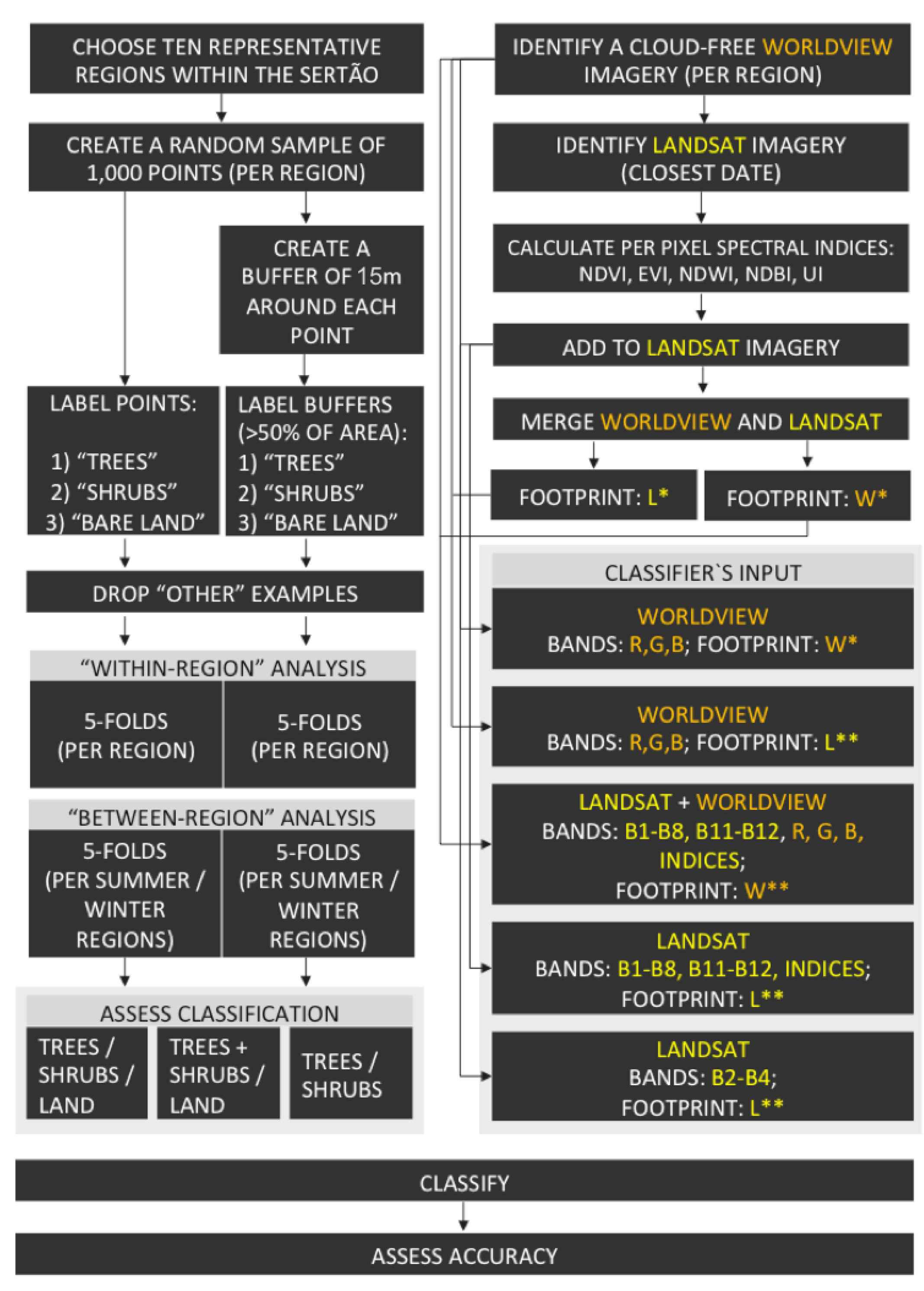
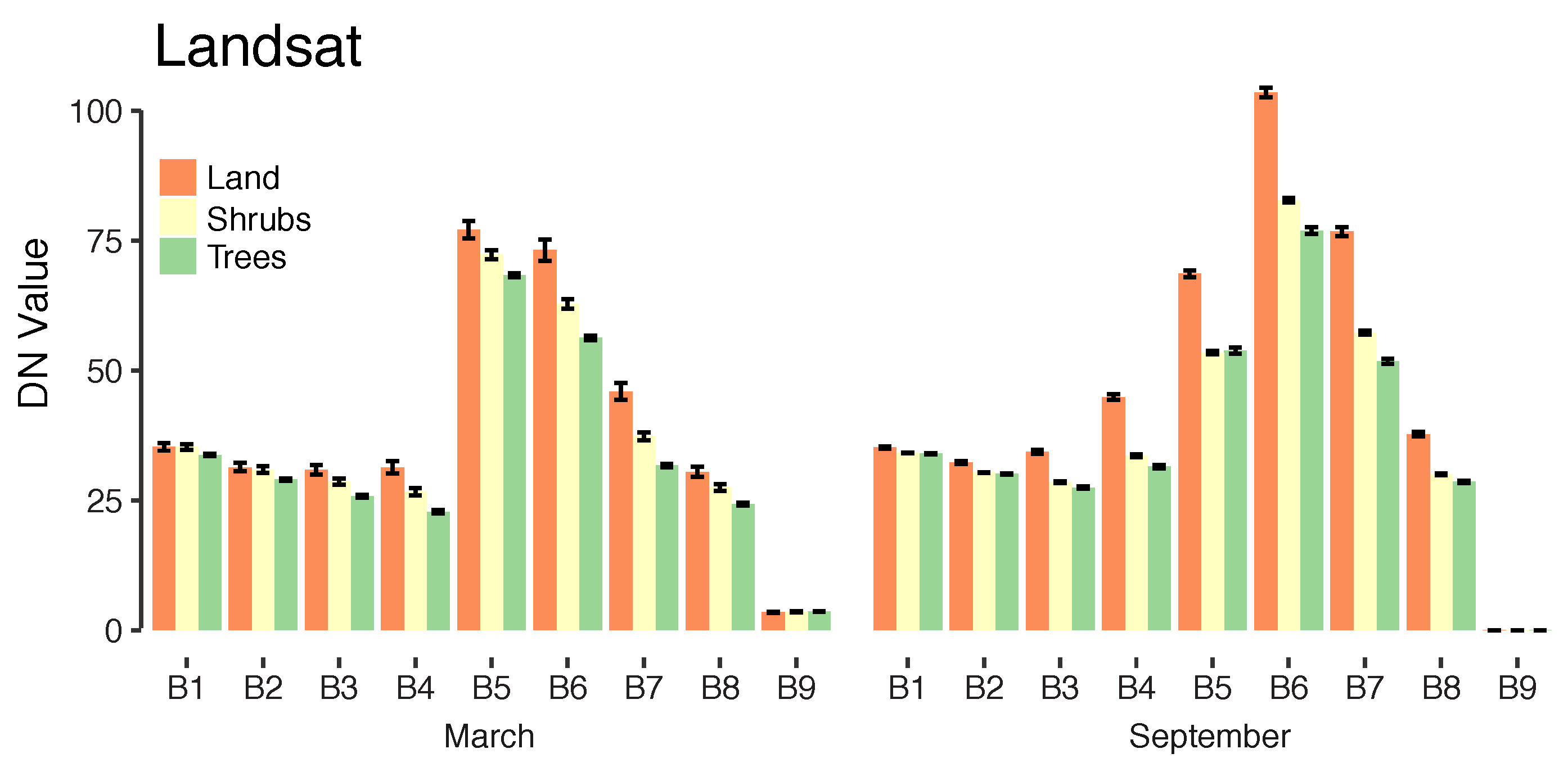
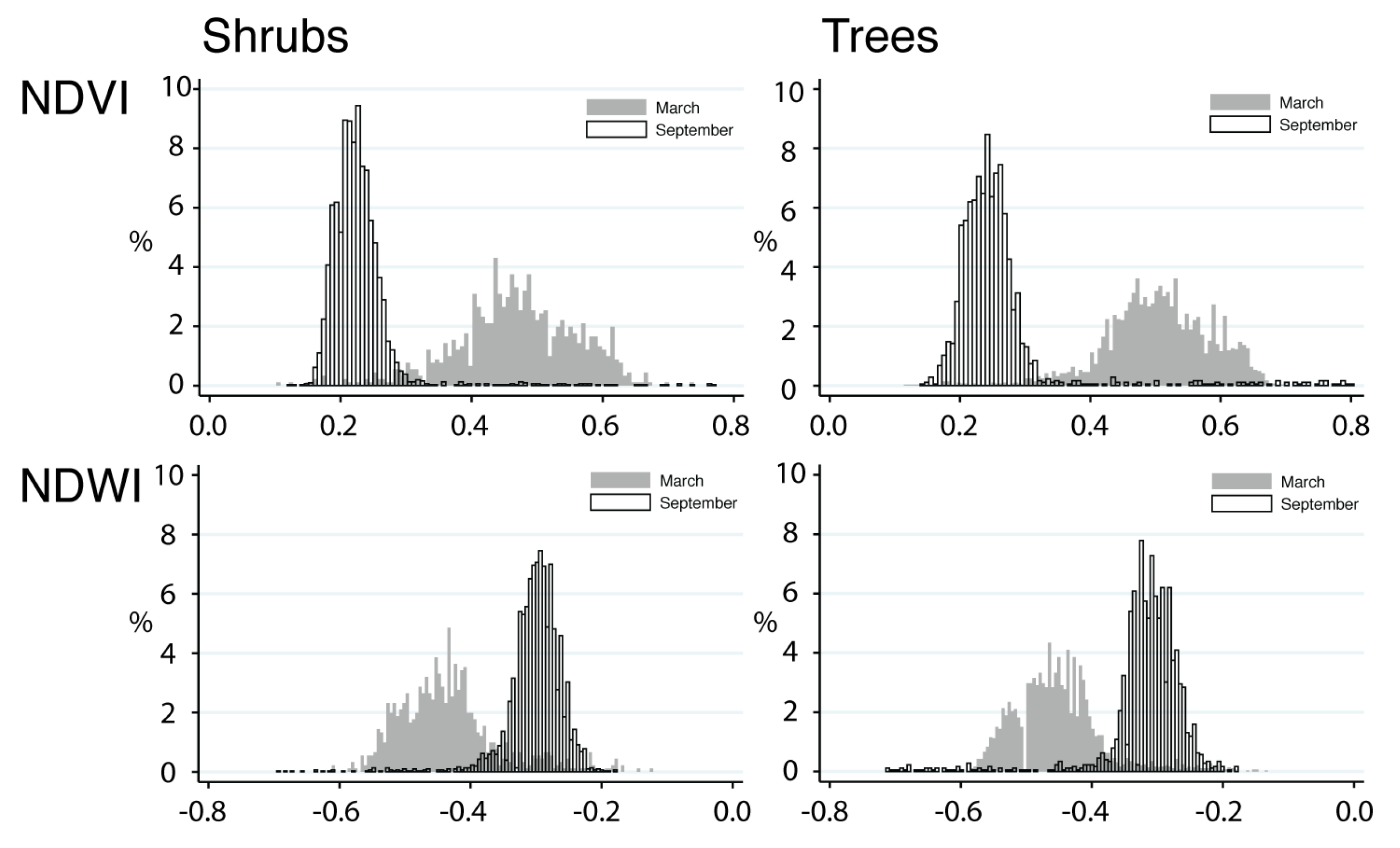
For each Landsat pixel, we used 11 spectral band designations, in a spatial resolution of between 15 m (band 8) to 30 m (bands 1–7, 9–11) and we calculated five spectral indices as additional inputs to the classifier. These indices are commonly used to identify water (Normalized Difference Water Index (NDWI)), built up and bare land areas (Normalized Difference Built-up Index (NDBI); Urban Index (UI)), and vegetation (Normalized Difference Vegetation Index (NDVI); Enhanced Vegetation Index (EVI)). We thus used a total of 15 features per pixel (11 spectral bands and 4 spectral indices). We added these nonlinear indices as additional inputs to the classifier to improve identification of vegetation and bodies of water (NDVI, NDWI and EVI) and other types of land cover (NDBI and UI). Although the latter two indices were originally designed to capture built-up and urban areas, they are also sensitive to the spectral characteristics of bare land [17], which are relatively similar to those of urban areas [18].

For each WorldView pixel, we used 3 spectral band designations (blue, green, and red) in a spatial resolution of 0.5 m (WV2) and 0.3 m (WV3) (bands for WorldView and Landsat are described in

Table A2. Description of spectral bands from Landsat-8 and WorldView-2/WorldView-3 used in classification.

	Spectral Band	Wavelength (micrometers)	Resolution (meters)
Landsat 8
B1	Band 1—Ultra blue	0.43–0.45	30
B2	Band 2—Blue	0.45–0.51	30
B3	Band 3—Green	0.53–0.59	30
B4	Band 4—Đ Red	0.64–0.67	30
B5	Band 5—Near Infrared (NIR)	0.85–0.88	30
B6	Band 6—SWIR 1	1.57–1.65	30
B7	Band 7—SWIR 2	2.11–2.29	30
B8	Band 8—Panchromatic	0.50–0.68	15
B9	Band 9—Cirrus	1.36–1.38	30
B10	Band 10—Thermal Infrared (TIRS) 1	10.60–11.19	100 (resampled to 30)
B11	Band 11—Thermal Infrared (TIRS) 2	11.50–12.51	100 (resampled to 30)
NDVI	(B5 − B4)/(B5 + B4)		30
NDWI	(B3 − B5)/(B3 + B5)		30
NDBI	(B6 − B5)/(B6 + B5)		30
EVI	2.5 * ((B5/B4)/(B5 + 6 * B4 − 7.5 * B2 + 1)		30
UI	(B7 − B5)/(B7 + B5)		30
WorldView 2/3
B	Blue	0.45–0.51	0.5/0.3
G	Green	0.51–0.58	0.5/0.3
R	Red	0.63–0.69	0.5/0.3

). It should be noted that, while WV2 collects imagery at eight multispectral bands (plus Panchromatic) and WV3 collects imagery at eight multispectral bands, eight-band short-wave infrared (SWIR) and 12 CAVIS (plus Panchromatic), we were only granted access to three of WorldView’s imagery bands (the red, green and blue bands). WV2 and WV3 3-band pan sharpened natural color imagery was downloaded from DigitalGlobe Basemap (My DigitalGlobe). The imagery included single-strip ortho with off-nadir angle of 0–30 degrees (the full metadata of the downloaded scenes is presented in Appendix A,

Table A1. Metadata for WorldView imagery used (all scenes are Pan Sharpened Natural Color). Regions correspond to the areas in Figure 2.

Region	Source	Resolution	Date (D/M/Y)	Cloud Cover	Product Type	Off Nadir Angle	Sun Elevation	Sun Azimuth	RMSE Accuracy
1	WV03	30 cm	1/3/16	3.31%	PSNC	12.0392${}^{°}$	67.0268${}^{°}$	86.4171${}^{°}$	3.914
2	WV03	30 cm	1/3/16	3.31%	PSNC	12.0392${}^{°}$	67.0268${}^{°}$	86.4171${}^{°}$	3.914
3	WV03	30 cm	1/3/16	3.31%	PSNC	12.0392${}^{°}$	67.0268${}^{°}$	86.4171${}^{°}$	3.914
4	WV03	30 cm	1/3/16	3.31%	PSNC	12.0392${}^{°}$	67.0268${}^{°}$	86.4171${}^{°}$	3.914
5	WV02	50 cm	13/9/15	0.00%	PSNC	28.7381${}^{°}$	65.2489${}^{°}$	58.3622${}^{°}$	3.914
6	WV02	50 cm	24/9/15	0.00%	PSNC	11.9266${}^{°}$	67.2595${}^{°}$	65.8200${}^{°}$	3.914
7	WV02	50 cm	24/9/15	0.00%	PSNC	11.9266${}^{°}$	67.2595${}^{°}$	65.8200${}^{°}$	3.914
8	WV02	50 cm	11/9/15	0.89%	PSNC	24.6518${}^{°}$	60.8081${}^{°}$	63.9840${}^{°}$	3.914
9	WV02	50 cm	19/9/15	0.18%	PSNC	14.7205${}^{°}$	64.2304${}^{°}$	67.6808${}^{°}$	3.914
10	WV02	50 cm	19/9/15	0.18%	PSNC	14.7205${}^{°}$	64.2304${}^{°}$	67.6808${}^{°}$	3.914

). The WorldView imagery we analyzed was processed by DigitalGlobe. Though temporal analysis with this type of data should be performed with caution (while accounting, for example, for radiometric and atmospheric variations), it is sufficient for the purpose of our study: to evaluate classification performance in one moment of time with different spatial and spectral resolution input data (note that we do not include spectral indices that are based on the WorldView input). Our objective here was not to perform change detection or to classify the land cover in different moments in time. Instead, we performed a basic per-pixel supervised classification procedure, where the characteristics of the feature space (e.g., calibrated or not, DN or reflectance values) are similar in training and classification.

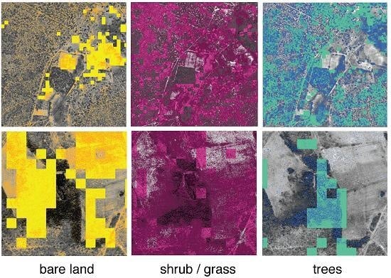
We performed classification with 5 different combinations of inputs to the classifier: using (I) Landsat bands alone (herafter LS8); (II) using WorldView bands alone (hereafter WV); (III) using WorldView bands, rescaled (averaged) to Landsat’s spatial resolution (30 m) (hereafter WV30); (IV) using the subset of 3 Landsat bands, corresponding to WorldView’s visible bands (Red, Green, and Blue) (hereafter LS8RGB); and, finally: (V) using WorldView bands combined with Landsat bands, at the spatial resolution and footprint of WorldView (hereafter WVLS8). The spatial and spectral information for each classifier is summarized in Table A2.

In each case, we used a Random Forest (RF) classifier with 20 decision trees. Random Forests are tree-based classifiers that include k decision trees ( k predictors). When classifying an example, its variables (in this case, spectral bands and/or spectral indices) are run through each of the k tree predictors, and the k predictions are averaged to get a less noisy prediction (by voting on the most popular class). The learning process of the forest involves some level of randomness. Each tree is trained over an independently random sample of examples from the training set and each node’s binary question in a tree is selected from a randomly sampled subset of the input variables. We used RF because previous studies found that the performance of RF is superior to other classifiers [15], especially when applied to large-scale high dimensional data [19]. Random Forests are computationally lighter than other tree ensemble methods [20,21] and can effectively incorporate many covariates with a minimum of tuning and supervision [22], RF often achieve high accuracy rates when classifying hyperspectral, multispectral, and multisource data [23]. In this study, we set the number of trees in the Random Forest classifier to 20. Previous studies have shown mixed results as for the optimal number of trees in the decision tree, ranging from 10 trees [24] to 100 trees [20]. According to [15], although the performance of Random Forest improves as the number of trees increases, this pattern only holds up to 10 trees. Performance remains nearly the same with 50 and with 100 decision trees. Similarly, Du et al. (2015) evaluated the effect of the number of trees (10 to 200) on the performance of RF classifier and showed that the number of trees does not substantially influence the classification accuracy [25]. Because our intention here was not to identify an optimal number of trees in the RF but to compare classification with different types of input, we chose to use a RF classifier with 20 trees and did not imply that this is the optimal number of trees.

In general, automatic classification of land use/land cover (LULC) from satellite imagery can be conducted at the level of a pixel (pixel-based), an object (object-based) or in a combined method. Pixel-based methods for LULC classification rely on the spectral information contained in individual pixels and have been extensively used for mapping LULC, including for change detection analysis [26]. Object-based methods rely on the characteristics of groups of pixels, where pixels are segmented into groups according to similarity and the classification is done per object, rather than per pixel. While several studies suggest that object-based classifiers outperform pixel-based classifiers in LULC classification tasks [27,28,29,30], other studies suggest that pixel-based and object-based classifiers perform similarly when utilizing common machine-learning algorithms [31,32]. In addition, object-based classification requires significantly more computational power than pixel-based classification and there is no universally accepted method to determine an optimal scale level for image segmentation [28], especially when analyzing large-scale and geographically diverse regions. Thus, object-based classification is typically conducted when the unit of analysis is relatively small, such as a city [28,30], or a region of a country [27,30,31,32], as we do in this study. Here, we map land cover at the level of the pixel.

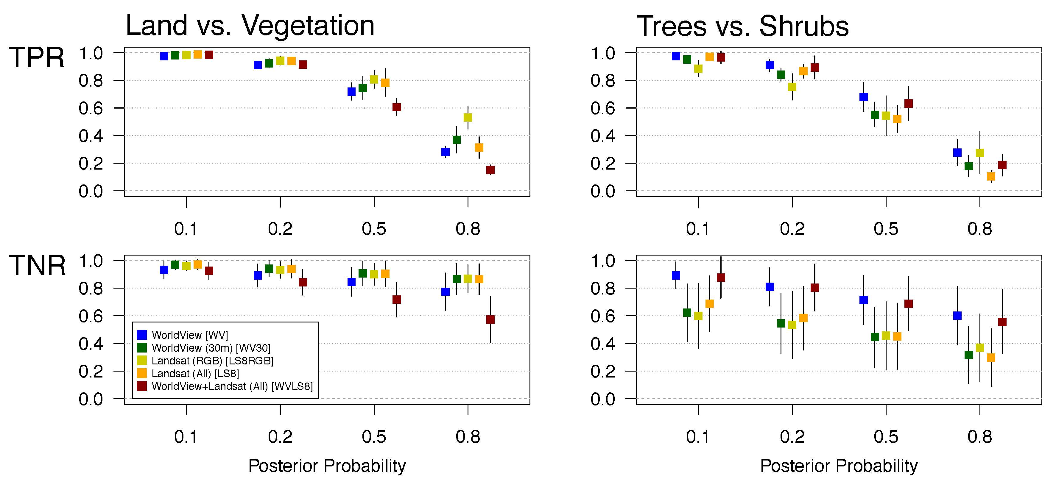
We evaluated the performance of the classifiers in both 3-class classifications, utilizing the full set of examples: trees, shrubs, and land, and 2-class classification, where we classified (I) land versus all vegetation (trees + shrubs) and (II) trees versus shrubs (excluding land). Given a 2-class classification problem (into class C and D), the classifiers predict per-pixel probability of class membership, (posterior probability (p), in the range between 0 and 1) representing the probability that a pixel X belongs to class C (the probability the pixel belongs to class D is 1-p). A pixel X is classified as belonging to class C, if the probability it belongs to class C exceeds a given threshold. An important question in any machine learning task is what is the optimal posterior probability threshold above which a pixel is declared to belong to the ‘positive’ class. To address this question, we also assess performance of 2-class probability-mode classification, where a pixel is declared as positive if the posterior probability exceeds either 0.1, 0.2, 0.5 or 0.8. We evaluate the effect of these posterior probability thresholds on the performance of the classifiers (i.e., the True Positive Rate (TPR) and True Negative Rate (TNR) measures). Although previous studies suggest methods for probability estimates for multi-class classification (i.e., classification into more than two classes), for example, by combining the prediction of multiple or all available pairs of classes [33,34], here we only perform a 2-class probability classification, classifying land versus all vegetation and trees versus shrubs. According to this approach, a pixel is declared as positive (i.e., vegetation or trees, respectively) if the probability it belongs to these classes exceeds a threshold (0.1, 0.2, 0.5 or 0.8). Below this threshold, the pixel is classified as negative (land or shrubs, respectively).

We performed classification of trees versus shrubs only with the examples that were labeled as either one of these two classes. This classification procedure predicts the class of each pixel in the classified universe as either trees or shrubs (although the scenes, by their nature, also include other types of land cover such as bare land). Obviously, mapping this prediction will be misleading, as this is a 2-class classification. In this procedure, each pixel in the universe is classified as one of two classes (trees or shrubs) and the prediction is evaluated against the examples labeled as trees and shrubs in the reference data.

For the 3-class classification, each example (pixel) was classified as one of three classes (trees, shrubs, land), without treating the examples as ‘positive’ or ‘negative’. Given a trained classifier consisting of n trees (in this case 20 trees), each new instance (pixel) is run across all the trees grown in the forest. Each tree predicts the probability an instance belongs to each one of the classes (in this case, one of 3 classes) and votes for the instance’s predicted class. Then, the votes from all trees are combined and the class for which maximum votes are counted is declared as the predicted class of the instance [35,36].

The distinction between classes are all meaningful in an ecological sense, given the landscape heterogeneity and highly varying vegetation patterns of semi-arid regions like the Sertão, and the most appropriate choice of the classified classes depends on the application. For example, a 3-class classification would be most relevant for total ecosystem landcover assessment, whereas land-versus-vegetation would be most relevant for assessing degradation or recovery, and trees-versus-shrubs would be most relevant for assessing seasonal variations in vegetation.

The performance (accuracy) of a classifier refers to the probability that it will correctly classify a random set of examples [37]; the data used to train the classifier must thus be distinct from the data that is used to assess its performance. Labeled (or reference) data is typically divided into training and test sets (a validation set may also be used to “tune” the classifier’s parameters). Different data splitting heuristics can be used to assure a separation between the training and test sets [37], including the holdout method, in which the data is divided into two mutually exclusive subsets: a training set and a test/holdout set; bootstrapping, in which the dataset is sampled uniformly from the data, with replacement; and cross-validation (also known as k-fold cross-validation), in which the data are divided into k subsets, and the classification is performed k times, rotating through each ‘fold’ as a test set. By averaging across the different draws, cross-validation gives a less biased estimate of classifier performance, [38] along with a variance estimation of the classification error [39,40]), but is less computationally intensive than (typically hundreds) of bootstrap re-samples.

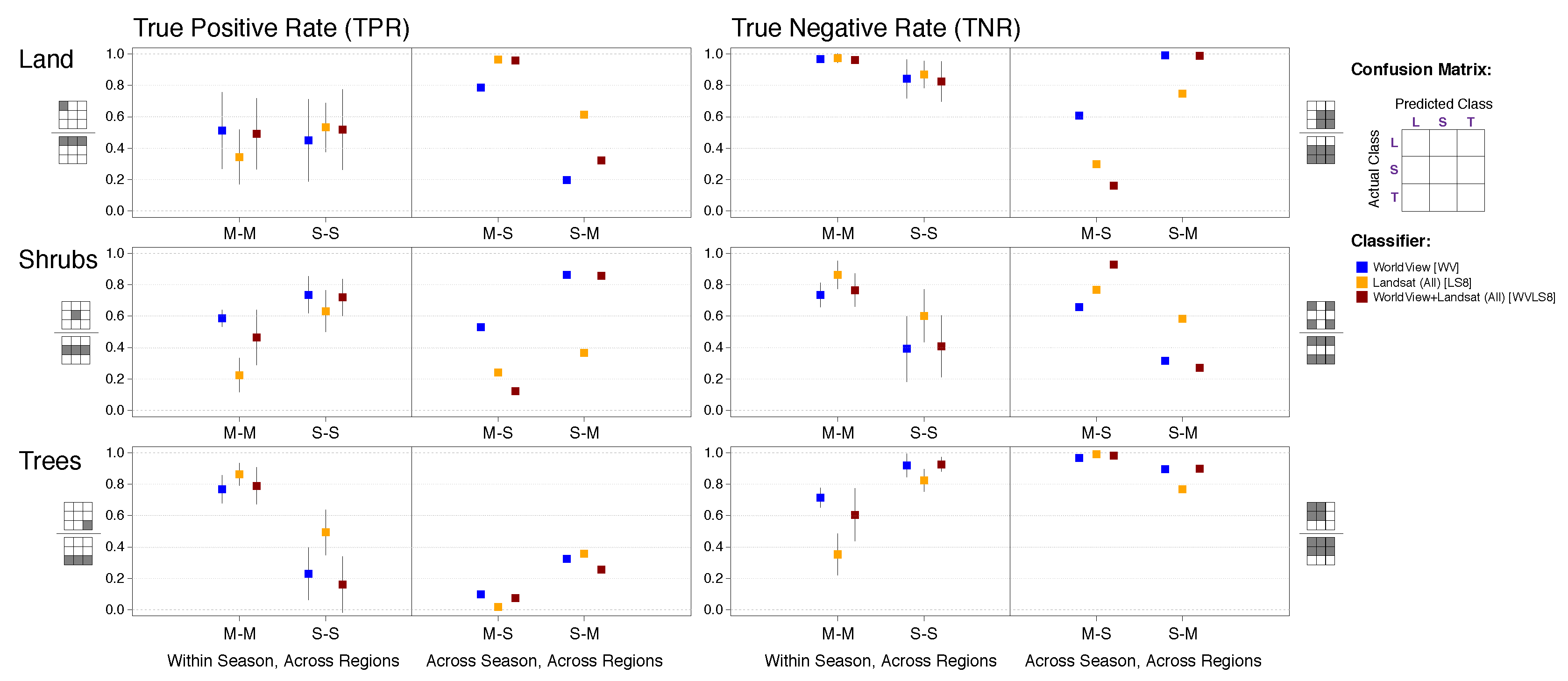
Here, we adopted a k-fold cross validation procedure. We used 5-fold cross-validation in all experiments (i.e., 5 folds, or groups), with random examples allocated to folds stratified by labeled class (i.e., each fold had the same proportion of each class as the full region). We performed classification and accuracy assessment both within and between regions: in “within-region” analysis, we divided the examples in a region into 5 folds. For each experiment, we used all examples in 4 folds for training, and assessed the classification of the examples in the remaining fold. In “between-region” analysis, we used all the examples in 6 or 4 regions (the summer or the winter images). The latter procedure is designed to evaluate the spatial generalization of the classifiers. Thus, we repeat the 5-fold cross validation twice: with all the examples in regions 1–4 (March 2016) and with all the examples in regions 5–10 (September 2015).

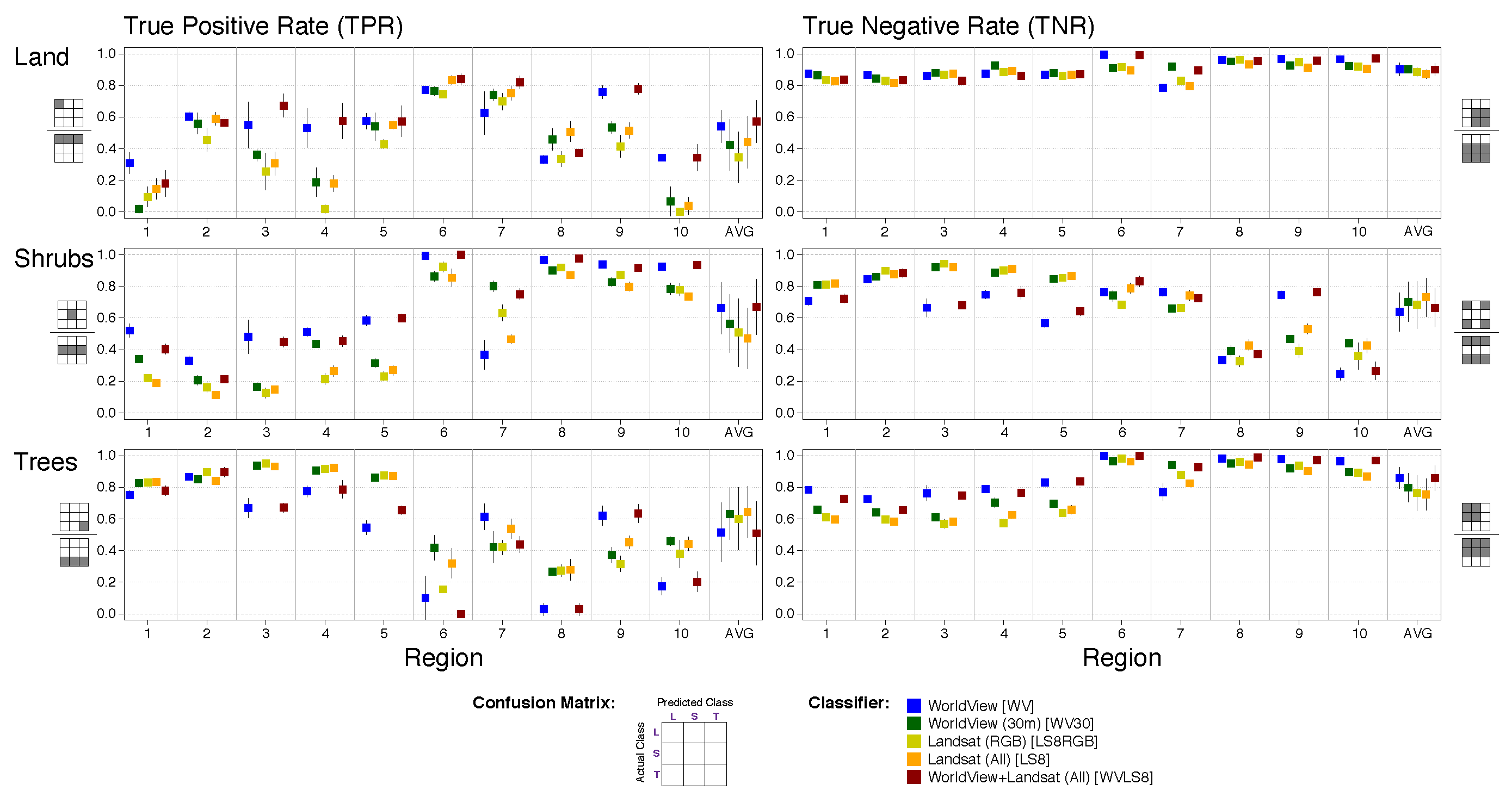
We assess classifier performance using three estimated quantities from 2- and 3- class confusion matrices (e.g., as in [41] for 3-class): (1) True Positive Rate (TPR), or sensitivity, which refers to the percentage of positive examples classified correctly as positive (i.e., positive label = classification as positive); (2) True Negative Rate (TNR), or specificity, which refers to the percentage of negative examples (or “not positive”) that were classified correctly as negative (or as “not positive”) (e.g., if trees are positive and land and shrubs are negative, TNR refers to the percentage of land and shrubs examples that were correctly classified as not trees). Although reporting TPR and TNR is standard practice in a 2-class classification problem, we note that it is especially important to interpret these quantities appropriately when dealing with imbalanced datasets. In our setting, the weight of each class (i.e., the number of per-class examples, Table 1) depends on the coverage of each class in a region.

For each experiment, we calculated mean values and standard errors of TPR and TNR across all 5 folds. When assessing classifier performance by class, standard errors (95% confidence interval) for each metric were calculated across folds based on the number of examples per class per fold.

2.5. Experiment Summary and Ecosystem-Scale Assessments

In summary, we conducted 170 total experiments, with a 5-fold cross-validation: (1) within-region: 5 band/resolution combinations × 10 regions × 3 classifications; and (2) between-region: 5 band/resolution combinations × 4 season combinations. After assessing classifier performance using 5-fold cross-validation (with the exception of cross-season, where we used all the labeled examples from one season to classify the samples in the region sensed in the other season), we used each classifier to do an out-of-sample classification of all pixels in the 1000 km${}^2$ region, and compared total area fractions across classifiers both internally and to existing estimates from the literature.

3. Results

3.1. Within-Region Classifier Performance

Performance metrics (TPR and TNR) of 3-class classification (land, shrubs, trees) by class for each of the 5 spatial/spectral resolution combinations are shown in Figure 3. TNR is higher than the TPR for classification with all inputs, and TNR confidence intervals are on average smaller than those for TPR: this is in large part due to the fact that, as noted above, TNR in a 3-class classification contains confusion between the two negative classes and is thus artificially inflated. The classifiers perform better, in general, when using the high spatial-resolution WorldView Data. Classification with WorldView by itself (WV) and with WorldView + Landsat 8 (WVLS8) (both at 0.3–0.5 m resolution), outperforms classification with Landsat 8 (LS8 and LS8RGB) and with WorldView at a 30 m resolution (WV30); we also observe that classification with WV is not significantly different from classification with WVLS8, indicated by all performance metrics. This suggests that, in this context, the addition of Landsat 8 spectral bands does not add much power to the high spatial-resolution RGB data.

On average, classification with high spatial-resolution inputs outperforms classification with coarser-resolution inputs in differentiating between bare land and shrubs, and is less likely to mis-classify bare land and shrubs as trees. In addition, we find variation in the performance of the classifiers across the study area. In particular regions 6 and 9 stand out for the accurate classification of land and shrubs, as shown in Table 1; this is likely a function of the major predominance of these two classes in those regions (there are simply more examples labeled as trees and shrubs).

The results suggest that classification with WV (high spatial-resolution but only three bands) outperforms classification with the full spectral range of the coarser spatial resolution Landsat (LS8). These results are not enough to tease out the relative importance of Landsat’s non-RGB bands (spectral degrees of freedom) versus WorldView’s pixel size (spatial degrees of freedom). For this reason, we performed an additional experiment designed to conceptually link these two different data sources with two ‘intermediate’ inputs—WV30 (WorldView, aggregated to 30 m pixel size) and LS8RGB (Landsat, using only RGB bands). Conceptually, classification with these two inputs should perform similarly. Indeed, this is the case, although performance is not identical, with WV30 slightly outperforming LS8RGB across the board. We then interpret the differences between classification with WV and WV30 as the impact of decreased spatial resolution with a constant spectral resolution (RGB bands). Similarly, we interpret the differences between classification with LS8RGB and with the full spectral information of Landsat (LS8) as the effect of increased spectral resolution, while spatial resolution is held fixed. Comparing within a given region (e.g., region 9), we see bigger improvement between classification with WV30 and WV than between classification with LS8RGB and LS8. These results indicate that the factor of 100 difference in pixel edge length out-weighs the additional (factor of >10 increase) in spectral degrees of freedom.

Assessment of 2-class classification accuracy with different posterior probability thresholds (Figure 4) suggests that classification with higher-resolution inputs to the classifier (WV and WVLS8) shows more sensitivity to the threshold than classification with lower spatial resolution inputs (LS8RGB, LS8 and WV30). Namely, both TPR and TNR drop more sharply as the posterior probability decreases when classification is performed with WV and WVLS8 than when classification is performed with lower-resolution inputs. This implies that, when classification is performed with high-resolution imagery, it is ‘easier’ for the classifiers to predict an example as positive (i.e., many of the pixels have a high posterior probability value). On the other hand, higher sensitivity to the threshold indicates that the confidence is lower (i.e., if we set the threshold to a low value, we miss positive pixels). An optimal low posterior probability threshold means that it is ‘harder’ for the classifier to predict a positive example than to predict a negative example. A low threshold is appropriate when we don’t want to weight keeping true positive examples more than having excess predicted positive examples (even if the probability they are true is low). Conversely, when the posterior probability threshold is set to a higher value, fewer examples are predicted correctly as positive (we ‘miss’ those with a lower probability value) but also have a much lower false-positive rate.

All of the classifiers perform well in distinguishing land from vegetation (shrubs and trees considered together), though classification with a higher spatial resolution input (WV and WVLS8) shows more sensitivity to the posterior probability threshold. As shown in Figure 4, at a low posterior probability threshold of 0.1, the 2-class classifications of land vs. vegetation and trees vs. shrubs have very high TPR and TNR values, suggesting that the separation of the two types of vegetation is a limiting factor for classifier performance. Indeed, classification of land vs. vegetation is significantly more accurate than classification of trees vs. shrubs, especially when the posterior probability threshold is high. Classification of land vs. vegetation with the higher resolution input (WV and WVLS8) performs worse than classification with the 30 m classifiers (LS8), especially at higher posterior probability thresholds. This is the only analysis we performed where increased spectral information performed better than increased spatial information. However, as discussed below, this is likely an artifact of averaging across regions (and therefore seasons).

The variation in the performance of the classifiers across regions also is meaningful. Performance metrics for images from March (regions 1–4) have less variation both within and across regions than for images from September (regions 5–10), especially for classification with high spatial resolution inputs (WV, WVLS8) and for classification of vegetation (trees, shrubs). March is the rainy season for the region, as vegetation starts to green up; while September is near the beginning of the dry season, where cumulative effects of the previous season’s precipitation should be visible. We would thus naturally expect that classifiers show less variation in performance for differentiating between vegetation classes in March than September, and less overall variation between seasons for classification of land.

3.2. Between-Region Classifier Performance

We next assess the spatial generalization of the classifiers and the extent to which reference data collected from one region can be used to classify other regions. As shown in Figure 5, when using reference points from one region to classify another within the same season, classifiers perform better in March than the average (Figure 3), driven by a larger training data size (number of labeled examples). They perform closer to average or slightly worse in the images sensed in September. The performance difference between the two seasons can again be understood in terms of vegetation differences in monsoonal ecosystems—heterogeneity in rainfall-driven seasonal vegetation would be expected to peak after the rainy season has ended, early in the dry season.

We also run the classification using the labeled examples from March to classify the samples of the region sensed in September and vice versa (shown on the right sides of plots in Figure 5). Performance is worse for classification with all combinations of inputs, and for all classes. While not surprising, these results confirm that seasonality and type of land cover matters when using one region to classify another: the ecosystem changes across seasons, affecting potentially both the reflectance of different classes (discussed below) and the stratification of the training data set (which may not match the test set).

3.3. Seasonality

We did not have access to co-located imagery from different seasons within the same year (the ideal experiment), so we instead chose regions from within the same calendar year, but different seasons, to examine the extent of meaningful variation in the spectral reflectance of the land cover. Though observing seasonal variation is rather intuitive and expected, this analysis is important for explaining differences between and within seasons in classification accuracy. To do this, we examine the reflectance profile of the three investigated land cover types (trees, shrubs, and land) in March (regions 1–4) and in September (regions 5–10). We define the reflectance profile for each type of land cover as the 8-bits average reflectance value of all pixels labeled as a given land cover type, per Landsat 8 and WorldView band. Note that Landsat and WorldView satellites collect data in a different dynamic range. WV2 and WV3 collect data in a dynamic range of 11 and 14 bits, respectively, while Landsat collects data over a 12-bit dynamic range (the data products are delivered in 16-bit unsigned integer format). The down scaling procedure to 8-bit values (which we use for classification) results in different reflectance values between the satellites. As expected, results show seasonal variations in the spectral profile of the three land cover types, which is observed in both Landsat 8 and WorldView (Figure 6,

Table A3. Statistics for Landsat 8 reflectance values of training data set, per class and season (p-values shown for 95% confidence interval).

	Band:	B1	B2	B3	B4	B5	B6	B7	B8	B10	B11
LAND		Regions 1–4 (March) (n = 235)
	Mean	35.30	31.37	30.86	31.37	77.09	73.19	45.96	30.47	193.95	190.82
	Std. Err.	0.38	0.42	0.46	0.60	0.84	1.05	0.83	0.49	0.14	0.12
		Regions 5–10 (September) (n = 1150)
	Mean	35.19	32.30	34.35	44.86	68.62	103.52	76.75	37.76	212.79	210.55
	Std. Err.	0.11	0.14	0.20	0.27	0.33	0.47	0.44	0.22	0.12	0.11
		t-tests of equal means (March/September)
	(t-stat)	−0.30	2.11	6.88	20.43	−9.38	26.38	32.79	13.54	104.22	117.89
	(p-value)	0.77	0.036	0.000	0.000	0.000	0.000	0.000	0.000	0.000	0.000
TREES		Regions 1–4 (March) (n = 2852)
	Mean	33.72	28.99	25.79	22.79	68.32	56.28	31.71	24.32	193.13	190.12
	Std. Err.	0.12	0.13	0.14	0.16	0.20	0.21	0.17	0.14	0.03	0.03
		Regions 5–10 (September) (n = 1759)
	Mean	33.98	30.09	27.46	31.48	53.82	76.92	51.76	28.60	208.05	206.34
	Std. Err.	0.05	0.07	0.10	0.15	0.30	0.31	0.27	0.11	0.08	0.07
		t-tests of equal means (March/September)
	(t-stat)	1.97	7.55	10.01	39.89	−40.38	55.23	63.43	23.32	181.03	204.88
	(p-value)	0.048	0.000	0.000	0.000	0.000	0.000	0.000	0.000	0.000	0.000
SHRUBS		Regions 1–4 (March) (n = 906)
	Mean	35.28	30.93	28.62	26.66	72.28	62.80	37.34	27.49	193.27	190.24
	Std. Err.	0.28	0.31	0.32	0.36	0.44	0.45	0.37	0.33	0.07	0.06
		Regions 5–10 (September) (n = 3073)
	Mean	34.09	30.35	28.47	33.59	53.42	82.77	57.29	30.04	208.43	206.37
	Std. Err.	0.04	0.05	0.08	0.12	0.18	0.24	0.21	0.09	0.06	0.06
		t-tests of equal means (March/September)
	(t-stat)	1.97	−1.87	−0.47	18.41	−39.64	39.62	47.12	7.44	166.37	185.38
	(p-value)	0.048	0.062	0.635	0.000	0.000	0.000	0.000	0.002	0.000	0.000

and

Table A4. Statistics for WorldView reflectance values of training data set, per class and season (p-values shown for 95% confidence interval).

	Band:	B1	B2	B3
LAND	Regions 1–4 (March) (n = 373)
	Mean	144.27	135.65	132.74
	Std. Err.	1.60	1.64	1.66
	Regions 5–10 (September) (n = 1763)
	Mean	178.32	148.44	123.47
	Std. Err.	0.95	1.00	0.94
	t-tests of equal means (Mar/Sept)
	(t-stat)	18.33	6.67	−4.88
	(p-value)	0.000	0.000	0.000
TREES	Regions 1–4 (March) (n = 2021)
	Mean	82.97	84.02	88.94
	Std. Err.	0.40	0.38	0.37
	Regions 5–10 (September) (n = 769)
	Mean	110.81	100.90	93.67
	Std. Err.	1.05	0.84	0.83
	t-tests of equal means (Mar/Sept)
	(t-stat)	24.82	18.23	5.20
	(p-value)	0.000	0.000	0.000
SHRUBS	Regions 1–4 (March) (n = 1599)
	Mean	102.83	100.61	102.40
	Std. Err.	0.58	0.56	0.54
	Regions 5–10 (September) (n = 3450)
	Mean	134.67	121.42	110.11
	Std. Err.	0.58	0.54	0.45
	t-tests of equal means (Mar/Sept)
	(t-stat)	38.96	26.88	10.98
	(p-value)	0.000	0.000	0.000

). In September (the dry season), the reflectance of land and trees is significantly ($p<0.05$) higher than in March (the rainy season) in all Landsat bands, besides the near-infrared wavelength (B5). Shrubs, however, are characterized by a relatively similar reflectance in Landsat’s blue and green bands (B2 and B3, respectively) in March and in September, but a seasonal difference in the red band (drier or ‘browner’ vegetation in September).

Consistent with the high reflectance of live vegetation in the near infrared wavelength, the reflectance of the three land cover types is significantly ($p=0.000$) higher in the near infrared wavelength (B5) in March than in September. Seasonal variation in the reflectance of trees and shrubs is also observed in WorldView imagery. In September, the reflectance of trees and shrubs are significantly ($p=0.000$) higher than in March, in all bands. Moreover, the results show variations in the reflectance of the land cover also within season. As illustrated in Figure 6 (the reflectance profile of the land cover in Landsat and WorldView), the reflectance of shrubs is higher than the reflectance of trees in all Landsat and WorldView bands, in March and in September. However, the difference between the reflectance of trees and shrubs is more significant in March than in September. The difference between the mean reflectance of trees and shrubs is significantly ($p<0.01$) larger in March than in September in all bands besides Landsat’s thermal bands (bands B10 and B11) (

Table A5. Two-sample t-test with unequal variances: comparison of mean reflectance (Landsat 8 and WorldView) of trees and shrubs.

	Landsat
	B2			B3			B4
	Diff.	Std. Err.	Pr($\left|T\right|>\left|t\right|$)	Diff.	Std. Err.	Pr($\left|T\right|>\left|t\right|$)	Diff.	Std. Err.	Pr($\left|T\right|>\left|t\right|$)
March	−1.941	0.335	0.000	−2.832	0.345	0.000	−3.871	0.389	0.000
September	−0.256	0.080	0.001	−1.004	0.122	0.000	−2.110	0.195	0.000
	B5			B6			B7
	Diff.	Std. Err.	Pr($\left|T\right|>\left|t\right|$)	Diff.	Std. Err.	Pr($\left|T\right|>\left|t\right|$)	Diff.	Std. Err.	Pr($\left|T\right|>\left|t\right|$)
March	−3.956	0.484	0.000	−6.515	0.491	0.000	−5.636	0.407	0.000
September	0.398	0.347	0.252	−5.849	0.391	0.000	−5.537	0.337	0.000
	B8			B9			B10
	Diff.	Std. Err.	Pr($\left|T\right|>\left|t\right|$)	Diff.	Std. Err.	Pr($\left|T\right|>\left|t\right|$)	Diff.	Std. Err.	Pr($\left|T\right|>\left|t\right|$)
March	−3.166	0.361	0.000	−0.143	0.075	0.058	−0.120	0.070	0.088
September	−1.443	0.146	0.000	−0.384	0.097	0.000	−0.031	0.094	0.743
	WorldView
	B1			B2			B3
	Diff.	Std. Err.	Pr($\left|T\right|>\left|t\right|$)	Diff.	Std. Err.	Pr($\left|T\right|>\left|t\right|$)	Diff.	Std. Err.	Pr($\left|T\right|>\left|t\right|$)
March	−19.86	0.704	0.000	−16.59	0.676	0.000	−13.46	0.651	0.000
September	−23.86	1.197	0.000	−20.51	1.001	0.000	−16.45	0.946	0.000

). In other words, the difference between the reflectance of trees and shrubs is significantly larger in the rainy (or “greener”) season than in the dry season.

The variations in the reflectance of the land cover (within and between seasons) is also expressed by the examined L8-based spectral indices (

Table A6. Statistics for NDVI, EVI, NDWI, NDBI and UI spectral indices (calculated with Landsat 8), per season, with comparison for trees and shrubs.

		NDVI		EVI		NDWI		NDBI		UI
		March	Sep.	March	Sep.	March	Sep.	March	Sep.	March	Sep.
Land	Mean	0.425	0.212	4.770	1.014	−0.427	−0.334	−0.032	0.202	−0.262	0.0052
	Std. Err.	0.005	0.002	2.280	0.124	0.004	0.002	0.005	0.003	0.007	0.003
Trees	Mean	0.504	0.257	−5.930	0.861	−0.453	−0.316	−0.099	0.179	−0.372	−0.017
	Std. Err.	0.002	0.002	0.681	0.374	0.001	0.002	0.001	0.003	0.002	0.003
Shrubs	Mean	0.468	0.228	−1.053	0.941	−0.435	−0.301	−0.073	0.217	−0.326	0.033
	Std. Err.	0.003	0.000	1.721	0.212	0.003	0.000	0.002	0.002	0.003	0.002
		t-tests of equal means (unequal variances) for trees and shrubs (within season)
t-test *	(t-stat)	10.431	12.855	−2.630	−0.190	−6.210	−8.680	−9.940	−13.032	−13.273	−15.369
	(p-value)	0.000	0.000	0.010	0.850	0.000	0.000	0.000	0.000	0.000	0.000

). Trees and shrubs are characterized by significantly ($p<0.05$) different NDVI, NDWI, NDBI and UI values, both in the dry and in the rainy seasons. In both seasons, the NDVI value of trees in significantly ($p=0.000$) higher than the NDVI value of shrubs. Moreover, the average NDVI value of the three land cover types is significantly higher in March than in September (Figure 7 presents the distribution of NDVI and NDWI values for trees and shrubs pixels, in March and in September). Similarly, the average NDWI of trees is significantly lower than of shrubs, and significantly lower in March than in September ($p=0.000$, for both). This result is consistent with the higher reflection of live vegetation in the near infrared wavelength than in the green wavelength, especially in the rainy season. On the other hand, the average NDBI and UI values of all land cover types are significantly ($p=0.000$) higher in September than in March (higher values of these indices indicate presence of bare land and soil, and less vegetation).

Taken together, the variations in spectral reflectance—even in the visible RGB bands—indicate that the cross-season performance differences and the poor performance of training sets on imagery from the opposite season (Figure 5) are likely to be driven by actual changes in the reflectance of different land cover types between wet and dry seasons. This has important implications for ecosystem-scale assessments based on satellite imagery.

3.4. Full Area Estimates

To test the application potential of high-resolution classifiers over large areas, we used the labeled examples from each of the ten regions as training sets to then classify each region (using three classes), a total area of 1000 km${}^2$. Figure 8 shows two representative samples of the classification in subsets of two of the ten regions. When classification is performed with high spatial resolution input, the distinction between features in the heterogeneous semi-arid landscape is clear, and contrasts profoundly with the coarse (by comparison) Landsat-based classifier.

Table A8. Full area estimates. Percentage of each region covered by each class, by classifier. Note: for full classification of each 1000 km${}^2$ region, we used the labeled examples from within that region as a training set. (Percentages may not add perfectly to 100 due to rounding.)

		1	2	3	4	5	6	7	8	9	10	Average
WV	L	4.2	14.5	7.4	7.0	15.9	53.8	37.8	21.1	33.7	6.7	20.2
	S	44.6	20.2	49.9	42.1	52.6	45.9	48.7	76.8	60.2	88.2	52.9
	T	51.1	65.3	42.7	51.0	31.5	0.3	13.5	2.1	6.1	5.1	26.9
LS8	L	2.3	12.5	2.6	4.5	10.8	49.8	37.5	11.7	10.8	2.6	14.5
	S	25.1	13.7	10.7	15.6	16.2	43.3	32.7	78.6	71.6	75.7	38.3
	T	72.6	73.8	86.7	79.9	73.0	6.9	29.7	9.7	17.7	21.7	47.2
WVLS8	L	3.6	14.5	7.8	8.0	15.2	55.4	40.0	28.2	35.0	6.3	21.4
	S	40.1	15.8	46.4	39.0	47.3	44.4	47.9	70.6	58.9	90.1	50.1
	T	56.4	69.7	45.8	53.0	37.5	0.3	12.1	1.2	6.2	3.7	28.6

shows the percentage of each 100 km${}^2$ region covered by each land cover class. The totals derived from the WV and LS8 classifiers vary widely, with the greatest differences between trees and shrubs. This further supports what the 2-class performance metrics (Figure 4) suggested: namely that classification with high spatial resolution data outperforms in distinguishing between these two vegetation types.

The WV classification estimates that 20% of the area is bare land, while 27% is tree/tree canopy and 53% is seasonal vegetation (shrubs); this is very close, as would be expected, to the distribution of our reference data in the original random selection of points. The full area estimates for classification with LS8 (15%/38%/47% for land, shrubs, and trees, respectively) is also closely aligned with the reference data that was labeled according to the buffer approach. However, Figure 2 and Figure 8 show the fundamental issue with classification based on a coarse spatial resolution input: because the spatial scale is much larger than the scale of variation in land cover, the classification overestimates land cover for each class in some areas, and underestimates it in others. While the overall totals or averages may not differ dramatically from the finer-scale classifier, performance is clearly worse. In particular, bare land and seasonal vegetation often exist in narrow or winding tracks and sparse patterns, not within full pixels, in the Sertão, so it is fundamentally underestimated when classification is performed with coarser-resolution inputs; even a small fraction of trees within one 30 m resolution pixel may affect the spectral characteristics of the pixel, and lead to over-classification of trees. This problem of ‘mixed-class pixels’—when two or more distinct classes may fall within a single pixel—has been widely addressed in the literature. The extent to which this occurs is dependent on the spatial resolution of the sensor and the spatial variability of the observed surface [42]. In this example of different types of vegetation, the mixed pixel problem appears to play a dominant role in the accuracy of the classification.

Lastly, we compare our full-area estimates to the estimates of a recent global dryland forest assessment by Bastin et al. [10], who use similar high-resolution imagery but a sampling and manual image interpretation approach to estimate tree canopy cover across the world’s drylands (that is, they sample regions, sub-sample pixels within those regions, and manually label them; they do not run any classification of the full area). We use their data and match local estimates to our full-region estimates as shown in Figure 9. Our classification with high spatial resolution inputs (WV and WVLS8) estimate a higher percentage of tree cover than Bastin et al. (WV: Mean 26.9%, Standard Deviation (Std.) 24.3%; Bastin: Mean 20.5%, Std. 34.0%), with the spatially-coarser classifier (LS8) overestimating treecover (LS8: Mean 47.2%, Std. 32.5%), largely due to the ‘mixed pixel’ problem described above and illustrated in Figure 8 and Table A8.

4. Discussion

Here, we show that pixel-based image classification with high spatial resolution satellite imagery and with only three bands—RGB (WV)—outperforms classification using inputs with a higher spectral but lower spatial resolution satellite imagery (LS8) for classification of non-built-up landcover in the semi-arid landscapes of the Brazilian Sertão. Our results are to some extent intuitive in that they show that high spatial resolution input gives us much more detailed information on land-cover patterns than medium or coarse spatial resolution input (even with higher spectral resolution). This study complements an emerging literature on why spatial resolution is considered one of the most significant emerging factors for accurate complex urban land cover mapping (e.g., [43]) and is especially essential when mapping heterogeneous and fragmented landscapes [44] as found in the semi-arid Brazilian Sertão.

We demonstrate that high spatial resolution imagery helps to mitigate the problem identified in previous literature as ‘mixed class’ pixels (e.g., [45]). In particular, we show that classification with high spatial resolution data as input to the classifier improves the ability to distinguish between more permanent and seasonal features in the landscape (trees versus shrubs). The distinction between trees and shrubs is critical for ecosystem assessment in dryland regions because while tree cover in semi-arid regions is an important driver of overall landscape processes and carbon sequestration, seasonal variation in shrub and grass cover is a principal driver of the interannual variability in the carbon cycle [5,46]. Our results thus complement recent studies showing that using high spatial resolution imagery can increase the accuracy of above-ground biomass estimation [47,48].

Although we highlight here that increased spatial resolution improves classifier performance, we do not discount the importance of spectral information, and, in fact, show that, even in the visible bands, spectral differences across seasons are meaningful in semi-arid regions. Although this study was limited by the WorldView imagery made available to us, use of the full spectral information available from WorldView (i.e., high spatial and high spectral resolution) would be extremely valuable for this type of assessment.

Our results confirm that seasonality and type of land cover matters when using one region to classify another: the ecosystem changes across seasons, affecting potentially both the spectral reflectance of different classes and the stratification of the reference training data set (which may not match the test set). However, we find that the seasonal difference in all three classes (trees, shrubs, and land) does not seem to be bigger in the RGB bands compared to other bands (at least according to the t-stat measures), implying that the high spatial-resolution RGB data is sufficient for detection of seasonal differences in the distribution of vegetation. We nevertheless emphasize that larger-scale implementations of this kind of classification for ecosystem assessments need to be undertaken with seasonality in mind. This is not new information for those already familiar with or working in semi-arid regions, but it is a distinct departure from the way treecover assessments are done in more dense forests.

Many previous studies utilize publicly available data for land cover mapping, including Landsat and Sentinel (although Sentinel-2 now offers spectral data at 10 m resolution, this pixel size is still too large to allow identification of many of the features that exists in semi-arid landscapes). Here, we compare classification with Landsat-8 (LS8) and with high-resolution data (WV) and demonstrate why, as described in [49], higher-resolution data is preferable to lower-resolution data when a landscape has small features and/or fine-scale variation in LULC, when a large portion of LULC change patches are smaller than the pixel size at lower-resolutions, and when high accuracy is necessary to inform decisions.

Our full area estimates of treecover in the Sertão are higher than, but not profoundly different from, the most recent attempt to quantify treecover in the world’s drylands [10]. That effort used a sampling and image interpretation approach (but not classification) in an effort to deal both with ‘mixed pixel’ problems and seasonality issues. Both Bastin et al.’s approach and ours here require a human-in-the loop to either label examples (this study) or to do the classification itself (Bastin et al.). One benefit of our approach is that it is scalable to classify large-scale regions, as opposed to providing a sample-based estimate of the total quantity of interest. We have also shown that, within season, reference data can be used successfully across larger swaths with no reduction in performance. Finally, we classify the three main landcover types (bare land, trees, seasonal vegetation), as opposed to simply one.

These three features of supervised pixel-based image classification approach would be especially important for applications like monitoring land degradation at finer spatial scales (e.g., farm level seasonal changes) or estimating compliance with (for example) Brazil’s Forest Code, which stipulates that 20% of all private landholdings outside the Amazon be preserved in native habitat [50], comprised of a wide range of vegetation types. Existing Landsat-based forest cover data sets (e.g., [8]) are able to assess changes in dense forest cover in the Amazon (where the Forest Code preservation requirement is 80%), but here we show that basic supervised image classification using high-resolution imagery in Google Earth Engine could be used to fully assess the state of compliance in the Sertão.

We acknowledge that at present very real financial obstacles exist to using private high-resolution data like that from WorldView for assessments of large-scale regions. However, as more and more high-resolution remotely sensed data become available to the research community, our study provides the best existing example of how they could be leveraged, in conjunction with the processing power of platforms like GEE, to conduct novel, and critical, large-scale ecosystem assessments of the world’s semi-arid regions. Furthermore, in this study, we relied on WorldView orthorectified pan-sharpened 3-band imagery (using off the shelf imagery as delivered by DigitalGlobe). Extension to our work should utilize WorldView multispectral imagery to fully understand the contribution of the spatial and spectral dimension of the input data. In addition, understanding temporal dynamics in land cover patterns, including changes in vegetation land cover, requires radiometrically calibrated spectral data that was not available to us in this study.

5. Conclusions

This study shows that WorldView RGB imagery in a spatial resolution of 0.3–0.5 m can be utilized for high-quality and accurate classification of three types of natural landcover in the semi-arid Brazilian Sertão (land, trees and shrubs), outperforming classification with 30 m multi-spectral Landsat-8 imagery as input. We show that this superior performance classifying bare land, trees, and shrubs (here all non-tree vegetation) stems from two features of the high spatial resolution imagery. First, WorldView imagery, even with fewer spectral bands (RGB), allows for identifying small objects, such as individual trees and shrubs, that are captured in Landsat imagery as part of ‘mixed-class’ pixels; i.e., features smaller than the spatial resolution of the spectral Landsat imagery. Second, even with only the visible bands (RGB), classification with WorldView imagery as input can help to distinguish between trees and other seasonal vegetation with higher accuracy than with Landsat. This holds across the rainy and the dry seasons, although we show that, for the Sertão (and likely other semi-arid regions), performance is poor across seasons—a critical note for researchers using pixel-based classification in these agro-ecological zones.

By combining high spatial resolution imagery with the computation power of Google Earth Engine, and prototyping our classification on a 1000 km${}^2$ area, we demonstrate the first viable methodology for conducting large-scale, high-resolution, and repeated ecosystem assessments of the world’s semi-arid regions. Our full-area estimates of treecover differ from estimates based on both Landsat (which overestimate trees) and high-resolution sub-sampling and image-interpretation approaches, which appear to underestimate treecover, perhaps due to sparse sampling in heterogeneous areas. This implies that WorldView imagery, combined with relatively simple methods for supervised image classification in Google Earth Engine, can be utilized for totally new and perhaps counterintuitive land cover statistics of global semi-arid regions and the world’s drylands.

Semi-arid regions, as home to hundreds of millions of smallholder farmers, are hotspots for food security and climate adaptation. Additionally, both longer-run trends in ecosystem degradation and land use changes, as well as interannual variability in seasonal vegetation, are key drivers of the global carbon cycle. Seasonal, global, and high-resolution assessments of the world’s semi-arid regions based on the methodology described here would thus constitute a tremendously valuable new data source to understand earth system dynamics from scales small—e.g., the drivers of land use change at the farm scale—to large—e.g., land-atmosphere coupling globally.

References

1. Reynolds, J.F.; Smith, D.M.S.; Lambin, E.F.; Turner, B.; Mortimore, M.; Batterbury, S.P.; Downing, T.E.; Dowlatabadi, H.; Fernández, R.J.; Herrick, J.E.; et al. Global desertification: Building a science for dryland development. Science 2007, 316, 847–851. [Google Scholar] [CrossRef] [PubMed]
2. Koster, R.D.; Dirmeyer, P.A.; Guo, Z.; Bonan, G.; Chan, E.; Cox, P.; Gordon, C.; Kanae, S.; Kowalczyk, E.; Lawrence, D.; et al. Regions of strong coupling between soil moisture and precipitation. Science 2004, 305, 1138–1140. [Google Scholar] [CrossRef] [PubMed]
3. Oyama, M.D.; Nobre, C.A. Climatic consequences of a large-scale desertification in northeast Brazil: A GCM simulation study. J. Clim. 2004, 17, 3203–3213. [Google Scholar] [CrossRef]
4. Seddon, A.; Macias-Fauria, M.; Long, P.; Benz, D.; Willis, K. Sensitivity of global terrestrial ecosystems to climate variability. Nature 2016, 531, 229–232. [Google Scholar] [CrossRef] [PubMed]
5. Poulter, B.; Frank, D.; Ciais, P.; Myneni, R.B.; Andela, N.; Bi, J.; Broquet, G.; Canadell, J.G.; Chevallier, F.; Liu, Y.Y.; et al. Contribution of semi-arid ecosystems to interannual variability of the global carbon cycle. Nature 2014, 509, 600–603. [Google Scholar] [CrossRef] [PubMed]
6. Oyama, M.D.; Nobre, C.A. A new climate-vegetation equilibrium state for tropical South America. Geophys. Res. Lett. 2003, 30. [Google Scholar] [CrossRef]
7. Huang, J.; Yu, H.; Guan, X.; Wang, G.; Guo, R. Accelerated dryland expansion under climate change. Nat. Clim. Chang. 2016, 6, 166–171. [Google Scholar] [CrossRef]
8. Hansen, M.C.; Potapov, P.V.; Moore, R.; Hancher, M.; Turubanova, S.A.; Tyukavina, A.; Thau, D.; Stehman, S.V.; Goetz, S.J.; Loveland, T.R.; et al. High-resolution global maps of 21st-century forest cover change. Science 2013, 342, 850–853. [Google Scholar] [CrossRef] [PubMed]
9. Fensholt, R.; Langanke, T.; Rasmussen, K.; Reenberg, A.; Prince, S.D.; Tucker, C.; Scholes, R.J.; Le, Q.B.; Bondeau, A.; Eastman, R.; et al. Greenness in semi-arid areas across the globe 1981–2007—An Earth Observing Satellite based analysis of trends and drivers. Remote Sens. Environ. 2012, 121, 144–158. [Google Scholar] [CrossRef]
10. Bastin, J.F.; Berrahmouni, N.; Grainger, A.; Maniatis, D.; Mollicone, D.; Moore, R.; Patriarca, C.; Picard, N.; Sparrow, B.; Abraham, E.M.; et al. The extent of forest in dryland biomes. Science 2017, 356, 635–638. [Google Scholar] [CrossRef] [PubMed]
11. Barsi, J.A.; Lee, K.; Kvaran, G.; Markham, B.L.; Pedelty, J.A. The spectral response of the Landsat-8 operational land imager. Remote Sens. 2014, 6, 10232–10251. [Google Scholar] [CrossRef]
12. Gorelick, N.; Hancher, M.; Dixon, M.; Ilyushchenko, S.; Thau, D.; Moore, R. Google Earth Engine: Planetary-scale geospatial analysis for everyone. Remote Sens. Environ. 2017, 202, 18–27. [Google Scholar] [CrossRef]
13. Patel, N.N.; Angiuli, E.; Gamba, P.; Gaughan, A.; Lisini, G.; Stevens, F.R.; Tatem, A.J.; Trianni, G. Multitemporal settlement and population mapping from Landsat using Google Earth Engine. Int. J. Appl. Earth Obs. Geoinf. 2015, 35 Pt B, 199–208. [Google Scholar] [CrossRef]
14. Trianni, G.; Lisini, G.; Angiuli, E.; Moreno, E.A.; Dondi, P.; Gaggia, A.; Gamba, P. Scaling up to national/regional urban extent mapping using Landsat data. IEEE J. Sel. Top. Appl. Earth Obs. Remote Sens. 2015, 8, 3710–3719. [Google Scholar] [CrossRef]
15. Goldblatt, R.; You, W.; Hanson, G.; Khandelwal, A.K. Detecting the boundaries of urban areas in India: A dataset for pixel-based image classification in Google Earth Engine. Remote Sens. 2016, 8, 634. [Google Scholar] [CrossRef]
16. Liang, S.; Fang, H.; Chen, M. Atmospheric correction of Landsat ETM+ land surface imagery. I. Methods. IEEE Trans. Geosci. Remote Sens. 2001, 39, 2490–2498. [Google Scholar] [CrossRef]
17. Li, H.; Wang, C.; Zhong, C.; Su, A.; Xiong, C.; Wang, J.; Liu, J. Mapping urban bare land automatically from Landsat imagery with a simple index. Remote Sens. 2017, 9, 249. [Google Scholar] [CrossRef]
18. He, C.; Shi, P.; Xie, D.; Zhao, Y. Improving the normalized difference built-up index to map urban built-up areas using a semiautomatic segmentation approach. Remote Sens. Lett. 2010, 1, 213–221. [Google Scholar] [CrossRef]
19. Gislason, P.O.; Benediktsson, J.A.; Sveinsson, J.R. Random Forests for land cover classification. Pattern Recognit. Lett. 2006, 27, 294–300. [Google Scholar] [CrossRef]
20. Rodriguez-Galiano, V.F.; Ghimire, B.; Rogan, J.; Chica-Olmo, M.; Rigol-Sanchez, J.P. An assessment of the effectiveness of a random forest classifier for land-cover classification. ISPRS J. Photogramm. Remote Sens. 2012, 67, 93–104. [Google Scholar] [CrossRef]
21. Jean, N.; Burke, M.; Xie, M.; Davis, W.M.; Lobell, D.B.; Ermon, S. Combining satellite imagery and machine learning to predict poverty. Science 2016, 353, 790–794. [Google Scholar] [CrossRef] [PubMed]
22. Stevens, F.R.; Gaughan, A.E.; Linard, C.; Tatem, A.J. Disaggregating Census Data for Population Mapping Using Random Forests with remotely-sensed and ancillary data. PLoS ONE 2015, 10, e0107042. [Google Scholar] [CrossRef] [PubMed]
23. Guan, H.; Li, J.; Chapman, M.; Deng, F.; Ji, Z.; Yang, X. Integration of orthoimagery and lidar data for object-based urban thematic mapping using random forests. Int. J. Remote Sens. 2013, 34, 5166–5186. [Google Scholar] [CrossRef]
24. Zhang, H.; Zhang, Y.; Lin, H. Urban land cover mapping using random forest combined with optical and SAR data. In Proceedings of the 2012 IEEE International Geoscience and Remote Sensing Symposium, Munich, Germany, 22–27 July 2012; pp. 6809–6812. [Google Scholar]
25. Du, P.; Samat, A.; Waske, B.; Liu, S.; Li, Z. Random forest and rotation forest for fully polarized SAR image classification using polarimetric and spatial features. ISPRS J. Photogramm. Remote Sens. 2015, 105, 38–53. [Google Scholar] [CrossRef]
26. Aguirre-Gutiérrez, J.; Seijmonsbergen, A.C.; Duivenvoorden, J.F. Optimizing land cover classification accuracy for change detection, a combined pixel-based and object-based approach in a mountainous area in Mexico. Appl. Geogr. 2012, 34, 29–37. [Google Scholar] [CrossRef]
27. Whiteside, T.; Ahmad, W. A comparison of object-oriented and pixel-based classification methods for mapping land cover in northern Australia. In Proceedings of the SSC2005 Spatial Intelligence, Innovation and Praxis: The National Biennial Conference of the Spatial Sciences Institute, September 2005; Spatial Sciences Institute: Melbourne, Australia, 2005; pp. 1225–1231. [Google Scholar]
28. Myint, S.W.; Gober, P.; Brazel, A.; Grossman-Clarke, S.; Weng, Q. Per-pixel vs. object-based classification of urban land cover extraction using high spatial resolution imagery. Remote Sens. Environ. 2011, 115, 1145–1161. [Google Scholar] [CrossRef]
29. Whiteside, T.G.; Boggs, G.S.; Maier, S.W. Comparing object-based and pixel-based classifications for mapping savannas. Int. J. Appl. Earth Obs. Geoinf. 2011, 13, 884–893. [Google Scholar] [CrossRef]
30. Bhaskaran, S.; Paramananda, S.; Ramnarayan, M. Per-pixel and object-oriented classification methods for mapping urban features using Ikonos satellite data. Appl. Geogr. 2010, 30, 650–665. [Google Scholar] [CrossRef]
31. Duro, D.C.; Franklin, S.E.; Dubé, M.G. A comparison of pixel-based and object-based image analysis with selected machine learning algorithms for the classification of agricultural landscapes using SPOT-5 HRG imagery. Remote Sens. Environ. 2012, 118, 259–272. [Google Scholar] [CrossRef]
32. Dingle Robertson, L.; King, D.J. Comparison of pixel-and object-based classification in land cover change mapping. Int. J. Remote Sens. 2011, 32, 1505–1529. [Google Scholar] [CrossRef]
33. Wu, T.F.; Lin, C.J.; Weng, R.C. Probability estimates for multi-class classification by pairwise coupling. J. Mach. Learn. Res. 2004, 5, 975–1005. [Google Scholar]
34. Zadrozny, B.; Elkan, C. Transforming classifier scores into accurate multiclass probability estimates. In Proceedings of the Eighth ACM SIGKDD International Conference on Knowledge Discovery and Data Mining, Edmonton, AB, Canada, 23–26 July 2002; pp. 694–699. [Google Scholar]
35. Pal, M. Random forest classifier for remote sensing classification. Int. J. Remote Sens. 2005, 26, 217–222. [Google Scholar] [CrossRef]
36. Kulkarni, V.Y.; Sinha, P.K. Random forest classifiers: A survey and future research directions. Int. J. Adv. Comput. 2013, 36, 1144–1153. [Google Scholar]
37. Kohavi, R. A study of cross-validation and bootstrap for accuracy estimation and model selection. In Proceedings of the 14th International Joint Conference on Artificial Intelligence, Montreal, QC, Canada, 20–25 August 1995; pp. 1137–1143. [Google Scholar]
38. Rodriguez, J.D.; Perez, A.; Lozano, J.A. Sensitivity analysis of k-Fold cross validation in prediction error estimation. IEEE Trans. Pattern Anal. Mach. Intell. 2010, 32, 569–575. [Google Scholar] [CrossRef] [PubMed]
39. Salzberg, S.L. On comparing classifiers: Pitfalls to avoid and a recommended approach. Data Min. Knowl. Discov. 1997, 1, 317–328. [Google Scholar] [CrossRef]
40. Arlot, S.; Celisse, A. A survey of cross-validation procedures for model selection. Stat. Surv. 2010, 4, 40–79. [Google Scholar] [CrossRef]
41. Beleites, C.; Salzer, R.; Sergo, V. Validation of soft classification models using partial class memberships: An extended concept of sensitivity & co. applied to grading of astrocytoma tissues. Chemom. Intell. Lab. Syst. 2013, 122, 12–22. [Google Scholar]
42. Barnsley, M. Digital remotely-sensed data and their characteristics. Geogr. Inf. Syst. 1999, 1, 451–466. [Google Scholar]
43. Momeni, R.; Aplin, P.; Boyd, D.S. Mapping complex urban land cover from spaceborne imagery: The influence of spatial resolution, spectral band set and classification approach. Remote Sens. 2016, 8, 88. [Google Scholar] [CrossRef]
44. Chen, D.; Stow, D.; Gong, P. Examining the effect of spatial resolution and texture window size on classification accuracy: An urban environment case. Int. J. Remote Sens. 2004, 25, 2177–2192. [Google Scholar] [CrossRef]
45. Suwanprasit, C.; Srichai, N. Impacts of spatial resolution on land cover classification. Proc. Asia-Pac. Adv. Netw. 2012, 33, 39–47. [Google Scholar] [CrossRef]
46. Ahlström, A.; Raupach, M.R.; Schurgers, G.; Smith, B.; Arneth, A.; Jung, M.; Reichstein, M.; Canadell, J.G.; Friedlingstein, P.; Jain, A.K.; et al. The dominant role of semi-arid ecosystems in the trend and variability of the land CO2 sink. Science 2015, 348, 895–899. [Google Scholar] [CrossRef] [PubMed]
47. Lu, D.; Hetrick, S.; Moran, E. Land cover classification in a complex urban-rural landscape with QuickBird imagery. Photogramm. Eng. Remote Sens. 2010, 76, 1159–1168. [Google Scholar] [CrossRef]
48. Meng, B.; Ge, J.; Liang, T.; Yang, S.; Gao, J.; Feng, Q.; Cui, X.; Huang, X.; Xie, H. Evaluation of remote sensing inversion error for the Above-Ground Biomass of Alpine Meadow Grassland based on multi-source satellite data. Remote Sens. 2017, 9, 372. [Google Scholar] [CrossRef]
49. Fisher, J.R.; Acosta, E.A.; Dennedy-Frank, P.J.; Kroeger, T.; Boucher, T.M. Impact of satellite imagery spatial resolution on land use classification accuracy and modeled water quality. Remote Sens. Ecol. Conserv. 2017. [Google Scholar] [CrossRef]
50. Soares-Filho, B.; Rajão, R.; Macedo, M.; Carneiro, A.; Costa, W.; Coe, M.; Rodrigues, H.; Alencar, A. Cracking Brazil’s forest code. Science 2014, 344, 363–364. [Google Scholar] [CrossRef] [PubMed]
Figure 1. Methods flow chart for labeling and classification.
Remotesensing 09 01336 g001
Figure 2. Study Region and labeling examples. (a) the semi-arid Sertão lies in northeast Brazil (grey region). We sampled ten 100 km 2 regions, constrained by availability of WorldView imagery. The zoomed inset shows the ten regions. Four (red) had imagery available from March, and the other six (blue) had imagery available from September; (b) a 1 km × 1 km area from one of the 10 regions, showing landscape heterogeneity. We labeled (and then classified) examples as either trees (meant to capture more permanent vegetation), shrubs (meant to capture smaller, seasonal vegetation), and bare land (no vegetation); (c) in each region, 1000 examples were labeled according to (i) the class of the corresponding high-resolution WorldView pixel of the exact location (red point), and (ii) the majority class of all WorldView pixels within a 30 m diameter buffer (cyan ring). The examples shown here were labeled as bare land (top), shrub (middle), and tree (bottom) in both point and buffer labeling schemas. Grey stippled points in the map are the sampling regions from (a), drawn from [10], and the dashed bounding box is the area used for comparison to their treecover estimates.
Remotesensing 09 01336 g002
Figure 3. Performance metrics by class for five different combinations of spatial resolution and spectral bands from WorldView and Landsat. (left column) True Positive Rate (TPR) and (right column) True Negative Rate (TNR) are shown for land (top row), shrubs (middle row), and trees (bottom row). Metrics are provided for each of the ten study regions (Figure 2), along with the average across regions for each metric and classifier. (For each tile, error bars are the 95% Confidence Interval (CI) from the folds; per class are defined according to confusion matrix for a 3-class classification (representations modeled after [41]), shown at the bottom of the figure. We note that TNR is different from the 2-class classification case because it gets confused between the two negative classes. For this reason, we show TPR and TNR separately, and do not calculate the average between TPR and TNR (often referred to as balanced accuracy rate, or BAR). (A table version of these results can be found in the Appendix C, Table A7.)
Remotesensing 09 01336 g003
Figure 4. True Positive Rate (TPR) and True Negative Rate (TNR) across regions for (2-class) probability mode classification, with 95% CI calculated across tiles, grouped by classifier and posterior probability threshold.
Remotesensing 09 01336 g004
Figure 5. Spatial (cross-region) and seasonal cross-validation: TPR and TNR are shown for (top row) land, (middle row) shrubs, and (bottom row) trees. In each plot, the points to the left of the center line show the results from within-season classification, with 95% CI calculated across folds; the points to the right of the center line show across-season results. The month label for the across-season results indicates the training set; i.e., “M-M” means that the labeled examples from regions imaged in March were used to classify the other March regions; “S” indicates September. There are no error bars for the cross-season experiment as, for this, all of the data from one season was used to classify the other.
Remotesensing 09 01336 g005
Figure 6. Spectral profile (mean values and 95% CI) of Landsat and WorldView bands, per class, in March and September (8-bit Digital Numbers (DNs)). Values are shown in table form in the Appendix B (Table A3, Table A4, Table A5 and Table A6).
Remotesensing 09 01336 g006
Figure 7. Histograms of Landsat 8 NDVI and NDWI values for trees and shrubs, in March and September.
Remotesensing 09 01336 g007
Figure 8. Full ecosystem landcover classification examples using 3-class classifiers with WorldView and Landsat data. The top row shows a 1 km × 1 km section of one of the ten test regions (the same area shown in Figure 1); the bottom row shows a 380 m × 380 m region (to show greater detail). The first column shows the WorldView imagery in RGB color; the other columns show the classifier results for WorldView and Landsat 8 data, separated by class. In each case, the lighter color shows the Landsat pixel classification overlaid on the Worldview Imagery, and the darker color shows the WorldView classification. WorldView imagery in columns 2–4 is shown in grayscale for clarity. Full classification results of the 10 areas (1000 km 2 ) can be found at https://goo.gl/8fEj4r (see supplementary materials).
Remotesensing 09 01336 g008
Figure 9. (top panel) Full area estimates, showing percentage of each region covered by each class, per classifier. Note: for full classification of each 1000 km 2 region we used the labeled examples from within that region as a training set. Corresponding values shown in Table A8. (bottom panels) Comparison of results for our pixel-based method using high spatial resolution data to Bastin et al.’s results [10] using a sampling and image interpretation approach. Box and whisker plots show the percentile distributions; red squares correspond to mean values. Our high resolution classifiers (WV and WVLS8) estimate a much larger average fraction of tree cover, when comparing our 1000 km 2 area (10 sample regions) to Bastin et al.’s sampled regions from the surrounding area (black dashed box). The black dashed box includes 8584 0.5 ha sampling areas, or just under 43 km 2 . The pure Landsat (LS8) classifier over-estimates treecover, due to a relative inability to distinguish trees from seasonal shrubs and grasses. (A table version of the full area estimates can be found in Appendix C, Table A8.)
Remotesensing 09 01336 g009