1. Introduction
Since the mid-1990s, the LiDAR (Light Detection and Ranging) technique has rapidly emerged as a widespread remote sensing technique for its apparent simplicity and for the large amount of data provided in a short time.
Whereas the aerial laser scanner (ALS) is often used for mapping and for morphological studies of large extensions [
1] and it can also be used for the survey of landslides and cliffs [
2,
3], the terrestrial laser scanner (TLS) technique [
4,
5] has greater versatility and accuracy and is particularly suitable for landslide surveys since it does not require companies specialized in aerial survey. Moreover, although ALS does not lead to “illumination” shadows cast, in the case of TLS, the stations can be located in the most appropriate positions to avoid them. TLS produces good results both in the detection of morphological features [
6] and for deformation monitoring purposes [
7,
8], thanks to its capability to derive from the acquired point cloud an accurate and regularly-structured digital elevation model (DEM) of land surfaces [
9,
10]. In particular, many studies have been conducted to detect instabilities in rock slopes [
11], landslide displacement fields [
12], and to monitor slow-moving landslides [
7] and rock deformations at a very high level of accuracy [
13].
However, even if TLS has proven to be a very useful technique, its results should not be considered as non-critical; it is necessary to analyze the several sources of error affecting both TLS measurements and data processing required to obtain derived products, in order to define their precision and reliability level. TLS measurements are affected by several sources of error, both random and systematic [
14,
15]. Firstly, the technical features of the instruments should be considered because a number of errors occur when data are collected, some of which are evaluable a priori on the basis of the hardware features and of the scanning geometry. Other factors, that can be more easily modeled, influencing the final accuracy of the single surveyed point include atmospheric and environmental conditions [
16] and the properties of the surveyed object [
17].
Regarding hardware, an important feature is the actual spatial resolution, which governs the level of identifiable detail within a scanned point cloud. This can be divided into range and angular components; the latter depends on both sampling step and laser beamwidth. The choice of the appropriate sampling angular interval to use is mandatory in order to avoid blurring effects [
18]. According to Lichti et al. [
19,
20], the actual resolution may be much lower than expected if the beamwidth is large with respect to the sampling interval because the fine details are effectively blurred. They proposed a new angular resolution measure for laser scanners that models the contributions of both sampling and beamwidth, the effective instantaneous field of view (EIFOV).
Surveying procedures and data processing also cause an uncertainty in the knowledge of the true positions of georeferenced point clouds. A main factor that influences the precision of the single point is the scan geometry. For example, the survey of a slope from several TLS stations located in front of it is characterized by a high variability in point density due to cloud overlaps. Moreover, point density is always poor at the boundaries of surveyed area, because of the distance from acquiring stations. Therefore, it is not trivial to define the boundary inside of which the density is sufficiently high to allow reliable data analysis. Many authors evaluated the effects of LiDAR data density on the accuracy of DEM derived from them [
21,
22]. The variability in the distances between the instrument and the ground and the laser beam’s angle of incidence also affects the 3D accuracy [
23,
24]. Soudarissanane et al. [
25] analyzed the influence of the scan geometry on the individual point precision on planar surfaces.
Furthermore, a number of additional errors arises during the data processing step, such as editing errors (filtering to remove the vegetation and non-surface objects from the data and develop bare earth DEMs from DSM) [
10,
26,
27], co-registration of adjacent scans, global alignment errors, and georeferencing of the aligned point cloud. The latter also result from the measurements of target positions which are, themselves, affected by errors.
Moreover, if the aim of the survey is deformation monitoring, considerable attention should be paid to frame the repeated surveys in the same reference system [
28].
The TLS system produces randomly distributed 3D point clouds. Input data will be interpolated to produce a DEM, whose quality is affected by several factors [
29]. Although a significant source of error can be attributed to data collection, other sources of error include the interpolation methods for DEM generation [
30,
31] and the characteristics of the terrain surface [
32]. In addition to the algorithm, another important issue is the selection of its parameters, such as the grid size in relation to the point density [
33,
34], the search radius, and the anisotropy. Among the studies on the comparison of techniques for generating DEMs, Aguilar et al. [
35] investigated the accuracy of interpolators in relation to data sample size, sample spacing, and landform size; and Kienzle [
36] gives a systematic overview of effects of various grid resolutions on the reliability of terrain parameters. In any case, it should be considered that if the instrument accuracy specification is one thing, the precision of the survey another (related to its design and execution), and the precision of the output products (related to data processing) is, yet, another. The latter defines the level of reliability that has been reached and, therefore, the actual possibilities of using it. During survey design and data processing, the analysis and the suitable modeling of these errors is one major area of research, even though the accuracy of both TLS point clouds and derived DEM must be deepened still further.
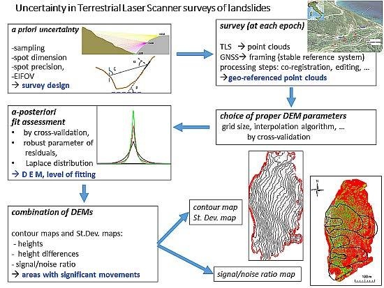
In our paper, the analysis of uncertainty related to TLS surveying is performed considering a typical survey of a landsliding slope as a study case. We discuss, in this context, some sources of errors that can be expected within the survey design and we face the critical issues of data processing to move from points cloud to DEM, such as the choice of interpolation algorithm and its parameters, suggesting a robust statistical parameter to support this choice.
We pay special attention to the realization of a grid of the uncertainty values to associate with the grid-DEM of heights, therefore, making it possible to associate a degree of uncertainty even at quantities derived from DEMs; for example, geo-morphometric features or mass displacements observed in the monitoring, over time, of the slope. With these additional data geologists, geotechnicals, and geomorphologists who have to interpret the characteristics of the landslide have the opportunity to evaluate the significance of shapes and variations that are provided by surveyors.
2. Case Study and Survey
Whatever the goal of the specific survey, it is mandatory to design it correctly by considering the characteristic of both the area (in terms of morphology, extent, etc.) and surveying instruments. Regarding data processing, many other factors should be taken into account, such as the vegetative cover, because editing is often necessary. Furthermore, if the goal is to monitor ground deformations over time, two or more DEMs must be compared in order to compute the displacements of the points belonging to the terrain surface. In this case, one needs to frame all surveys in a single geodetic reference system that is stable over time.
In this work, we have analyzed the reliability of the entire process, starting from field surveys, down to data processing on a test case. Our test case concerns a typical survey of a mountainous area affected by a landslide. Since the purposes of surveying are morphometric analysis and monitoring over time, it is very important to assess its accuracy and precision.
2.1. Case Study
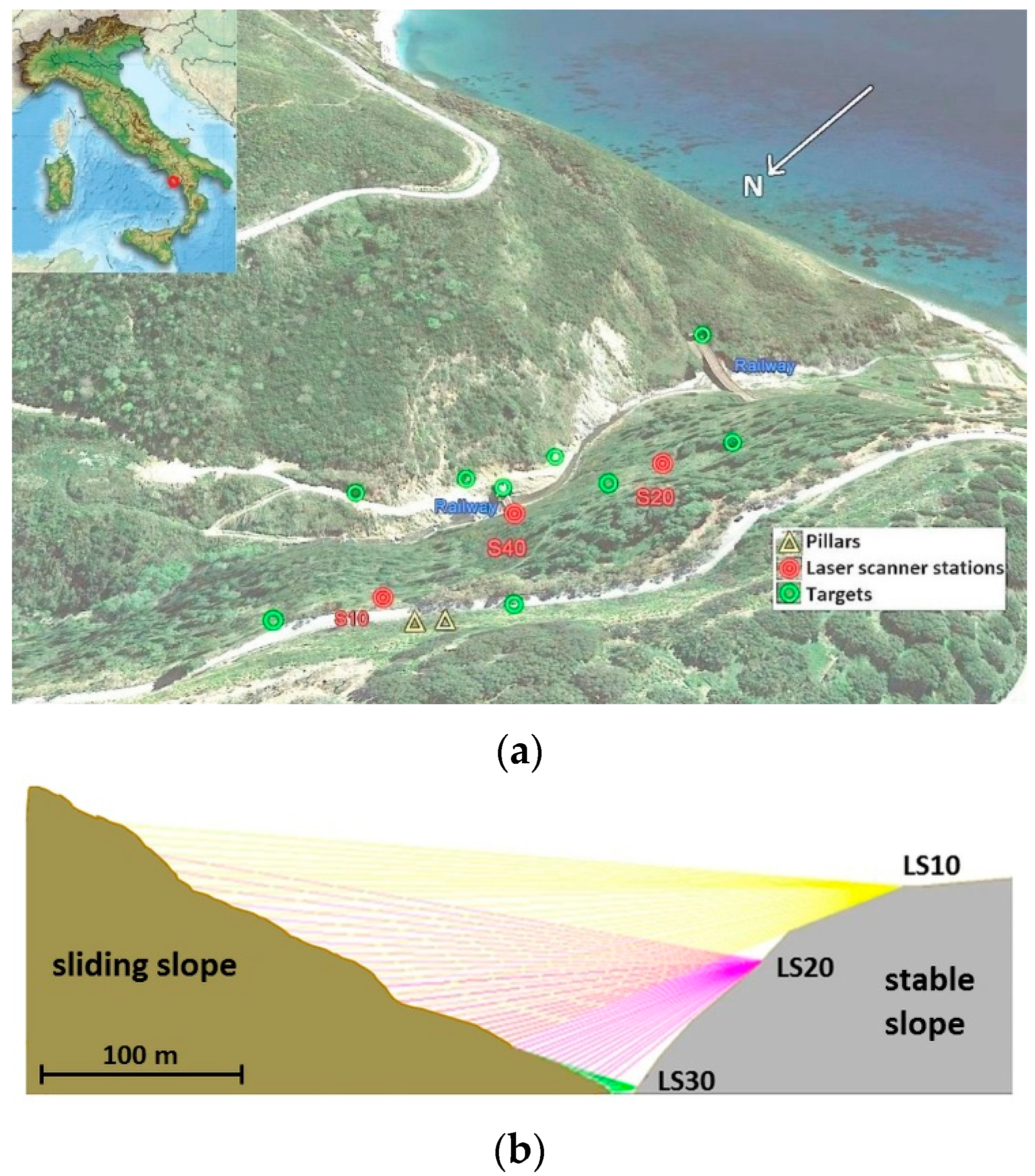
The phenomenon we are monitoring is located in Pisciotta municipality in the Campania region, Southern Italy (
Figure 1a). The landslide has a size of about 500 m east–west, and 400 m north–south, and affects a stretch of road and two railway tunnels with heavy traffic (in both north–south and south–north directions). Among them, the most exposed to landslide movements appears to be the northernmost tunnel because it intersects with the central part of the landslide toe. From a geological point of view, in accordance with the widely accepted Cruden and Varnes’ classification of landslides [
37], the active Pisciotta landslide is defined as a landslide compound system with a deep-seated main body affected by long-term roto-translation, and slow displacements [
38,
39].
The vastness of the area, the high gradient of the slope, the presence of vegetation and the difficult access make it very complex both with respect to the survey design and the execution.
The first survey of the phenomenon has been conducted with a total station and the control points positions referred to a couple of pillars [
40]. The results of the periodic surveys showed that the amount of planimetric displacements in a period of about four years is about 7 m, while the altimetric ones were in a range between 2.5 m and 3.5 m. The average horizontal daily speed of the landslide was approximately 0.5 cm/day, with peaks up to 2 cm/day. In elevation, this resulted in displacements of approximately 0.2 cm/day, with peaks up to 1.5 cm/day.
These operations allowed a first estimate of the magnitude of the ground movement, although the topographical surveying of a small number of points along the road does not allow a quantification of the volumes of material in the landslide or to delimit the area affected by the phenomenon.
2.2. Survey Design and Field Campaign
In order to obtain a 3D numerical model of the landslide slope and its variation over time, we run a number of field campaigns using the terrestrial laser scanning surveying methodology [
40,
41]. A stream separates the two flanks of the valley: the right one is considered stable, while the left one is unstable. From the top of the stable part, the toe of the landslide cannot be seen. On the other hand, the slope toe is of great interest because in this area the slide debris accumulates. The TLS scans should, therefore, be acquired from multiple stations placed both on the upper part of the stable slope, from which the visibility toward the opposite site is very wide, and at the bottom, in order to make a very detailed survey of the lower part.
In all survey campaigns, we recorded laser scan measurements from several TLS stations, located on the stable slope at different altitudes, in order to measure both the upper and the lower parts of the landslide body. In order to survey the upper region of the landslide area the laser stations have been located at a few points on the stable side facing the landslide, several hundred meters away. At the toe of the landslide, there is a railway bridge connecting the two tunnels, and the terrain above the tunnel gate can be measured with high accuracy; not far from this, toward the valley, there is a longer bridge and another tunnel. Here, distances are smaller and short range instruments can be used, obtaining a larger density of points.
We carried out a TLS “zero” survey and about four months later a repetition measurement using a long-range instrument, an Optech Ilris36D, (Teledyne Optech, Toronto, ON, Canada) a further surveying campaign was carried out one year later by using two different instruments; a long range (Riegl VZ400, Riegl Laser Measurements Systems GmbH, Horn, Austria), and a medium range one (Leica Scanstation C10, Leica Geosystems AG, Heerbrugg, Switzerland). The last campaign dates back to June 2012. Here we used both Optech and Leica instruments.
In this paper, we are particularly interested in the data acquired by the Optech instrument in the 2012 campaign; for the purpose of monitoring the terrain displacements, we also considered the Riegl 2011 data.
Figure 1a shows a perspective view of the study area and
Figure 1b shows the scheme of the lines of sight from the different TLS stations. The positions of pillars, TLS stations, and targets are marked with yellow, red, and green symbols, respectively. The mean distance from the TLS stations to the landsliding slope is about 200 m.
In order to frame the whole survey, the target coordinates were measured by GNSS (Global Navigation Satellite System) instruments in static mode keeping fixed the pillars used for traditional survey. The two pillars were, themselves, connected to two permanent stations (PSs) belonging to the IGS (International GNSS service) global network or to its local (national) densification, whose coordinates are known in a geodetic international frame. Due to the significant distance between the landslide area and the PSs, about 30 km far away from the landslide, we made continuous daily GNSS observations.
The strong dynamics of the landslide implies that the measurement campaigns have to be carried out in a very short period of time. This is why we ran both the TLS and the GNSS survey during the same day. Each surveying campaign lasted 2–3 days.
2.3. Data Elaboration and Frame Accuracy
In each survey campaign, we have acquired three to four scans taken from different stations. The first phase of data elaboration aims at determining the positions of both targets and TLS stations in the selected reference framework. The first step of the process is the connection between the permanent stations of the NRTK (Network Real Time Kinematic) network taken as fixed points and the two pillars.
The second step concerns the connection between both targets and laser stations and the pillars assumed as fixed. The “final” coordinates of the targets came from a least squares adjustment in ITRF05 (International Terrestrial Reference Frame 2005).
Table 1 shows the mean values (in centimeters) obtained for the standard deviations (St.Dev.) of the adjusted coordinates of the two pillars and a summary of the values obtained for the standard deviations of the targets.
The subsequent processing of TLS data followed multiple steps: scan alignment, editing, and georeferencing.
Alignment of overlapping scans is a very crucial step to achieve a good metric quality of the output. This task is mathematically operated by using a six-parameter rigid-body transformation. In the first phase, a pre-alignment was obtained from the manual selection of a few corresponding points; we used both natural points and targets as tie points. Then, a best fit alignment was carried out with the least squares Iterative Closest Point (ICP) algorithm [
42,
43].
The resulting scans have to be edited in order to remove from the dataset all of the points not belonging to the bare soil; in our application this concerns essentially the vegetation, but also artifacts. For example, the points inside the tunnel have to be removed from the dataset.
Every single scan has been manually edited (by Pdfedit.exe, a PolyWorks application). The point cloud has been cut into “strips” and then visualized in profile, allowing us to easily identify, select, and manually delete the points above the terrain surface. Such a procedure is very time-consuming, yet the result is quite accurate. The thinner the strip, the better the result.
Once an overall cloud that represents the bare soil is available, it has to be registered in the chosen absolute reference system by means of the target coordinates. We made a six-parameter rigid body transformation in order to georeference all of the scans; a seven parameter Helmert transformation gives almost the same results: the values of the rotations (in decimal degrees) are equal up to the fifth decimal digit, the values of the translations differ by a few millimeters (1 to 5) and the scale factor is equal to 0.99986.
We note that, usually, laser data processing software packages do not provide a rigorous analysis of the quality of the standardized residuals of the transformation. The georeferencing process has led to values of 3D residuals ranging from 5–6 cm. In order to more easily separate the planimetric from the altimetric components, we transformed geocentric coordinates in the UTM_ITRF05 cartographic system.
For the altimetry, we continued to use the ellipsoidal heights. We eventually made a further global alignment of the point clouds at different times by using some recognizable features that have not undergone significant shifts over the period considered, i.e., the rail tunnels. The global alignment process gives values of the standard deviation of the residuals of 2 cm in magnitude.
Once these steps have been conducted, two point clouds that describe the landslide surface at two different epochs are available. Since all surveys have been framed in the same reference system it will be possible to compare the elaborated DEMs, starting from the point clouds obtained at different times.
3. Sources of Errors in TLS Processing: A-Priori Evaluations
In terrestrial laser scanning survey of a landslide, a constant angular sampling step is used, even if the distance between the TLS station and the various parts of the slope is highly variable. This leads to changes in spot size and point density, in the nominal precision of the point positions, and in the actual resolution (in terms of EIFOV).
Data knowledge, in terms of accuracy and density, in relation to the morphology, is important in order to choose the most appropriate interpolation strategy for DEM generation. Of course, many other factors may affect the precision of acquired point data, such as the characteristics of the atmosphere, the soil reflectivity, and the presence of vegetation [
17,
27,
44], but these features are very difficult to handle in mathematical terms. Therefore, the accuracy of surface reconstruction also worsened.
It is possible, instead, to advance some considerations on the basis of both the instrumental nominal accuracy in measuring distance, the azimuthal and zenithal angles, and on the ground sampling distance. Some parameters are a function of the distance of the points from the TLS station. In order to compute this distance, the points of each cloud have been associated with a station identifier. The association remained the same both in the alignment and georeferencing steps in order to be able to compute the distance from the corresponding TLS station for each point. Due to the overlap between two adjacent scans, which is required for scan alignment, some areas’ neighboring points have been acquired from different stations and are located at very different distances. The distance between the scanner and the object affects a number of point “features”, such as nominal position accuracy, spot size, EIFOV, and density, which we will discuss in this section.
3.1. Point Precision
TLS manufacturers give indications of the nominal accuracy of the position of the laser beam center. Fact sheets report RMS (root mean square) of azimuthal angle (), zenithal angle (), and distance () measurements; starting from these values it is quite straightforward to compute the co-variance matrix of the position of each point of the final cloud.
Since the coordinates of the TLS stations are known, it is possible to compute the components (x, y, z) of the vector between every georeferenced point and the relative station.
Values of distance and angles can be easily derived from the vector components:
If we considered the covariance between the variables is null, and we assumed the error in distance measurements are proportional to it by a factor of
kd:
σd =
kd ×
d the associated co-variance matrix is:
By considering the relation between 3D polar and Cartesian coordinate systems and the Jacobian of the transformation:
It is possible to compute an estimated value of the co-variance matrix of the position of a generic point belonging to the cloud by applying the variance propagation law:
From the co-variance matrix it is then possible to extract one-dimensional quantities which are easily graphically representable, such as: σz (rms in height component) or .
In overlapping areas, neighboring points may be located at very different distances from the respective TLS stations and, therefore, their precision is different.
3.2. Spot Size
The uncertainty of the nominal position of acquired points is related to the “center” of the laser beam, whose width is another specific feature of the instrument. The distribution of the radiance along a cross-section of a laser beam is typically Gaussian. The conventional beam diameter encircles 1/e
2 of the total beam power. The radius of a plane section at a distance d is expressed by [
45]:
where
wo = the smallest spot diameter (diameter at the waist) and
λ = the laser beam wavelength.
At great distances, the trend of the normal section of the radius value can be approximated as a linear function of the distance [
18,
19]. For the Optech Ilris3
6D results
wo = 12 mm and
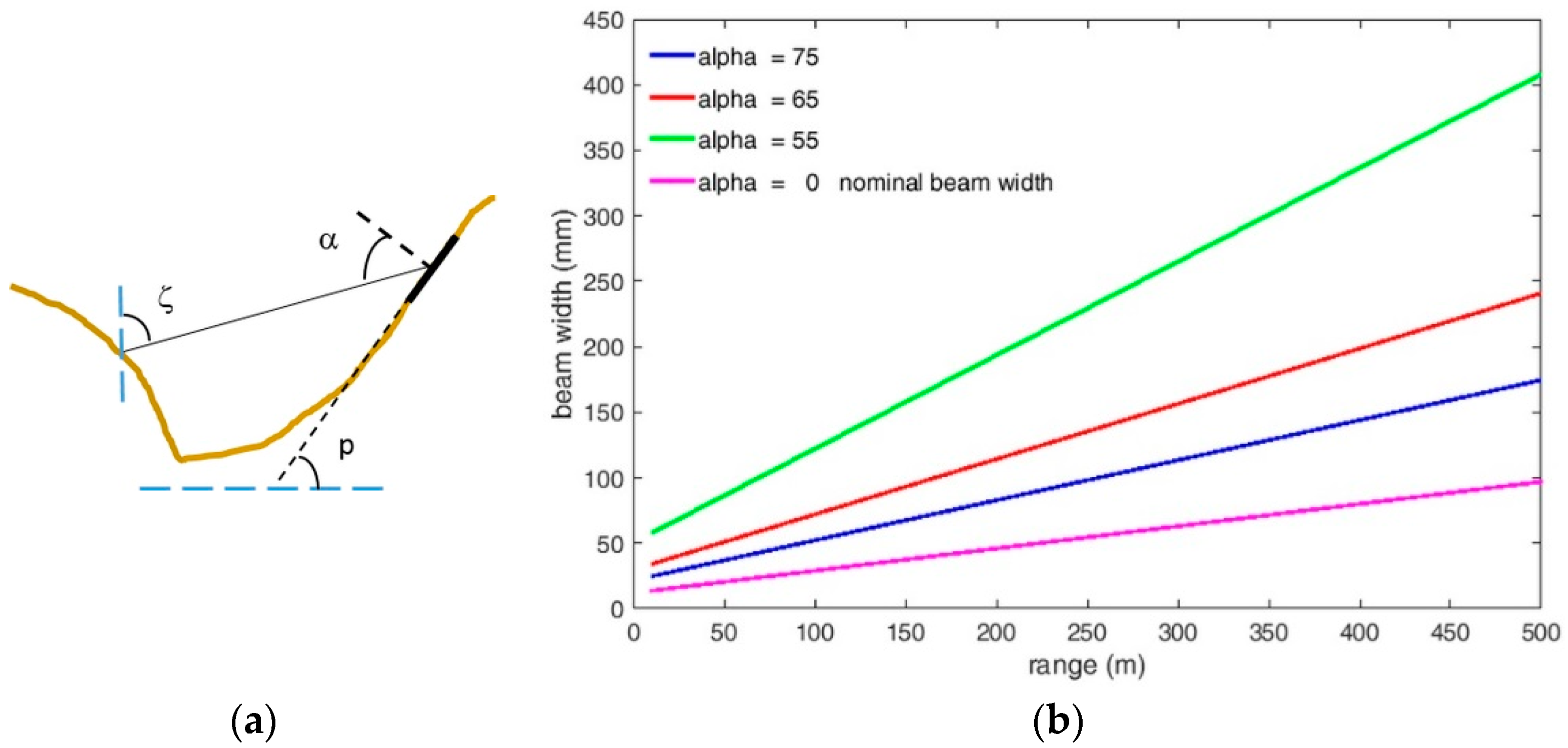
γ = 170 μrad. The spot radius computed at a certain distance with the above formulas must be intended as referred by the cross-section orthogonal to the axis beam, while the effective shape and dimension of the spot on the imaged terrain depends, in general, on its slope with respect to the beam direction; the average slope in the study area obtained by linear interpolation of the surface profile is about 25°. The value of angle α between the normal to the beam axis and the surface may be easily evaluated by means of geometric considerations;
p being the angle between the surface and the horizontal, the angle α is a function of
p, the beam zenith angle
ζ, and the effective beam width (
Figure 2a):
Figure 2b shows a graph of the values of the spot width as a function of the distance between the TLS station and the terrain for some inclination angle values.
These results show that the nominal beamwidth, computed by the product of beam of divergence by distance (that gives the value of the radius of the circumference orthogonal to the beam direction) is definitely an underestimate of the real spot dimension.
3.3. EIFOV Evaluation
The actual resolution capability, i.e., the ability of a TLS to detect two objects on adjacent lines-of-sight, depends on both the sampling step Δ and the laser beamwidth. If the sampling step is much smaller than the beamwidth, then a reliable evaluation of the spatial resolution is necessary. Lichti et al. [
19] examined these issues with the aim of estimating the effective instantaneous field of view (EIFOV). It is possible to compute the EIFOV starting from the average modulation transfer function (AMTF) formula, which contains the beamwidth and the sampling rate:
The contribution of the terms
and
(that state for quantization) causes only minor modulation reduction [
19] and so they have been considered as negligible in our computation.
Assuming for the critical frequency
fc the value of the frequency for which AMFT reaches an amplitude of 2/π, we obtain the expression:
In order to have a more realistic estimate of the effective spatial resolution, EIFOV must be computed taking into account the real spot size on the ground. The error parameters which were hitherto computed are related to the individual beams. We are able to compute them, at least partly, once all of the features useful for design of the survey campaign are known (laser station positions, sampling intervals, etc.). Obviously, the presence of vegetation requires editing to accurately filter the vegetation from the DSM in order to obtain a DTM that properly describes the surface shape.
4. A-Posteriori Uncertainty Evaluations
TLS data are usually characterized by a heterogeneous point density, which represents an important parameter in reconstructing a surface because it affects the interpolation reliability. Point density is a function both of the distance between the TLS station and the terrain and of the adopted angular sampling. Furthermore, we must also consider that, in overlapping areas, the density is greater due to the distance.
In addition to these theoretical considerations, point density certainly depends on a number of local surface characteristics, such as the varied morphology of the slope; thus, some areas are hidden and, in the case of vegetation, must be removed by editing. Heterogeneity in density represents an important parameter to consider in DEM generation because it affects the choice of the interpolation method and the setting of its interpolation parameters (such as search radius and minimum required number of points to use).
To compute the density we used the “point density tool” of ArcMap because it allows considering a square neighborhood corresponding to the DEM cell size. On the contrary, kernel based algorithms spread the computation over a wider circular neighborhood and so tend to smooth the output density raster [
46]. To define the processing parameters, we set the same extent of the DEM and assigned the value of the DEM cell size—one meter—both to the cell size and to the cell neighborhood. Each output raster density cell coincides exactly to the grid cell size of the DEM since the two grids share the same extent and spacing. In this way, the computed density, expressed in points per square meter, corresponds to the number of points present in each cell of the DEM grid.
To create a DEM from a TLS point cloud, several interpolators are available, whose effectiveness relies on the specific features of the input data (e.g., spatial evenness and density variability) and of the required output product.
Once the proper interpolation algorithm is chosen, it is necessary to set its parameters (e.g., spatial grid, search radius and shape of the kernel, number of points inside the kernel, etc.). In our case study, in order to perform map algebra operations on grids we considered it worthwhile to use raster DEMs rather than TINs (Triangular Irregular Network). Therefore, the choice of the DEM grid size is very important.
4.1. DEM Grid Size
Cell size, which corresponds to the distance between two adjacent nodes of the grid, is usually chosen by the user and should depend on the quality and density of the input data [
22,
47], on the extension of the area to be mapped, and on the accuracy required for the output data [
48].
According to McCullagh [
33], the number of grid nodes should be approximately equal to the number of input points, whatever surveying technique is used (ground survey or aerial photogrammetric survey), while Hu [
49] suggests that, for airborne LiDAR data, the cell size S could be estimated as:
where
n is the number of terrain points and A is the covered area. In the case of surveys of large areas, the TLS point cloud is made up of a very high number of points, and with a high variability in density. The “average value” is computed by considering an area of 10 Ha and a dataset containing eight thousand points is equal to around 0.1 m according to the above formula. This value does not appear suitable for use for the whole area.
The choice of the grid resolution, apart from being strictly tied to the original point cloud density acquired from TLS, could also be related to a cartographic concept. Cell size can be closely related to the level of detail of a map, which, in cartography, is often related to the concept of map scale [
34]. A simple criterion for defining the proper cell size of a DEM built with data acquired from TLS data could be verified if the vertical map accuracy standards provided at a certain scale are respected. Given the high density of the input point cloud, we considered only large and medium map scales, from 1:500 to 1:5000.
According to USGS (United States Geological Service), ASPRS (American Society for Photogrammetry and Remote Sensing) and INSPIRE (Infrastructure for Spatial Information in the European Community) recommendations and standards, vertical accuracy is tied to the contour interval, conventionally set to be equal to 1/1000 of the map scale. Furthermore, according to the National Standard for Spatial Data Accuracy (NSSDA) [
50], the vertical accuracy of a data set (accuracy(
z)) corresponds to the root mean square error (
) of the elevation data.
The
is defined as the square root of the average of the squared discrepancies, which, in this case, are the residuals in elevation values with respect to a “ground truth” which can be represented by another terrain surface [
22] or by an independent survey of higher accuracy [
51].
Table 2 shows the vertical accuracy specifications provided by the before-mentioned agencies expressed as a function of the contour intervals usually used for some map scales.
For USGS, the vertical error threshold is set equal to the half of the contour interval [
52,
53,
54].
For ASPRS, the accuracy standard depends on the map class [
51,
55]. For Class 1 maps (highest accuracy) the limiting
is set at one-third the contour interval; for Class 2, at two thirds.
For INSPIRE, vertical accuracy must be consistent with both the contour line vertical interval and the type of terrain [
56].
Table 2 also reports the grid cell size prescribed by ASPRS in relation to the contour intervals [
57]. Since, usually, independent background datasets are not available, the most commonly used method is to compare interpolated elevation values from the DEM with a group of check points or with a subset of the original points withheld from the generation of the DEM.
Moreover, the United States National Map Accuracy Standards (US-NMAS) [
53,
54] establishes that the vertical accuracy, as applied to contour maps on all publication scales, should be checked over a sample made up of the 10 percent of the input data.
4.2. Cross-Validation and Residual Statistic
Cross-validation is a standard method of estimating the goodness of interpolation to fit the surface. Given a data sample made up of a certain percentage of data points (1 percent in our test case), it has been created from a DEM using the remaining points and computed the change in elevation of the single point with respect to the height of the corresponding cell of the DEM.
In our analysis, data points have been excluded from the control sample one at a time or all at once. We have run a number of tests using different interpolation methods and different parameters. The probability density function of the residuals is never Gaussian since, for example, it is characterized by a higher value of the kurtosis.
Figure 3 shows the frequency distribution of residuals obtained after cross-validation of the elevation data used to create the DEM with respect to the 1% sample data.
In the figure, the red line represents the trend of the empirical probability density function (pdf), while the blue line represents the trend of the pdf of the random variable distributed normally with the sample mean and standard deviation.
The normal distribution does not fit the empirical trend well, whereas a Laplace distribution, also called a double-exponential distribution, describes it better. The general formula for the probability density function of the Laplace distribution is:
where
μ denotes the location parameter, and
b denotes the scale parameter. This distribution is symmetrical (skewness = 0), with a variance of 2
b2 and excess kurtosis of 3. Laplace distribution has already been applied in [
58] for the error analysis of a DEM obtained from ALS data, with GCPs measured by GPS.
The
μ and
b parameters can be estimated directly from the sample data through the mean and mean absolute deviation, respectively [
59]:
In order to evaluate the goodness of fit for these distributions to the sample data, we performed a Kolmogorov–Smirnov test:
The test statistic is the maximum absolute difference between the empirical cumulative density function (cdf) computed from the sample and the hypothetical cdf:
where
F(
x) is the empirical cdf and
G(
x) is the cdf of the hypothetical distribution.
4.3. Data Characterization via Variograms
Data knowledge, in particular with regard to spatial regularity, plays an important role in choosing the most appropriate DEM interpolation algorithm and its parameters. With this aim, it is useful to analyze the empirical variogram that provides a description of how the data are related (correlated) to distance. The mathematical definition of the semi-variogram is:
where
E{ . } indicates the expectation operator and
γ ( . ) results in a function of the separation distances between points (Δ
x, Δ
y).
Given all of the N pairs of point clouds:
IΔ (Δ
x, Δ
y) = {(
i,
j) | (Δ
xi,j, Δ
yi,j) ~ (Δ
x, Δ
y)}, the experimental semi-variogram
g(.) for a certain separation vector (Δ
x, Δ
y) is computed by averaging one-half of the difference squared of the
z-values over all pairs of observations separated by approximately that vector [
60]:
If we consider an isotropic distribution of points,
g(.) depends only on the distance between points:
In the construction of a variogram, computing time is highly dependent on the number of n sample points because the number of pairs used to compute every empirical value g(Δx, Δy) grows quickly with n.
The elaboration of such a large number of point pairs is a time consuming process even for a powerful computer; therefore, it may be convenient to perform a decimation of the sample data points, reducing their number by a factor of five, 10, or even 20. A high decimation factor (e.g., 20) causes a further decrease in density in those areas where the point density was already low, whereas it has very little influence on density where the density was initially high. Therefore, a strong decimation of data can be done in high density areas, whereas in low density areas it is better to use all of the points.
The empirical variogram can be computed for a number of lag distances chosen directly by the user. The functional model should realize a good fit of the empirical data; Gaussian, power, and all of those that solve the kriging equation are allowed. In our test case, a preferred direction of gradient is noticeable. The trends in the empirical variograms depend on what direction is considered, if along the river channel (almost corresponding to the north direction) or along the direction of greatest slope (east direction). This makes data modeling more difficult, but allows us to define an empirical value for anisotropy.
4.4. Interpolation Method
Several algorithms can be used for DEM interpolation (inverse distance weighted, natural neighbor, rational base function, etc.). Their effective ability to faithfully reconstruct the surface depends on both the characteristics of the input data and the morphology of the terrain to be modeled. In order to choose the best algorithm to interpolate our data, we used cross-validation over a sample of 1% of the input data; we then analyzed the statistical properties of the residual distribution, in particular the median absolute deviation (MAD).
The width of the search interval (the elliptical to take into account the anisotropy quantified by the variogram) can be chosen so as to have a sufficient number of points in the neighborhood of the node also in the less-dense area, along with the parameter that allows us to set the number to a maximum of points to consider. In high-density areas, we have enough points in a closer neighborhood around the grid node, with positive effects on the structure of the interpolated surface.
The Kriging has the advantage of directly using the information stemming from the variogram. The assigned weight depends on the distance between the point and the DEM node. Furthermore, it is possible to produce an error map which shows the standard errors of the estimates.
The graphical representation of the lines of equal value of standard deviation allows us to locate the boundaries within which the surface topography is respected. Beyond this boundary, the indetermination associated to the estimate makes the DEM-derived products unreliable.
5. Results
To analyze the uncertainties associated to the TLS survey of a landslide, it is useful to disentangle results obtained considering a priori assessments from ones obtained starting from the interpolated DEM.
5.1. A Priori Uncertainty Assessment
The a-priori assessments concern the accuracy of the single point position, the actual footprint size on the surface and the actual resolution.
5.1.1. Point Precision
In this case study, for each point, the precision of the height component
has been computed. This quantity has been interpolated in order to obtain a trend map along the slope.
Figure 4a shows the positional accuracy map obtained by multiplying angular accuracy (80 µrad both for azimuthal and zenithal angles for the Optech instrument) by distance. This so-called positional error has been computed at a confidence level of 99%. Positional accuracy is poor in the upper belt of the slope because it is a function of distance.
Figure 4b shows the map of the trace of the co-variance matrix. The positional error is simpler than the latter to compute, being just a function of the distance and angular accuracy. Note the “salt and pepper” effect due to overlapping scans. The two maps are very similar because the contribution of the height error to the 3D co-variance matrix is not so relevant to make it too much of a difference from the positional error.
5.1.2. Spot Size
Based on the laser beam divergence of the TLS we used, we computed the spot map shown in
Figure 5. Note that the trend of the spot map looks very similar to the positional accuracy map (shown in
Figure 4a), this is because both of the quantities depend on the distance from TLS stations. Even if the positional accuracy is a statistical quantity, and the spot is a deterministic one, it can be said that at a 99% confidence the level positional accuracy is similar to the spot dimension.
The values we showed in the figure underestimate the real values. We could make our estimate more realistic if we knew a reliable value of the slope. In our case, the average slope of the study area is approximately 25 degree.
5.1.3. EIFOV Evaluation
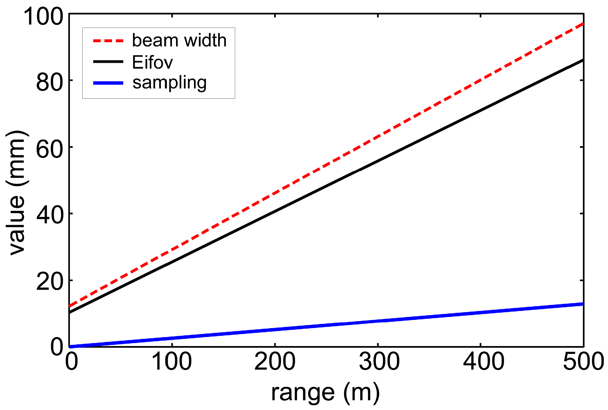
We have computed the EIFOV as a function of the distance, using the values of the parameters set for the measurements.
The survey campaign was carried out using a TLS whose sampling rate both in zenith and azimuth angles was set to a value of: Δ = Δθ = Δα = 26 μrad.
Figure 6 shows the graph of the EIFOV value (in mm) as a function of distance. For the beamwidth, we assumed a value corresponding to the cross-section.
The EIFOV value is very close to the beamwidth. This means that we could achieve the same resolution (in terms of EIFOV) even if we had used a lower sampling rate than that used, meanwhile reducing the blurring effect.
5.2. A-Posteriori Uncertainty Evaluation
Only after alignment, vegetation editing and georeferencing, it is possible to assess the a posteriori level of uncertainty of the acquired point cloud.
The actual density of measured points is one of the most important parameters for the uncertainty analysis, because on it depends the choice of the proper interpolation method and of its relevant parameters.
5.2.1. Point Density
To define the processing extent, we set the same value of the output DEM—one meter—both for the cell size and for the cell neighborhood. Each output raster density cell corresponds exactly to the grid cell size of the DEM since the two grids share the same extent and spacing.
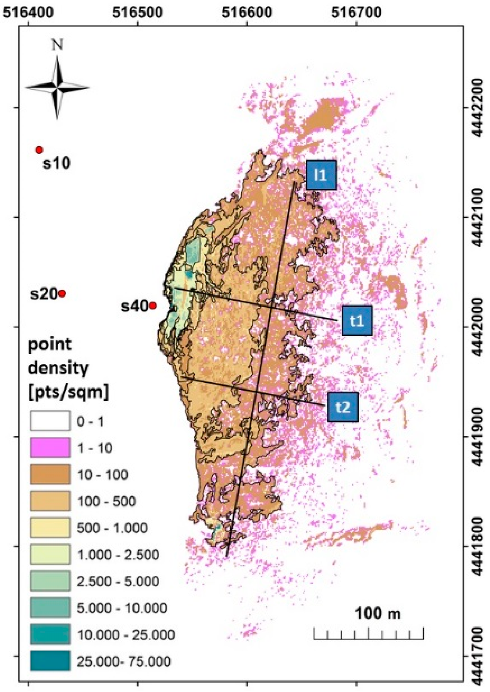
Figure 7 shows the density map produced (number of points/m
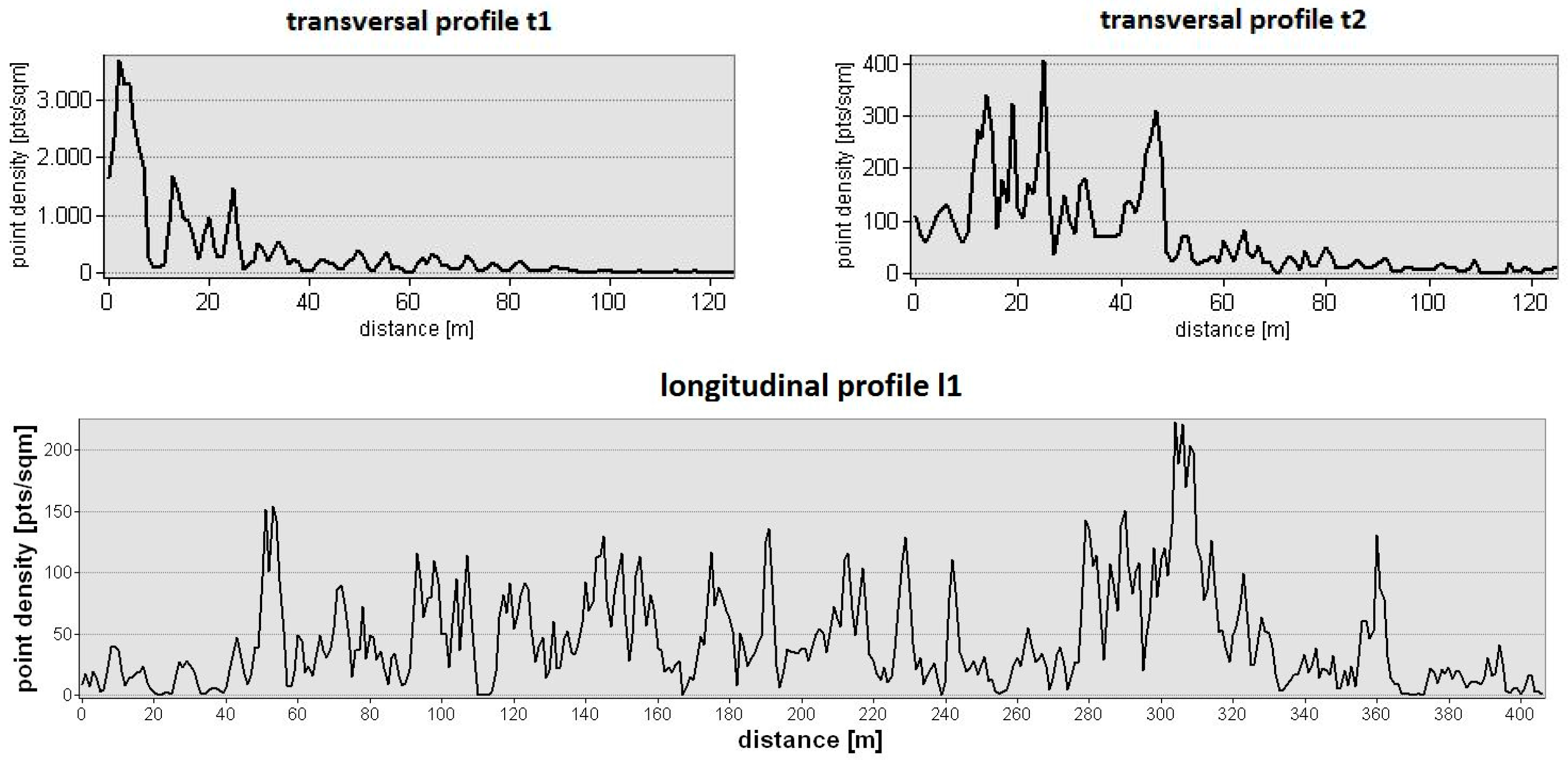
2). As expected, point density is very high in the lower belt of the slope, closest to the TLS stations (they are indicated in the map as red dots). It should be noted that also in the upper belt of the slope the point distribution is not regular at all, with scattered cluster points which are not connected each other.
Figure 8 shows a number of profiles along the lines traced on the map. The high variability in density along the longitudinal profile is due to the non-uniform point distribution on the ground in the upper and middle belts of the slope despite the fact that the angular sampling step was set to a single value for all of the scans. In addition to the density map, other density-related information has also been considered in the choice of space domain parameters for the DEM extraction, such as the number of points within a certain search radius at each node. Regardless of the specific survey characteristics, point clouds obtained by TLS for the different parts of the landslide have highly variable density from each other (of many orders of magnitude, sometimes). This does not happen for either airborne laser scanning or aerial and satellite photogrammetric surveys.
5.2.2. DEM Grid Size
According to specifications given in
Table 2, we randomly extracted from the entire input dataset, consisting in about 8.5 millions of points, a sample corresponding to 10 percent of the data. The remaining 90 percent of points were used to produce a series of DEMs; all of them were built using the same interpolation algorithm (kriging) and search radius (10 m) from the same source data at three different grid spacings: 0.5 m, 1 m, and 2 m.
Later, we computed the differences between the CP elevation values and the corresponding values of the DEMs. The residuals exceeding a threshold absolute value three times larger than the standard deviation of the sample are considered gross errors. Since the value of standard deviation computed for the three datasets is around 1 m, we set a critical value to 3 m. The residuals highlighted that a small number of gross errors are present in our data.
Table 3 shows, for the three tested grid sizes, some summary statistical values referred to the residuals computed on all of the data and on the reduced subset after the removal of gross errors.
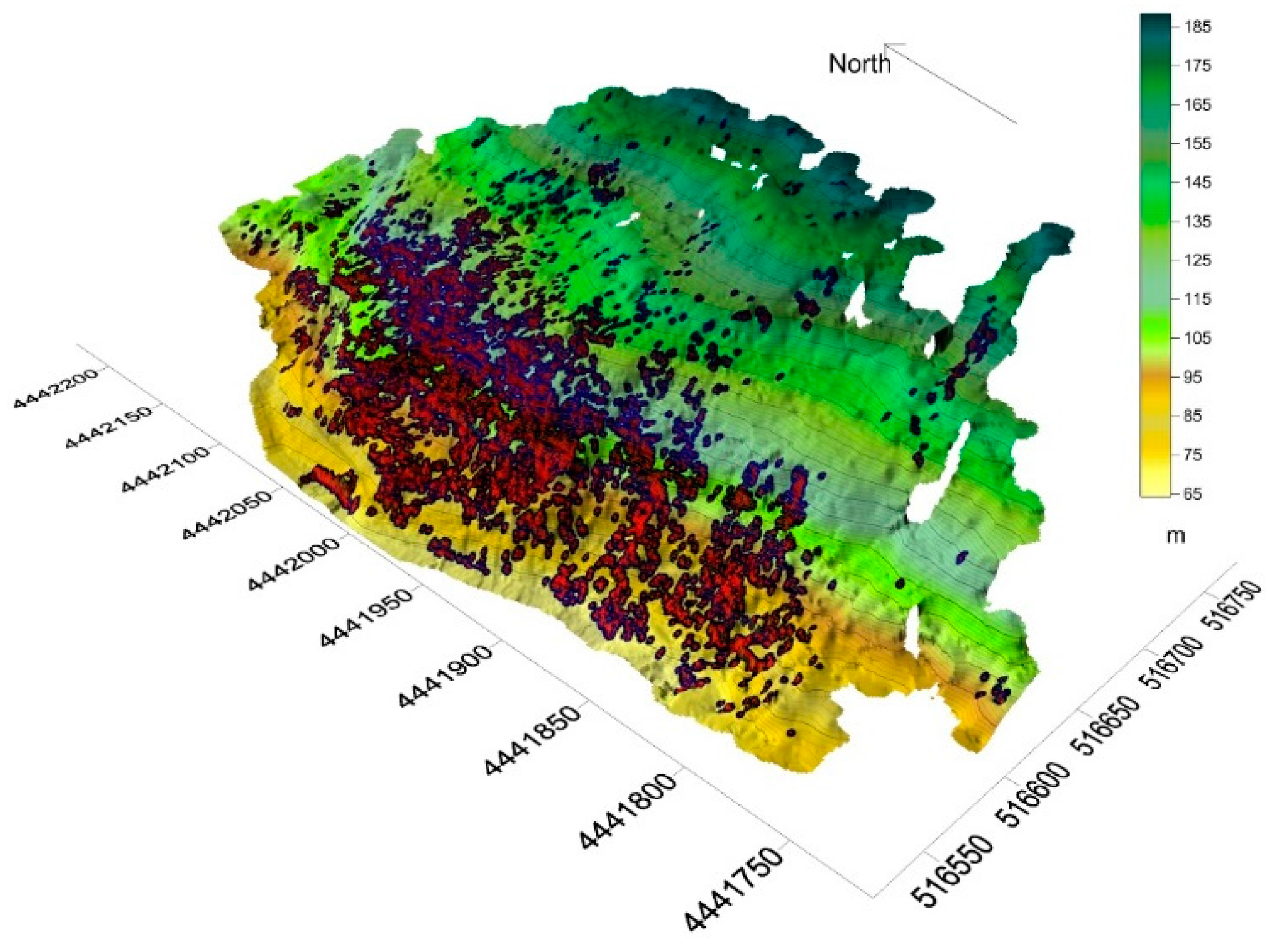
In
Figure 9, the dots show the position of the outliers that have been rejected. Blue dots represent residuals larger than 3 m, red dots represent those smaller than −3 m. Gross errors are mostly present when a sudden change in slope occurs, e.g., at the horizontal (roads) and vertical (railway tunnels) planes. Notice the reduction of the standard deviation of the sample after outlier removal. The value diminished to a little more than half its initial value.
To assess compliance with standards, it has been verified that 10 percent of the residuals fall within the vertical accuracy values shown in
Table 2.
Table 4 shows the results of the analysis of compliance.
In the case of the 0.5 m grid size DEM, compliance with standards is never verified for a map scale of 1:1000. For a 1 m grid size, according to INSPIRE, the standards-compliance is verified only in the case of “undulating” or “hilly” terrain, whereas, according to ASPRS, it is verified in the case of “class 2” or “class 3” maps. Lastly, for a 2 m grid size, the standard-compliance is always verified except for “flat” terrain (INSPIRE) or “class” 1 map (ASPRS).
Hereafter, unless stated otherwise, we used the 1 m grid size DEM, suitable for the production of maps at 1:2000 scale, deemed sufficient for the analysis of the morphometry of a slow-moving landslide like the one we studied.
5.2.3. Cross-Validation and Residual Statistic
We have run a number of tests changing the interpolation method and its parameters. The observed statistical behavior appears quite general given that the statistical results are comparable with the previous ones. In light of the above considerations, we used the median absolute deviation of the residuals in the analysis of the goodness of interpolation to fit the surface. Elevation data used to create the DEM have been cross-validated with respect to 1% of the sample data.
Figure 10 shows the plot of the Laplace distribution with μ and b parameters. The distribution (blue line) fits the sample data (red line) better than the normal distribution. To also take into account the near-zero values, we then computed a further Laplace distribution (green line) with the location parameter
b’, which is a function of the median absolute deviation MAD, instead of
bmean:
This latter Laplace distribution fits the sample data better than the former if the residual values are small (absolute values between 0 and about 20 cm) but still does not fit the empirical trend well for halfway residual values (ranging from 40–70 cm, approximately). In this case, the empirical function is underestimated with respect to the Laplace one.
5.2.4. Data Characterization through Variogram
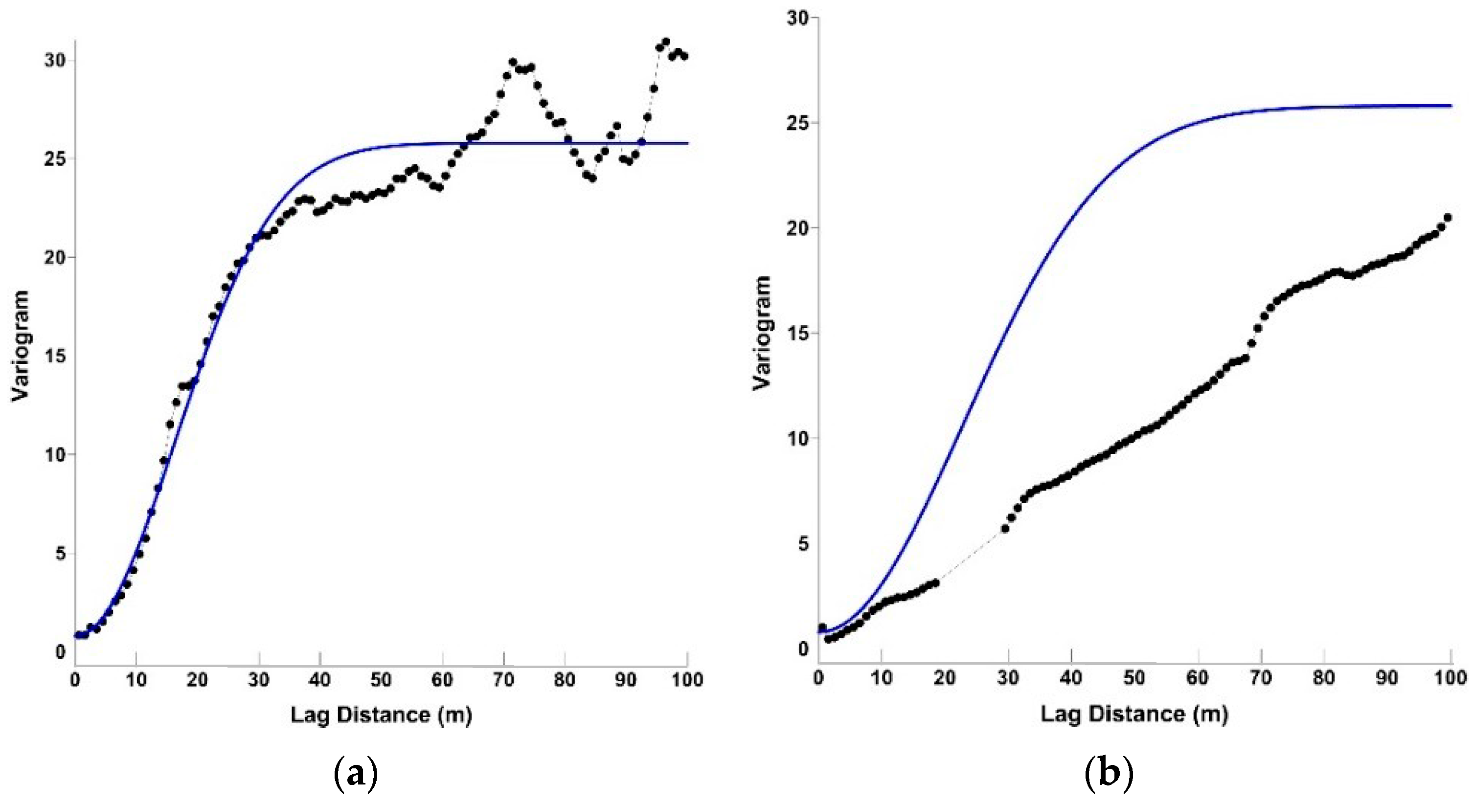
Obviously, the altitude difference between neighboring points in the landslide turned out to be much higher in the direction of the gradient (roughly corresponding to the east direction) than along the river channel and this makes necessary to evaluate the degree of anisotropy through a variogram analysis.
Figure 11 shows the variograms (dotted lines) computed using quite large values of lag (100 m) along both of the direction of the maximum slope (
α = 0° along the east) and its orthogonal (
α = 90° along the north). It is possible to efficaciously fit the variogram model along the east direction, as shown in
Figure 11a, through a Gaussian function of the lag vector
h [
61]:
where
a = (practical) range and
c = sill or amplitude (the semivariance value at which the variogram levels off).
In
Figure 11, the blue line represents the trend function computed with
a = 23 and
c = 25 empirical values.
Figure 11a shows the variogram obtained along the north direction, characterized by
g(
h) values that are much smaller than those along the east direction at the same
h (
Figure 11b). It is clear that, in this case, the Gaussian functional mode adopted for the other direction is unsuitable. The variogram computed with smaller values of lag distances, which are more appropriate with the search radius chosen (20 m), is shown in
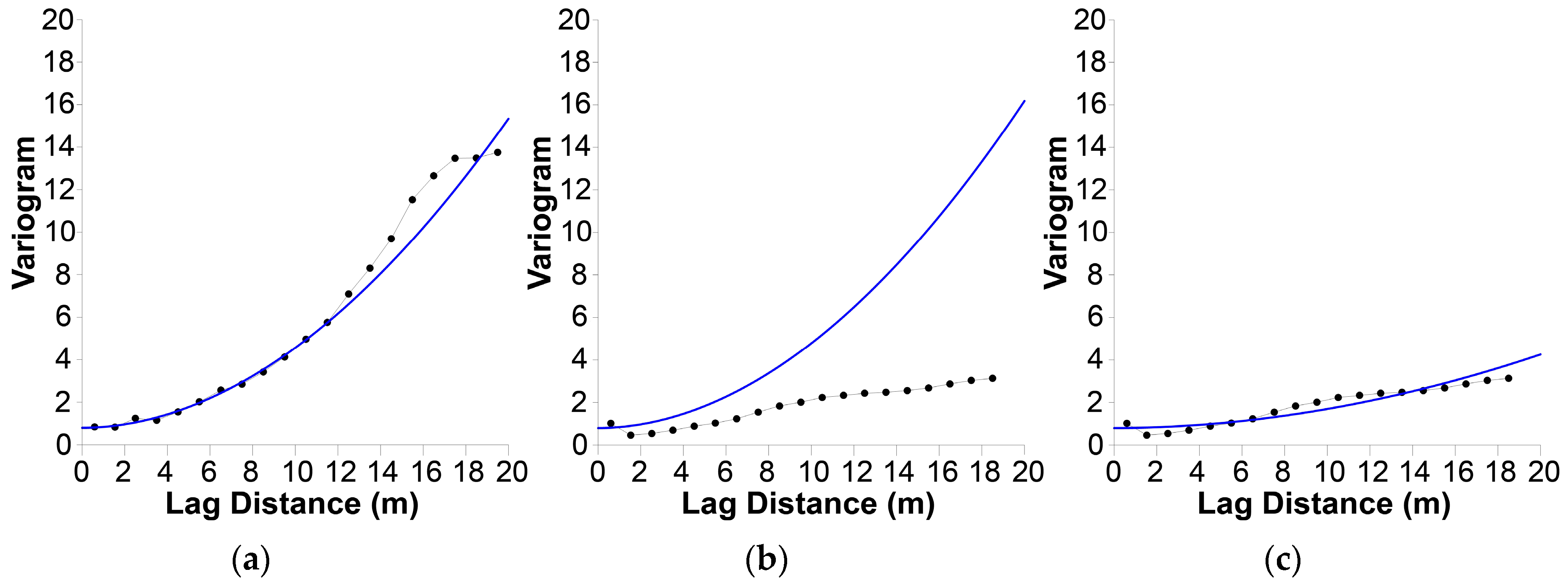
Figure 12.
Here, the model has been computed using an anisotropy ratio of 0.4 and an anisotropy angle of 15°. A nugget effect of 0.8 has been added. More in detail, the model that best fits the variogram in the 0° direction (
Figure 12a) is a power function:
with power parameter
ω = 1.95 along with a nugget of 0.8,
Figure 12a.
Such a model does not fit the empirical variogram computed along the α = 90° direction, along the river channel,
Figure 12b. This confirms the large-scale anisotropy in the data. We use an anisotropy ratio of 0.4 to improve the fitting in that direction. The resulting model fits the empirical variogram data much better than the isotropic model along this direction too,
Figure 12c. We ran a number of experimental tests in order to choose both the model and the values of the parameters; therefore, their choice is partially subjective. The use of specialized application software (e.g., Surfer by Golden Software, Golden, CO, USA) simplifies the user’s choice since the selection process is guided very well.
To summarize the results of our test, we have taken the anisotropy that affects our data into account; thus, we chose an elliptic search neighborhood, with a semi-axis ratio of 0.4. The kriging interpolation method allows us to apply the chosen variogram model directly.
5.2.5. DEM Interpolation and Error Map
In order to choose the best suitable algorithms for the generation of terrain models in terms of befitting and computation time we ran a number of tests.
Table 5 summarizes the most significant results. There are no noticeable differences among these interpolators.
Many authors have chosen to use IDW (Inverse Distance Weighted), whereas we chose kriging not only for the slightly better MAD value and for the possibility of a full use of its variogram model, but especially because it allows the creation of a map of the uncertainty in the interpolation of height values. The weight of IDW interpolator has been chosen equal to the inverse of the squared distance, for this reason hereafter the algorithm will be called IDW2.
Such maps would also be very useful for the assessment of the reliability of the interpolated values.
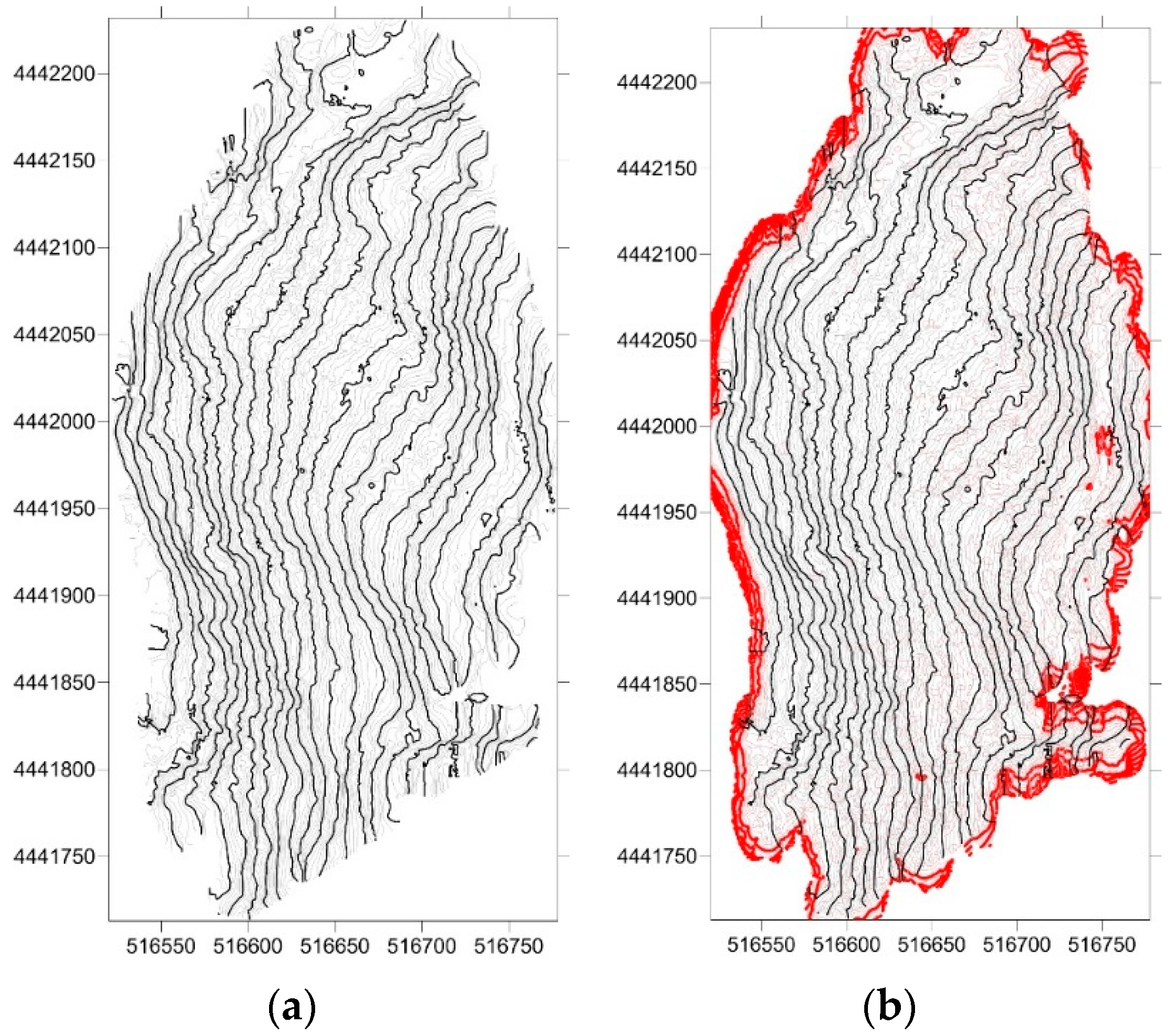
Figure 13a shows the contour lines with a 1 m interval obtained for the test case using the variogram model of
Figure 12;
Figure 13b the plot of the lines of equal standard deviation values on the contour map.
Such a representation allows us to define “objectively” the boundaries of the area to be considered for further analysis. The red curves connect points with a value of the standard deviation larger than 1 m. In cases of higher values, the survey is unreliable. There are points characterized from a high value of standard deviation also inside the area. Border effects are evident.
6. Discussion
During the design phase of a survey it is already possible to estimate, in advance, some important parameters that will affect its precision, such as the positional uncertainty of the beam center, the spot dimension, and the value of the EIFOV, useful for controlling blurring effects. This is possible through straightforward formulas related to instrumental features, given a rough knowledge of the area to be surveyed and once the positions of laser stations are defined.
In our test case, concerning a TLS survey with a sampling rate of 26 μrad, the footprint size orthogonally to the laser beam is of the same order of magnitude as its indeterminacy at a 1% level of confidence, with an EIFOV value close to the spot size. The slope of the landslide with respect to the laser beam direction also has to be taken into account, because it makes the real footprint larger than the normal section of the beam at the same distance; that obviously implies a different EIFOV value.
The actual precision of the survey also depends on many other factors not mathematically predictable a priori: co-registration of scans, global alignment, the survey of targets with GNSS or a total station, geo-referencing of the global aligned cloud and, above, all editing.
The final accuracy of the point position is unknown; the only indicators for accuracy are the georeferencing residuals or the residuals of a few control points not involved in the geocoding process.
Especially in monitoring it is very important to assess the accuracy and stability over time of the points that define the reference frame at each epoch. The use of a permanent GNSS network close to the area to be monitored allows reaching the precision required.
To avoid expensive ground surveys carried out with instruments “more accurate” than TLS, it is possible to use the cross-validation method to evaluate the quality of the fit.
The probability distribution of the residuals, both in our test case and in other samples of data, is quite symmetric with a mean of zero and with the kurtosis much higher than that of the normal distribution. The Laplace statistical distribution better describes the trend of our data; more in detail, the probability function is closer to the sampling one when considering, as the scale parameter, the median absolute deviation instead of the mean absolute deviation.
In order to choose which DEM interpolator, and the associated parameters among the few that are implemented in the software package, better fits the georeferenced point clouds, we have used MAD since it appears to be more robust than the standard deviation in the estimation of the dispersion in the sampling distribution. Among tested interpolation algorithms, the best results have been provided by inverse distance weighting (power 2) and kriging algorithms. We have chosen the latter because it allows the use of a weights model based on the variogram dependent on the input data feature, taking into account their anisotropy, as well.
Another important characteristic of kriging, which makes its choice advantageous with respect to other algorithms, is to allow the computation of a standard deviation map of interpolated heights, thus providing an accuracy assessment of the output DEM. Such a map enables the identification of the areas with smaller standard deviation where the DEM is reliable and can be used to derive geomorphometric parameters.
In monitoring of slope movements, sequential TLS campaigns taken at different times usually do not cover the same area or maintain the same precision. In the common area, it is possible to analyze terrain movements by comparison of multi-temporal DEMs. It is also possible, using simple propagation error formulas, to assess the uncertainty in the evaluation of elevation differences for every node. This computation does not take into account correlations between the heights of neighboring nodes and so should not be considered as a rigorous estimate. In order to perform this analysis, we have processed data coming from a further survey carried out in the same area (slightly wider) one year after using a different TLS (Riegl VZ400). The data processing followed the same steps as previously described.
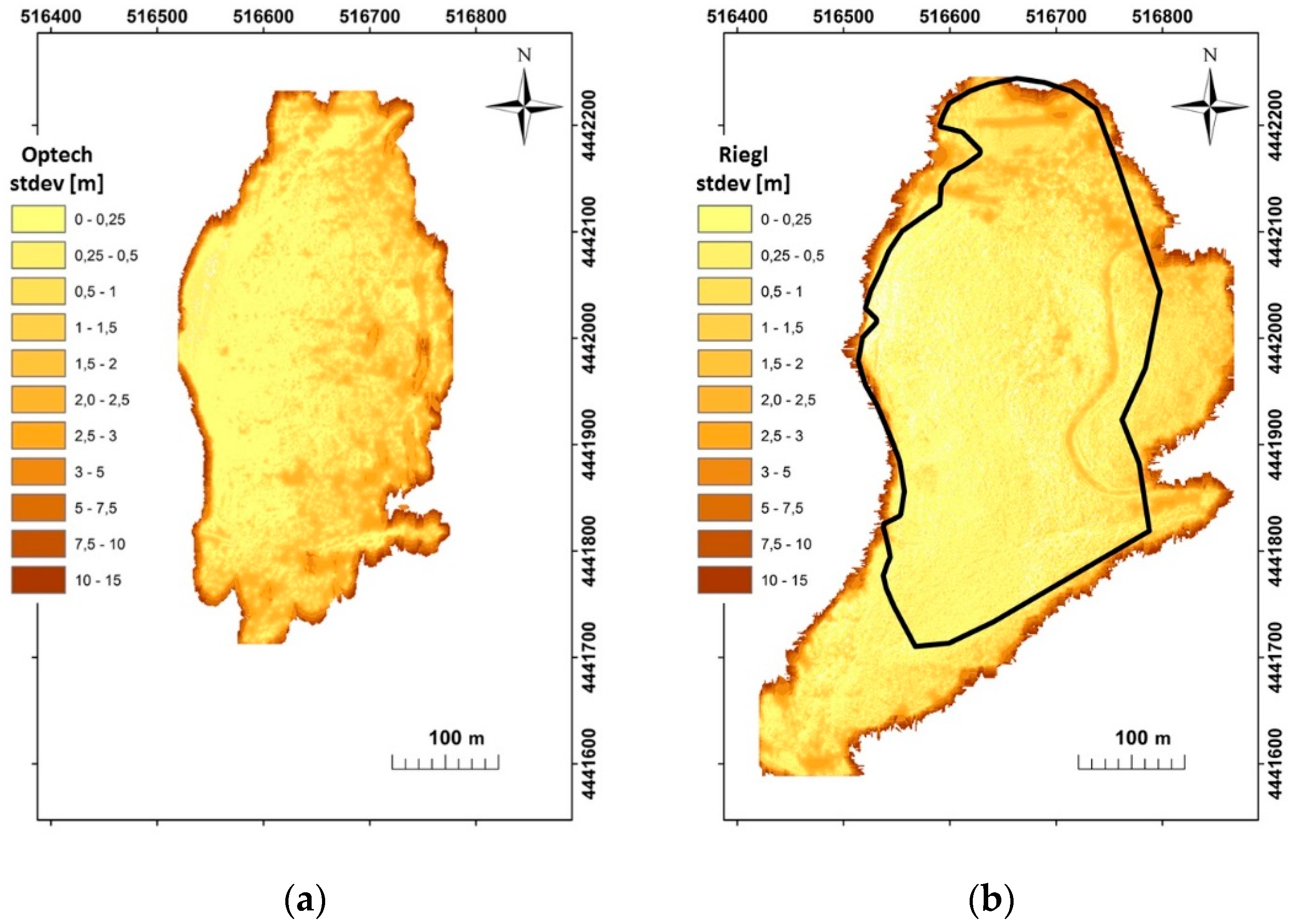
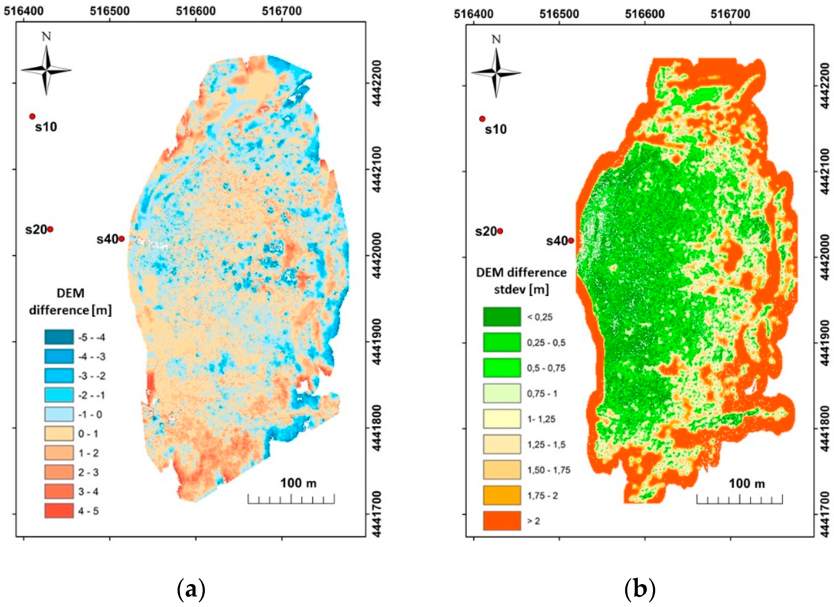
Figure 14 shows the standard error maps of the two DEMs built using the same interpolation parameters for both. The possibility to associate a parameter of uncertainty to the elevation of each DEM grid node made it possible to do the same for the computed height differences (
Figure 14a). This assesses the significance of the mass movements (
Figure 14b). Since we have computed the differences between the elevation values of the Optech survey (the most recent one) and those of the older survey, if the difference between the two values is positive, an accumulation of landslide material occurred and, conversely, an erosion. The area shown in
Figure 15a is that surveyed by Optech, the smaller one.
Propagation of variance has been carried out in a GIS environment using map algebra operators (
Figure 15b). In order to make the maps more legible, residuals larger than 15 m are not drawn on the map; they are centered on the borders of the interpolation surface.
The variance of the difference is strongly affected only by edge effects caused by Optech DEM interpolation, as the Riegl survey covers a significantly larger area (apart from the front of the landslide, located to the west, which is common to both).
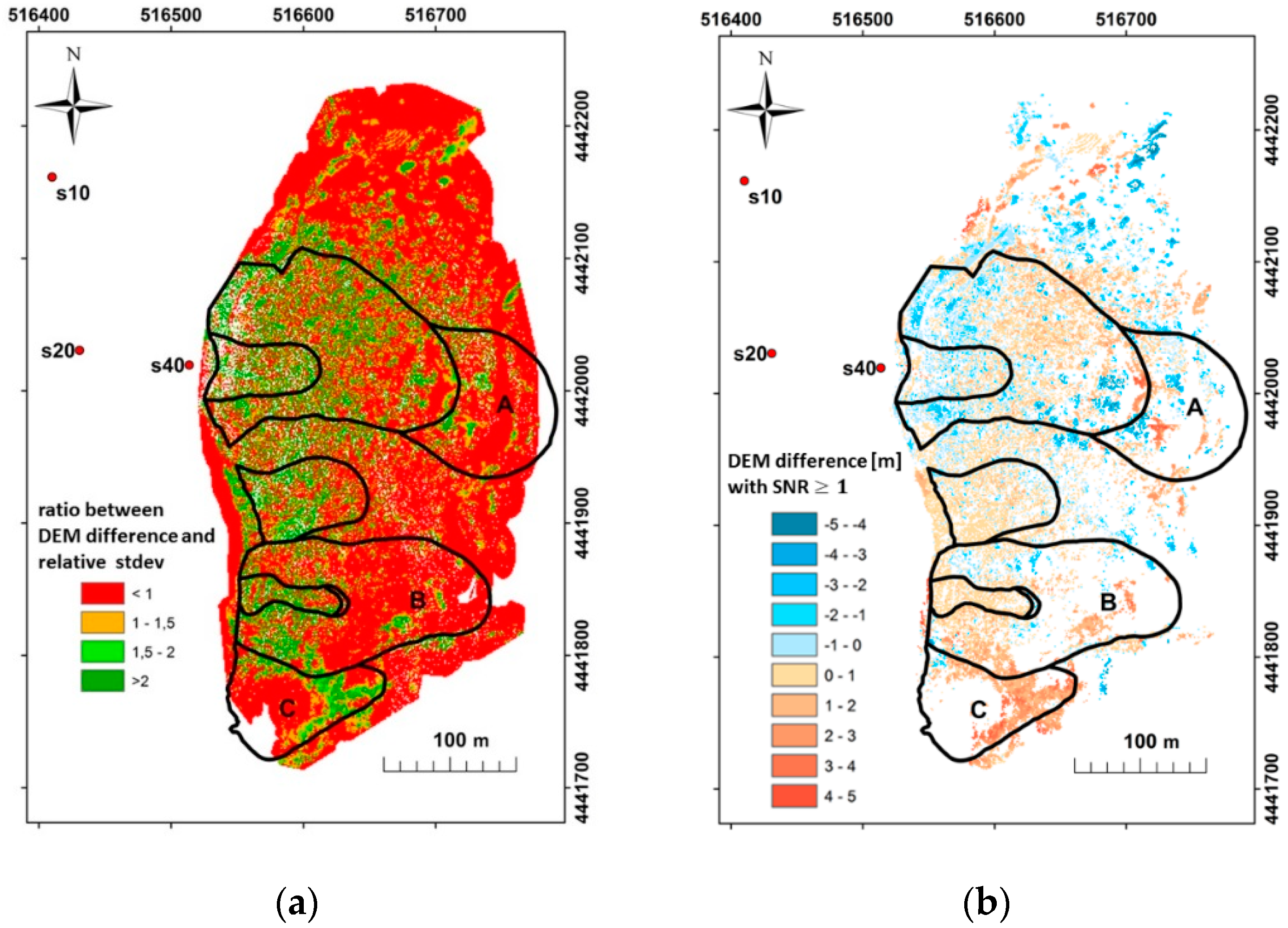
It could be also useful to compute the ratio between the height difference and the relative indeterminacy (
Figure 16a). This index corresponds to a sort of signal-to-noise ratio (SNR). These products are related to the precision of the grid difference once the significance level is defined; they allow the evaluation of the extension of the area where deformation monitoring can provide reliable results. In
Figure 16b is reported the map of the difference between the two DEMs, filtered on the basis of a SNR threshold equal or greater than 1.
The geomorphological analysis of the evolution in time of the individual landslide bodies is usually based on the contour lines. In the figure, the boundaries of the various landslide bodies traced in overlay have been identified by a geomorphologist (see Guida, personal communication) on a contour level map derived from a previous survey.
The portions of the landslide bodies indicate md by the letters A and C are characterized by a signal-to-noise ratio of the DEM differences that is particularly low; therefore, this fact has to be taken into account in further analysis. The SNR of the landslide body indicated by the letter B is critical only in its upper part (east); it is, therefore, advisable to divide it into two in order to take into consideration only the bottom part for reliable analysis.
The analysis of the DEM differences allows also a better delineation of the shape of landslide bodies. For instance, considering
Figure 16b the crown of landslide body C has to be retread upward from the position identified considering only contour levels.
As expected, regardless of the morphology of the slope, the most critical areas for the signal to noise ratio are located where point density decreases because of the distance from TLS stations. The front of the landslide, located to the west, is particularly critical, although here point density is very high, due to the propagation of the border effects of both the DEMs. It is, however, important to notice that the uncertainty associated with the difference of the two grids is significantly worse than expected considering the positional accuracy computed in advance for each scan (
Figure 4). The theoretical accuracy is related to the precision of the instrument and does not take into account either processing steps (alignment, georeferencing, editing), nor the subsequent interpolation of the individual scans to build DEMs and the propagation of errors in their difference.
7. Conclusions
It is possible to estimate the accuracy and the precision of a TLS survey already in the design phase once the general geometry of the area to be surveyed, the position of laser stations, as well as the precision of the TLS to be used are known. In particular, it is possible to compute the laser beamwidth and the uncertainty in the position of acquired points by using simple formulas; they are both a well-known function of the instrumental features and of the distance between the TLS and the ground points. Given a sampling frequency, the EIFOV, which defines the effective spatial resolution of the TLS, can be easily computed.
During the survey a number of additional errors occur, not only due to the TLS measurements, but also to the survey of targets in field and within the point cloud. Usually, the final accuracy is assessed by evaluating only the residuals of the alignment and georeferencing processes.
Actually, it is not trivial to estimate the errors over the position of the surveyed points. An appropriate error budget analysis performed during all phases of the process could help in order to assess the quality and reliability of the survey, as well as the capability of the DEM to represent the elevation of the Earth’s surface.
In order to define the proper cell size of the DEM built with data acquired from TLS data, we related to the cartographic concept that establishes a relationship between cell size and scale map. For a few cell size values, we verified if the vertical map accuracy standards provided at a given scale are respected. The results of our analysis proved that the choice of 1 m grid size DEM is suitable for the production of maps at 1:2000 scale, deemed sufficient for the analysis of the morphometry of a slow-moving landslide, like the one we studied.
To evaluate the accuracy of the DEM, an effective method is based on cross-validation procedures. The statistical analysis of the values of the residuals, namely the height differences between the points of the validation sample and the interpolated surface, allows the evaluation of the goodness of interpolation to fit the surface. One more advantage of the cross-validation method lies in its cost effectiveness because “more precise“ additional and independent measures are not required.
In our study case, a Laplace distribution fits the empirical trend better than the Gaussian distribution. We suggest the use of a robust estimation parameter, such as MAD, to assess the goodness of fit. The analysis of the agreement of the sample distribution with the theoretical one allowed us to make a reasonable choice among various interpolation algorithms and related parameters. Some algorithms, like inverse distance to a power or kriging, provided good results in interpolating the ground points to generate the surface model. Another strong point of kriging work is that the method can employ a model of a variogram that allows taking into account the spatial distribution of the points. In our case study, an unambiguously preferred direction of gradient has been highlighted.
Furthermore, kriging also provides a standard error map that shows the uncertainty related to the predicted height values of each node of the DEM. This error map allows defining, in a more “objective” way, the boundaries of the area to be considered for further analysis.
If two or more grid DEMs of different epochs must be compared in order to monitor the ground deformations over time, the use of kriging to interpolate data allows the relative uncertainty to be associated at each height variation, which is easily computable with variance propagation formulas from the estimated height value of the nodes of each DEM. This map showing the errors associated with the elevation changes allowed us to carry out reliable deformation analyses.
In brief, the comparison between the theoretical precision and accuracy of the instrumental measurements and that of the DEM (even more than its derived products) shows that a priori evaluations are definitely useful for a better design of the survey, but do not represent a reliable indicator of accuracy.


