Topology Adaptive Water Boundary Extraction Based on a Modified Balloon Snake: Using GF-1 Satellite Images as an Example

Abstract

Topology adaptive water boundary extraction from satellite images using parametric snakes remains challenging in the domain of image segmentation. This paper proposed a modified balloon snake (MB-Snake) method based on the balloon snake (B-Snake) method, overcoming the B-Snake’s drawbacks of inaccurate positioning, topology inflexibility, and non-automatic contour evolution termination. Six satellite images, acquired by the GF-1 wide field of view sensor and with water bodies of different types, inner land numbers, areas, boundary and background complexities, and digital number value contrasts, were used as experimental images, in which the MB-Snake method, and two comparison methods, the B-Snake and the orthogonal topology adaptive snake (OT-Snake) methods, were applied for water boundary extraction. All the extracted results were first qualitatively assessed and further quantitatively evaluated via three indexes, including correctness, completeness, and area overlap measure. Both of the qualitative and quantitative evaluation results consistently demonstrated that the MB-Snake method can efficiently improve the positioning accuracy, detect and dispose of topology collisions, and perform automatic contour evolution termination, successfully meeting its design objectives, and exhibiting great superiority to the existing topology-flexible parametric snakes. The sensitivity to initial contours, the effects of model parameters, and spatial resolutions of satellite images, and image demands of the MB-Snake method was also analyzed.

1. Introduction

The shapes and areas of water bodies on the land surface change every day. These changes can be a significant indicator of global or regional droughts, floods, glacial melting, environmental pollutions, greenhouse effects, global warming, climate changes, or urban expansions [1,2,3]. However, the continuous changes of water bodies cannot be easily or accurately acquired by ground observation. The main method in the current literatures for water body boundary extraction and change analysis is image segmentation [4,5,6,7,8,9,10,11,12,13,14]. The fundamental principle of image segmentation is to classify the pixels according to the similarity measure, and pixels with similarities are categorized as the same group. The advantage of using image segmentation to extract water body boundaries is that the boundaries of multiple water bodies can be acquired simultaneously, but the regions formed by image segmentation are often fragmented, and not all the extracted boundaries of them are of high accuracy. Given that the accurate boundary extraction for a specific lake or river is of great significance to the study of local economic development, climate change and ecological protection, and the water body boundaries are often complicated and have multiple inner islands in them, it is of urgent need to propose a method to realize accurate boundary extraction for water bodies with complex boundaries and multiple inner islands.

Snakes [15], or active contour models, could provide a solution to solve this problem. Snakes define an energy curve in the vicinity of a target and force the curve to approach the target continuously by minimizing the energy function [15]. The curve position when the energy reaches a minimum is taken as the object boundary. The energy function is composed of internal forces from the curve itself, image forces computed from the image data, and constraint forces defined by users according to different applications. Compared with image segmentation, the general characteristics of snakes is that it is object-oriented, simple, and easy to use, has higher execution efficiency, could conveniently add user constraints and ensure the integrity of the extracted regions, and does not demand pixel-by-pixel judgment. Therefore, snakes are very suitable for the accurate boundary extraction for single water body with complicated borders. Combining image data with curve properties, snakes have been widely applied in various scenarios, including edge detection [15], shape modeling [16,17], segmentation [18,19], motion tracking [18,20,21], rectilinear building roof contour extraction [22], urban building boundary extraction [23], etc. However, owing to the diversity of land use types and the irregularity and complexity of ground object shapes in satellite images, snakes have not yet been widely used in the ground object boundary extraction of satellite images, neither have water bodies. This paper tries to extend the snakes into the application of irregular and complex water boundary extraction from multiple land use types in satellite images.

There are generally two types of snakes in the present literature, parametric snakes [15] and geometric snakes [24,25], according to whether the contour is expressed by parameter or geometry. Parametric snakes have explicit contour representations and higher processing efficiency and easily enable user interactions or impose constraints through energy or force functions. In this paper, we focus on parametric snakes, with the expectation that this line of thinking can be applied to geometric snakes as well. Parametric snakes can be further divided into two types according to whether they have topology adaptability, including topologically inflexible and flexible snakes. Snakes that cannot perform splitting and merging are called topologically inflexible snakes. The conventional snake (C-Snake) [15], the distance snake [26], the balloon snake (B-Snake) [27], the gradient vector flow (GVF) snake [28,29], and the multi-resolution snake methods [30,31], all belong to the group of topologically inflexible parametric snakes. The C-Snake method is able to achieve good results only when both the shape and the location of the initial contour are close to the true boundary, and it has difficulties at concave boundaries. The distance snake, the GVF snake, and the multi-resolution snake methods are attempts at increasing the capture range of the C-Snake method. They do not rely heavily on the initial contour and can provide satisfactory solutions at shallow concave boundaries. The B-Snake method is also a variation of the C-Snake method. It has fewer contour initialization demands and converges well in shallow concaves, deep boundary concave regions, and small tubular branches, demonstrating considerable advantages over other parametric snakes. However, besides the fact that the B-Snake method has the deficiency that all the topologically inflexible snakes share, i.e., failing in topology deformation, it also has its own drawbacks, including inaccurate positioning caused by weak boundary overflow and termination of contour evolution via fixed iteration times, which are set manually instead of by automatic algorithm judgment.

McInerney and Terzopoulos [32] first proposed the topology adaptive snake (T-Snake). T-Snake combines the C-Snake with the graphical decomposition technique, uses the simplicial affine cell image decomposition (ACID) method (also known as triangulation) [33] to perform the two-phase-based iterative reparameterization for contours, and implements a topology transformation and collision handling. The T-Snake makes topological adaptability possible, but it sacrifices accuracy when performing simplicial approximations. After the T-Snake method was proposed, several modifications were successively introduced, including the restricted snake (R-Snake) method [34] and the orthogonal topology adaptive snake (OT-Snake) method [35]. The R-Snake method decreases the computational complexity by using uniform square grids to divide images and restricting both the locations and movement of the contour vertexes to the grid lines. However, it loses accuracy when the calculation time is reduced. The R-Snake method cannot achieve good results in deep concaves and small tubular branches. The OT-Snake method also adopts unified square grids to perform image division, and it improves the efficiency of the T-Snake through: (1) limiting the movement direction of the T-Snake to grid lines; and (2) requiring the contour vertexes to be located on the grid vertexes. Correspondingly, the vertexes of the OT-Snake can only move from one grid vertex to another, avoiding the complex intersection point calculations and improving the efficiency. However, this fixed mechanism also makes convergence of the OT-Snake method difficult in complicated and deep concaves. Moreover, four parameters are involved in the OT-Snake, including the weight of the expansion force q, the coefficient of the image force λ, the weight of the attenuation speed of the expansion force ε, and the grid size in pixel r. The OT-Snake method is parameter unstable, and it has to try many sets of parameters to acquire a relatively better result. In short, topology-flexible parametric snakes are not good choices for the boundary extraction of water with topology collisions because their accuracies are generally affected by the grid decomposition scheme.

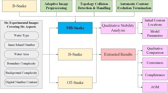
As mentioned above, the B-Snake method yields better results than other topology inflexible parametric snakes when extracting boundaries of deep concave regions and small tubular branches. It lacks topology transformation capability, and employing the ACID technique to enable the curve to split and merge, as do topology-flexible parameter snakes, generally decreases the accuracy. Is there a method that does not use the grid decomposition technique, yet enables the B-Snake method to become topology adaptive, ensuring accuracy and topology flexibility? The main contribution of this paper is to propose a modified B-Snake (MB-Snake) method based on the B-Snake method to achieve topology adaptive boundary extraction with high accuracy for irregular and complicated water bodies with multiple inner islands from satellite images of diverse land use types. Moreover, the MB-Snake method is also designed to overcome two of the intrinsic defects of the B-Snake method, including weak boundary overflow and termination of the contour evolution via fixed iteration times that are set manually instead of by the automatic judgment of the algorithm.

This paper is organized as follows. The necessary background of the B-Snake method is briefly presented in Section 2. Section 3 discusses how to avoid weak boundary overflow, perform topology collision detection and handling, and terminate the contour evolution automatically in the proposed MB-Snake method. Experimental satellite images and the corresponding extraction results are given in Section 4. Section 5 first qualitatively analyzes the extraction results and then assesses the MB-Snake, the B-Snake, and the OT-Snake methods from a quantitative view before finally discussing the stability of the MB-Snake method. Concluding remarks and outlooks are provided in Section 6.

2. B-Snake Method

The B-Snake is a parametric curve v(s) = (x(s), y(s)), where s refers to the normalized arc length, and s ∈ (0, 1) that minimizes the energy functional [27]:

$$\mathrm{E}(\mathrm{v})={\displaystyle \underset{0}{\overset{1}{\int }}\frac{1}{2}(\mathsf{\alpha }(\mathrm{s})|{\mathrm{v}}^{\prime }(\mathrm{s}){|}^2+\mathsf{\beta }(\mathrm{s})|{\mathrm{v}}^{″}(\mathrm{s}){|}^2)+}{\mathrm{k}}_1\overrightarrow{\mathrm{N}(\mathrm{s})}-\mathrm{k}\frac{\nabla \mathrm{P}}{||\nabla \mathrm{P}||}\mathrm{d}\mathrm{s}$$

(1)

where α(s)|v′(s)|² + β(s)|v″(s)|² represents the internal energy; ${\mathrm{k}}_1\overrightarrow{\mathrm{N}(\mathrm{s})}-\mathrm{k}\frac{\nabla \mathrm{P}}{||\nabla \mathrm{P}||}$ is the external energy; v′(s) and v″(s) denote the first and second derivatives of the curve with respect to sand control the smoothness and continuity of the curve, respectively; $\overrightarrow{\mathrm{N}(\mathrm{s})}$ is the unit outward normal of the contour, and it acts as the inflation force; $\nabla \mathrm{P}$ is the gradient of the external energy; $\Vert \nabla \mathrm{P}\Vert$ is the norm of $\nabla \mathrm{P}$, and $\frac{\nabla \mathrm{P}}{||\nabla \mathrm{P}||}$ is the image force; α(s) and β(s) are the coefficients of the smoothing force and the continuity force, respectively, and both are non-negative quantities; and k₁ is the coefficient of the inflation force. When k₁ > 0, the curve expands outward, otherwise, it contracts inward; k is the weight of the image force, and it is non-negative.

To obtain the minimum of E(v), according to the Euler–Lagrange equation [36], v(s) should satisfy the equation

$$(\mathsf{\alpha }(\mathrm{s}){\mathrm{v}}^{\prime }(\mathrm{s}){)}^{\prime }-(\mathsf{\beta }(\mathrm{s}){\mathrm{v}}^{\prime \prime }(\mathrm{s}){)}^{\prime \prime }-\nabla ({\mathrm{k}}_1\overrightarrow{\mathrm{N}(\mathrm{s})}-\mathrm{k}\frac{\nabla \mathrm{P}}{||\nabla \mathrm{P}||})=0$$

(2)

Using finite difference method to transform Equation (2), the iterative formula for calculating the coordinates of contour nodes can be acquired:

$${\mathrm{v}}^{\mathrm{n}}={(\mathrm{I}-\mathsf{\tau }\mathrm{A})}^{-1}({\mathrm{v}}^{\mathrm{n}-1}-\mathsf{\tau }\left(\nabla ({\mathrm{k}}_1\overrightarrow{\mathrm{N}(\mathrm{s})}-\mathrm{k}\frac{\nabla \mathrm{P}}{||\nabla \mathrm{P}||})\right)({\mathrm{v}}^{\mathrm{n}-1}))$$

(3)

where vⁿ and vⁿ⁻¹ represent the N × 2 order matrix (N is the number of discrete control points of the contour) comprising the contour node coordinates of the nth and (n − 1)th iteration, respectively; A is the N × N matrix, and

$$\mathrm{A}=\left(\begin{array}{cccccccc}\mathrm{c}& \mathrm{b}& \mathrm{a}& 0& \dots & 0& \mathrm{a}& \mathrm{b}\\ \mathrm{b}& \mathrm{c}& \mathrm{b}& \mathrm{a}& 0& \dots & 0& \mathrm{a}\\ \mathrm{a}& \mathrm{b}& \mathrm{c}& \mathrm{b}& \mathrm{a}& 0& \dots & 0\\ 0& \mathrm{a}& \mathrm{b}& \mathrm{c}& \mathrm{b}& \mathrm{a}& 0& 0\\ & & & & \dots & & & \\ 0& \dots & 0& \mathrm{a}& \mathrm{b}& \mathrm{c}& \mathrm{b}& \mathrm{a}\\ \mathrm{a}& 0& \dots & 0& \mathrm{a}& \mathrm{b}& \mathrm{c}& \mathrm{b}\\ \mathrm{b}& \mathrm{a}& 0& \dots & 0& \mathrm{a}& \mathrm{b}& \mathrm{c}\end{array}\right)$$

where a = −β(s), b = 4β(s) + α(s), c = −6β(s) − 2α(s), and I is the N order identity matrix;$\left(\nabla ({\mathrm{k}}_1\overrightarrow{\mathrm{N}(\mathrm{s})}-\mathrm{k}\frac{\nabla \mathrm{P}}{||\nabla \mathrm{P}||})\right)({\mathrm{v}}^{\mathrm{n}-1})$ is the N × 2 order matrix consisting of the x and y coordinate components of the negative gradient of the external balloon snake in all contour nodes of the (n − 1)th iteration; $\mathsf{\tau }=\frac{\mathsf{\Delta }\mathrm{t}}{\mathsf{\gamma }}$, where △t is the time interval between the nth and (n − 1)th iteration; and γ denotes the empirical coefficient.

3. Proposed MB-Snake Method

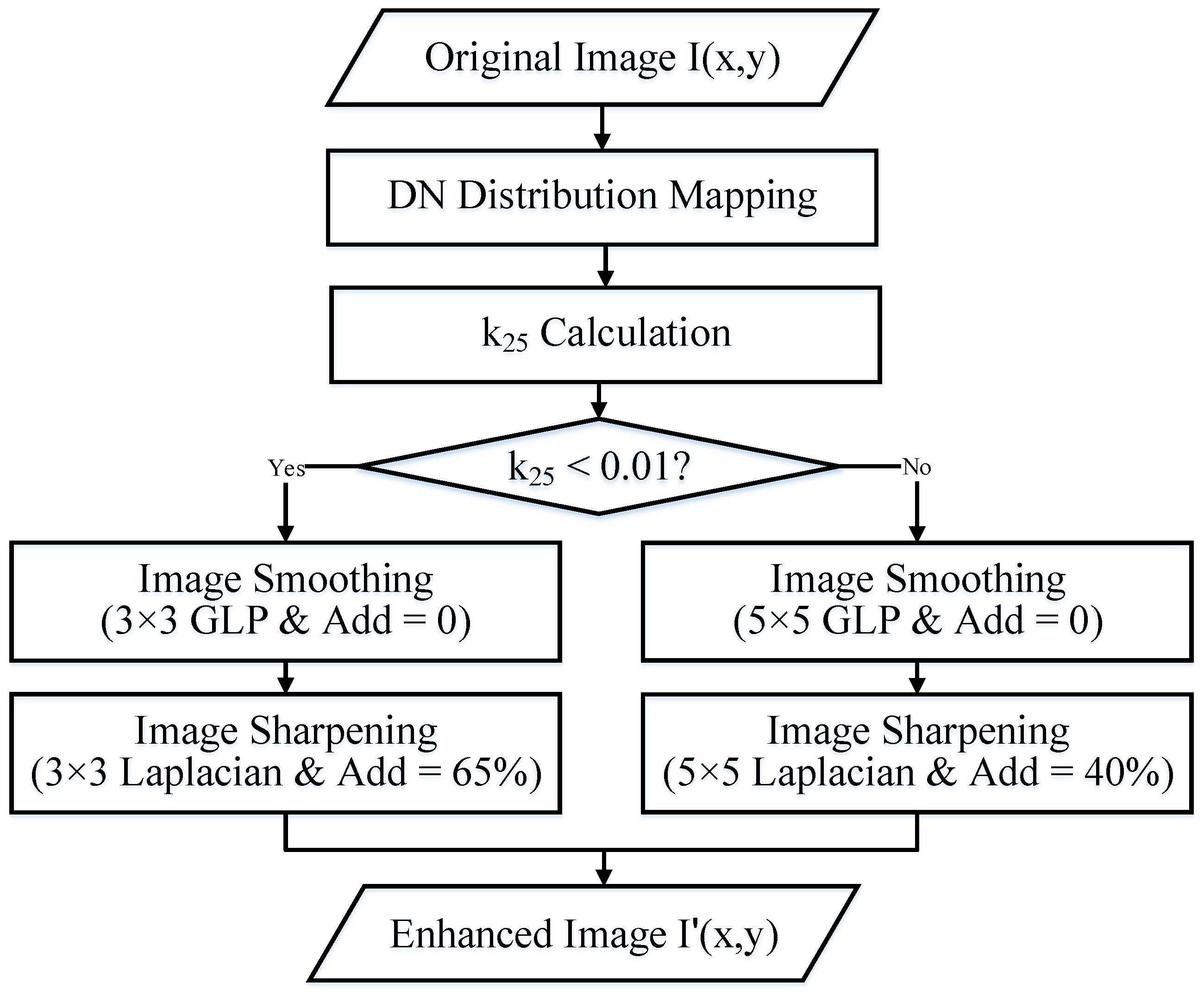
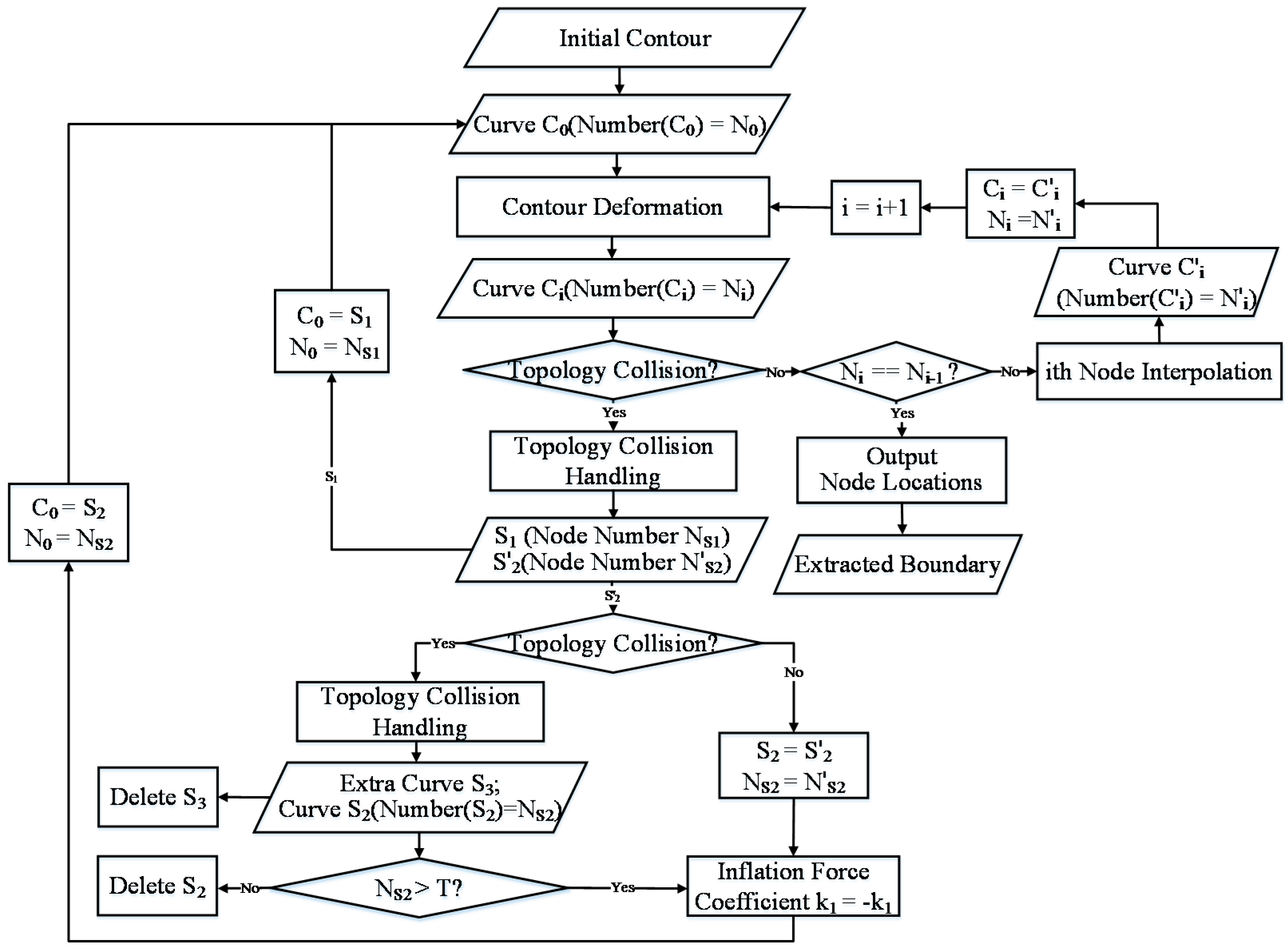
Based on the reusability of the external force expression and the energy formula of the B-Snake method, the MB-Snake method introduces three strategies to solve the abovementioned three problems. In terms of the weak boundary overflow problem when faced with images with low digital number (DN) value contrast, the MB-Snake method introduces an adaptive image preprocessing schema to perform image sharpening based on the characteristics of different DN value distribution patterns of satellite images, with images of varied DN value contrast having different preprocessing procedures. With respect to the topology collision problem, the MB-Snake method adds a topology collision detection and handling mechanism, which breaks the initial single contour line into multiple contours by interrupting and reconnecting the line, enabling the MB-Snake method to extract boundaries for objects with inner islands. As for the termination criterion for contour evolution, the MB-Snake method will be terminated when the curve node number remains unchanged during the last two iterations instead of using a fixed iteration time. The adaptive image preprocessing of the MB-Snake method is demonstrated in Figure 1. The topology collision detection, handling, and contour termination of the MB-Snake method is displayed in Figure 2.

3.1. Adaptive Image Preprocessing

Different images have varied DN value contrast, and the B-Snake method has distinct performances on images with different DN value contrast. The B-Snake method is often faced up with serious weak boundary overflows in images with low DN value contrast, resulting in inaccurate extracted boundaries. Therefore, the MB-Snake method proposed in this paper employs a self-adaptive image preprocessing strategy with different window sizes and add back values for images with different DN value contrasts to resolve this problem.

To be specific, the self-adaptive image preprocessing strategy is composed of four main steps:

(1) DN value distribution diagram generation

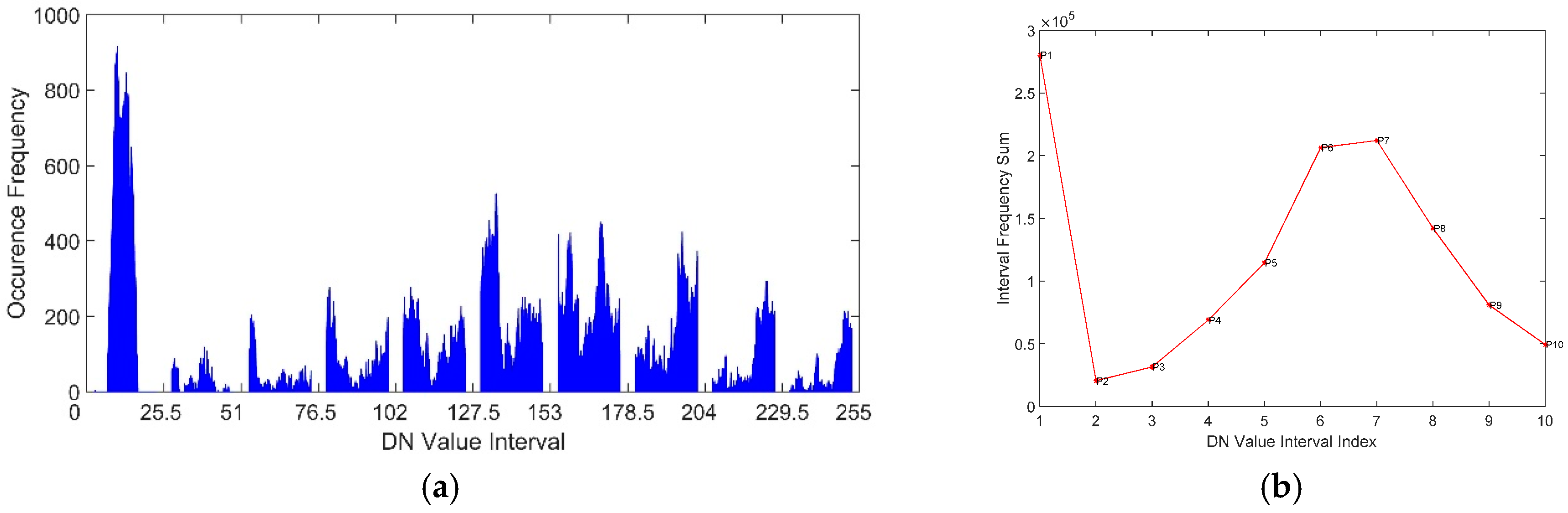
The DN value distribution diagram is generated by uniformly dividing the DN values into ten groups, and counting the number of pixels the DN value of which fall in the same value range. One of the sample DN value distribution diagram is demonstrated in Figure 3a. The number ten is an empirical value determined by multiple trials, and it could provide optimal results for DN value contrast distinguishing and judgment.

(2) DN value contrast judgment

Function y_i = f(x_i), where x_i = 1, 2,…, 10, y_i is the number of pixels the DN value of which fall in the value range of [(x_i − 1) × 255 / 10, x_i × 255 / 10) can be acquired from step (1). Here the DN value contrast is categorized into two types, including high and low, according to k₂₅, the absolute value of the slope of the straight line determined by point P₂(x₂, y₂) and point P₅(x₅, y₅). The definition of k₂₅ is displayed in Figure 3b. The reason why the points P₂ and P₅ are selected is that different types of satellite images have distinctly different k₂₅, and satellite images can be separated much more easily by using them. The images with k₂₅ > 0.01 are classified into images with low DN value contrast, otherwise are high. The threshold 0.01 is an empirical value determined by multiple trials. In fact, the values of k₂₅ are quite different for satellite images of varied DN value contrasts, thus the threshold is not that sensitive, with the values between 0.01 and 0.15 all competent for the separation.

(3) Self-adaptive image smoothing

For the images with high DN value contrast, a Gaussian Low Pass filter with the window size 3 × 3 pixels and add back value 0 is adopted to perform image smoothing, while for the images with low DN value contrast, the window size is 5 × 5 pixels and the add back value stays 0. The window sizes and add back values were empirical values determined by multiple trials, and they could help in acquiring better extraction results. The reason why the window size for the images with low DN value contrast is larger is that there is more noise in those images with low DN value contrast, and larger window size is more conducive to noise suppression. However, larger window size reduces the positioning accuracy of boundaries, so the window sizes are set 3 × 3 pixels for images with high DN value contrast and 5 × 5 pixels for images with low DN value contrast by making an balance between noise and positioning accuracy;

(4) Self-adaptive boundary enhancement

For the images with high DN value contrast, a Laplacian operator with the window size 3 × 3 pixels and add back value 65% is adopted to perform boundary enhancement, while for the images with low DN value contrast, the window size is 5 × 5 pixels and the add back value is 40%. The window sizes and add back values were empirical values determined by multiple trials, and they could help in acquiring better extraction results. The reason why the window size is set larger and the add back value is set smaller for the images with low DN value contrast is that they both could ensure better effects of border enhancement, avoiding weak boundary overflow phenomena to the maximum. Using three-step image preprocessing, strong borders are maintained and weak boundaries are enhanced to go into the next step for topology collision detection and handling.

3.2. Topology Collision Detection and Handling

3.2.1. Topology Collision Detection

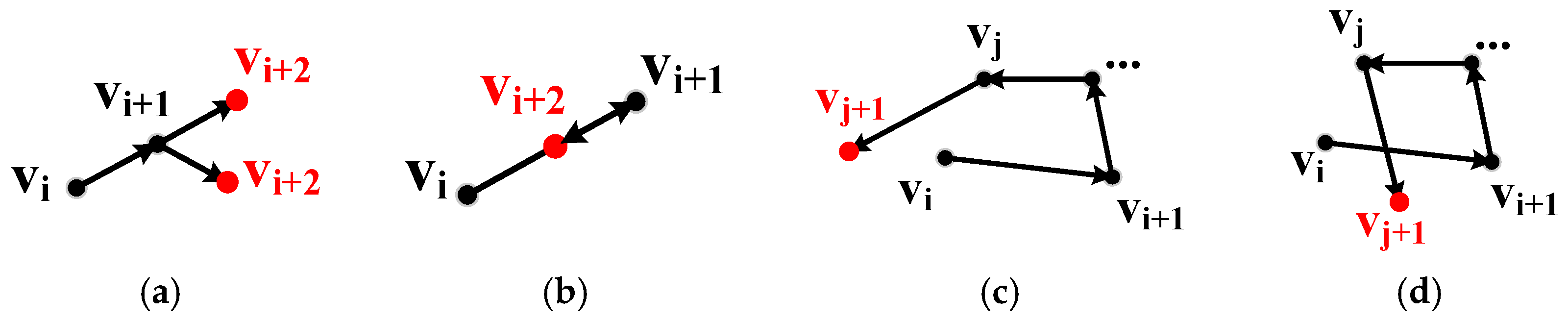
The curve without topology collisions is a series of nodes connected in sequence from head to tail, and not any two adjacent line segments are collinear and reverse, and not any non-adjacent line segments intersect with each other. Figure 4a,c shows the curves without topology collisions, Figure 4b the curve with topology collisions in adjacent line segments, and Figure 4d the curve with topology collisions in non-adjacent line segments. Topology collision detection is to determine whether the situations in Figure 4b,d occur, and at which points they occur. For the adjacent line segments shown in Figure 4a,b, assuming V_i = (x_i, y_i), V_i+1 = (x_i+1, y_i+1), V_i+2 = (x_i+2, y_i+2), if the vector $\overrightarrow{{\mathrm{V}}_{\mathrm{i}}{\mathrm{V}}_{\mathrm{i}+1}}$ and $\overrightarrow{{\mathrm{V}}_{\mathrm{i}+1}{\mathrm{V}}_{\mathrm{i}+2}}$ satisfy:

$$\overrightarrow{{\mathrm{V}}_{\mathrm{i}}{\mathrm{V}}_{\mathrm{i}+1}}\times \overrightarrow{{\mathrm{V}}_{\mathrm{i}+1}{\mathrm{V}}_{\mathrm{i}+2}}=\left({\mathrm{x}}_{\mathrm{i}+1}-{\mathrm{x}}_{\mathrm{i}}\right)*\left({\mathrm{y}}_{\mathrm{i}+2}-{\mathrm{y}}_{\mathrm{i}+1}\right)-\left({\mathrm{x}}_{\mathrm{i}+2}-{\mathrm{x}}_{\mathrm{i}+1}\right)*\left({\mathrm{y}}_{\mathrm{i}+1}-{\mathrm{y}}_{\mathrm{i}}\right)=0$$

$$\mathrm{and}\left({\mathrm{x}}_{\mathrm{i}+2}-{\mathrm{x}}_{\mathrm{i}+1}\right)=\mathsf{\lambda }\left({\mathrm{x}}_{\mathrm{i}+1}-{\mathrm{x}}_{\mathrm{i}}\right)\left(\mathsf{\lambda }<0\right)||\left({\mathrm{y}}_{\mathrm{i}+2}-{\mathrm{y}}_{\mathrm{i}+1}\right)=\mathsf{\lambda }\left({\mathrm{y}}_{\mathrm{i}+1}-{\mathrm{y}}_{\mathrm{i}}\right)\left(\mathsf{\lambda }<0\right),$$

topology collision exists in the nodes V_i, V_i+1, and V_i+2, otherwise no topology collision exists.

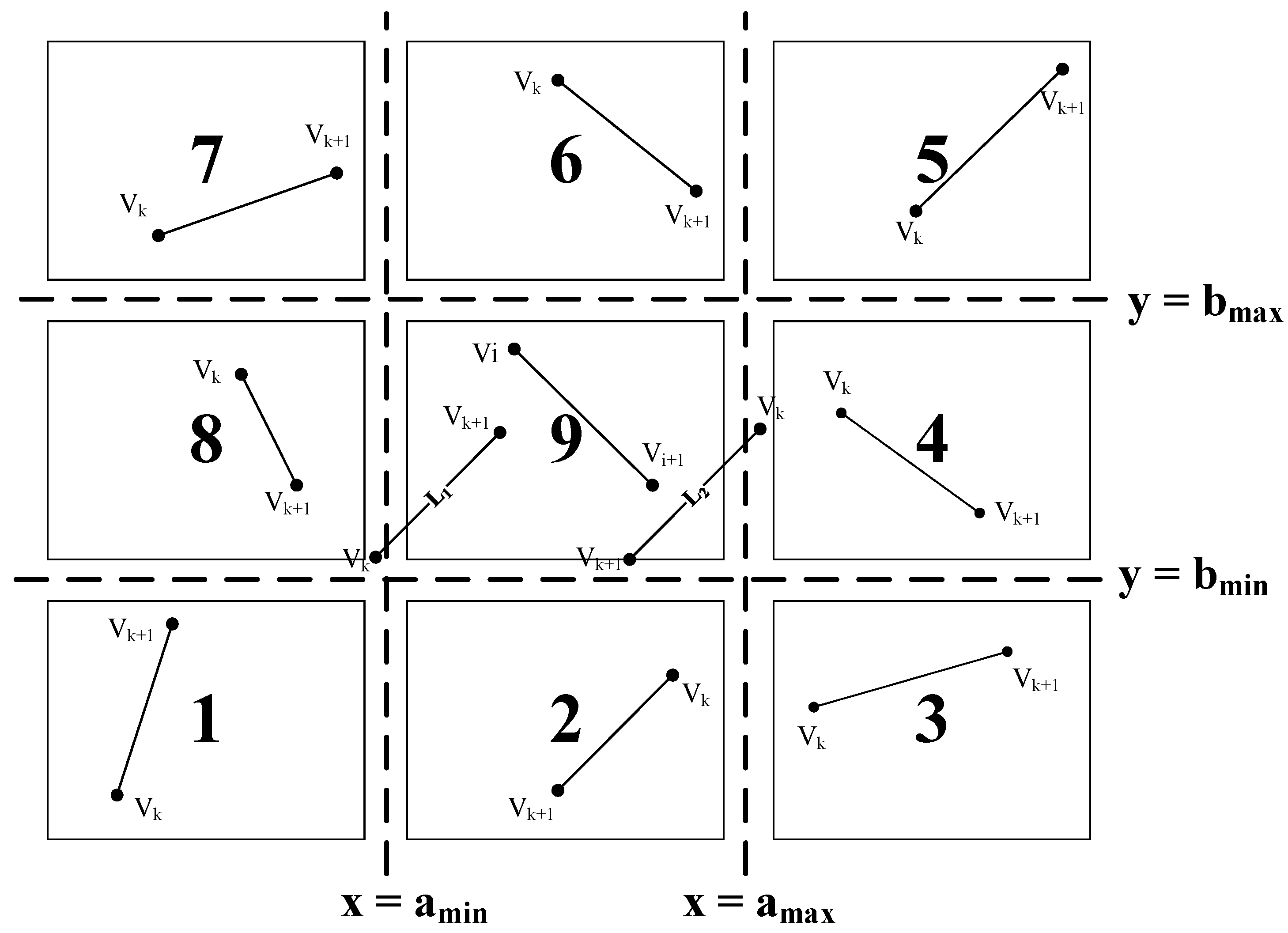
The intersection detection of non-adjacent line segments displyed in Figure 4d can be quite complicated. All the possible relative position relationships between V_iV_i+1 (i ∈ N, 1 ≤ i ≤ n−3, n is the total node number of the curve S₀), and V_kV_k+1 (k ∈ N, i+1 ≤ k ≤ n−1) are demonstrated in Figure 5. Assuming V_i = (a₁, b₁), V_i+1 = (a₂, b₂), V_k = (c₁, d₁), V_k+1 = (c₂, d₂), and a_min = min{a₁, a₂}, a_max = max{a₁, a₂}, b_min = min{b₁, b₂}, b_max = max{b₁, b₂}, c_min = min{c₁, c₂}, c_max = max{c₁, c₂}, d_min = min{d₁, d₂}, d_max = max{d₁, d₂}, the two-dimensional plane is divided into nine regions, numbered 1 to 9, by the four lines x = a_min, x = a_max, y = b_min, and y = b_max, the situations in which the line segment V_iV_i+1 will not intersect with V_kV_k+1 are listed below.

(1)

c_min > a_max, as the line segment V_kV_k+1 shown in regions 3, 4, and 5;

(2)

c_max < a_min, as the line segment V_kV_k+1 shown in regions 1, 7, and 8;

(3)

d_min > b_max, as the line segment V_kV_k+1 shown in regions 5, 6, and 7;

(4)

d_max < b_min, as the line segment V_kV_k+1 shown in regions 1, 2, and 3;

(5)

V_k and V_k+1 lie in the same side of the line determined by V_i and V_i+1, as the line segment V_kV_k+1 shown in the L₁ location of region 9; and

(6)

V_i and V_i+1 lie in the same side of the line determined by V_k and V_k+1, as the line segment V_kV_k+1 shown in the L₂ location of region 9.

When i = n, the line segment V_iV_i+1 = V_nV₁ and the line segment V_kV_k+1 = V₁V₂, and the topology collision detection conditions and processes are the same as abovementioned. If the line segments V_iV_i+1 and V_kV_k+1 satisfy one of the abovementioned six conditions, there is no topology collision in the curve, otherwise topology collision exists.

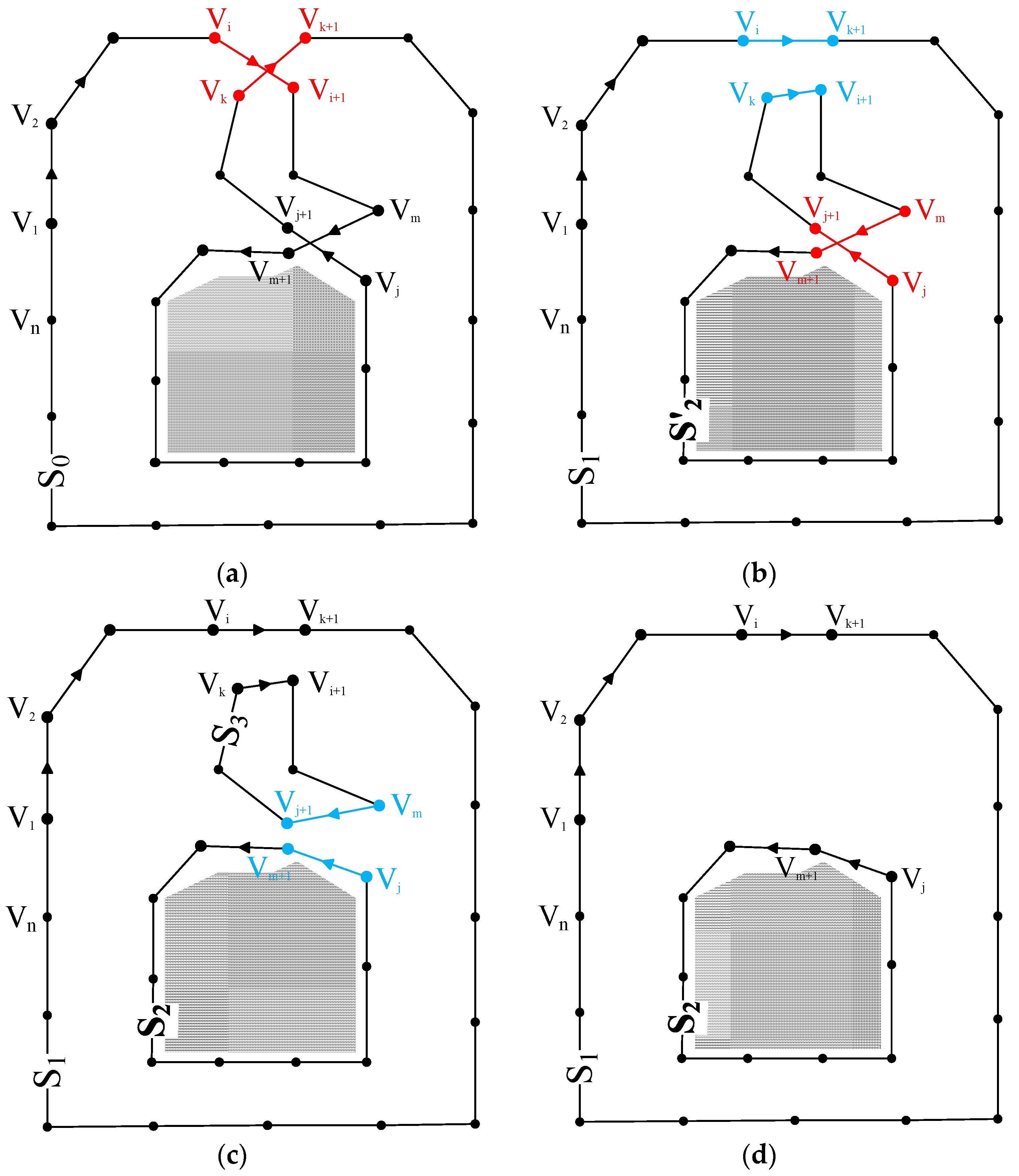
3.2.2. Topology Collision Handling

The MB-Snake method disposes of the topology collisions via successive interrupting and reconnecting of the two related pairs of line segments. Assuming all the nodes of the curve S₀ are arranged clockwise, and that the topology collision detection procedure has detected that the line segment V_iV_i+1 intersects with V_kV_k+1, and the line segment V_jV_j+1 intersects with V_mV_m+1, as the topology collision situation shown in Figure 6a, the topology collision handling of the MB-Snake method will be implemented via the following three steps:

(1) 1st Interruption and Reconnection: Disconnect the two intersecting line segments V_iV_i+1 and V_kV_k+1 and reconnect head node V_i of line segment V_iV_i+1 with tail node V_k+1 of line segment V_kV_k+1. Then, reconnect tail node V_i+1 of line segment V_iV_i+1 with head node V_k of line segment V_kV_k+1. Through the first interruption and reconnection, the curve splits into an exterior curve S₁ = {V₁, V₂, …., V_i, V_k+1, V_k+2, …, V_n} and an interior curve S′₂ = {V_i+1, V_i+2, …, V_k}. However, as demonstrated in Figure 6b, self-intersection still exists for S′₂.

(2) Second Interruption and Reconnection: Repeat Step (1) to split curve S′₂ into a new curve S₂ = {V_m+1, V_m+2, …, V_j}, without self-intersections, and an extra closed loop S₃ = {V_i+1, V_i+2, …, V_m, V_j+1, V_j+2, …, V_k}, as displayed in Figure 6c.

(3) Extra Curve Deletion: Curve S₂ may be speckle noise or true islands, but given that the node number of speckle noise is usually much smaller than that of true islands, whether curve S₂ is kept depends on whether the node number of it is larger than the threshold in this paper. Counting the node number of S₂ and recording it as N, if N < T (T is the empirical threshold of the node number of speckle noise, and T = 50 via multiple trials), curve S₂ will be viewed as speckle noise and deleted; otherwise, it will be kept. Curve S₃ is an extra curve produced during topology collision processing. It is deleted, as shown in Figure 6d.

Through the abovementioned topology collision detection and handling mechanism, the original curve S₀ can be split into exterior curve S₁ and interior contour S₂, and topology collisions existing in the water images with islands can be managed. Then, continuing the iterative evolution of curve S₁, setting k₁ = −k₁, and continuing the evolution of curve S₂, the correct object boundaries can be finally acquired. If there are p islands in an image, this topology collision detection and handling mechanism will be repeated p times to address all the topology collisions.

3.3. Definite Termination of Contour Evolution

Present termination criteria of contour evolution do not incorporate contour change information effectively, and termination of contour evolution is implemented manually based on a predefined number of iterations. However, the possible number of iterations required cannot be easily determined in advance. Correspondingly, fewer iterations will lead to incomplete contours, while more iterations will consume unnecessary time and waste computational resources. The MB-Snake method proposed in this paper attempts to automatically terminate contour evolution by monitoring the contour node number changes between two adjacent iterations. When the contour node number remains unchanged from the ith iteration to the (i + 1)th iteration, contour deformation will stop. The contour acquired at this time is the true boundary of the target.

4. Experiments and Results

This section presents extraction experiments using the MB-Snake method. For comparison, the corresponding results of the original B-Snake and the topology flexible OT-Snake method are also provided. The experiments were implemented using Matlab on a normally configured computer with Inter(R) Core(TM) i3-2100 CPU @ 3.10 GHz and 8.00 GB RAM.

4.1. Experimental Data

Satellite images with water bodies were used to verify the feasibility of the MB-Snake method proposed in this paper. Although there are many types of water, including lakes, rivers, ponds, reservoirs, etc., their features can all be represented by lakes and rivers, with lakes often having complicated boundaries and usually being able to be completely contained in a single satellite image and rivers often having relatively simple borders and in most cases extending too much to be completely contained in a single satellite image, and water can also be partitioned into three categories based on the number of islands, with zero, one, or multiple islands. The experimental data selected here covered six types, including lakes or rivers with zero, one, or multiple islands. The six satellite images used are from the near-infrared (NIR) bands (spectral range: 0.77–0.89 μm) of the images acquired by the wide field of view (WFV) sensor on the GF-1 satellite, with a spatial resolution of 16 m. The GF-1 satellite is sun-synchronous, with the orbit height of 645 km, and the orbit inclination of 98.0506°. Two 2-m panchromatic/8-m multi-spectral cameras with the image width of 60 km and the revisiting period of four days, and four 16-m multi-spectral cameras with the image width of 800 km and the revisiting period of two days, were equipped with the GF-1 satellite. The reason why the NIR band is selected is that water is strongly absorbed in the near infrared band, and thus water bodies have more clear boundaries in the NIR band images.

As displayed in Figure 7, the six GF-1 satellite experimental images used in this paper covered images of different water types, inner island number, sizes, boundary and background complexities, and DN value contrasts. In terms of boundary complexity, if there are many deep concaves, small tubular branches, or multiple inner islands in the water body boundaries of an image, this image will be categorized as with high boundary complexity. When compared with rivers, there are often more deep concaves and small tubular branches in lakes, so in our submission, lakes are thought of as with high boundary complexity, while rivers are of low boundary complexity. As for background complexity, if there is more than three object types in the background, it is regarded as of high background complexity. In our submission, there are buildings, roads, water, and vegetation in the background of Figure 7f, so it is identified as with high background complexity, while there are only one or two object type(s) in other five images, they are thus categorized as with low background complexity. The high or low DN value contrast is determined by the value k₂₅, those with k₂₅ < 0.01 are images with high DN value contrast, otherwise are images with low DN value contrast.

Figure 7a is the image of the lake without an island, with 220 × 299 pixels, high boundary complexity, low background complexity, and low DN value contrast. Figure 7b is the image of the lake with a single island, with 291 × 299 pixels, high boundary complexity, low background complexity, and high DN value contrast. Figure 7c is the image of the lake with multiple islands, with 994 × 1215 pixels, high boundary complexity, low background complexity, and low DN value contrast. Figure 7d is the image of the river without an island, with 367 × 273 pixels, low boundary complexity, low background complexity, and low DN value contrast. Figure 7e is the image of the river with a single island, with 293 × 235 pixels, low boundary complexity, low background complexity, and low DN value contrast. Figure 7f is the image of the river with multiple islands, with 369 × 414 pixels, low boundary complexity, high background complexity, and low DN value contrast.

Table 1. Summary of the six GF-1 WFV experimental images. GL: geo-location; AD: acquisition date; IS: image size (units: pixels); WT: water type; IIN: inner island number; BDCP: boundary complexity; BGCP: background complexity; BDCL: boundary clarity.

Image	GL	AD	IS	WT	IIN	BDCP	BGCP	BDCL
Figure 4a	Xiaogan, Hubei	8 October 2014	220 × 299	Lake	0	High	Low	Low
Figure 4b	Xuancheng, Anhui	6 August 2015	291 × 299	Lake	1	High	Low	High
Figure 4c	Arli, Tibet	13 October 2015	994 × 1215	Lake	N	High	Low	Low
Figure 4d	Chongqing	21 October 2015	367 × 273	River	0	Low	Low	Low
Figure 4e	Chongqing	21 October 2015	293 × 235	River	1	Low	Low	Low
Figure 4f	Maanshan, Anhui	3 December 2015	369 × 414	River	N	Low	High	Low

is the summary of the characteristics of the six GF-1 WFV experimental images.

4.2. Extraction Results

The proposed MB-Snake method was applied in the aforementioned six GF-1 WFV satellite images. The B-Snake and OT-Snake methods were also used for comparison. All the results of the MB-Snake method from the six experimental images were acquired under the same set of model parameters, with α = 0.05, β = 0.0, k₁ = 0.2, and k = 2.0. Figure 8b,e,h,k,n,q shows the MB-Snake method extraction results based on Figure 7a–f, respectively. The yellow circles in these figures are the initial contours, and the red boundaries are the borders acquired by the MB-Snake method.

In terms of the B-Snake method, its iteration times for the six images were estimated based on the memory requirements and time consumption under the fact that the B-Snake contour could not be able to split and the B-Snake deformation cannot stop automatically, which means that more iteration times will produce more complicated curves, demanding high requirements for computer memory and consuming plenty of time. The iteration times of the B-Snake method were set at 350, 500, 4500, 500, 500, and 900 for Figure 7a–f, respectively. The corresponding extraction results of the B-Snake method are displayed in Figure 8a,d,g,j,n,p, with the yellow circles representing initial contours identical to those of the MB-Snake method, and the red boundaries being the final extraction results.

With respect to the OT-Snake method, the extracted results were obtained under different sets of model parameters because of model parameter instabilities [35]. Figure 8c,f,i,l,o,r provides the results obtained by the OT-Snake method, in which the yellow points are the initial contours, and the red boundaries are the final extracted borders. The initial contours of the OT-Snake method were different from those of the MB-Snake and the B-Snake methods because the OT-Snake method limits its initial contour shape into a grid with four vertexes pointing into up, down, left and right, separately. Figure 8c was acquired under the set of model parameters with q = 36, λ = 2.28, ε = 1.0 × 10⁻⁷, and r = 1. The parameters were q = 38, λ = 2.28, ε = 1.0 × 10⁻⁷, and r = 1 in Figure 8f; q = 20, λ = 1, ε = 1.0 × 10⁻², and r = 1 in Figure 8i; q = 27, λ = 2.28, ε = 1.0 × 10⁻⁷, and r = 1 in Figure 8l; q = 21, λ = 2.28, ε = 1.0 × 10⁻⁷, and r = 1 in Figure 8o; and q = 30, λ = 3, ε = 1.0 × 10⁻⁷, and r = 1 in Figure 8r.

5. Performance Measure

Three evaluation indicators, including correctness [37,38,39,40], completeness [37,38,39,40], and area overlap measure (AOM) [41,42,43,44,45], are adopted in this paper to quantitatively assess the accuracy of the algorithm-extracted boundaries. Among them, correctness is to assess the boundary positioning accuracy from the aspect of polyline feature; completeness focuses on evaluating the completeness of extracted boundaries as a linear feature; and AOM is the rough estimate of the accuracy as a whole from the perspective of the polygon feature by calculating the percentage of the area that is correctly extracted. Correctness, completeness, and AOM, reflect the accuracy of the algorithm-extracted boundaries from different sides and they could be collaboratively applied in quantitative performance measure of the B-Snake, the AB-Snake, and the OT-Snake methods.

5.1. Correctness

Correctness refers to the percentage of the acquired boundaries that are correctly extracted, and it can be used to accurately evaluate the positioning accuracy of the extracted boundaries from the perspective of polyline feature. It can be obtained by calculating the length proportions of true positive (TP) boundaries, accounting for the total extracted boundaries, as depicted in Equation (4) [37,38,39,40]. TP boundaries refer to the extracted boundary segments lying within the buffer zone of the reference boundaries, as shown in Figure 9.

$$\mathrm{C}\mathrm{o}\mathrm{r}\mathrm{r}\mathrm{e}\mathrm{c}\mathrm{t}\mathrm{n}\mathrm{e}\mathrm{s}\mathrm{s}=\frac{\mathrm{L}\mathrm{e}\mathrm{n}\mathrm{g}\mathrm{t}\mathrm{h}\left\{\mathrm{T}\mathrm{P}\right\}}{\mathrm{L}\mathrm{e}\mathrm{n}\mathrm{g}\mathrm{t}\mathrm{h}\{\mathrm{T}\mathrm{P}+\mathrm{F}\mathrm{P}\}}\times 100\%$$

(4)

5.2. Completeness

Completeness refers to the percentage of the extracted boundaries that mimics the true boundaries, and it can be used to assess the integrity level of the extracted borders accurately from the aspect of polyline feature. It can be acquired by computing the lengths of true negative (TN) boundaries based on the reference boundaries, as described in Equation (5) [37,38,39,40]. TN boundaries refer to the reference boundary segments lying within the buffer zones of the extracted boundaries, as shown in Figure 10.

$$\mathrm{C}\mathrm{o}\mathrm{m}\mathrm{p}\mathrm{l}\mathrm{e}\mathrm{t}\mathrm{e}\mathrm{n}\mathrm{e}\mathrm{s}\mathrm{s}=\frac{\mathrm{L}\mathrm{e}\mathrm{n}\mathrm{g}\mathrm{t}\mathrm{h}\left\{\mathrm{T}\mathrm{N}\right\}}{\mathrm{L}\mathrm{e}\mathrm{n}\mathrm{g}\mathrm{t}\mathrm{h}\{\mathrm{T}\mathrm{N}+\mathrm{F}\mathrm{N}\}}\times 100\%$$

(5)

5.3. AOM

AOM refers to the percentage of the extracted area that takes up the overall area, and it is a quantitative evaluation indicator of the correctly extracted area, which roughly estimates the accuracy of the algorithm-extracted boundaries as a whole from the aspect of polygon features. It can be obtained by calculating the percentage that the intersection of the two regions enclosed by the algorithm-extracted boundaries and the reference boundaries takes up the union of those two regions. The formula used to compute AOM is shown in Equation (6) [41,42,43,44,45]:

$$\mathrm{A}\mathrm{O}\mathrm{M}({\mathrm{R}}_1,{\mathrm{R}}_2)=\frac{\mathrm{A}\mathrm{r}\mathrm{e}\mathrm{a}\{{\mathrm{R}}_1\cap {\mathrm{R}}_2\}}{\mathrm{A}\mathrm{r}\mathrm{e}\mathrm{a}\{{\mathrm{R}}_1\cup {\mathrm{R}}_2\}}\times 100\%$$

(6)

where R₁ and R₂ refer to the regions enclosed by the algorithm-extracted boundaries and the reference boundaries, respectively. R₁ ∩ R₂ represents the region contained in both R₁ and R₂, and R₁ ∪ R₂ refers to the region contained in either R₁ or R₂.

6. Discussion

This section first performs a qualitative analysis of the results in Figure 8a–r, then employs the three performance measures in Section 5 to perform quantitative reliability evaluations of the B-Snake, the MB-Snake, and the OT-Snake methods, and finally assesses the stability of the proposed MB-Snake method from the three aspects of initial contour locations, model parameter settings, and spatial resolutions of satellite images.

6.1. Analysis of Results

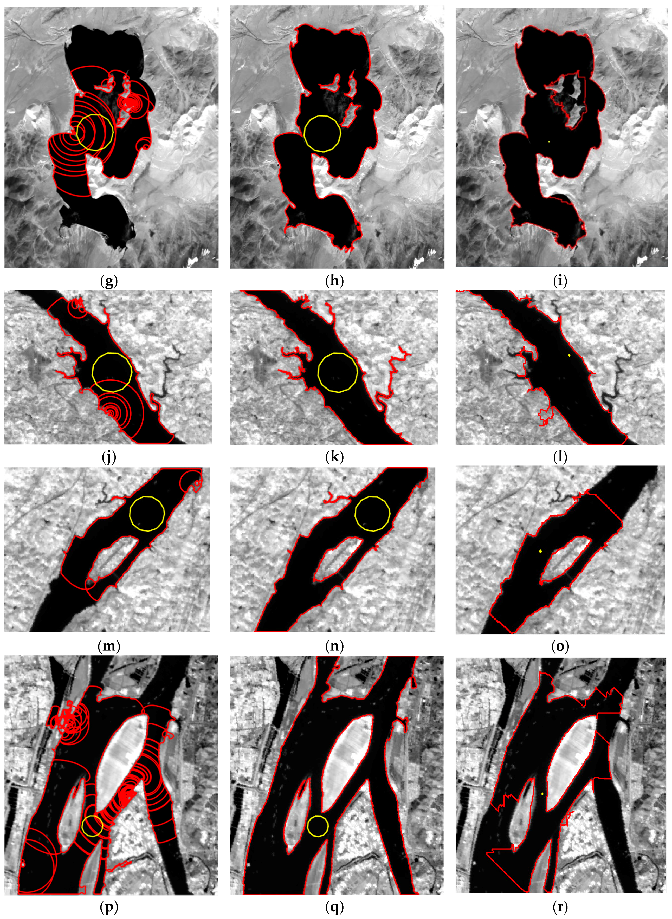
This subsection mainly discusses the differences in Figure 8a–r and qualitatively analyzes the reasons why the results are varied. It is elaborated from the two aspects of comparing the MB-Snake method proposed in this paper with the B-Snake method, which is the basis of the MB-Snake method, and the OT-Snake method, which is a newer representative of parametric snakes with topology flexibility.

6.1.1. Comparison with the B-Snake Method

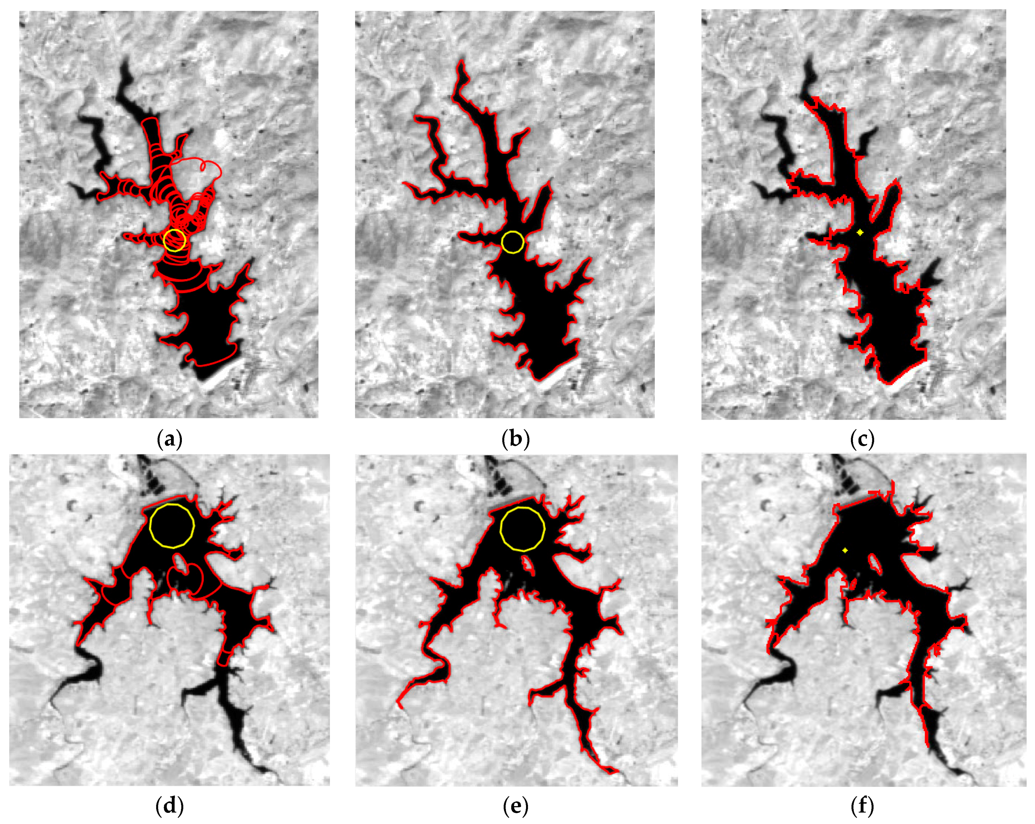
With respect to the problem of inaccurate positioning caused by weak boundary overflows, the bumps in the B-Snake-extracted results displayed in Figure 8a,g,j,p and the corresponding flat MB-Snake method borders shown in Figure 8b,h,n,q indicate that the MB-Snake method proposed in this paper is able to effectively prevent boundary overflow and improve the positioning accuracy. In terms of topology collision detection and handling, the extra boundaries inside the experimental objects in Figure 8a,d,g,j,m,p, and the correct boundaries without redundancy in Figure 8b,e,h,k,n,q suggest that the MB-Snake method possesses the capability of topology transformation. As far as automatic contour evolution termination is concerned, for the MB-Snake method, all the extraction processes used in the six experimental images were automatically terminated by determining whether the next two iterations had the same node number. For the B-Snake method, the extracted results were not stable but changed with the iteration times. The extracted borders became quite complicated and crash or memory overflow phenomena often occurred during the experimental process as the iteration times increased. Thus, the MB-Snake method achieved its design objectives improved positioning accuracy by avoiding weak boundary overflow, enabling topology collision detection and handling, and performing automatic contour evolution termination.

6.1.2. Comparison with the OT-Snake Method

In comparison with the OT-Snake method, on the one hand, as displayed in Figure 8b,e,h,n,q, the MB-Snake method could easily obtained the complete boundaries for all six experimental images, while none of the OT-Snake method extracted results could completely cover the true object boundaries; on the other hand, the MB-Snake method is parameter stable, with the same set of model parameters applicable for all six experimental images, nevertheless, as mentioned in the experiment section, despite the fact that they were the best results after trying 30 sets of parameters, not any of the six OT-Snake method results were acquired under the same set of parameters. Thus, the MB-Snake method has distinct advantages over the existing topology-flexible parametric snakes.

6.2. Reliability Evaluation

Reliability evaluation is used to check the accuracy levels of the extracted boundaries based on the three quantitative performance measures defined in Section 5, and it is implemented by comparing the extraction results with the reference boundaries, which are the comprehensive results of the boundaries acquired via manual digitalization from images with higher spatial resolution by three professionals familiar with the studied water bodies independently (the reference boundaries mentioned hereinafter are all the same). The reason why quantitative reliability evaluation was performed is that the MB-Snake extracted boundaries and the reference boundaries overlap too much to be intuitively distinguished and evaluated from the comparison figures.

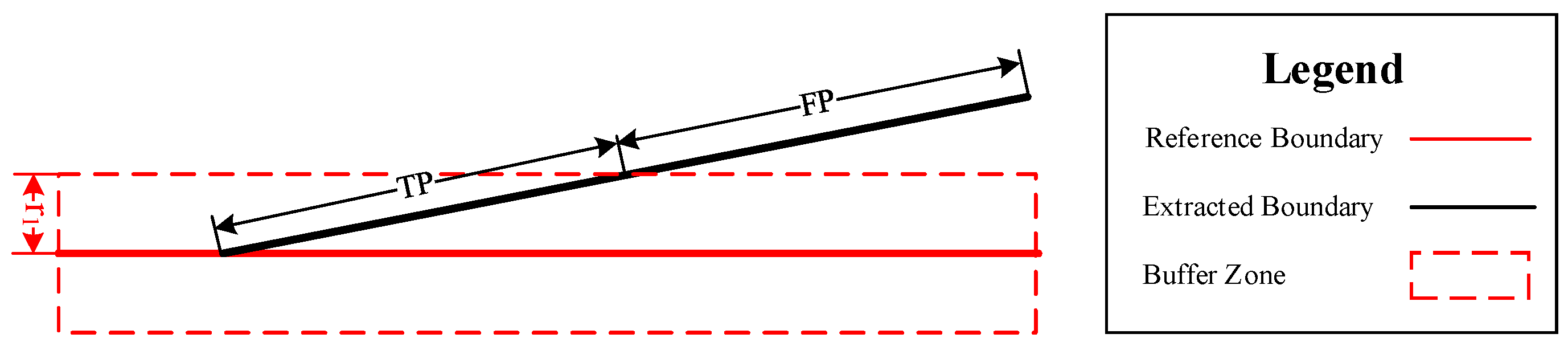
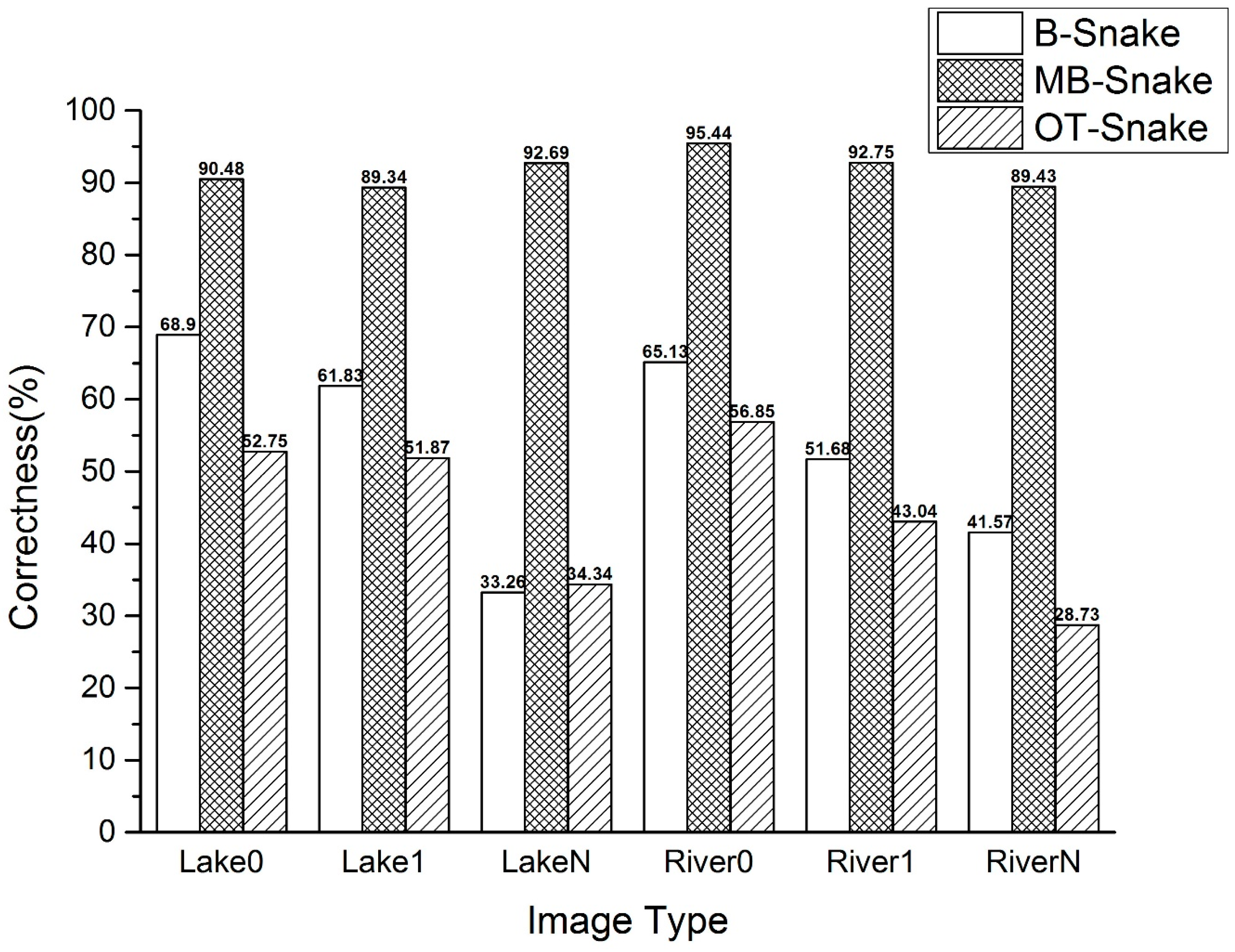
6.2.1. Positioning Accuracy

Positioning accuracy of the extracted results is evaluated based on correctness. In this paper, the buffer zone radium r₁ of the reference boundary was set as one pixel, and the correctness comparison of the B-Snake, the MB-Snake, and the OT-Snake method results using the six experimental images are shown in Figure 11. Generally, Figure 11 shows that the MB-Snake method proposed in this paper has higher positioning accuracy when compared with the accuracies of the B-Snake and OT-Snake methods. Specifically, in comparison with the B-Snake method, the MB-Snake method improves the extracted results and positioning accuracy, on one hand, by enhancing the boundary and avoiding weak boundary overflows, and on the other hand, by avoiding redundant boundary lines via the topology collision detection and handling mechanism. When compared to the OT-Snake method, the MB-Snake method exhibits distinctly higher positioning accuracies for all the six satellite images in spite of the fact that all six MB-Snake method results are acquired under the same set of model parameters, while none of the six OT-Snake method results are obtained with the same set of parameters and all the OT-Snake method results are the best results obtained by trying 30 sets of parameters. The correctness of the OT-Snake method is also lower than that of the B-Snake method, and the reason accounting for which is the OT-Snake method could not be able to extract shapes smaller than the grid size under the constraints of curve node locations.

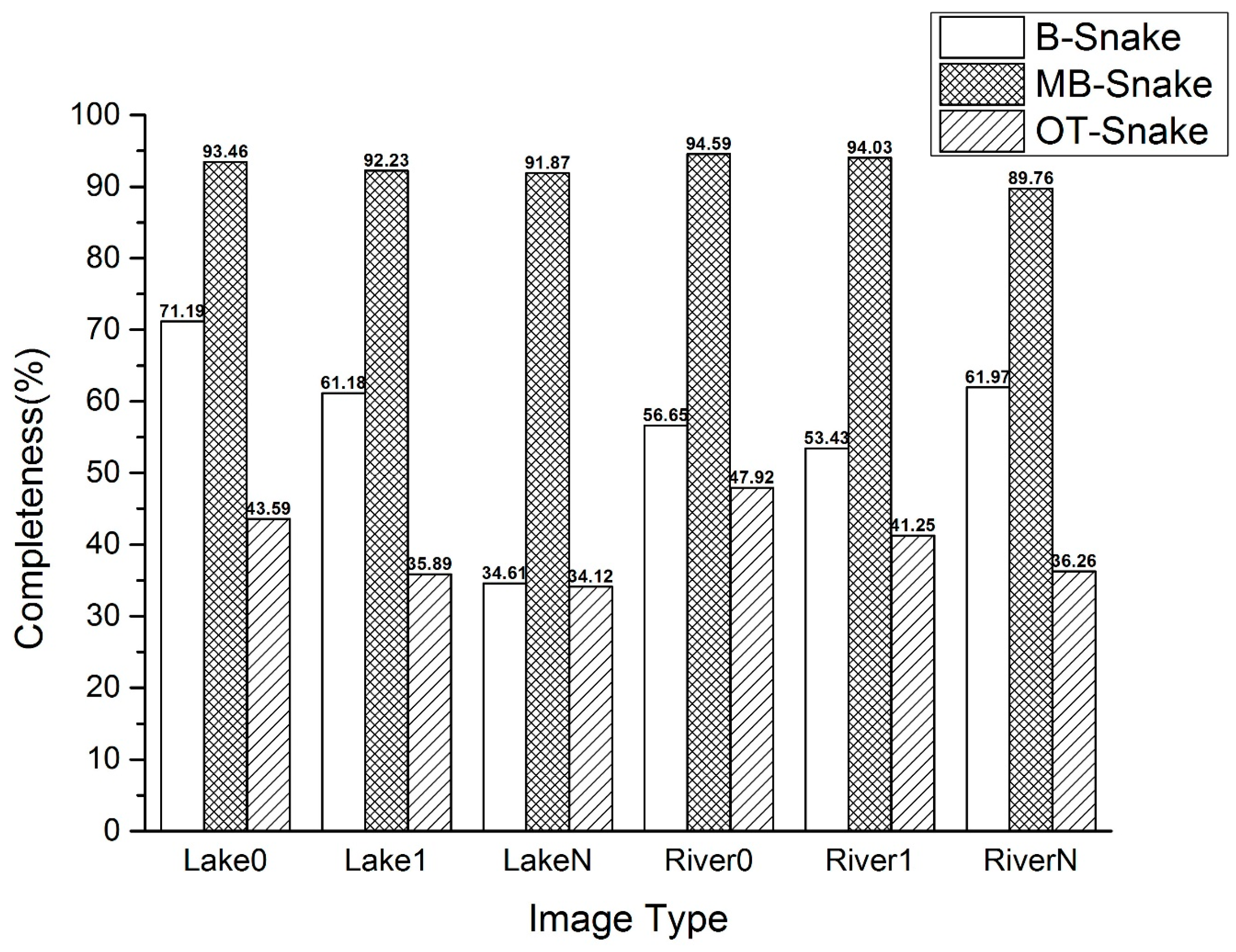
6.2.2. Integrity Level

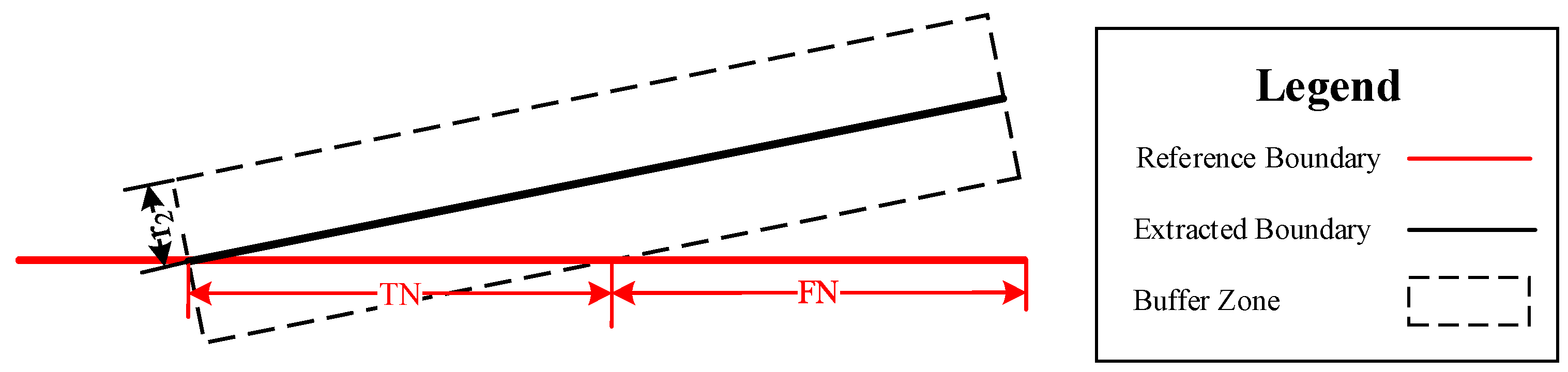
Integrity level of the extracted results is evaluated based on completeness. In this paper, the buffer zone radium r₂ of the extracted boundary was set as one pixel, and the completeness comparison of the B-Snake, the MB-Snake, and the OT-Snake method results for the six experimental images are shown in Figure 12. Generally, Figure 12 shows that the MB-Snake method proposed in this paper has a higher integrity level when compared to those of the B-Snake and OT-Snake methods. Specifically, the severe weak boundary overflows in the B-Snake method results reduced its integrity when compared with the MB-Snake method. However, compared with its correctness, the B-Snake method has higher completeness because that the redundant boundaries expanded the areas of buffer regions, and made TN larger. Despite the fact that the OT-Snake method results are the best results obtained by trying 30 sets of parameters, the completeness of the OT-Snake method is still low because the limitation of curve node locations.

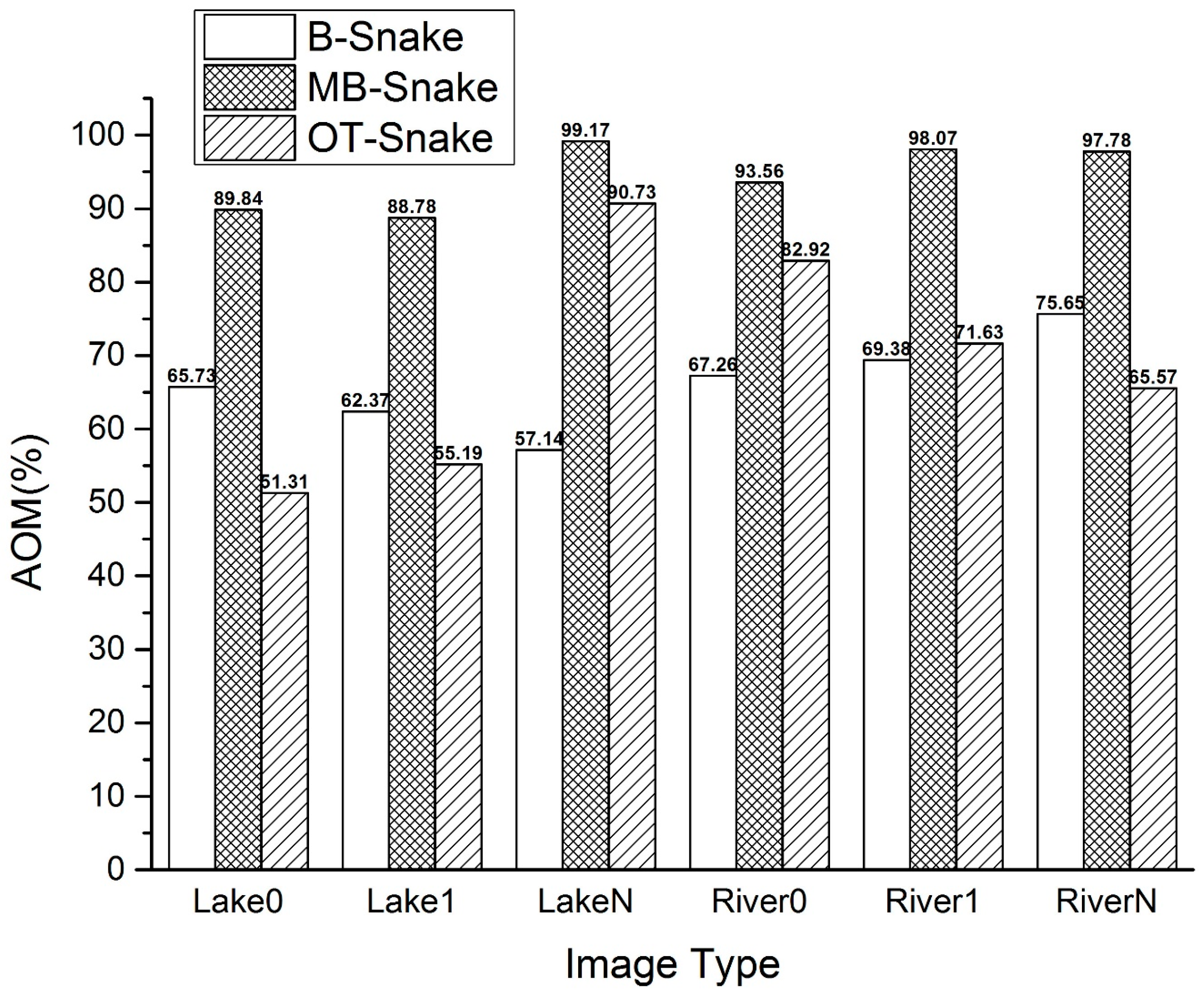
6.2.3. Overall Accuracy

Overall accuracy of the extraction results is assessed based on AOM. The AOM comparison of the B-Snake, the MB-Snake, and OT-Snake method results for the six experimental images are shown in Figure 13. Generally, the MB-Snake method has a higher AOM when compared to those of the B-Snake and OT-Snake methods. The iteration times influences the AOM of the B-Snake method, and as mentioned above, the iteration times of the B-Snake method in this paper is set under the affordable burden of computer resources and tolerable time consumption. Thus, the AOM provided here are the best values under the current experimental environment. The AOM of the OT-Snake method performs better than its correctness and completeness because of that the AOM index only cares the area of the overlap areas and does not take the positioning accuracy into consideration.

6.3. Stability Assessment

A stability assessment is used to test the stability of the MB-Snake algorithm proposed in this paper, and it is analyzed to explore the effects of initial contours and model parameters on the extracted results. The evaluation is implemented by trying different locations of initial contours and multiple pairs of model parameter values and comparatively analyzing their corresponding extracted contours to determine whether the MB-Snake method extracted results are sensitive to the locations of initial contours and how the parameters of the energy formulation affect the MB-Snake method results.

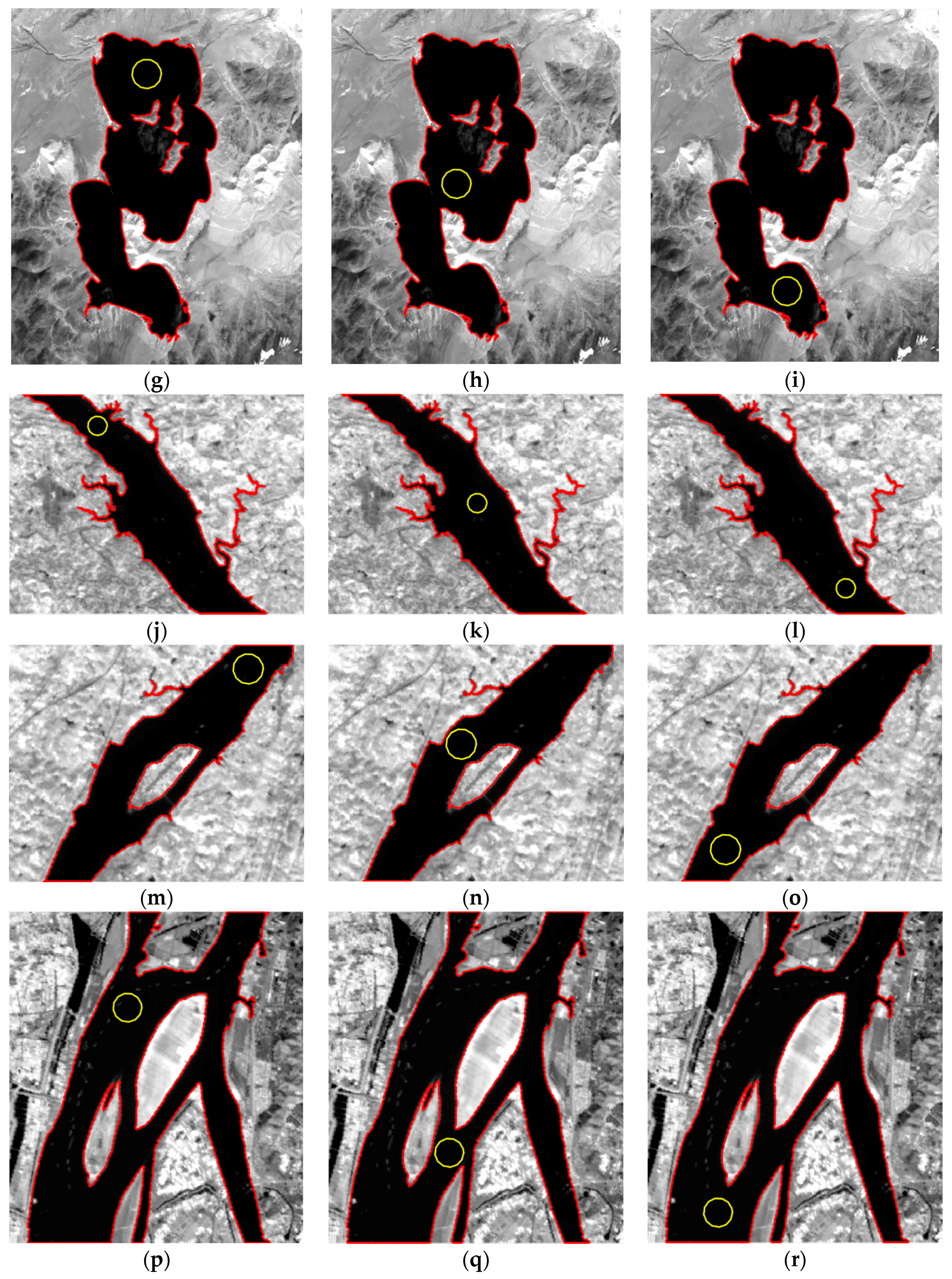
6.3.1. Sensitivity to Initial Contours

This section assesses the stability of the MB-Snake method by testing whether the MB-Snake-extracted boundaries will change with the locations of the initial contours. All six satellite images were tested with three initial contours of the same size placed in different locations of the images. During the initial contour sensitivity tests for all the six experimental images, all the model parameters were set the same, with α = 0.05, β = 0.0, k₁ = 0.2, and k = 2.0, and the corresponding extracted results were shown in Figure 14a–r, respectively. The results suggest that when the locations of the initial contours are different and other settings are the same, the extracted results remain unchanged, i.e., the MB-Snake method proposed in this paper is insensitive to the locations of initial contours.

6.3.2. Effects of Model Parameters

The effects of the four parameters α, β, k₁, and k in the energy function of the MB-Snake method are the same as those of the B-Snake method: (1) the coefficient of the first derivative α controls the smoothness of the curve; (2) the weight of the second derivative β affects the continuity of the curve; (3) the coefficient of the inflation force k₁ only influences the time consumption of the algorithm when the image force is large enough to balance the inflation force, further impacting the extracted results, resulting in boundary overflow when the image force is too small; and (4) the weight of the image force k determines whether the curve can exactly stop at true boundaries. The model parameters used in the experiment are α = 0.05, β = 0.0, k₁ = 0.2, and k = 2.0. This optimal parameter set was acquired, respectively, by keeping three of the parameters staying the same while changing the fourth one at a time, until the correctness of the extraction results achieve steady and optimal. Fifty GF-1 WFV satellite images containing water bodies of different types, inner land numbers, areas, boundary and background complexities, and digital number value contrasts were tested under this set of model parameters, and all the object boundaries were successfully extracted, demonstrating that the MB-Snake algorithm proposed in this paper is stable for model parameters.

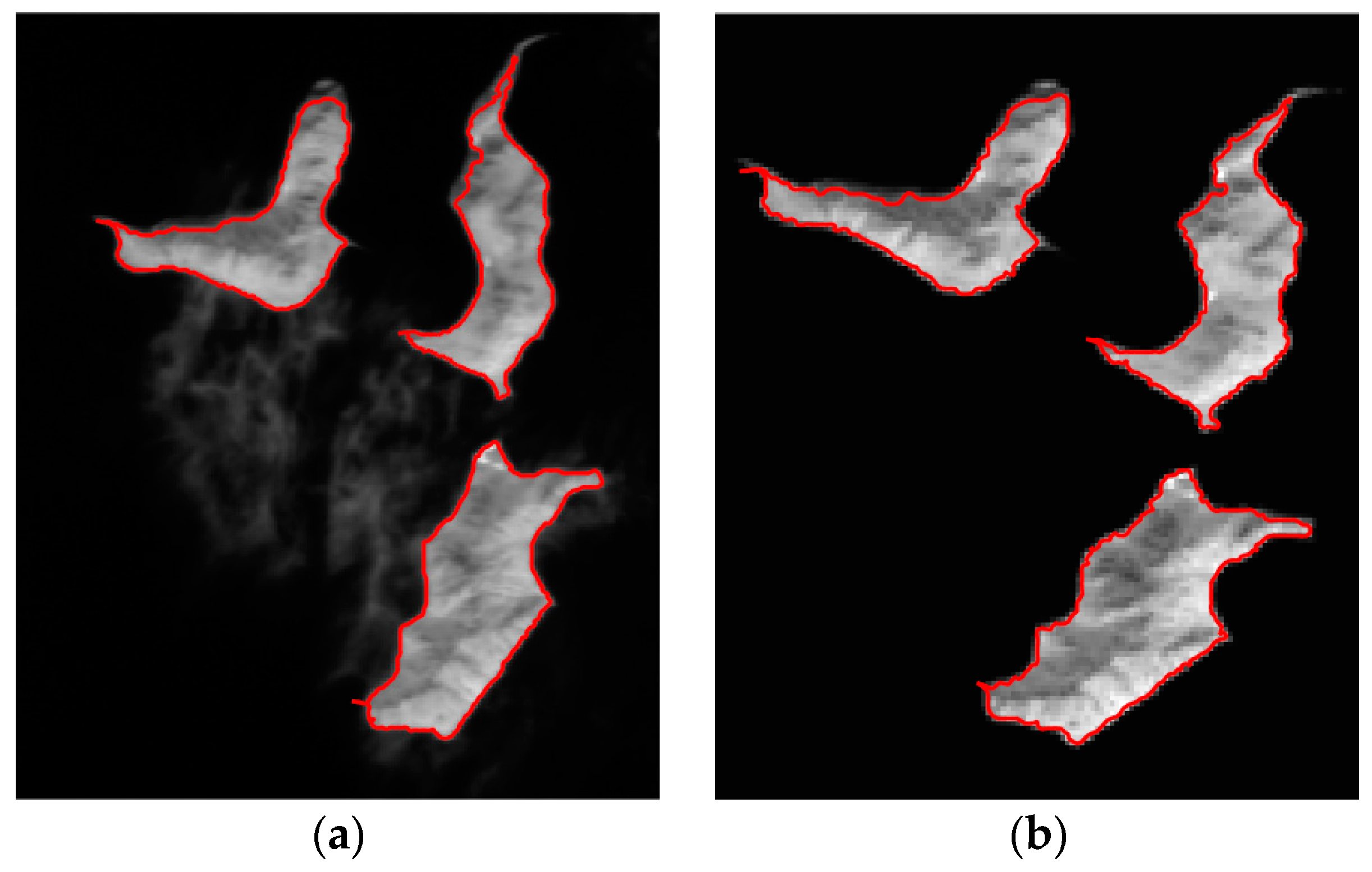
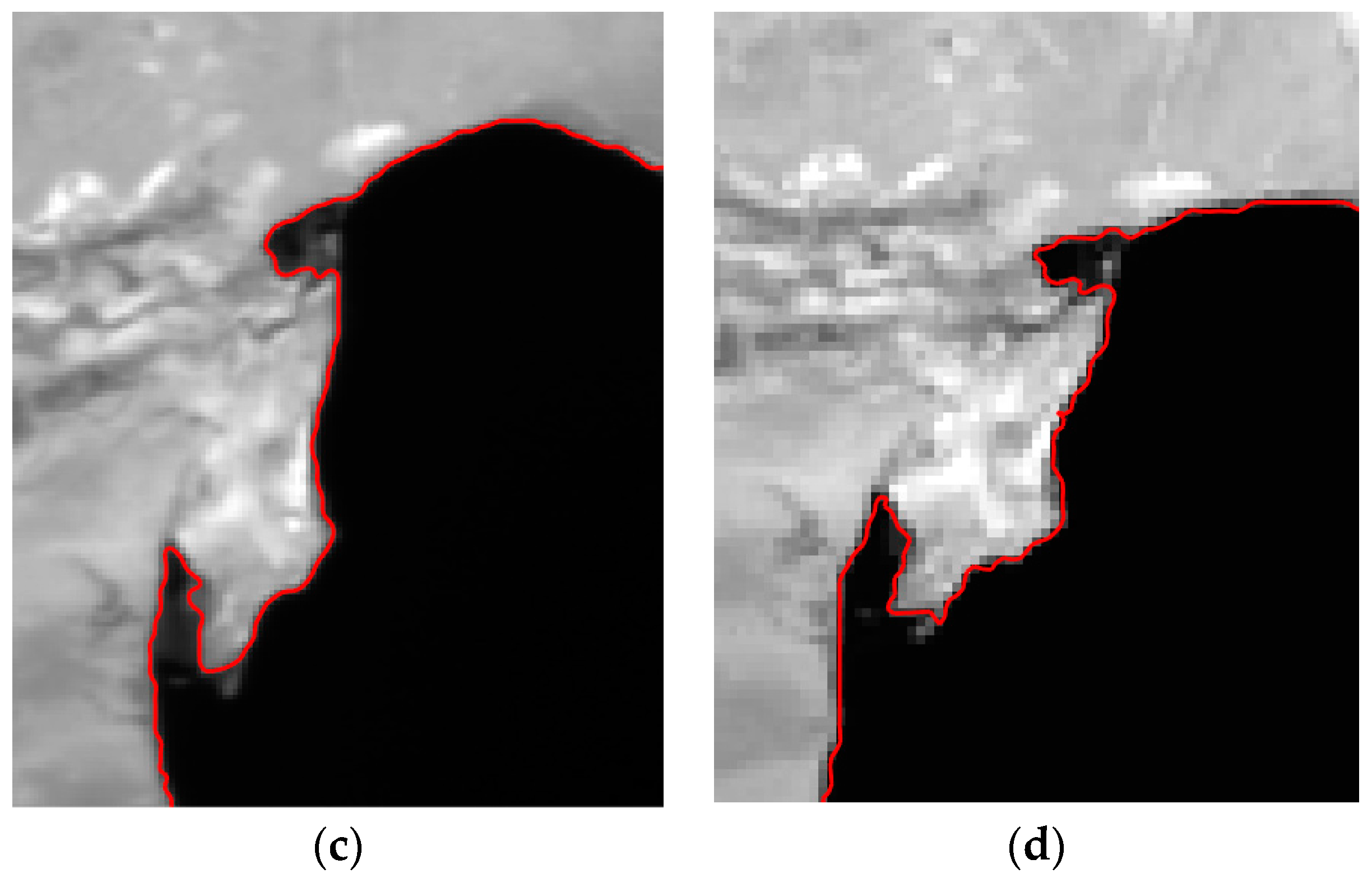
6.3.3. Effects of Spatial Resolution

To evaluate the effects of spatial resolution on the MB-Snake method, multiple images with varied spatial resolutions, including the Terra Moderate Resolution Imaging Spectroradiometer (MODIS) with the spatial resolution of 250 m and Landsat 8 operational land imager (OLI) image with the spatial resolution of 30 m, were used to compare with those of the GF-1 WFV image with the spatial resolution of 16 m. Among the extraction results of the three types of images for the same water body, GF-1 were the best with almost all of the ground object details retained, followed first by OLI, a little worse than GF-1 while still maintaining most of the object details, and then by MODIS, only salient features kept due to the poor spatial resolution. While in terms of time consumptions, GF-1 were largest, followed first by OLI and then by MODIS. The reason for this is that the external force of the MB-Snake method proposed in this paper was calculated based on the DN values of pixels, and with the improvement of the spatial resolution, the mixed pixels become fewer, and correspondingly, the values of the external forces become more appropriate, and thus the extraction results of the MB-Snake method are of higher accuracy, while the computation burden becomes heavier, and the time consumption becomes larger because of the increasing of the pixel number. The MB-Snake could theoretically be applied in images with any spatial resolution only if the water bodies are larger than one pixel. However, taking flood area determination and other specific application demands into consideration, it would be better to select satellite images with spatial resolution no lower than 30 m. The partially enlarged views of the extracted results for one of the tested images, Figure 7c, were provided in Figure 15 to prove this, with Figure 15a,c based on the image of GF-1 WFV, and Figure 15b,d based on the image of Landsat 8 OLI.

6.4. Image Demands

The MB-Snake method proposed in this paper, on the one hand, requires that there should not be heavy clouds, hazes, or noises in the satellite images as they could lead to serious confusions between the objects and their backgrounds, resulting in extraction failure, and, on the other hand, does not have high demands for the spatial resolution and band of images, and indeed it can be used in images with any spatial resolution or band only if the water bodies are large enough to be displayed in the images. However, for the same water body, the MB-Snake method has better performance and could present more boundary details on images with higher spatial resolution because there are less mixed pixels in images with higher spatial resolutions, and it would be better to select images with spatial resolution no lower than 30 m to perform water boundary extraction to meet the accuracy demands for specific applications. As for bands, it would be better to select the NIR band because it has clearer water boundaries and can ensure better extraction results when compared with other image bands.

7. Conclusions and Outlook

This paper analyzed the shortcomings of the B-Snake method, added an adaptive image preprocessing and a topology collision detection and handling mechanism, provided automatic termination criterion for the B-Snake method, and created the MB-Snake method to improve the positioning accuracy by avoiding weak boundary overflow, implement topology transformation, and perform automatic termination of contour evolution. Six types of GF-1 WFV satellite images, covering different types, sizes, complexities, and DN value contrasts, were used as experimental images. The extracted results of the MB-Snake method were compared to those of the B-Snake and OT-Snake methods to assess its feasibility and advantages. The results demonstrated that the MB-Snake method is able to efficiently prevent weak boundary overflow, detect and address topology collisions, and perform automatic termination of contour evolution, successfully meeting its design objectives and showing obvious superiority to the existing topology-flexible parametric snakes. Evaluation indexes, including correctness, completeness, and AOM, were also calculated for the B-Snake, the MB-Snake, and the OT-Snake methods to quantitatively assess and compare the performances of the MB-Snake method, and the results showed that the MB-Snake method improved the correctness, completeness, and AOM of the extracted results through the adaptive image enhancement and topology collision detection and handling schemes, reaching a conclusion that was consistent with the qualitative results. Moreover, a stability assessment was performed based on the MB-Snake method, and the results suggested that the MB-Snake method proposed in this paper is insensitive to the locations of initial contours, it is model parameter stable, and the extraction results of it will be improved with the increasing of the spatial resolution.

The MB-Snake method is good at accurately delineating the contours of given water bodies with complicated borders and multiple inner islands instead of blind water border extracting for all water bodies. This feature makes the MB-Snake method especially suitable to be applied in the determination of flood areas, providing reliable flood area decision making information support for pre-disaster risk assessment, middle-disaster rescue-plan formation, and post-disaster damage evaluation. Moreover, multiple water boundary extraction could also be achieved by cyclically calling this method many times. The MB-Snake method can also be applied in image segmentation, change detection, time-series lake or river change analysis studies, other related areas, etc. However, the MB-Snake method also has its limitations: (1) Its initial contour cannot intersect or contain the islands in the experimental images. (2) Its efficiency is not that high due to the addition of the topology detection and handling mechanism, but the time consumption for the largest of the six experimental images is about one hour, and several or tens of minutes for others (see

Table A1. Calculation efficiency of the B-Snake, the MB-Snake, and the OT-Snake methods for the six experimental images.

	Method	Efficiency(s)
Image		B-Snake	MB-Snake	OT-Snake
Figure 7a		66.1	89.4	21.2
Figure 7b		73.3	96.4	75.6
Figure 7c		2665.8	3427.8	1217.2
Figure 7d		62.8	85.7	54.6
Figure 7e		49.2	75.6	14.2
Figure 7f		1667.0	2049.8	85.7

for details), all in an acceptable level. Moreover, the efficiency can be further improved by employing computers with higher configurations or cloud computing techniques. (3) The MB-Snake was not fully automated. However, this problem can be resolved through two possible solutions: one is to automatically set the initial pixel inside the target water body via a water body judgment algorithm and meanwhile use a fixed value as radium, and the other is to acquire an initial contour automatically by a pixel clustering algorithm like seeded region growing. (4) Cloud, haze or noise removal should be firstly performed for satellite images with heavy clouds, hazes or noises. All these disadvantages will be given more attention and gradually improved in the future studies.