Change Vector Analysis to Monitor the Changes in Fuzzy Shorelines


Abstract
:
1. Introduction
2. Methodology
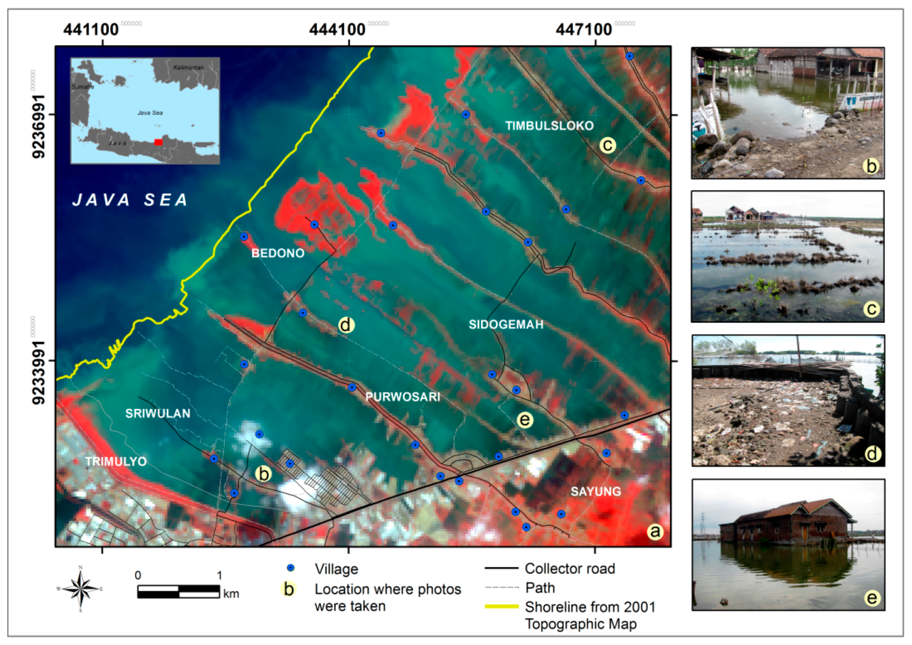
2.1. Study Area
2.2. Satellite Images, Data Pre-Processing and Reference Data Generation
2.2.1. Satellite Images and Data Pre-Processing
2.2.2. Reference Data Generation
2.3. FCM Classification
2.4. Validation
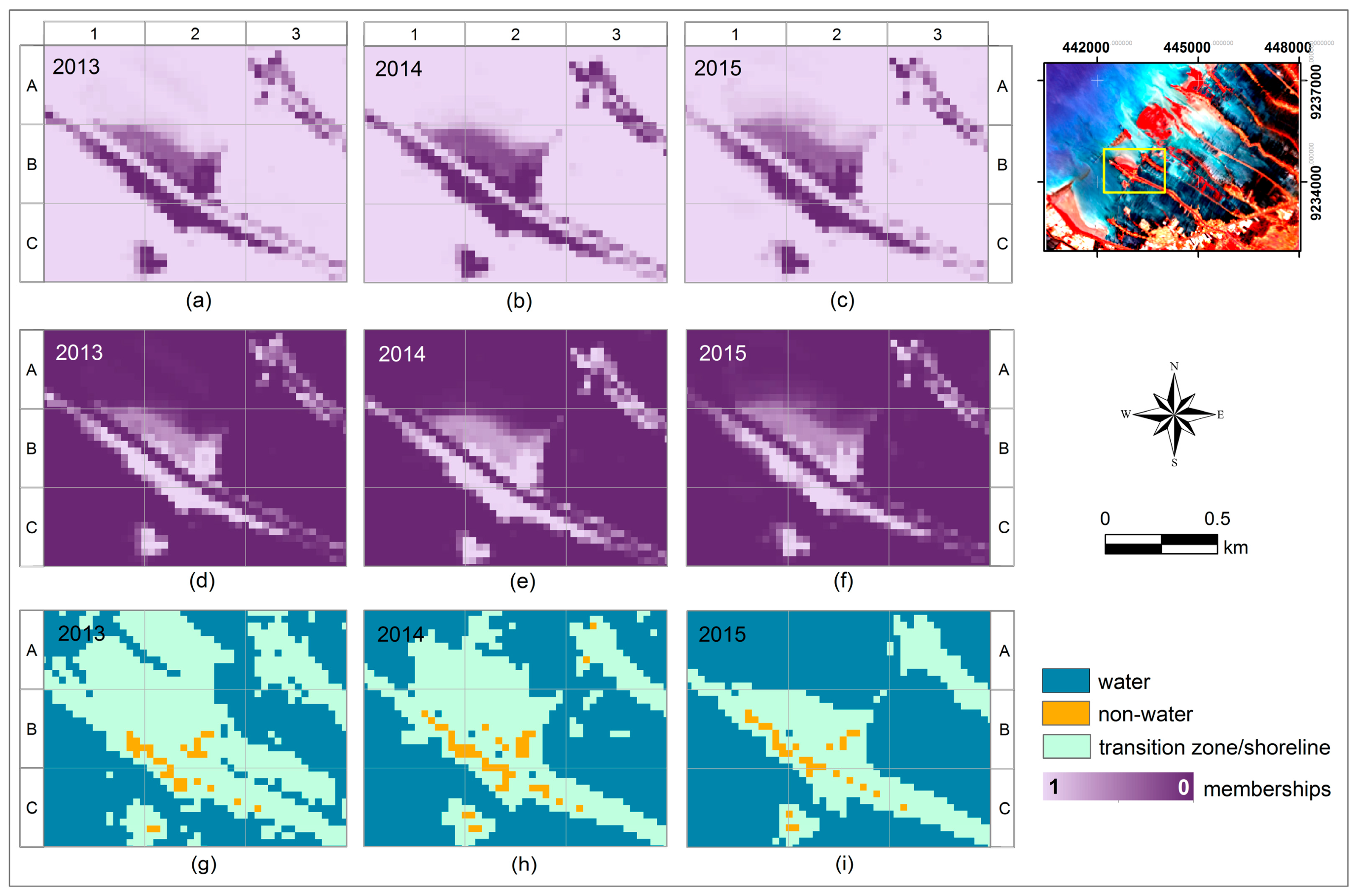
2.5. Deriving Fuzzy Shoreline
2.6. Uncertainty Estimation
2.7. Shoreline Change Detection
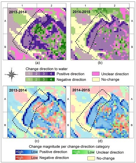
2.7.1. Change Magnitude
2.7.2. Change Direction
2.7.3. Change Uncertainty
3. Results
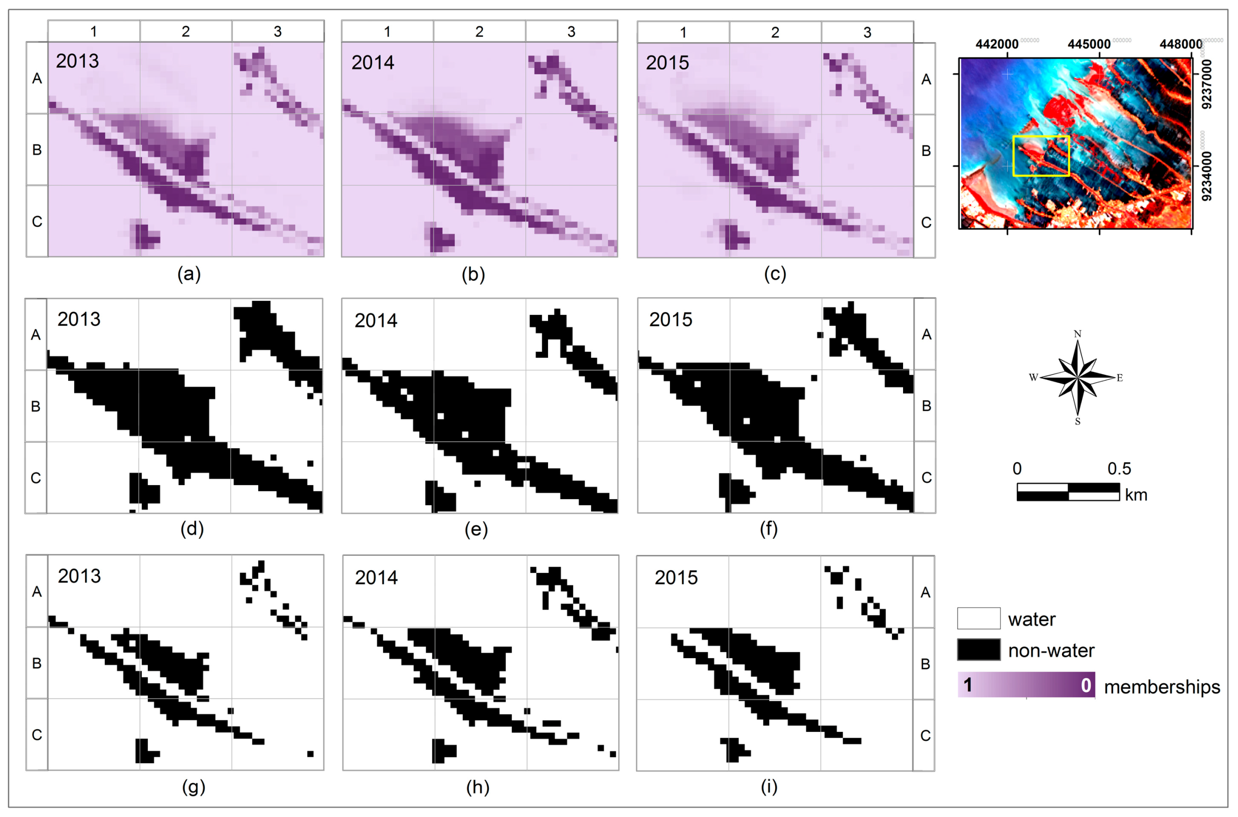
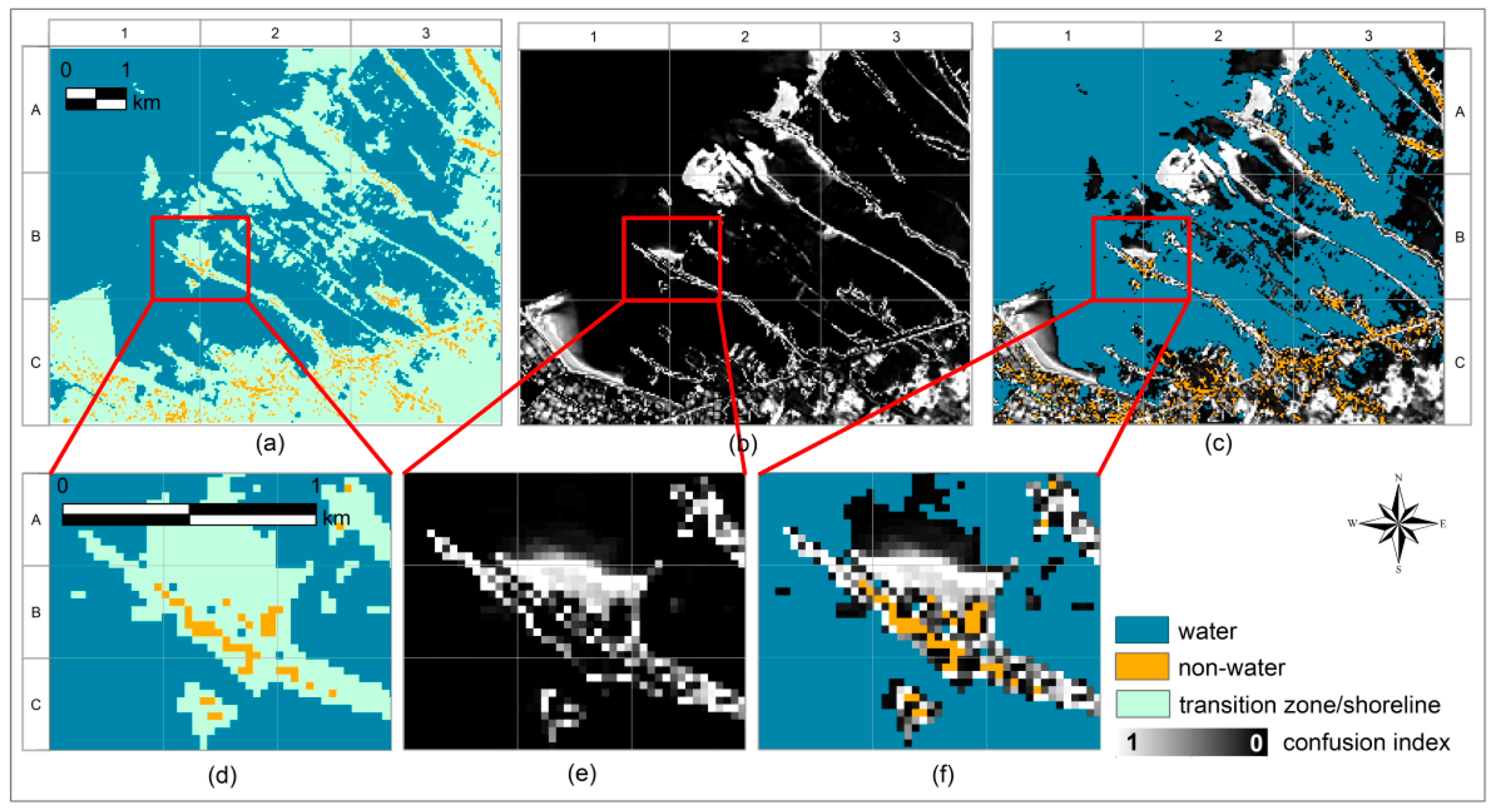
3.1. FCM Classification and Accuracy Assessment
3.2. Fuzzy Shoreline and Uncertainty Estimation
3.3. Shoreline Change Detection
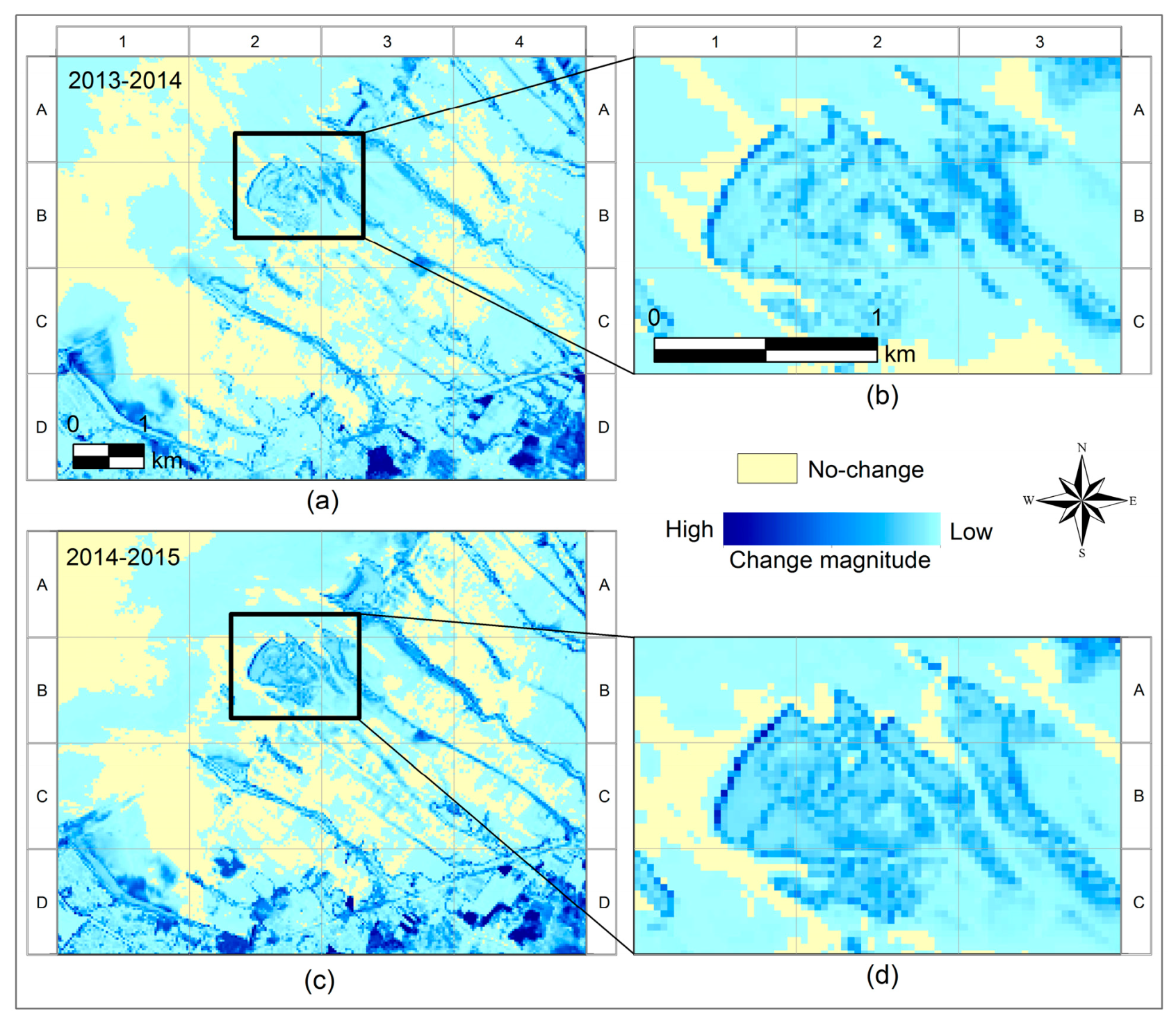
3.3.1. Change Magnitude and Change Uncertainty
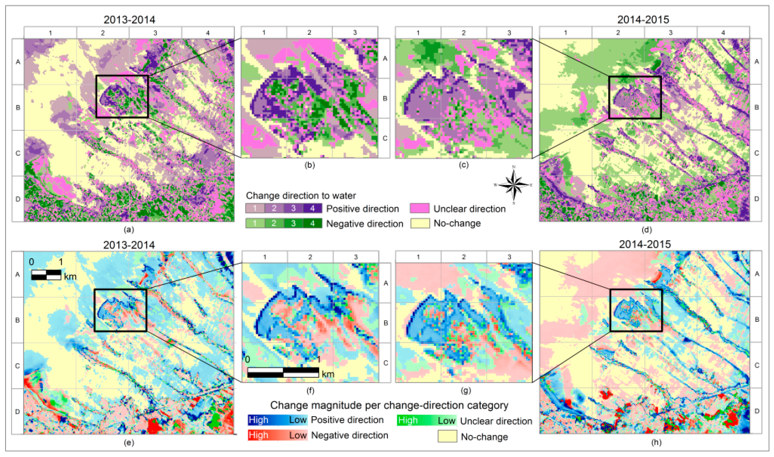
3.3.2. Change Direction
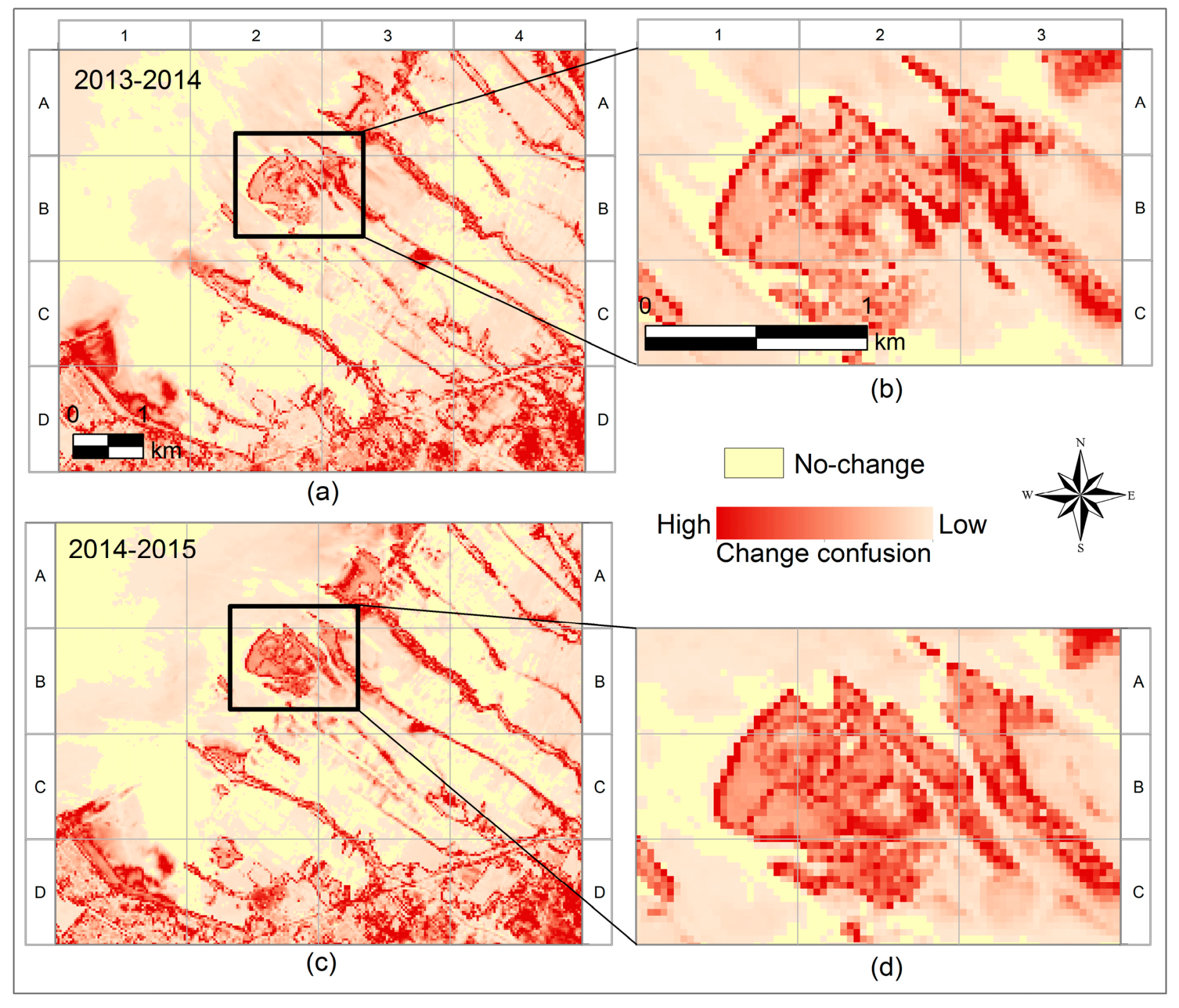
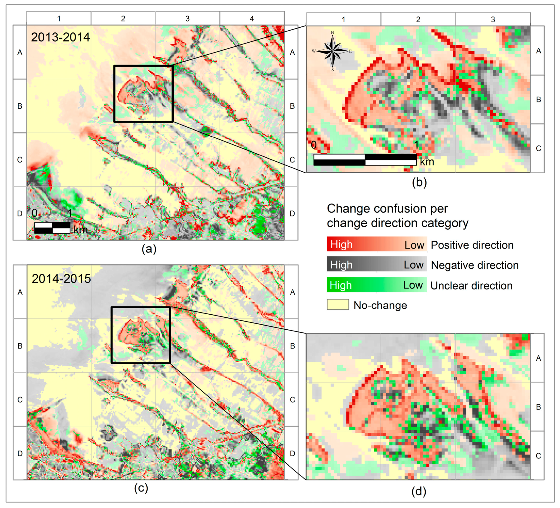
3.3.3. Change Confusion
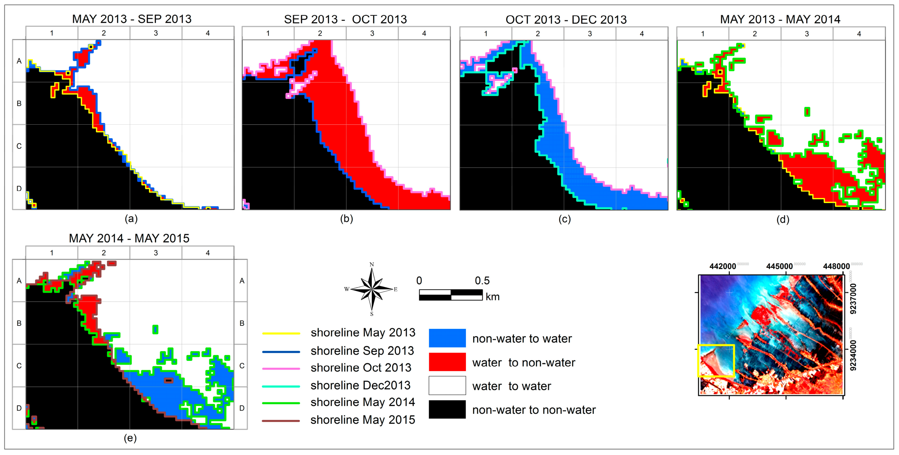
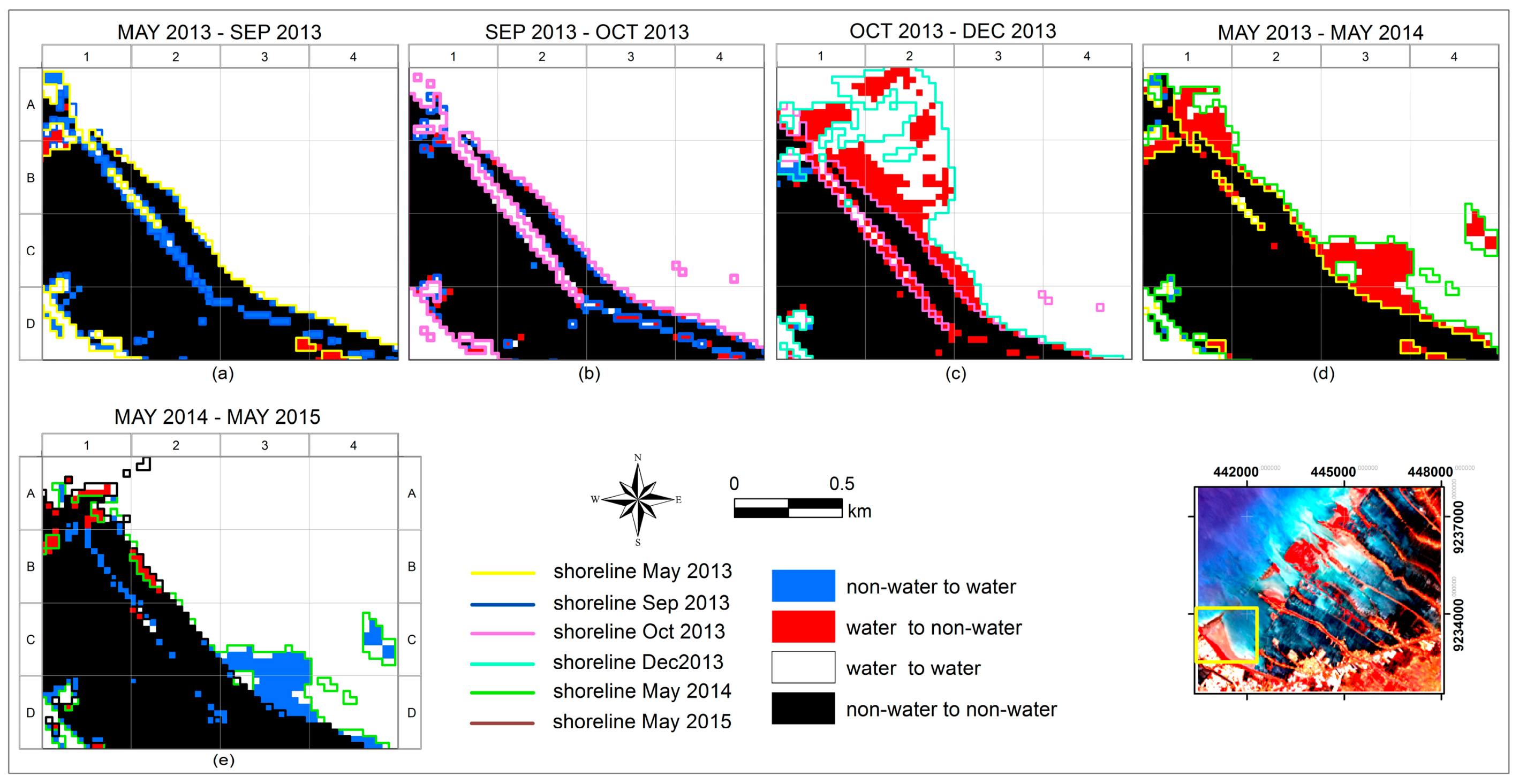
3.3.4. Comparison with Alternative Change Detection Methods
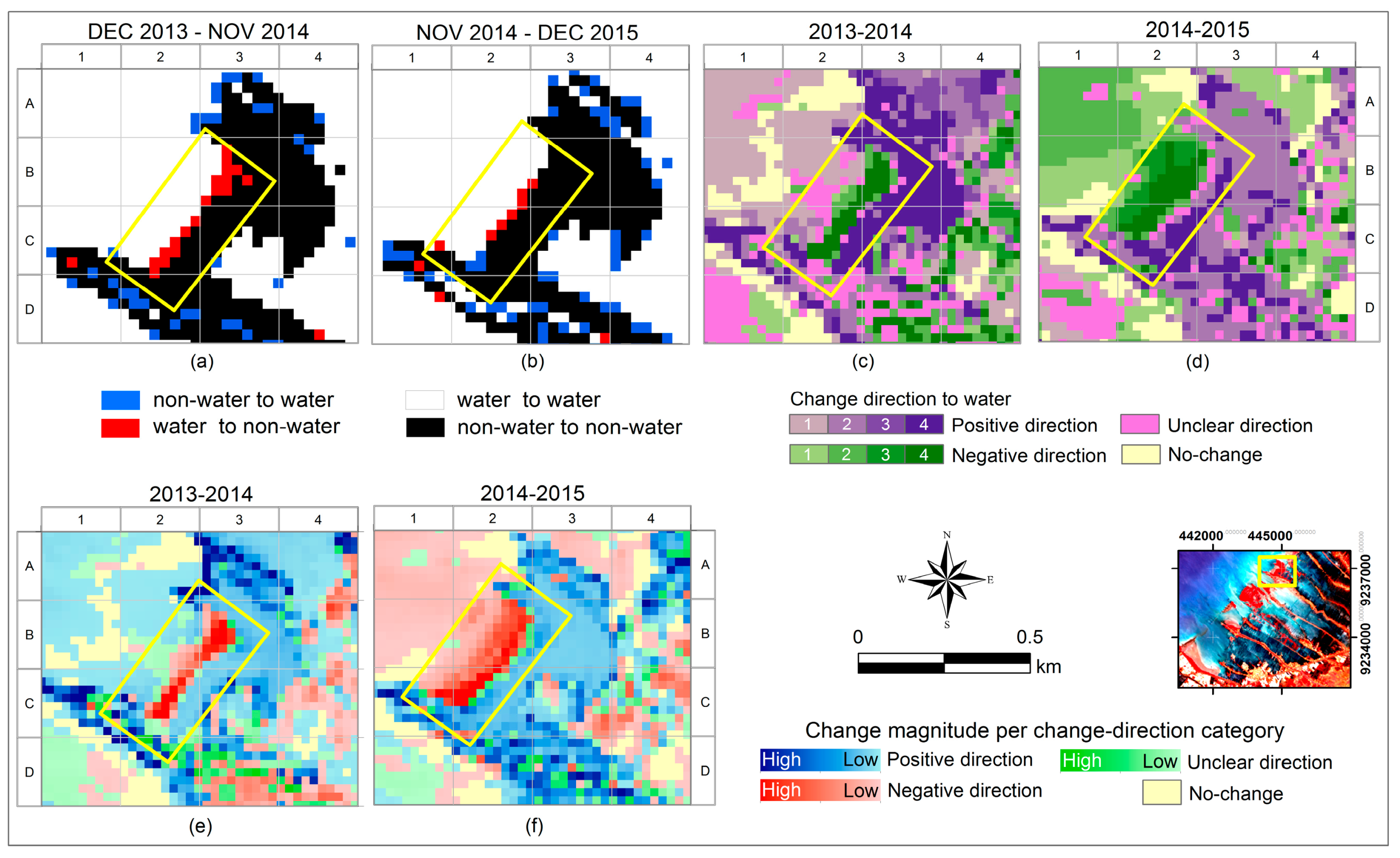
3.3.5. Multi-Year Pattern of Water Membership Changes
4. Discussion
5. Conclusions
Acknowledgments
Author Contributions
Conflicts of Interest
References
- Zanuttigh, B.; Martinelli, L.; Lamberti, A.; Moschella, P.; Hawkins, S.; Marzetti, S.; Ceccherelli, V.U. Environmental design of coastal defence in Lido di Dante, Italy. Coast. Eng. 2005, 52, 1089–1125. [Google Scholar] [CrossRef]
- Jin, D.; Hoagland, P.; Au, D.K.; Qiu, J. Shoreline change, seawalls, and coastal property values. Ocean Coast. Manag. 2015, 114, 185–193. [Google Scholar] [CrossRef]
- Baldassarre, G.D.; Schumann, G.; Bates, P.D. A technique for the calibration of hydraulic models using uncertain satellite observations of flood extent. J. Hydrol. 2009, 367, 276–282. [Google Scholar] [CrossRef]
- Kaergaard, K.; Fredsoe, J. A numerical shoreline model for shorelines with large curvature. Coast. Eng. 2013, 74, 19–32. [Google Scholar] [CrossRef]
- Snoussi, M.; Ouchani, T.; Khouakhi, A.; Niang-Diop, I. Impacts of sea-level rise on the Moroccan coastal zone: Quantifying coastal erosion and flooding in the Tangier Bay. Geomorphology 2009, 107, 32–40. [Google Scholar] [CrossRef]
- O’Connor, M.C.; Cooper, J.A.G.; McKenna, J.; Jackson, D.W.T. Shoreline management in a policy vacuum: A local authority perspective. Ocean Coast. Manag. 2010, 53, 769–778. [Google Scholar] [CrossRef]
- Tamassoki, E.; Amiri, H.; Soleymani, Z. Monitoring of shoreline changes using remote sensing (case study: Coastal city of Bandar Abbas). In 7th IGRSM International Remote Sensing & GIS Conference and Exhibition; IOP Publishing: Bristol, UK, 2014; Volume 20. [Google Scholar]
- Davidson-Arnott, R. An Introduction to Coastal Processes and Geomorphology; Cambridge University Press: Cambridge, MA, USA, 2010; p. 442. [Google Scholar]
- Bird, E.C.F. Coastline Changes: A Global Review; John Wiley & Sons: New York, NY, USA, 1985; p. 219. [Google Scholar]
- Boak, E.H.; Turner, I.L. Shoreline definition and detection: A review. J. Coast. Res. 2005, 21, 688–703. [Google Scholar] [CrossRef]
- Oertel, G.F. Coasts, coastlines, shores, and shorelines. In Encyclopedia of Coastal Science; Schwartz, M.L., Ed.; Springer: New York, NY, USA, 2005; pp. 323–327. [Google Scholar]
- Bird, E.C.F. Coastal Geomorphology: An Introduction; John Wiley & Sons: Chicester, UK, 2000. [Google Scholar]
- Liu, X.; Xia, J.C.; Blenkinsopp, C.; Arnold, L.; Wright, G. High Water Mark Determination Based on the Principle of Spatial Continuity of the Swash Probability. J. Coast. Res. 2014, 30, 487–499. [Google Scholar] [CrossRef]
- Moore, L.J.; Ruggiero, P.; List, J.H. Comparing Mean High Water and High Water Line Shorelines: Should Proxy-Datum Offsets be Incorporated into Shoreline Change Analysis? J. Coast. Res. 2006, 22, 894–905. [Google Scholar] [CrossRef]
- Ghosh, M.K.; Kumar, L.; Roy, C. Monitoring the coastline change of Hatiya Island in Bangladesh using remote sensing techniques. ISPRS J. Photogramm. 2015, 101, 137–144. [Google Scholar] [CrossRef]
- Dewi, R.S.; Bijker, W.; Stein, A.; Marfai, M.A. Fuzzy Classification for Shoreline Change Monitoring in a Part of the Northern Coastal Area of Java, Indonesia. Remote Sens. 2016, 8, 1–25. [Google Scholar] [CrossRef]
- Fisher, P.F. Models of uncertainty in spatial data. Geogr. Inf. Syst. 1999, 1, 191–205. [Google Scholar]
- Li, R.; Ma, R.; Di, K. Digital tide-coordinated shoreline. Mar. Geod. 2002, 25, 27–36. [Google Scholar] [CrossRef]
- Senthilnatha, J.; H, V.S.; Omkar, S.N.; Mani, V. Spectral-spatial MODIS image analysis using swarm intelligence algorithms and region based segmentation for flood assessment. In Proceedings of the Seventh International Conference on Bio-Inspired Computing: Theories and Applications; Bansal, J.C., Singh, P.K., Deep, K., Pant, M., Nagar, A.K., Eds.; Springer: New Delhi, India, 2012. [Google Scholar]
- Marfai, M.A.; Almohammad, H.; Dey, S.; Susanto, B.; King, L. Coastal dynamic and shoreline mapping: Multi-sources spatial data analysis in Semarang Indonesia. Environ. Monit. Assess. 2008, 142, 297–308. [Google Scholar] [CrossRef] [PubMed]
- Shenbagaraj, N.; Mani, N.D.; Muthukumar, M. Isodata classification technique to assess the shoreline changes of Kolachel to Kayalpattanam coast. Int. J. Eng. Res. Technol. 2014, 3. [Google Scholar]
- Muslim, A.M.; Foody, G.M.; Atkinson, P.M. Localized soft classification for super-resolution mapping of the shoreline. Int. J. Remote Sens. 2006, 27, 2271–2285. [Google Scholar] [CrossRef]
- Taha, L.G. E.-d.; Elbeih, S.F. Investigation of fusion of SAR and Landsat data for shoreline super resolution mapping: The Northeastern Mediterranean sea coast in Egypt. Appl. Geomat. 2010, 2, 177–186. [Google Scholar] [CrossRef]
- Jianya, G.; Haigang, S.; Guorui, M.; Qiming, Z. A Review of Multi-Temporal Remote Sensing Data Change Detection Algorithms. Int. Arch. Photogramm., Remote Sens. Spat. Inf. Sci. 2008, 37, 757–762. [Google Scholar]
- Lambin, E.F.; Strahler, A.H. Change-Vector Analysis in Multitemporal Space: A Tool to Detect and Categorize Land-Cover Change Processes Using High Temporal-Resolution Satellite Data. Remote Sens. Environ. 1994, 48, 231–244. [Google Scholar] [CrossRef]
- Singh, A. Digital Change Detection Techniques using Remotely-Sensed Data. Int. J. Remote Sens. 1989, 10, 989–1003. [Google Scholar] [CrossRef]
- Lu, D.; Li, G.; Moran, E. Current situation and needs of change detection techniques. Int. J. Image Data Fusion 2014, 5, 13–38. [Google Scholar] [CrossRef]
- Kauth, R.J.; Thomas, G.S. The Tasselled Cap—A Graphic Description of the Spectral-Temporal Development of Agricultural Crops as Seen by Landsat; LARS Symposia; Purdue University: Lafayette, IN, USA, 1976; pp. 41–51. [Google Scholar]
- Malila, W.A. Change Vector Analysis: An Approach for Detecting Forest Changes with Landsat; LARS Symposia; Purdue University: Lafayette, IN, USA, 1980. [Google Scholar]
- Lambin, E.F.; Ehrlich, D. Land-cover Changes in Sub-Saharan Africa (1982–1991): Application of a Change Index Based on Remotely Sensed Surface Temperature and Vegetation Indices at a Continental Scale. Remote Sens. Environ. 1997, 64, 181–200. [Google Scholar] [CrossRef]
- Landmann, T.; Schramm, M.; Huettich, C.; Dech, S. MODIS-based change vector analysis for assessing wetland dynamics in Southern Africa. Remote Sens. Lett. 2013, 42, 104–113. [Google Scholar] [CrossRef]
- Vorovencii, I. A change vector analysis technique for monitoring land cover changes in Copsa Mica, Romania, in the period 1985–2011. Environ. Monit. Assess. 2014, 186, 5951–5968. [Google Scholar] [CrossRef] [PubMed]
- He, C.; Wei, A.; Shi, P.; Zhang, Q.; Zhao, Y. Detecting land-use/land-cover change in rural–urban fringe areas using extended change-vector analysis. Int. J Appl. Earth Obs. Geoinf. 2011, 13, 572–585. [Google Scholar] [CrossRef]
- Singh, S.; Talwar, R. Performance Analysis of Different Threshold Determination Techniques for Change Vector Analysis. J. Geol. Soc. India 2015, 86, 52–58. [Google Scholar] [CrossRef]
- Özyavuz, M.; Satir, O.; Bilgili, B.C. A Change Vector Analysis Technique to Monitor Land-Use/Land-Cover in the Yildiz Mountains, Turkey. Fresenius Environ. Bull. 2011, 20, 1190–1199. [Google Scholar]
- Hartini, S. Flood Risk Modelling on Agricultural Area in the North Coastal Area of Central Java. Ph.D. Thesis, Gadjah Mada University, Yogyakarta, Indonesia, 2015. [Google Scholar]
- Marfai, M.A. Preliminary assessment of coastal erosion and local community adaptation in Sayung coastal area, Central Java–Indonesia. Quaest. Geogr. 2012, 31, 47–55. [Google Scholar]
- Harwitasari, D.; van Ast, J.A. Climate change adaptation in practice: People’s responses to tidal flooding in Semarang, Indonesia. J. Flood Risk Manag. 2011, 4, 216–233. [Google Scholar] [CrossRef]
- Marfai, M.A.; King, L.; Sartohadi, J.; Sudrajat, S.; Budiani, S.R.; Yulianto, F. The impact of tidal flooding on a coastal community in Semarang, Indonesia. Environmentalist 2008, 28, 237–248. [Google Scholar] [CrossRef]
- Sarbidi. Rob influence on Coastal Settlements (Case Study: Semarang City). In Losses in Buildings and Areas Due Sea-level Rise on Coastal Cities in Indonesia, Bandung, 19–20 March 2001; Research Center for Settlements, Ministry of Public Works: Bandung, Indonesia, 2001. [Google Scholar]
- Kurniawan, L. Tidal flood assessment in Semarang (case: Dadapsari). Alami 2003, 8, 54–59. [Google Scholar]
- Marfai, M.A.; King, L. Tidal inundation mapping under enhanced land subsidence in Semarang, Central Java Indonesia. Nat. Hazards 2007, 44, 93–109. [Google Scholar] [CrossRef]
- USGS United States Geological Survey. Available online: https://earthexplorer.usgs.gov/ (accessed on 22 November 2015).
- Hadjimitsis, D.G.; Papadavid, G.; Agapiou, A.; Themistocleous, K.; Hadjimitsis, M.G.; Retalis, A.; Michaelides, S.; Chrysoulakis, N.; Toulios, L.; Clayton, C.R.I. Atmospheric correction for satellite remotely sensed data intended for agricultural applications: Impact on vegetation indices. Nat. Hazards Earth. Syst. Sci. 2010, 10, 89–95. [Google Scholar] [CrossRef]
- Mather, P.M. Computer Processing of Remotely-Sensed Images: An Introduction, 3rd ed.; John Wiley & Sons: Chicester, UK, 2004; p. 352. [Google Scholar]
- Lu, D.; Weng, Q. A survey of image classification methods and techniques for improving classification performance. Int. J. Remote Sens. 2007, 28, 823–870. [Google Scholar] [CrossRef]
- Congalton, R.G.; Green, K. Assessing the Accuracy of Remotely Sensed Data : Principles and Practices, 2nd ed.; CRC Press: Boca Raton, FL, USA, 2009. [Google Scholar]
- Pontius, R.G.; Cheuk, M.L. A generalized cross-tabulation matrix to compare soft-classified maps at multiple resolutions. Int. J. Geogr. Inf. Sci. 2006, 20, 1–30. [Google Scholar] [CrossRef]
- Harikumar, A.; Kumar, A.; Stein, A.; Raju, P.L.N.; Murthy, Y.V.N.K. An effective hybrid approach to remote-sensing image classification. Int. J. Remote Sens. 2015, 36, 2767–2785. [Google Scholar] [CrossRef]
- Bezdek, J.C.; Ehrlich, R.; Full, W. FCM: The fuzzy c-means clustering algorithm. Comput. Geosci. 1984, 10, 191–203. [Google Scholar] [CrossRef]
- Burrough, P.A. Fuzzy mathematical methods for soil survey and land evaluation. J. Soil Sci. 1989, 40, 477–492. [Google Scholar] [CrossRef]
- Cheng, T. Fuzzy Objects: Their Changes and Uncertainties. Photogramm. Eng. Remote Sens. 2002, 68, 41–49. [Google Scholar]
- Zhu, A.-X.; Yang, L.; Li, B.; Qin, C.; Pei, T.; Liu, B. Construction of membership functions for predictive soil mapping under fuzzy logic. Geoderma 2010, 155, 164–174. [Google Scholar] [CrossRef]
- Chuang, K.-S.; Tzeng, H.-L.; Chen, S.; Wu, J.; Chen, T.-J. Fuzzy c-means clustering with spatial information for image segmentation. Comput. Med. Image Graph. 2006, 30, 9–15. [Google Scholar] [CrossRef] [PubMed]
- Medasani, S.; Kim, J.; Krishnapuram, R. An overview of membership function generation techniques for pattern recognition. Int. J. Approx. Reason. 1998, 19, 391–417. [Google Scholar] [CrossRef]
- Silván-Cárdenas, J.L.; Wang, L. Sub-pixel confusion–uncertainty matrix for assessing soft classifications. Remote Sens. Environ. 2008, 112, 1081–1095. [Google Scholar] [CrossRef]
- Binaghi, E.; Brivio, P.A.; Ghezzi, P.; Rampini, A. A fuzzy set-based accuracy assessment of soft classification. Pattern Recognit. Lett. 1999, 20, 935–948. [Google Scholar] [CrossRef]
- Richards, J.A. Remote Sensing Digital Image Analysis, 5th ed.; Springer: New York, NY, USA, 2013. [Google Scholar]
- Wang, F. Fuzzy Supervised Classification of Remote Sensing Images. IEEE Trans. Geosci. Remote Sens. 1990, 28, 194–201. [Google Scholar] [CrossRef]
- Dutta, A. Fuzzy c-Means Classification of Multispectral Data Incorporating Spatial Contextual Information by Using Markov Random Field; ITC: Enschede, The Netherlands, 2009. [Google Scholar]
- Zhang, J.; Foody, G.M. A fuzzy classification of sub-urban land cover from remotely sensed imagery. Int. J. Remote Sens. 1998, 19, 2721–2738. [Google Scholar] [CrossRef]
- Tso, B.; Mather, P. Classification Methods for Remotely Sensed Data; CRC Press: Boca Raton, FL, USA, 2009; p. 347. [Google Scholar]
- Burrough, P.A.; van Gaans, P.F.M.; Hootsmans, R. Continuous classification in soil survey: Spatial correlation, confusion and boundaries. Geoderma 1997, 77, 115–135. [Google Scholar] [CrossRef]
- Cheng, T.; Molenaar, M.; Lin, H. Formalizing fuzzy objects from uncertain classification results. Int. J. Geogr. Inf. Sci. 2001, 15, 27–42. [Google Scholar] [CrossRef]
- Zhang, J.; Kirby, R.P. Alternative Criteria for Defining Fuzzy Boundaries Based on Fuzzy Classification of Aerial Photographs and Satellite Images. Photogramm. Eng. Remote Sens. 1999, 65, 1379–1387. [Google Scholar]
- Lunetta, R.S.; Elvidge, C.D. Remote Sensing Change Detection: Environmental Monitoring Methods and Applications; Taylor & Francis: London, UK, 1999. [Google Scholar]
- Zhang, J.; Foody, G.M. Fully-fuzzy Supervised Classification of sub-urban Land Cover from Remotely Sensed Imagery: Statistical and Artificial Neural Network Approaches. Int. J. Remote Sens. 2001, 22, 615–628. [Google Scholar] [CrossRef]
- Bijker, W.; Hamm, N.A.; Ijumulana, J.; Wole, M.K. Monitoring a fuzzy object: The case of Lake Naivasha. In Proceedings of the 6th International Workshop on the Analysis of Multi-Temporal Remote Sensing Images (Multi-Temp), Trento, Italy, 12–14 July 2011.
- Wang, Q.; Shi, W. Unsupervised classification based on fuzzy c-means with uncertainty analysis. Remote Sens. Lett. 2013, 4. [Google Scholar] [CrossRef]
- Fisher, P.F.; Pathirana, S. The evaluation of fuzzy membership of land cover classes in the suburban zone. Remote Sens. Environ. 1990, 34, 121–132. [Google Scholar] [CrossRef]
- Zarandi, M.H.F.; Faraji, M.R.; Karbasian, M. An exponential cluster validity index for fuzzy clustering with crisp and fuzzy data. Trans. E Ind. Eng. 2010, 17, 95–110. [Google Scholar]
- Delinom, R.M.; Assegaf, A.; Abidin, H.Z.; Taniguchi, M.; Suherman, D.; Lubis, R.F.; Yulianto, E. The contribution of human activities to subsurface environment degradation in Greater Jakarta Area, Indonesia. Sci. Total Environ. 2008, 407, 3129–3141. [Google Scholar] [CrossRef] [PubMed]
- Molenaar, M.; Cheng, T. Fuzzy spatial objects and their dynamics. ISPRS J. Photogramm. 2000, 55, 164–175. [Google Scholar] [CrossRef]
- Pugh, D.T. Tides, Surges and Mean Sea-Level; John Wiley & Sons: London, UK, 1987. [Google Scholar]
- Chawla, S. Possibilistic C-Means—Spatial Contextual Information Based Sub-Pixel Classification Approach for Multi-Spectral Data. Master’s Thesis, University of Twente, Enschede, The Netherlands, 2010. [Google Scholar]
- Foody, G.M. Status of land cover classification accuracy assessment. Remote Sens. Environ. 2002, 80, 185–201. [Google Scholar] [CrossRef]
- Dean, R.G.; Dalrymple, R.A. Coastal Processes: With Engineering Applications; Cambridge University Press: Cambridge, MA, USA, 2002; p. 473. [Google Scholar]
- Netherlands-Water-Partnership, Indonesia—The Netherlands integrated approach of future water challenges. In Water for Food and Ecosystems: Using the Power of Nature; Braak, B.T. (Ed.) Netherlands Water Partnership (NWP): Den Haag, The Netherlands, 2016; pp. 26–30.
- Winterwerp, H.; van Wesenbeeck, B.; van Dalfsen, J.; Tonneijck, F.; Astra, A.; Verschure, S.; van Eijk, P. A Sustainable Solution for Massive Coastal Erosion in Central Java; Discussion Paper; Deltares: Delft, The Netherlands, 2014; pp. 1–45. [Google Scholar]


| Acquisition Date | Astronomical Tide Level (m) | Reference Data | Acquisition Date | Astronomical Tide Level (m) | Reference Data |
|---|---|---|---|---|---|
| 23 May 2013 | −0.1 | Pleiades (27 February 2013) | 29 May 2015 | +0.04 | Sentinel 2 (26 December 2015) |
| 12 September 2013 | −0.1 | 18 September 2015 | −0.1 | ||
| 14 October 2013 | −0.3 | 20 October 2015 | −0.3 | ||
| 1 December 2013 | −0.3 | 21 November 2015 | −0.3 | ||
| 10 May 2014 | −0.01 | Spot 6 (5 October 2014) | |||
| 15 September 2014 | −0.2 | ||||
| 1 October 2014 | −0.2 | ||||
| 18 November 2014 | −0.3 |
| Satellite | Bands | Wavelength (μm) | Satellite | Bands | Wavelength (μm) |
|---|---|---|---|---|---|
| Landsat 8 OLI/TIRS | Coastal and Aerosol | 0.43–0.45 | SPOT 6 | Blue | 0.45–0.52 |
| Blue | 0.45–0.51 | Green | 0.53–0.59 | ||
| Green | 0.53–0.59 | Red | 0.625–0.695 | ||
| Red | 0.64–0.67 | NIR | 0.76–0.89 | ||
| NIR | 0.85–0.88 | ||||
| SWIR 1 | 1.57–1.65 | ||||
| SWIR 2 | 2.11–2.29 | ||||
| Pleiades | Blue | 0.43–0.55 | Sentinel 2 | Blue | 0.49 |
| Green | 0.50–0.62 | Green | 0.56 | ||
| Red | 0.59–0.71 | Red | 0.665 | ||
| NIR | 0.74–0.94 | SWIR | 0.842 |
| CC | CV | TCV | Chg.Dir | CC | CV | TCV | Chg.Dir | ||||||
|---|---|---|---|---|---|---|---|---|---|---|---|---|---|
| CV1 | CV2 | CV3 | CV4 | CV1 | CV2 | CV3 | CV4 | ||||||
| 1 | 0 | 0 | 0 | 0 | 0 | No-change | 41 | 0 | +1 | 0 | −1 | 0 | Unclear direction |
| 2 | +1 | +1 | +1 | +1 | +4 | Positive direction | 42 | +1 | 0 | 0 | −1 | 0 | Unclear direction |
| 3 | +1 | 0 | +1 | +1 | +3 | Positive direction | 43 | 0 | 0 | −1 | +1 | 0 | Unclear direction |
| 4 | 0 | +1 | +1 | +1 | +3 | Positive direction | 44 | 0 | −1 | 0 | +1 | 0 | Unclear direction |
| 5 | +1 | +1 | 0 | +1 | +3 | Positive direction | 45 | −1 | +1 | +1 | −1 | 0 | Unclear direction |
| 6 | +1 | +1 | +1 | 0 | +3 | Positive direction | 46 | +1 | −1 | +1 | −1 | 0 | Unclear direction |
| 7 | +1 | −1 | +1 | +1 | +2 | Positive direction | 47 | +1 | −1 | −1 | +1 | 0 | Unclear direction |
| 8 | −1 | +1 | +1 | +1 | +2 | Positive direction | 48 | −1 | +1 | −1 | +1 | 0 | Unclear direction |
| 9 | +1 | +1 | −1 | +1 | +2 | Positive direction | 49 | +1 | +1 | −1 | −1 | 0 | Unclear direction |
| 10 | +1 | +1 | +1 | −1 | +2 | Positive direction | 50 | −1 | −1 | +1 | +1 | 0 | Unclear direction |
| 11 | 0 | +1 | +1 | 0 | +2 | Positive direction | 51 | 0 | −1 | 0 | 0 | −1 | Negative direction |
| 12 | +1 | 0 | +1 | 0 | +2 | Positive direction | 52 | −1 | 0 | 0 | 0 | −1 | Negative direction |
| 13 | +1 | 0 | 0 | +1 | +2 | Positive direction | 53 | 0 | 0 | −1 | 0 | −1 | Negative direction |
| 14 | 0 | +1 | 0 | +1 | +2 | Positive direction | 54 | 0 | 0 | 0 | −1 | −1 | Negative direction |
| 15 | +1 | +1 | 0 | 0 | +2 | Positive direction | 55 | 0 | +1 | −1 | −1 | −1 | Negative direction |
| 16 | 0 | 0 | +1 | +1 | +2 | Positive direction | 56 | 0 | −1 | +1 | −1 | −1 | Negative direction |
| 17 | +1 | 0 | 0 | 0 | +1 | Positive direction | 57 | −1 | +1 | 0 | −1 | −1 | Negative direction |
| 18 | 0 | +1 | 0 | 0 | +1 | Positive direction | 58 | −1 | 0 | +1 | −1 | −1 | Negative direction |
| 19 | 0 | 0 | 0 | +1 | +1 | Positive direction | 59 | +1 | 0 | −1 | −1 | −1 | Negative direction |
| 20 | 0 | 0 | +1 | 0 | +1 | Positive direction | 60 | +1 | −1 | 0 | −1 | −1 | Negative direction |
| 21 | 0 | +1 | −1 | +1 | +1 | Positive direction | 61 | 0 | −1 | −1 | +1 | −1 | Negative direction |
| 22 | 0 | −1 | +1 | +1 | +1 | Positive direction | 62 | −1 | −1 | +1 | 0 | −1 | Negative direction |
| 23 | −1 | +1 | 0 | +1 | +1 | Positive direction | 63 | +1 | −1 | −1 | 0 | −1 | Negative direction |
| 24 | −1 | 0 | +1 | +1 | +1 | Positive direction | 64 | −1 | +1 | −1 | 0 | −1 | Negative direction |
| 25 | +1 | 0 | −1 | +1 | +1 | Positive direction | 65 | −1 | −1 | 0 | +1 | −1 | Negative direction |
| 26 | +1 | −1 | 0 | +1 | +1 | Positive direction | 66 | −1 | 0 | −1 | +1 | −1 | Negative direction |
| 27 | +1 | 0 | +1 | −1 | +1 | Positive direction | 67 | 0 | 0 | −1 | −1 | −2 | Negative direction |
| 28 | +1 | −1 | +1 | 0 | +1 | Positive direction | 68 | −1 | 0 | −1 | 0 | −2 | Negative direction |
| 29 | +1 | +1 | 0 | −1 | +1 | Positive direction | 69 | 0 | −1 | −1 | 0 | −2 | Negative direction |
| 30 | +1 | +1 | −1 | 0 | +1 | Positive direction | 70 | −1 | −1 | 0 | 0 | −2 | Negative direction |
| 31 | 0 | +1 | +1 | −1 | +1 | Positive direction | 71 | 0 | −1 | 0 | −1 | −2 | Negative direction |
| 32 | −1 | +1 | +1 | 0 | +1 | Positive direction | 72 | −1 | 0 | 0 | −1 | −2 | Negative direction |
| 33 | 0 | +1 | −1 | 0 | 0 | Unclear direction | 73 | +1 | −1 | −1 | −1 | −2 | Negative direction |
| 34 | 0 | −1 | +1 | 0 | 0 | Unclear direction | 74 | −1 | +1 | −1 | −1 | −2 | Negative direction |
| 35 | −1 | +1 | 0 | 0 | 0 | Unclear direction | 75 | −1 | −1 | −1 | +1 | −2 | Negative direction |
| 36 | −1 | 0 | +1 | 0 | 0 | Unclear direction | 76 | −1 | −1 | +1 | −1 | −2 | Negative direction |
| 37 | +1 | 0 | −1 | 0 | 0 | Unclear direction | 77 | 0 | −1 | −1 | −1 | −3 | Negative direction |
| 38 | +1 | −1 | 0 | 0 | 0 | Unclear direction | 78 | −1 | 0 | −1 | −1 | −3 | Negative direction |
| 39 | 0 | 0 | +1 | −1 | 0 | Unclear direction | 79 | −1 | −1 | −1 | 0 | −3 | Negative direction |
| 40 | −1 | 0 | 0 | +1 | 0 | Unclear direction | 80 | −1 | −1 | 0 | −1 | −3 | Negative direction |
| 81 | −1 | −1 | −1 | −1 | −4 | Negative direction | |||||||
| Classified Images | Overall Accuracy | ||
|---|---|---|---|
| FCM | MLC | Hardened Classification | |
| 23 May 2013 | 0.87 | 0.72 | 0.86 |
| 12 September 2013 | 0.85 | 0.76 | 0.85 |
| 14 October 2013 | 0.86 | 0.73 | 0.86 |
| 1 December 2013 | 0.86 | 0.73 | 0.84 |
| 10 May 2014 | 0.89 | 0.78 | 0.87 |
| 15 September 2014 | 0.90 | 0.76 | 0.88 |
| 1 October 2014 | 0.90 | 0.78 | 0.88 |
| 18 November 2014 | 0.91 | 0.79 | 0.90 |
| 29 May 2015 | 0.84 | 0.75 | 0.84 |
| 18 September 2015 | 0.88 | 0.79 | 0.87 |
| 20 October 2015 | 0.89 | 0.79 | 0.86 |
| 21 November 2015 | 0.89 | 0.80 | 0.88 |
| Change Category | 2013–2014 | 2014–2015 |
|---|---|---|
| Positive direction | 1828 | 1120 |
| Negative direction | 920 | 1635 |
| Unclear direction | 616 | 528 |
| No-change | 1319 | 1403 |
© 2017 by the authors. Licensee MDPI, Basel, Switzerland. This article is an open access article distributed under the terms and conditions of the Creative Commons Attribution (CC BY) license ( http://creativecommons.org/licenses/by/4.0/).
Share and Cite
Dewi, R.S.; Bijker, W.; Stein, A. Change Vector Analysis to Monitor the Changes in Fuzzy Shorelines. Remote Sens. 2017, 9, 147. https://doi.org/10.3390/rs9020147
Dewi RS, Bijker W, Stein A. Change Vector Analysis to Monitor the Changes in Fuzzy Shorelines. Remote Sensing. 2017; 9(2):147. https://doi.org/10.3390/rs9020147
Chicago/Turabian StyleDewi, Ratna Sari, Wietske Bijker, and Alfred Stein. 2017. "Change Vector Analysis to Monitor the Changes in Fuzzy Shorelines" Remote Sensing 9, no. 2: 147. https://doi.org/10.3390/rs9020147
APA StyleDewi, R. S., Bijker, W., & Stein, A. (2017). Change Vector Analysis to Monitor the Changes in Fuzzy Shorelines. Remote Sensing, 9(2), 147. https://doi.org/10.3390/rs9020147