Article

Using UAS Hyperspatial RGB Imagery for Identifying Beach Zones along the South Texas Coast

Texas A&M University-Corpus Christi, Corpus Christi, TX 78412, USA
*
Author to whom correspondence should be addressed.
Remote Sens. 2017, 9(2), 159; https://doi.org/10.3390/rs9020159
Submission received: 18 November 2016 / Revised: 25 January 2017 / Accepted: 10 February 2017 / Published: 15 February 2017
(This article belongs to the Special Issue Recent Trends in UAV Remote Sensing)

Abstract

:
Shoreline information is fundamental for understanding coastal dynamics and for implementing environmental policy. The analysis of shoreline variability usually uses a group of shoreline indicators visibly discernible in coastal imagery, such as the seaward vegetation line, wet beach/dry beach line, and instantaneous water line. These indicators partition a beach into four zones: vegetated land, dry sand or debris, wet sand, and water. Unmanned aircraft system (UAS) remote sensing that can acquire imagery with sub-decimeter pixel size provides opportunities to map these four beach zones. This paper attempts to delineate four beach zones based on UAS hyperspatial RGB (Red, Green, and Blue) imagery, namely imagery of sub-decimeter pixel size, and feature textures. Besides the RGB images, this paper also uses USGS (the United States Geological Survey) Munsell HSV (Hue, Saturation, and Value) and CIELUV (the CIE 1976 (L*, u*, v*) color space) images transformed from an RGB image. The four beach zones are identified based on the Gray Level Co-Occurrence Matrix (GLCM) and Local Binary Pattern (LBP) textures. Experiments were conducted with South Padre Island photos acquired by a Nikon D80 camera mounted on the US-16 UAS during March 2014. The results show that USGS Munsell hue can separate land and water reliably. GLCM and LBP textures can slightly improve classification accuracies by both unsupervised and supervised classification techniques. The experiments also indicate that we could reach acceptable results on different photos while using training data from another photo for site-specific UAS remote sensing. The findings imply that parallel processing of classification is feasible.

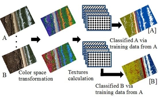
Graphical Abstract

1. Introduction

The coast comprises the interface between land and sea, and the shoreline is represented by the margin between the two [1]. At any given time, an instantaneous shoreline position is influenced by the short-term effect of the tide and a wide variety of long term effects such as relative sea-level rise and along shore littoral sediment movement [2,3]. Due to the dynamic nature of the shoreline coast, investigators often use shoreline indicators to represent the true shoreline position [4]. The three widely used indicators include seaward dune vegetation line, wet/dry line, and instantaneous water line. These indicators partition a beach into four zones from fore dune to sea, including vegetated land, dry sand or debris, wet sand, and water. The four beach zones have different spectral and geometric properties so that they are visibly discernible on coastal imagery. The vegetation line is the extreme seaward boundary of natural vegetation that spreads continuously inland and is typically used to determine the landward extent of the public beach [5]. The wet/dry line can be interpreted on both color and grey scale aerial photographs [2,6,7]. The wet/dry line represents the landward extent of the most recent high tide and is characterized by a change in sand color due to repeated, periodic inundation by high tides [4]. The instantaneous water line is naturally defined as the water position on imagery at imaging time.
The hyperspatial UAS (Unmanned Aircraft System) imagery, namely imagery of sub-decimeter pixel size, has been used for coastal surveying [8]. For example, coastal topography and change were examined with the structure from motion approach [9,10,11,12]. The beach composition (sand, rubble, and rocks) and sub-surface classes (seagrass, sand, algae, and rocks) were identified by using the digital surface models and ortho-photos derived from the UAS data [13]. Although the hyperspatial UAS imagery has been used for coastal studies in recent years, there has been little examination of this data source for beach zones and shoreline studies. This paper explores a novel method to delineate four beach zones based on UAS hyperspatial RGB (Red, Green, and Blue) imagery and textures. On the one hand, the RGB true-color imagery has been used for mapping aquatic vegetation with the object-based image analysis [14] and adaptive cosine estimator and spectral angle mapper algorithm [15]. The RGB wide band images acquired by typical off-the-shelf cameras, such as those found in small UAS remote sensing units, limits the use of conventional remote sensing spectral indexes, however, the UAS hyperspatial imagery allows geometric properties such as textures to be used with classification algorithms. This paper investigates different color space transformations from the UAS RGB imagery on beach zone classification.
On the other hand, the gray level co-occurrence matrices (GLCM) textures [16], the most used texture for remote sensing classification [17,18], have been extensively used [18,19]. This paper evaluates GLCM textures and the local binary pattern (LBP) to identify the four beach zones. The LBP [20] has already obtained great success in computer vision and pattern recognition in recent years [21]. In this paper, the four beach zones along the south Texas Gulf coast were identified through GLCM and LBP texture features using four widely used classification techniques, including the iterative self-organizing data analysis technique (ISODATA), maximum likelihood classification (MLC), the random forests (RF), and support vector machine (SVM). All of the photos for the analysis were obtained during a short period to ensure the atmospheric conditions were the same for each photo. This paper investigates the feasibility of using the training data from one photo for classification on other photos without radiation calibration or brightness balance among the photos.

2. Background

2.1. Experiment Site

The experiment area is the beach of South Padre Island, a barrier island along the Texas Gulf Coast (Figure 1). South Padre Island experiences a humid subtropical climate with the average annual high of 27.2 °C and the average low of 19.1 °C. The average annual precipitation is 73.7 cm, and the rainfall tends to be the highest during the summer and autumn months. At the Padre Island, wind-driven tides are much more important than astronomical tides [22]. Wind stress coupled with changes in barometric pressure often raises or lowers water levels on Gulf of Mexico beaches as much as 1 m [23]. Astronomical tides average about 40 cm [24] and range from 45 cm to 60 cm [25]. Sediments deposited high on the Gulf beach are dried and transported landward by persistent onshore winds. This migrating sand is trapped along the back edge of the beach by salt-tolerant grasses and flowering plants. The vegetation stabilizes the sand with roots and spreading vines, forming a relatively continuous dune ridge. However, the vegetation on dunes can be easily damaged by human activities.

2.2. Color Features

Color is perceived by humans as a combination of primary colors, R (red), G (green) and B (blue). From RGB representation, we can derive other kinds of color representations (spaces) by using either linear or nonlinear transformations. Several color spaces, such as RGB, HSV (Hue, Saturation, and Value), and CIELUV (the CIE 1976 (L*, u*, v*) color space), are widely utilized in color image segmentation. The HSV (Hue-Saturation-Value) color space can be illustrated as a conical object in the three-dimensional form. Hue is represented by the circular part of the cone. Saturation is calculated using the radius of the cone,and Value is the height of the cone. CIELUV, which is an abbreviation of the CIE 1976 (L*, u*, v*) color space, was developed by the International Commission on Illumination (CIE) in 1976 to represent perceptual uniformity. CIELUV meets the psychophysical need for a human observer. For an application, selecting the best color space is still one of the difficulties in color image segmentation [26,27]. Standard RGB (sRGB) is a standard RGB color space created for use on the Internet, computers, and printers. Digital cameras usually use sRGB as the default working color space. While RGB is suitable for color display, it is not good for color scene segmentation and analysis due to the high correlation among the R, G, and B components [26,27].
The Munsell color system created by Albert H. Munsell was modified by the U. S. Geological Survey (USGS) to describe color in digital images [28]. The modified Munsell color system is called USGS Munsell HSV color space. Here, RGB coordinates also are transformed into the color coordinates Hue, Saturation, and Value (HSV). Hue is expressed as the angle around the central vertical axis from 0 to 360 degrees, where 0 and 360 = blue, 120 = green, and 240 = red. Saturation is the amount of gray (0% to 100%) in the color; 0 means that the color is gray; and 100% means that the color is a primary color. Value is the brightness of the color and varies with color saturation. It also ranges from 0% to 100%. When Value is 0, the color space will be totally black. With the increase in the value, the color space brightness up and shows various colors. Neutral grays lie along the vertical axis between black and white. This paper uses all of these color spaces including RGB, CIELUV, and USGS Munsell HSV color spaces.

2.3. Texture Features

The similar land objects may have similar geometric patterns as manifested by grey-level variation in an image, which is referred to as texture. Among numerous texture measures, the gray level co-occurrence matrices (GLCM) [16] is the most used texture for remote sensing classification [17,18]. Local binary pattern (LBP) is a new rotation invariant texture analysis method which is theoretically simple but very powerful [21].
Let g ( ρ 1 , ρ 2 , h , θ ) be the relative occurrence of pixels with grey levels ρ 1 and ρ 2 spaced h pixels apart in direction θ. Relative occurrence is the total number of times each grey level pair is counted, divided by the total possible number of grey level pairs. The GLCM for a region, defined by a user-specified window, is the matrix of those measurements over all grey level pairs [29]. Generally, the bigger the window size, the coarser the information that can be provided by texture features. If there are L grey-level values possible, then the GLCM will be an L × L matrix. Given that L can be quite large, the brightness value can be binned. The displacement (h) commonly uses one pixel due to the highly correlated spatial relationship between one pixel and its neighbor. The GLCM computed for various values of θ are kept separate to see whether the texture is orientation dependent. The common directions are horizontal, vertical, and diagonal. The commonly used eightGLCM parameters include mean, variance, contrast, homogeneity, dissimilarity, entropy, angular second moment (energy), and correlation. GLCM variance is a measure of the dispersion of the values around the GLCM mean. The range of homogeneity is [0, 1]. If the image has little variation, then homogeneity is high, and if there is no variation, then homogeneity is equal to 1. If the neighboring pixels are very similar in their grey level values, then the contrast in the image is very low. High contrast values are expected for heavy textures and low values for smooth textures.
LBP operator is defined in a circle local neighborhood. With grey-level of the center pixel as the threshold, the circular neighbors at a certain radius R are labeled as 1 if the neighbor has greater grey-level than the center or 0. Then, the binary values are multiplied by the corresponding weights according to their positions. The LBP code of the center pixel is the sum of the weighted binary values. For a circularly symmetric neighbor set defined by LBP, where R = 1, and P = 8, g0, g2, g4, and g6 are neighbor pixels at left, upper, right, and lower, respectively. While g1, g3, g5, g7 are interpolated on the four diagonal directions. The uniformity measure U is defined in Equation (1).
U ( L B P P , R ) = i = 1 P | s ( g i g c ) s ( g i 1 g c ) |
where g P = g 0 . g c and g i denote the grey level of the center pixel and the neighbor pixel, respectively. s(x) is the sign function. P is the number of pixels around the center pixel and R represents the radius of the circular neighborhood. Patterns with a U value of less than or equal to two are designated as “uniform”. Further, a rotation invariant uniform LBP is defined as:
L B P P , R r i u 2 = { i = 1 P s ( g i g c )   i f   U 2 P + 1   o t h e r w i s e
Any uniform pattern is calculated by counting ones in the binary number, while all the non-uniform patterns are labeled as P + 1. Multi-scale LBP can be calculated by various P and R. Common combinations of P and R are: P = 8, R = 1; P = 16, R = 2; and P = 24, R = 3.

2.4. Classification Techniques

The following four classification techniques, iterative self-organizing data analysis Technique (ISODATA), maximum likelihood classification (MLC), support vector machine (SVM), and random forest (RF), are widely used by the remote sensing community.
ISODATA is an unsupervised classification that merges clusters if their separation distance in multispectral feature space is less than a user-specified value and includes the rules for splitting a single cluster into two clusters. This method makes a large number of passes through the dataset until specified results are obtained [30,31].
MLC is the most commonly supervised classification method used with remote sensing image data. The MLC algorithm is based on the Bayes’ theorem of decision making and assumes that the points of each class sample follow normal distribution. With this assumption, a class response pattern can be characterized by the mean vector and the covariance matrix. The statistical probability of a given pixel is computed for each class to determine the membership of the pixel to the class. When the default equal option for a priori probability weighting is specified, a pixel is assigned to the class to which it has the highest probability of being a member.
SVM, an advanced supervised classification, generates a separating hyperplane by only those pixels in its vicinity optimal for the available training data. For linearly non-separable data, a transformation of the pixel vector x to a higher order feature space can be applied that renders the data linearly separable. The radial basis function (RBF) kernel exp ( γ x i x j 2 ) is commonly used for transformation in remote sensing data. For classification tasks, SVM C-classification with the RBF kernel is suitable due to its good general performance and the few number of parameters (only two: C and γ ) [32,33,34]. The C parameter controls the tradeoff between achieving a low training error and achieving a low testing error which is the ability to generalize the classifier to unseen data. The γ parameter defines how far the influence of a single training example reaches, with low values meaning ‘far’ and high values meaning ‘close’. The best combination of C and γ is often selected by a grid search of C and γ [35]. Typically, the parameters with best cross-validation accuracy are selected.
RF, also called random decision forests [36], is an ensemble learning method for supervised classification. Random forests construct a multitude of decision trees at training time and outputs the class that is the mode of the classes of the individual trees. Random forests use out-of-bag (OOB) error as an estimation of the generalization error [37,38]. The number of trees is a free parameter. An optimal number of trees can be found by observing the out-of-bag error. The OOB error is convergent when the number of trees is bigger than a certain threshold [34]. Another free parameter is the number of randomly selected predictor variables, which typically is the square root of the number of input variables for classification [39].

3. Materials and Methods

3.1. UAS Data

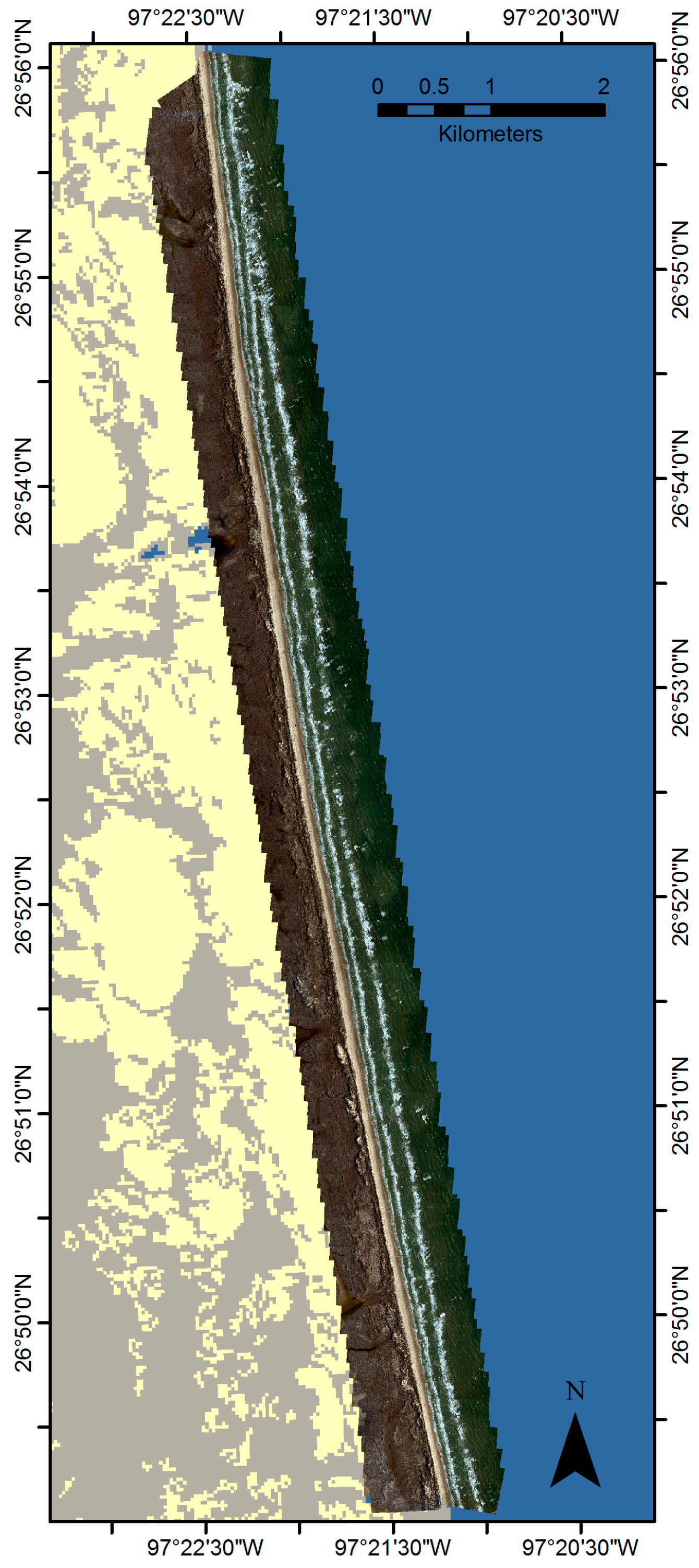
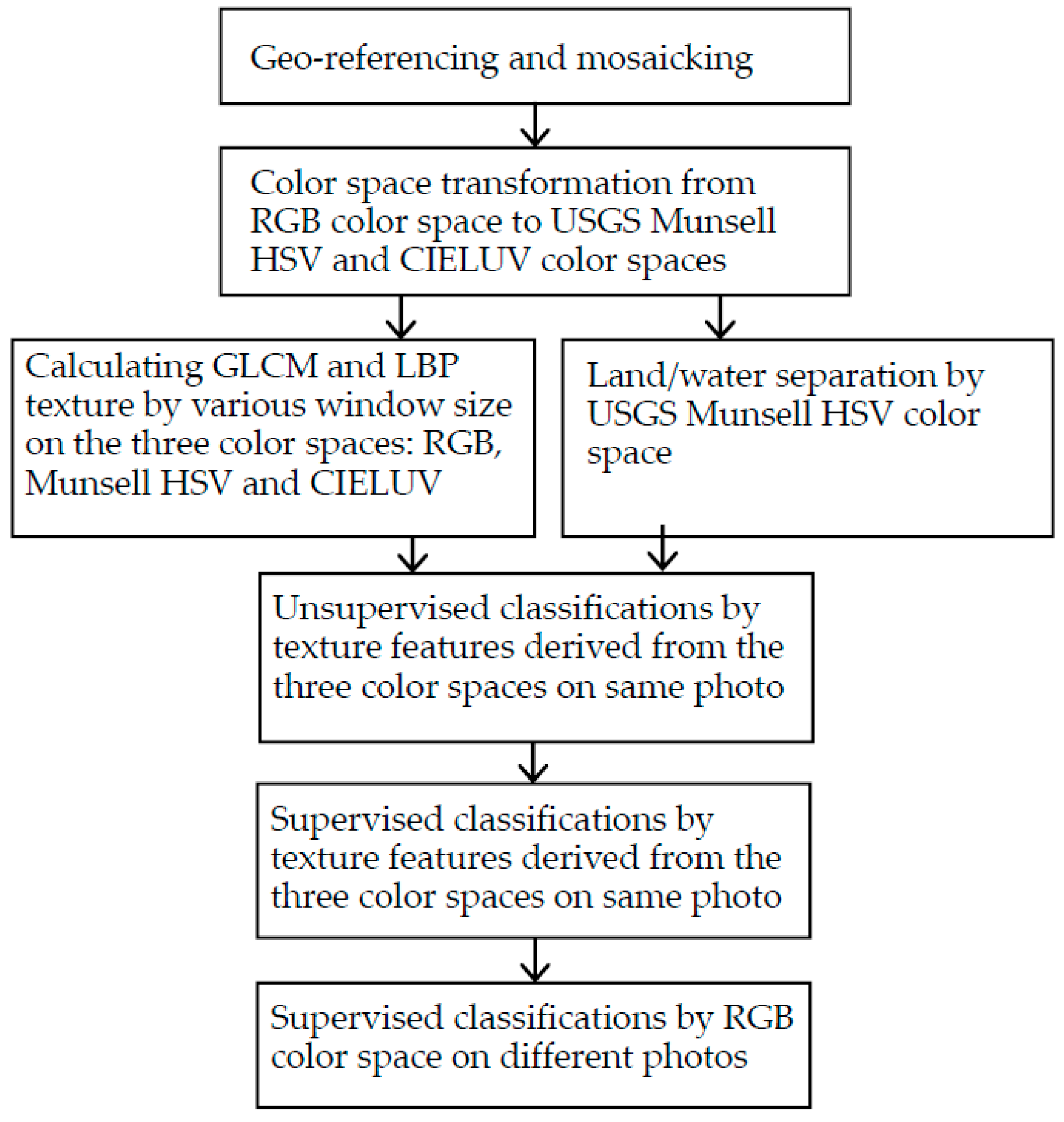
The UAS images were acquired along 12.9 km of shoreline on 4 March 2014 using an American Aerospace RS-16 owned by the Texas A&M University-Corpus Christi (TAMU-CC) Unmanned Aircraft Systems Program, and with the support of the TAMU-CC Lone Star UAS Center of Excellence and Innovation. The March exercise used a Nikon D800 camera with a 50 mm focal length and 0.0049 mm charge-coupled device (CCD) pixel size. The flight height was 870 m above the ground. In total, there are 402 overlapping photos with 10 cm ground pixels; the photos were acquired during 30 min with three flight paths. To rapidly process hundreds of UAS photos, a two-stage approach was developed. First, we produced ortho-images of 1-m pixel size with raw exterior orientation data and conducted co-registration with translation to produce a 1-m resolution mosaic image. Second, using the 1-m mosaic as a spatial constraint, we refined co-registration by adjusting the exterior orientation parameters. The final mosaic image consists of the ortho-images of 10 cm pixel size (Figure 2). The workflow of the beach zone classification is displayed in Figure 3.

3.2. Sea and Land Separation by USGS Munsell Color System

3.2.1. Interaction of Light and Water and USGS Munsell Color Characteristics

As sunlight penetrates a water body, energy at the red band is absorbed more than energy at the blue band. As a result, water pixels are predominantly blue and green so that water pixels have hues less than 150 in USGS Munsell HSV color space. Land pixels have 180 to 300 hue due to bare soil and plant litter being largely yellow and brown. Therefore, water pixels have lower hue than land pixels in the USGS Munsell color space. The shadows on land generated by terrain and the ones on the sea created by waves are dark. The white foam is white. Both the shadows and the white foam have very low hue values in the USGS Munsell color space. The USGS Munsell Value is low for shadows and high for sand beach. As a result, five classes were identified using the USGS Munsell color space, and they are vegetated land, sea, shadows, white foam, and sand beach. Their characteristics are summarized in Table 1. This paper uses MATLAB to implement CIELUV color space transformation and ENVI to conduct USGS Munsell HSV color space transformation.

3.2.2. Separation of Water and Land

Initially, the extraction of water was performed by labeling all pixels with Munsell hue that are higher than a defined threshold to the class of water. The distribution of the Munsell hue of water and no-water typically is a bi-modal mixture distribution. We used the Gaussian mixture model (GMM), a suitable model to separate two classes [40], to separate water and land. The GMM is a probabilistic model that assumes all the data points are generated from a mixture of a finite number of Gaussian distributions with unknown parameters. For example, for the one-dimensional data, the parameters to be found are a mean and variance for each component. Based on the previous section, we set 60 and 200 as the initial means for water and land. For that purpose, we used the GMM algorithm to perform the thresholding that is set by a hue with 1.0 probability for land and 0 probability for water.
The morphology Open operation with an adequate window such as a 31 × 31 pixel window (approximate 3 m × 3 m) was used to eliminate mislabeled water pixels. This size is empirical. It is worthy to note that very shallow waters on the swash zone are commonly labeled as land because the bottom sediment is clear on the UAS photos. Therefore, a sufficient large buffer was generated for the water pixels. A distance of 80 meters (approximate 800 pixels) is adopted to split the image pixels into two categories; namely, sea or land. This cut distance was obtained from our knowledge of the south Texas shorelines. This separation of land and sea is robust because it is based on the difference of light interactions with land and water. No manual editing was needed in this classification, though a little tuning was done. Due to limited space, a full description on the fuzzy-set based classification is not presented here, but it is available upon request.

3.3. ISODATA Identification of Beach Zones with Texture Features on the Same Photo

Co-relationship between the commonly used GLCM parameters were investigated in order to find independent parameters. The experiments show that there are three distinguished groups: variance, contrast, and a group including all others, namely homogeneity, dissimilarity, entropy, and energy. The GLCM mean is independent to the three groups. GLCM correlation cannot contribute to the classification. The experiments with horizontal, vertical, and diagonal orientation showed that orientation dependence of the textures is weak. Therefore, only diagonal dependence of the texture is used in the experiments.
The highest classification accuracy can be achieved by the inclusion of the optimal scale of textures where ground objects represent the highest between-class variation and the lowest within-class variation [18]. To analyze how the accuracy changes with texture window size, we tested five different sizes: 3 × 3, 7 × 7, 15 × 15, 31 × 31, and 63 × 63. The four GLCM parameters, namely mean, variance, contrast, and homogeneity, were derived at all the five window sizes on five bands, namely RGB bands, L of CIELUV and Value of USGS Munsell HSV. Then, they were added separately as additional ancillary bands to the five band images for the unsupervised classification experiments.
Similarly, the LBP and variance at different resolutions were derived on the five bands, and added separately as additional ancillary bands for classification experiments. LBP and variance were calculated by three resolutions, samples = 8 or 16, and radius = 1, 3, 5. In total, LBP and variance were computed at five scales as follows: P = 8, R = 1 (scale 1), P = 8, R = 2 (scale 2), P = 8, R = 3 (scale 3a), P = 16, R = 3 (scale 3b), and P = 8, R = 5 (scale 5).
The unsupervised ISODATA classification algorithm was used to partition an image, consisting of a color band and additional texture features, into clusters. With the aid of the sea and land image produced by Munsell color space, each cluster was assigned to one of the four beach zones according to the labeling rules: vegetated land, dry sand, wet sand, and water. One hundred fourteen points on the beach images were randomly selected and were visual interpreted as ground reference. The confusion matrix was calculated for each classification experiment.

3.4. Supervised Classification for Beach Zones with Texture Features on the Same Photo

The three supervised classification methods, MLC, SVM, and RF, were used to classify beach zones with texture features on the same photo. The texture features used by the supervised classifications are the same as the ones used in the previous section. In summary, both the GLCM parameters at the five window sizes and the LBP parameters at the five scales were derived on the five bands, and then added independently as additional ancillary bands to the five band images for the classifications. The test dataset in the previous section was used to calculate the confusion matrix and total accuracy. The training set was generated by drawing areas of interest on a photo for each of four classes, and then randomly selecting approximately 1000 pixels from the areas for each class.
The SVM C-classification with the RBF kernel was conducted under the R statistical computing environment with package e1071. The RF classification was conducted under the R statistical computing environment with package randomForest.

3.5. Beach Zone Classification in Different Photos Using a Training Set from Another Photo

In general, remote sensing classification training data are from the same image. If one wants to use training data for an extended area, good radiation calibration or brightness balance is necessary for all images in the extended area. This is because satellite images are usually acquired under different atmospheric conditions. However, for a site-specific UAS observation, for example, 10 km range, all photos can be acquired within a short period. Thus, we can assume that the atmospheric conditions remain the same. Our results showed the training data from one photo for another photo classification is feasible. Three photos were used here. One (DSC_7559) is from the middle of the flight; the other two photos (DSC_7479 and DSC_7611) are from the beginning and end of the flight, respectively. The training data was from photo DSC7559 and the classification was conducted on DSC7479 and DSC7611. To evaluate the accuracy, three classification methods, MLC, SVM, and RF, were performed. One hundred seven points on DSC-7611 and 116 points on DSC_7479 were randomly chosen and visually interpreted as the ground reference. The confusion matrix was calculated for each classification experiment. The distance between training data and target photos are approximately 6km. The distance between the two target photos is approximately 12 km.

4. Results and Discussions

4.1. Accuracies of Unsupervised Classification

To evaluate the accuracy improvement by the texture features, classifications of the original five color space bands, namely red, green, blue, L of CIELUV and Value of USGS Munsell HSV, were first conducted. The classification results (Table 2) are considered as a baseline for the further texture classifications. Table 3 and Table 4 show the accuracy of the three GLCM textures on RGB bands and on the Value of the USGS Munsell HSV and the L of the CIELUV. Table 5 shows the accuracy of the LBP of the five scales by the five color space bands. Here, the labeling rules for contrast and homogeneity on the five bands are the same for all the five window sizes. The GLCM variance for the 3 × 3 and 7 × 7 windows also use the same labeling rules for contrast and homogeneity. The LBP texture uses the same rules for each scale.
As shown in Table 2, the red band has the best performance among the five color space bands for the beach zone identification. As shown in Table 3, except the window of 63 × 63 pixels, the results by homogeneity and contrast are affected slightly by the window size, while the variance performance decreases when window size increases for all three bands. The homogeneity performance is the best among the three texture factors, and the contrast is better than the variance. The red contrast on the 15 × 15 window size has the best results.
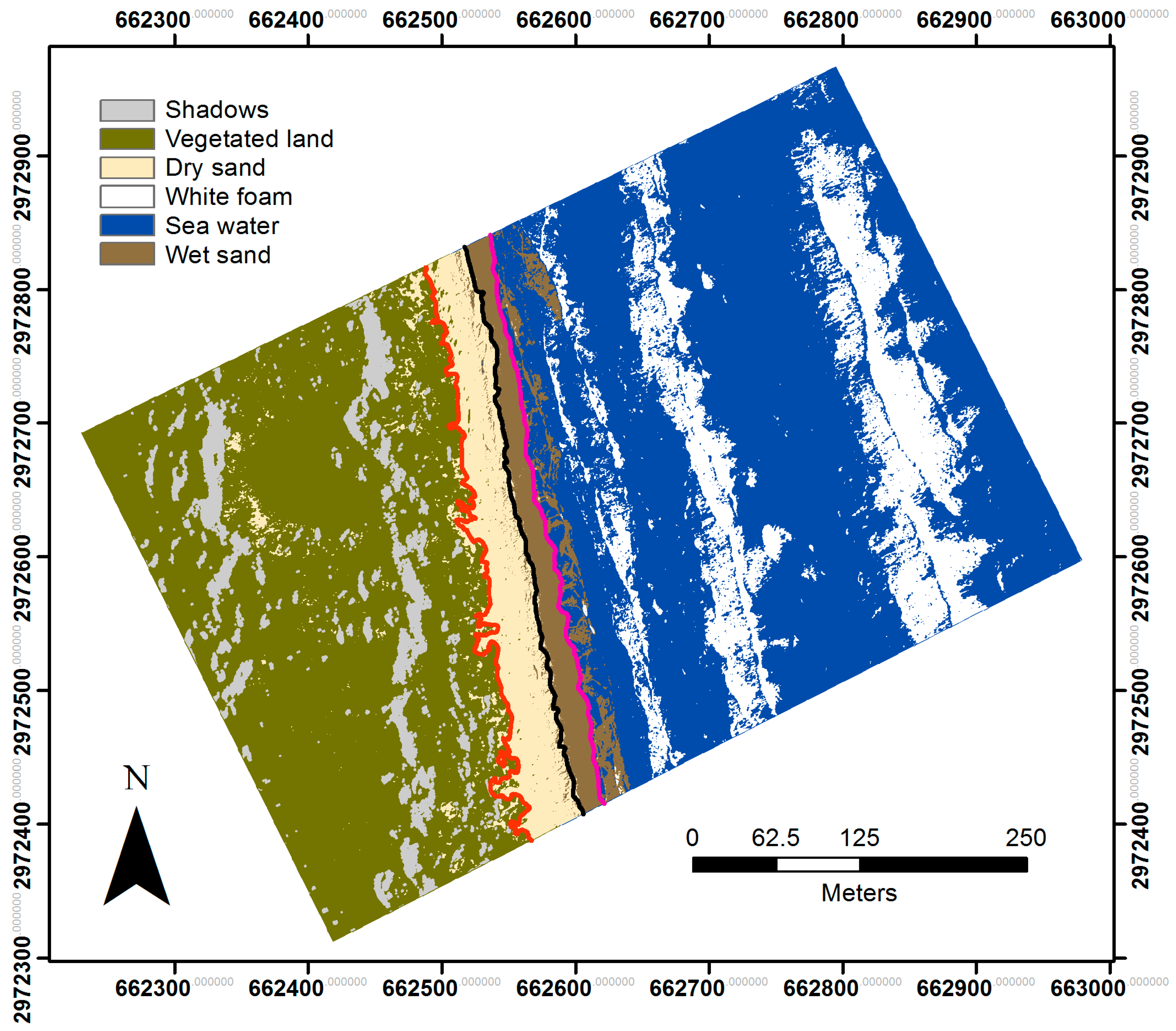
The unsupervised classification map by the red contrast on the 15 × 15 window size (Figure 4) shows that vegetated land can be separated from dry sand clearly and correctly by the three GLCM parameters. Identification of instantaneous water areas is a little unclear. The wet and dry sands can always be separated, however, the boundary location may shift a little bit depending on band and GLCM parameters. The small convex areas of wet sand are filtered out. In Figure 4, the dry sand forms a big contiguous region through the debris spots in the dry sand zone create some fragments, which are typically small and isolated. The instantaneous water line is clearly presented in the landward envelope of the water zone.
As shown in Table 4, the three GLCM textures on the USGS Munsell Value and on the L of CIELUV do not produce better results than those produced using the original RGB band. Except for the L of CIELUV, all other bands obtain the best results at a scale of 1. This is not surprising due to the local property of the LBP. Similar to the GLCM cases, the best accuracy is obtained on the red band.

4.2. Accuracies of Supervised Classification

Based on the results from the unsupervised classification experiments, supervised classifications only use LBP texture at a scale of 1, namely R = 1 and P = 8, and GLCM homogeneity at the red band on 5 window sizes. The results by the RGB bands and three classification methods are displayed in Table 8. The results of LBP and GLCM textures are shown in Table 6 and Table 7, respectively.
For the SVM classification, the two parameters, C and γ, are searched using a 4 × 5 grid of C equal to 1, 10, 100, and 1000, and γ equal to 0.5, 1, 2, 4, and 8. Each combination of parameter choices is checked using 10-fold cross validation, and the parameters with best cross-validation accuracy are selected.
For the RF classification, the number of trees is searched by three orders from one-digit numbers, namely from 3 to 9, two-digit numbers including 11, 21, 31, and 91, and three-digit number including 101, 201, and 90l. The OOB error is convergent when the number of trees is bigger than 301. As a result, 301 was chosen as the number of trees for these classification experiments.
As shown in Table 6, LBP textures do not increase in accuracy for the MLC technique; additionally, they slightly decrease the accuracy for the RF and SVM techniques. Single red band and its GLCM homogeneity cannot reach the same accuracy of RGB bands for the three supervised techniques at the 5 window sizes (Table 7). When red band GLCM homogeneity is added to the three RGB bands, the MLC and the SVM can obtain the same or marginally better results for window sizes less than 31 × 31 pixels; the RF cannot obtain better results.

4.3. Supervised Classification on Photos Using Training Sets from a Different Photo

According to the previous supervised classification experiments, only three original RGB bands are used here. Accuracy of DSC7479 and DSC7611 are listed in Table 8. The results show that training data from one photo can produce approximate accuracies on different photos. The MLC enjoys the most stable performance among the three techniques. The underlying reason may be that the MLC uses statistical characteristics of the training data.
From Table 9, Table 10 and Table 11, it is not surprising that the main confusion is seen in distinguishing between the vegetated land and the dry sand and between the wet sand and the water. There is minor confusion distinguishing between the dry sand, the wet sand, and the water. No misclassifications between the vegetated land and the water were found due to their significant difference in RGB color space. Due to limited space, only error matrices of the MLC on DSC_7559, DSC_7611, and DSC_7479 RGB bands are provided here. The other error matrices are available from the authors upon request.
Our results show that the training data from one photo for classification of another photo is feasible. The site-scale observations are the most effective fields of UAS remote sensing due to their quick turnaround and affordable multiple revisits. The relatively short time for image acquisition is an inherent attribute of site-scale UAS remote sensing. Therefore, no physical barriers exist to hinder using a training dataset from one photo on other photos. The findings also imply that parallel processing of classification is feasible for site-scale UAS remote sensing due to no prerequisite brightness balance.

5. Conclusions

In this paper, the experiments demonstrate the capability of identifying beach zones based on feature textures from UAS hyperspatial RGB imagery through image processing and feasibility of the classification approach. The unsupervised classification can produce meaningful results for further supervised classification analysis. The results show that GLCM and LBP textures can improve slightly the classification accuracy by using both unsupervised and supervised classification techniques for the beach zones. Additionally, the three supervised classification techniques show essentially the same performance. In addition, the experiments indicate that for site-scale UAS remote sensing when we use a training dataset from a photo, we could reach acceptable classification results on different photos.

Acknowledgments

This work was partially supported by the National Natural Science Foundation of China project (41428103) and the National Science Foundation (1429518). Clearly state if you received funds for covering the costs to publish in open access. The UAS data was provided by the TAMU-CC Unmanned Aircraft Systems Program and with the support of the TAMU-CC Lone Star UAS Center of Excellence and Innovation.

Author Contributions

Lihong Su mainly proposed this study and contributed to the experiments, data processing, analysis, and manuscript writing. James Gibeaut mainly contributed to discussion and manuscript revision.

Conflicts of Interest

The authors declare no conflict of interest.

References

  1. Woodroffe, C.D. Coasts: Form, Process and Evolution; Cambridge University Press: Cambridge, UK, 2002; pp. 248–320. [Google Scholar]
  2. Moore, L.J. Shoreline mapping techniques. J. Coast. Res. 2000, 16, 111–124. [Google Scholar]
  3. Addo, K.A.; Walkden, M.; Mills, J.P. Detection, measurement and prediction of shoreline recession in Accra, Ghana. ISPRS J. Photogram. Remote Sens. 2008, 63, 543–558. [Google Scholar] [CrossRef]
  4. Boak, E.H.; Turner, I.L. Shoreline definition and detection: A review. J. Coast. Res. 2005, 21, 688–703. [Google Scholar] [CrossRef]
  5. Texas General Land Office. Texas Coastal Construction Handbook; Texas General Land Office: Austin, TX, USA, 2001; pp. 4–9.
  6. Leatherman, S.P. Shoreline change mapping and management along the U.S. East Coast. J. Coast. Res. 2003, 38, 5–13. [Google Scholar]
  7. Crowell, M.; Leatherman, S.P.; Buckley, M.K. Historical shoreline change: Error analysis and mapping accuracy. J. Coast. Res., 1991, 7, 839–852. [Google Scholar]
  8. Turner, I.L.; Harley, M.D.; Drummond, C.D. UAVs for coastal surveying. Coast. Eng. 2016, 114, 19–24. [Google Scholar] [CrossRef]
  9. Mancini, F.; Dubbini, M.; Gattelli, M.; Stecchi, F.; Fabbri, S.; Gabbianelli, G. Using Unmanned Aerial Vehicles (UAV) for high-resolution reconstruction of topography: The Structure from motion approach on coastal environments. Remote Sens. 2013, 5, 6880–6898. [Google Scholar] [CrossRef] [Green Version]
  10. Long, N.; Millescamps, B.; Guillot, B.; Pouget, F.; Bertin, X. Monitoring the topography of a dynamic tidal inlet using UAV imagery. Remote Sens. 2016. [Google Scholar] [CrossRef] [Green Version]
  11. Gonçalves, J.A.; Henriques, R. UAV photogrammetry for topographic monitoring of coastal areas. ISPRS J. Photogram. Remote Sens. 2015, 104, 101–111. [Google Scholar] [CrossRef]
  12. Brunier, G.; Fleury, J.; Anthony, E.J.; Gardel, A.; Dussouillez, P. Close-range airborne Structure-from-Motion Photogrammetry for high-resolution beach morphometric surveys: Examples from an embayed rotating beach. Geomorphology 2016, 261, 76–88. [Google Scholar] [CrossRef]
  13. Papakonstantinou, A.; Topouzelis, K.; Pavlogeorgatos, G. Coastline zones identification and 3D coastal mapping using UAV spatial data. ISPRS Int. J. GeoInf. 2016. [Google Scholar] [CrossRef]
  14. Husson, E.; Ecke, F.; Reese, H. Comparison of manual mapping and automated object-based image analysis of non-submerged aquatic vegetation from very-high-resolution UAS images. Remote Sens. 2016, 8, 724. [Google Scholar] [CrossRef]
  15. Flynn, K.F.; Chapra, S.C. Remote sensing of submerged aquatic vegetation in a shallow non-turbid river using an unmanned aerial vehicle. Remote Sens. 2014, 6, 12815–12836. [Google Scholar] [CrossRef]
  16. Haralick, R.M.; Shanmugam, K.; Dinstein, I. Textural features for image classification. IEEE Trans. Syst. Man Cybern. 1973, 6, 610–621. [Google Scholar] [CrossRef]
  17. Lillesand, T.; Kiefer, R.W.; Chipman, J. Remote Sensing and Image Interpretation, 6th ed.; John Wiley & Sons: Edison, NJ, USA, 2007. [Google Scholar]
  18. Laliberte, A.S.; Herrick, J.E.; Rango, A.; Winters, C. Acquisition, orthorectification, and object-based classification of Unmanned Aerial Vehicle (UAV) imagery for rangeland monitoring. Photogram. Eng. Remote Sens. 2010, 76, 661–672. [Google Scholar] [CrossRef]
  19. Feng, Q.; Liu, J.; Gong, J. UAV remote sensing for urban vegetation mapping using random forest and texture analysis. Remote Sens. 2015, 7, 1074–1094. [Google Scholar] [CrossRef]
  20. Ojala, T.; Pietikäinen, M.; Mäenpää, T. Multiresolution gray-scale and rotation invariant texture classification with local binary patterns. IEEE Trans. Pattern Anal. Mach. Intell. 2002, 24, 971–987. [Google Scholar] [CrossRef]
  21. Nanni, L.; Lumini, A.; Brahnam, S. Survey on LBP based texture descriptors for image classification. Expert Syst. Appl. 2012, 39, 3634–3641. [Google Scholar] [CrossRef]
  22. Tunnell, J.W., Jr. Geography, climate, and hydrology. In The Laguna Madre of Texas and Tamaulipas; Texas A&M University Press: College Station, TX, USA, 2001; pp. 7–27. [Google Scholar]
  23. Morton, R.A.; McGowen, J.H. Modern Depositional Environments of the Texas Coast; Bureau of Economic Geology, University of Texas: Austin, TX, USA, 1980. [Google Scholar]
  24. Weise, B.R.; White, W.A. Padre Island National Seashore: A Guide to the Geology, Natural Environments, and History of a Texas Barrier Island; Bureau of Economic Geology; University of Texas: Austin, TX, USA, 1980. [Google Scholar]
  25. Morton, R.A.; Speed, F.M. Evaluation of shorelines and legal boundaries controlled by water levels on sandy beaches. J. Coast. Res. 1998, 14, 1373–1384. [Google Scholar]
  26. Ilea, D.E.; Whelan, P.F. Image segmentation based on the integration of colour–texture descriptors—A review. Pattern Recognit. 2011, 44, 2479–2501. [Google Scholar] [CrossRef]
  27. Zhang, H.; Fritts, J.E.; Goldman, S.A. Image segmentation evaluation: A survey of unsupervised methods. Comput. Vis. Image Underst. 2008, 110, 260–280. [Google Scholar] [CrossRef]
  28. Kuehni, R.G. The early development of the Munsell system. Color Res. Appl. 2002, 27, 20–27. [Google Scholar] [CrossRef]
  29. Richards, J.A.; Jia, X. Remote Sensing Digital Image Analysis: An Introduction; Springer: Berlin/Heidelberg, Germany, 2006. [Google Scholar]
  30. Ball, G.H.; Hall, D.J. ISODATA: A Method of Data Analysis and Pattern Classification; Stanford Research Institute: Menlo Park, CA, USA, 1965. [Google Scholar]
  31. Jensen, J.R. Introductory Digital Image Processing: A Remote Sensing Perspective; Pearson Prentice Hall: Upper Saddle River, NJ, USA, 2005. [Google Scholar]
  32. Melgani, F.; Bruzzone, L. Classification of hyperspectral remote sensing images with Support Vector Machines. IEEE Trans. Geosci. Remote Sens. 2004, 42, 1778–1790. [Google Scholar] [CrossRef]
  33. Su, L. Optimizing support vector machine learning for semi-arid vegetation mapping by using clustering analysis. ISPRS J. Photogram. Remote Sens. 2009, 64, 407–413. [Google Scholar] [CrossRef]
  34. Su, L.; Huang, Y. Support Vector Machine (SVM) classification: Comparison of linkage techniques using a clustering–based method for training data selection. GISci. Remote Sens. 2009, 46, 411–423. [Google Scholar] [CrossRef]
  35. Hsu, C.W.; Chang, C.C.; Lin, C.J. A Practical Guide to Support Vector Classification; Technical Report; Department of Computer Science and Information Engineering, National Taiwan University: Taipei, Taiwan, 2009. [Google Scholar]
  36. Ho, T.K. Random decision forests. In Proceedings of the 3rd International Conference on Document Analysis and Recognition, Montreal, QC, Canada, 14–16 August 1995.
  37. Breiman, L. Bagging predictors. Mach. Learn. 1996, 24, 123–140. [Google Scholar] [CrossRef]
  38. James, G.; Witten, D.; Hastie, T.; Tibshirani, R. An Introduction to Statistical Learning; Springer: New York, NY, USA, 2013; pp. 316–321. [Google Scholar]
  39. Rodriguez-Galiano, V.F.; Ghimire, B.; Chica-Olmo, M.; Rigol-Sanchez, J.P. An assessment of the effectiveness of a random forest classifier for land-cover classification. ISPRS J. Photogramm. Remote Sens. 2012, 67, 93–104. [Google Scholar] [CrossRef]
  40. Press, W.H.; Teukolsky, S.A.; Vetterling, W.T.; Flannery, B.P. Numerical Recipes: The Art of Scientific Computing, 3rd ed.; Cambridge University Press: Cambridge, UK, 2007; pp. 840–898. [Google Scholar]
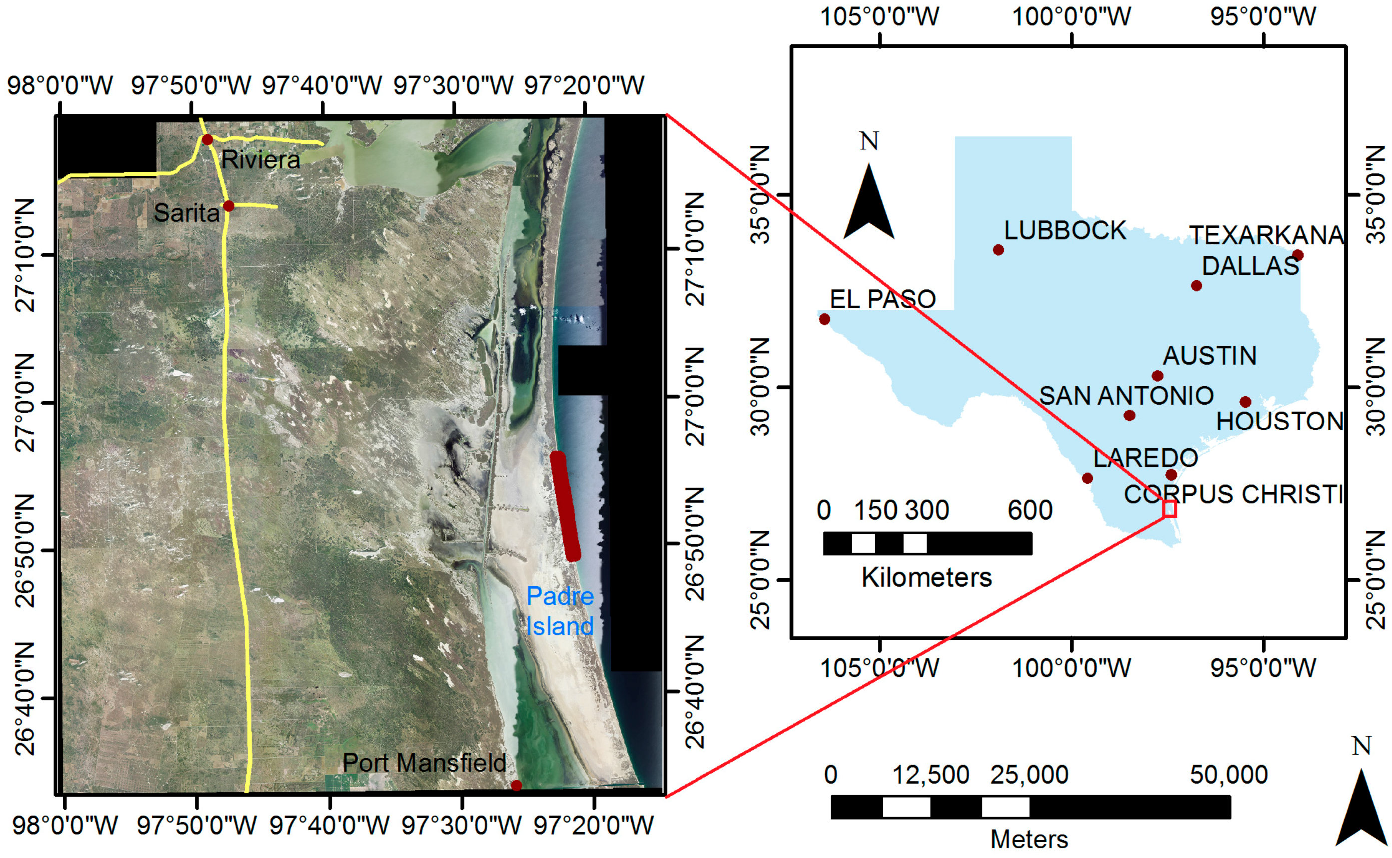
Figure 1. Experiment site at Padre Island in Kenedy County, Texas, USA. The dark red on the left image (geographical extent of Kenedy County) is the area covered by the unmanned aircraft system (UAS) photos.
Remotesensing 09 00159 g001
Figure 2. The 12.9 km coastal area. The (red, green, blue) RGB mosaic image of the 402 photos over the National Land Cover Database 2011 (blue for open water, grey for barren land, and yellow for vegetative cover greater than 20%).
Remotesensing 09 00159 g002
Figure 3. Workflow of the beach zone classification. HSV stands for hue, saturation, and value; USGS is the U. S. Geological Survey; CIELUV stands for the CIE 1976 (L*, u*, v*) color space; GLCM is the gray level co-occurrence matrices; LBP is the local binary pattern.
Remotesensing 09 00159 g003
Figure 4. Comparison of the identified beach zones with manually drawn shorelines on DSC7559 (red for vegetation line, black for wet/dry line, pink for instantaneous water line) by the Universal Transverse Mercator (UTM) zone 14N.
Remotesensing 09 00159 g004
Table 1. Color characteristics of the five objects.
ClassMunsell HueMunsell ValueMunsell Saturation
Vegetated landhighmiddlelow
Sealowmiddlemiddle
Shadowsvery lowlowhigh
White foamvery lowhighhigh
Sand beachhighhighhigh
Table 2. Unsupervised classification accuracy of the original values of the five bands.
BandRedGreenBlueL of CIELUVMunsell Value
Accuracy85.8 (0.81)*82.8 (0.77)81.3 (0.75)82.8 (0.77)83.6 (0.78)
Note: 85.8 (0.81)* means that total accuracy is 85.8% and kappa coefficient is 0.81.
Table 3. Unsupervised classification accuracy of GLCM textures of RGB bands.
Window SizeContrastHomogeneityVariance
RedGreenBlueRedGreenBlueRedGreenBlue
3 × 385.1 (0.80)80.6 (0.74)81.3 (0.75)85.1 (0.80)82.8 (0.77)79.1 (0.72)85.8 (0.81)83.6 (0.78)81.3 (0.75)
7 × 785.8 (0.81)79.9 (0.73)80.6 (0.74)85.8 (0.81)79.9 (0.73)77.6 (0.70)84.3 (0.79)79.1 (0.72)81.3 (0.75)
15 × 1586.6 (0.82)79.9 (0.73)82.8 (0.77)85.8 (0.81)82.1 (0.76)79.1 (0.72)65.7 (0.54)62.7 (0.50)63.4 (0.51)
31 × 3185.6 (0.82)76.1 (0.68)79.1 (0.72)85.1 (0.80)79.9 (0.73)77.6 (0.70)53.0 (0.38)57.5 (0.44)62.7 (0.51)
63 × 6376.1 (0.68)73.1 (0.64)69.4 (0.59)77.6 (0.70)72.4 (0.63)73.1 (0.64)56.0 (0.42)58.2 (0.45)61.2 (0.49)
Table 4. Unsupervised classification accuracy of USGS Munsell HSV and CIELUV color spaces and their GLCM.
Window SizeContrastHomogeneityVariance
Munsell V CIELUV LMunsell VCIELUV LMunsell VCIELUV L
3 × 382.8 (0.77)77.6 (0.70)82.8 (0.77)78.4 (0.71)82.8 (0.77)79.1 (0.72)
7 × 781.3 (0.75)77.6 (0.70)83.6 (0.78)78.4 (0.71)83.6 (0.78)77.6 (0.70)
15 × 1579.9 (0.73)83.6 (0.78)83.6 (0.78)82.8 (0.77)67.9 (0.57)81.3 (0.75)
31 × 3176.9 (0.69)83.6 (0.78)81.3 (0.75)82.8 (0.77)63.4 (0.52)75.4 (0.67)
63 × 6371.6 (0.62)82.8 (0.77)74.6 (0.66)82.8 (0.77)61.9 (0.50)64.2 (0.52)
Table 5. Unsupervised classification accuracy of LBP at three scales.
Scale 1Scale 2Scale 3aScale 3bScale 5
Red87.3 (0.83)85.8 (0.81)82.8 (0.77)82.1 (0.76)67.2 (0.56)
Green82.8 (0.77)81.3 (0.75)78.4 (0.71)78.4 (0.71)70.9 (0.61)
Blue82.1 (0.76)80.6 (0.74)79.1 (0.72)79.1 (0.72)73.1 (0.64)
L of CIELUV82.1 (0.76)83.6 (0.78)82.8 (0.77)82.8 (0.77)82.8 (0.77)
Munsell Value82.8 (0.77)82.1 (0.76)77.6 (0.70)79.1 (0.72)68.7 (0.58)
Table 6. Accuracy of the three supervised classifiers for DSC7559 on the LBP texture. MLC is the maximum likelihood classifications; RF is the Random Forests classifications, SVM is the support vector machines classifications.
Red LBPGreen LBPBlue LBP
MLC92.1(0.89)92.1(0.89)92.1 (0.89)
RF88.6(0.84)88.6(0.84)93.0 (0.90)
SVM89.5(0.85)89.5(0.85)89.5 (0.85)
Table 7. Accuracy of the three supervised classifiers for DSC7559 on the GLCM texture.
Window SizeMLCRFSVMMLCRFSVM
Red GLCM Homogeneity by RedRGB GLCM Homogeneity by Red
3 × 388.6 (0.83)87.7 (0.83)86.8 (0.81)94.7 (0.92)92.1 (0.89)93.9 (0.91)
7 × 786.8 (0.81)88.6 (0.84)89.5 (0.85)93.9 (0.91)93.0 (0.90)94.7 (0.92)
15 × 1590.4 (0.86)90.4 (0.86)91.2 (0.87)92.1 (0.89)92.1 (0.89)93.9 (0.91)
31 × 3189.5 (0.85)89.5 (0.85)92.1 (0.89)93.0 (0.90)89.5 (0.85)94.7 (0.92)
63 × 6388.6 (0.84)89.4 (0.85)91.2 (0.87)92.1 (0.89)90.3 (0.86)92.0 (0.89)
Table 8. Accuracy of the three classifiers for RGB bands on three photos.
DSC_7559DSC_7611DSC_7479
MLC92.1(0.89)94.4(0.92)91.3(0.88)
RF93.0(0.90)89.7(0.85)91.4(0.88)
SVM93.9(0.91)93.5(0.91)91.4(0.88)
Table 9. Error matrix of the MLC on DSC_7559 RGB bands.
VegetatedDryWetWaterRow TotalUser’s Accuracy (%)
Vegetated153001883.3
Dry0330033100.0
Wet001541978.9
Water002424495.5
Column Total15361746
Producer’s Accuracy100.091.788.291.3 92.1
Table 10. Error matrix of the MLC on DSC_7479 RGB bands.
VegetatedDryWetWaterRow TotalUser’s Accuracy (%)
Vegetated353003892.1
Dry324012885.7
Wet00731070.0
Water0004040100.0
Column Total3827744
Producer’s Accuracy92.1%88.9%100.0%90.9% 91.4
Table 11. Error matrix of the MLC on DSC_7611 RGB bands.
VegetatedDryWetWaterRow TotalUser’s Accuracy (%)
Vegetated2800028100.0
Dry025302889.3
Wet0072977.8
Water010414297.6
Column Total28261043
Producer’s Accuracy100.096.270.095.3 94.4