1. Introduction
In Italy, large complex landslides are recurrent phenomena [
1,
2,
3,
4] responsible for destruction of assets and infrastructure, and major economic losses. These phenomena associate a combination of movements, starting as multiple rotational or rotational-translational slides, affecting weak clayey rock masses in the source areas and evolving downhill into an earth slide or flow as the material starts to lose coherence. In the northern flank of the Tuscan-Emilian Apennines (Emilia-Romagna Region, Northern Italy), the Regional Geological Survey has identified more than 70,000 landslides, covering one fifth of the hilly and mountainous territory [
5]. Due to the outcropping lithology, structural setting and geomorphological evolution, about 90% of them are large, ancient earth flows. The majority of these slope movements originated after the Last Glacial Period (approximately from 30,000 BP onwards [
6]), and grew during the Holocene wettest periods through the superimposition of new earth flows. In spite their ancient origin, these phenomena are still very hazardous, alternating long periods of inactivity with sudden reactivations. Long-lasting rainfalls are the most frequent triggering factors during the entire year, while melting of snow cover is particularly effective in the months of March and April, leading to an increase of landslide occurrences and recrudescence [
7]. The reactivation, partial or total, of large earth flows is the main problem the geologists of Emilia Romagna Region have to face nowadays [
8].
The large complex ancient landslides, such as Ca’ Lita [
1,
9,
10,
11], Valoria [
12,
13,
14], Berceto [
15], Corniglio [
16], Roccapitigliana [
17], Ponte Dolo [
18], Lavina di Roncovetro [
19], and Morsiano, Cervarezza, and Signatico [
20], are just few examples of widely investigated instability phenomena following their reactivations in recent times. Some of the performed studies employed ground-based techniques using, for example, seismic [
21] and hydrogeological instruments [
22]. Other studies exploited the contribution of high-resolution DEMs retrieved from photogrammetry and airborne LiDAR [
14] and hyperspectral data [
13]. Rosi et al. [
11] established a wireless sensor network for monitoring purposes. In a few cases InSAR (interferometric synthetic aperture radar) approaches, both ground-based and space-borne [
18], have been used. All of these studies provide data on landslide deformation pattern and style: the movement of most of these landslides is retrogressive on the source areas, advancing in the mid-lower sectors and partially widening on the flanks [
9]. Additionally, information on the variability of the rheological behavior and their pertaining velocities are usually given: in the upper part, the rotational/translational slide evolves with movements of the order of few mm–cm per day while, at the toe, the earth slide/flow moves at velocities of several (tens of) meters per day. The last fifteen years witnessed an increasing number of techniques, applications, and studies aimed at demonstrating the applicability of images acquired by ground-based synthetic aperture Radar (GB-SAR) sensors to continuously monitor ground displacements related to slope instability [
23,
24,
25,
26,
27,
28,
29]. These studies demonstrated the capabilities of the GB-InSAR technique to complement the existing tools for monitoring ground displacements, recording deformation phenomena characterized by a wide range of deformation rates, which roughly range from a few millimeters per year [
26] up to a few meters per day [
30]. Dealing with fast-moving landslides, the time lapse during consecutive SAR acquisitions, a few minutes in most of the available systems can be too long with respect to the velocity of some parts of the investigated scenario. If atmospheric contributions, thermal noises, and other sources of decorrelation are properly corrected [
31,
32], phase ambiguities could occur if the landslide velocity is high (i.e., several meters per day).
To overcome the above-mentioned limitations, and to map deformations induced by fast-moving landslides, a new configuration of the GB-InSAR has been performed, exploiting the high system capability in terms of image acquisition. This paper shows an application of this new acquisition method for the Capriglio landslide, activated in the Tizzano Val Parma municipality (Emilia-Romagna Region, North Italy) after a period of persistent rainfall. Consequently, a continuous surveillance of the landslide dynamic, both in its upper and middle-lower parts, was believed of paramount importance and a prerequisite for providing an early warning of potentially catastrophic displacements. After this event, the Emilia-Romagna Region Civil Protection Department (DPC-RER), responsible for the management of the emergency, appointed the Earth Sciences department of the University of Firenze (DST-UNIFI) to start a GB-InSAR campaign in order: (i) to monitor the landslide kinematics; (ii) to measure the possible ground deformations in correspondence of the urbanized areas and of the landslide toe approaching the Antria bridge in the Bardea Creek; and (iii) to support the local authorities in emergency management. Moreover, aerial optical surveys were performed, to map with high detail the evolution of the area covered by the landslide. Field and GPS surveys were also conducted with the aim of supporting the landslide mapping activities.
In this paper, the results of the GB-InSAR monitoring are presented. The main goal of the GB-InSAR application was the recording of the initial rates of movement, when the landslide could be classified as “moderate” to “rapid”, according to the Cruden and Varnes classification [
33].
The purpose of this paper is two-fold: to show the capability of the employed GB-InSAR system to record the movement of a rapid landslide and to perform long-term and real-time monitoring.
2. The April 2013 Capriglio Landslide Reactivation
2.1. Geologic-Geomorphic Setting
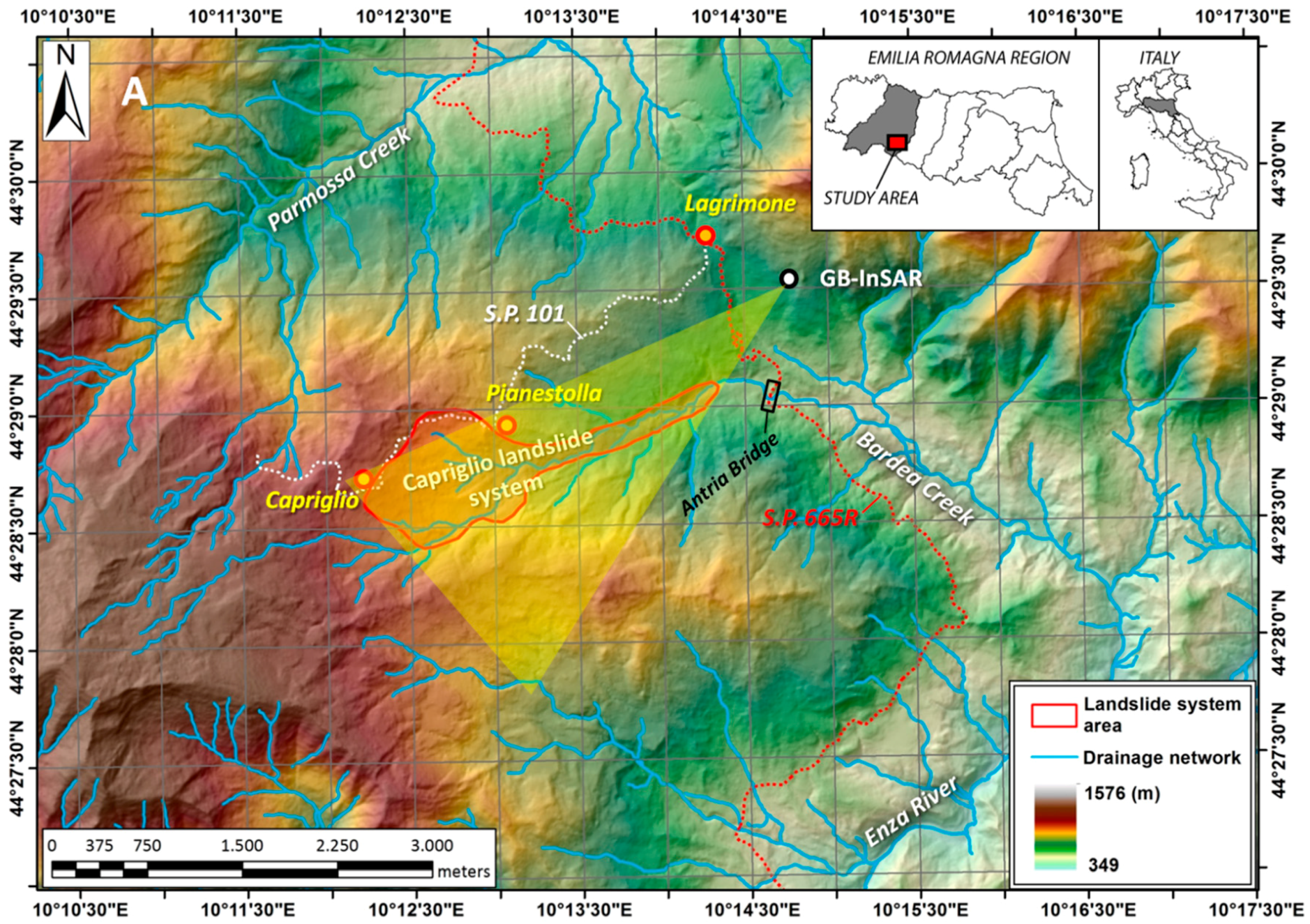
The Capriglio landslide is located in the Northern Apennines within the upper sector of the Enza River basin. The study area is placed within the municipality of Tizzano Val Parma (Province of Parma, Emilia Romagna Region,
Figure 1), about 90 km west of the city of Bologna and about 35 km south-southwest of the city of Parma. In the spring of 2013 the Parma Province was affected by a large number of landslides, as a result of heavy and persistent precipitation (rain and snow), occurring between January and April, and a rapid snow melt in early spring. This resulted in the triggering of about 1400 mapped landslides distributed in over 100 municipalities, causing more than 60 evacuees and severe damages to urbanized areas, infrastructure, and cultivated and pasture lands. In particular, on 6 April 2013, a major event occurred in the Tizzano Val Parma municipality (one of the most severely affected in the whole region), where a large, rapidly moving complex landslide activated. The risk posed by the landslide represented a major concern for local authorities and led to a civil protection emergency.
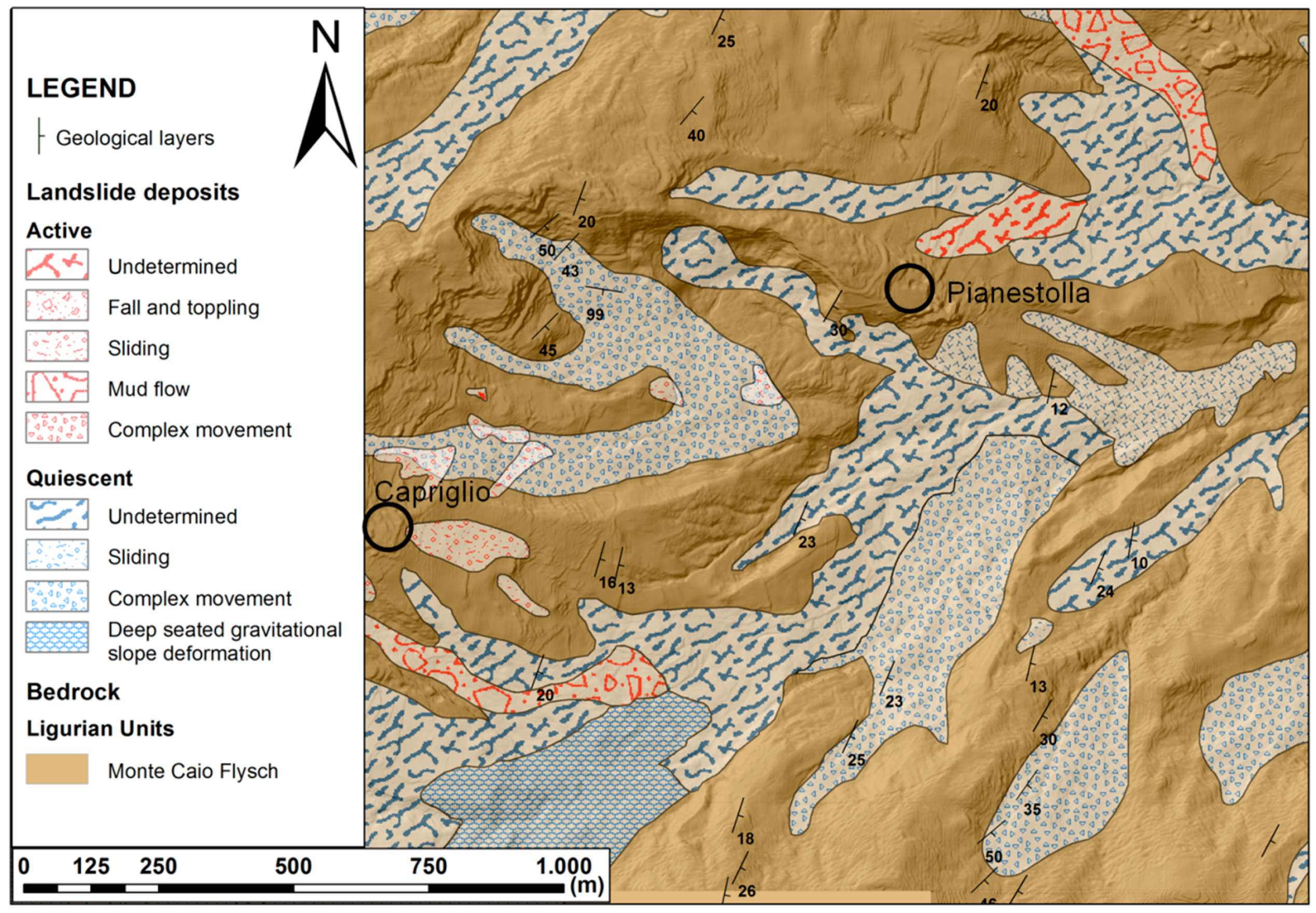
The landslide affected a middle-low mountain area where weak rock masses, constituted by an upper Cretaceous turbiditic deposit (the Mount Caio Flysch, part of the Ligurian Units), extensively outcrops [
34] (
Figure 2). It is formed by thick-bedded calcareous sandy turbidites and marlstones, with a basal clay chaotic complex. In the study area, the Flysch strata dip towards the SE sectors with low to middle angles. In addition to the bedrock, the Capriglio landslide also involved the quaternary cover, mainly represented in the area by smaller pre-existing active and inactive slope movements and related colluviums. In addition to the described event, in situ surveys and available thematic maps indeed highlighted in the study area the presence of many geomorphological features ascribable to pre-existing landslides of different types and ages. Within the Bardea basin, a certain number of instability events can be identified, including complex movements and mud flows. Despite most of these phenomena having been mapped as quiescent, their presence bears witness to the diffuse gravitational instability characterizing the entire basin (
Figure 2).
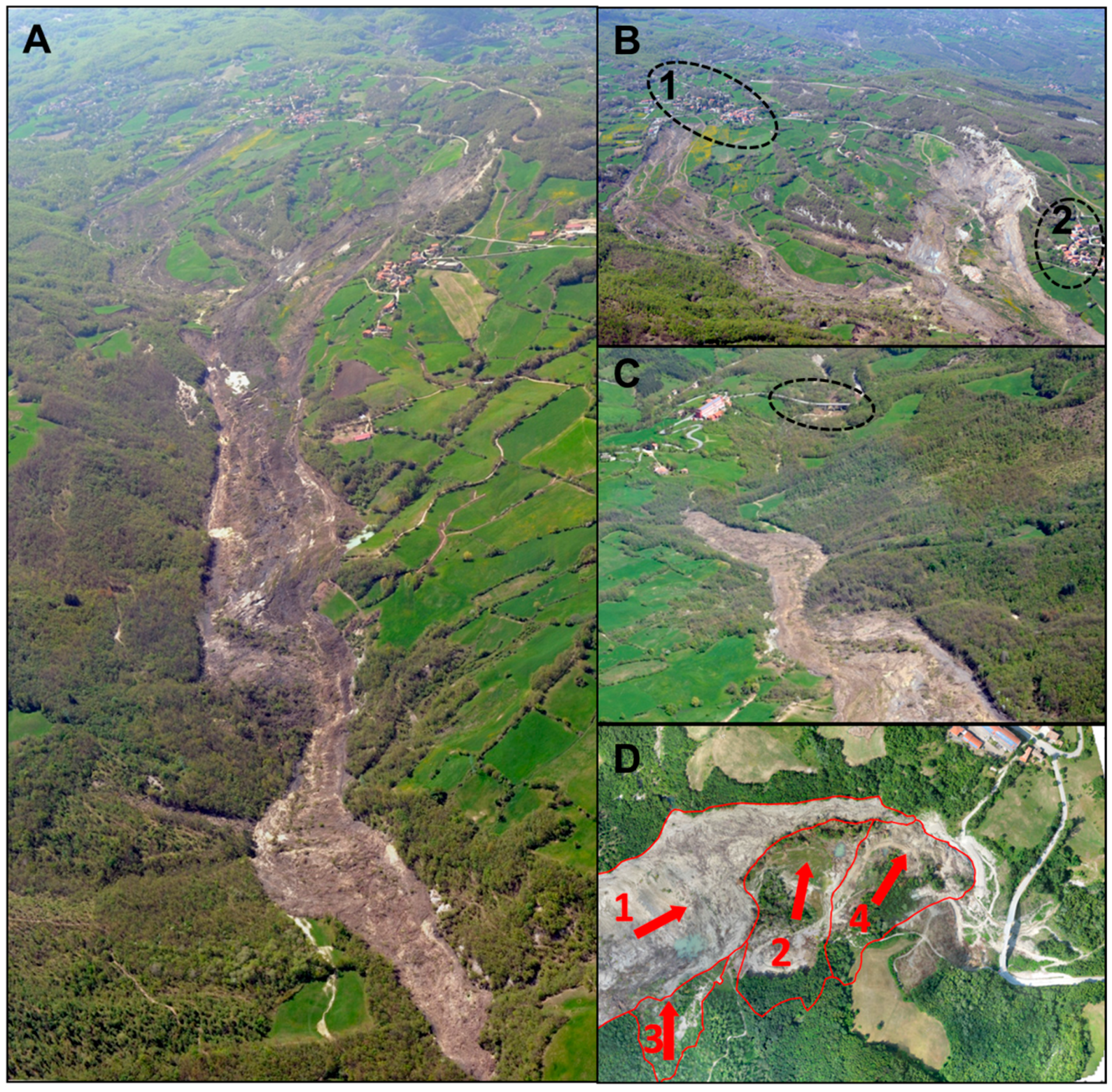
The Capriglio landslide (
Figure 3A) stretches from an altitude of 980 m a.s.l.(above sea level) to about 630 m a.s.l., covering an area of approximately 0.92 km
2 over a length of about 3.6 km, with a travel angle of about 6°. During field surveys, the deposit’s maximum width was measured (about 350 m) and a preliminary estimation of the maximum movement rate was evaluated by observing consecutive landslide toe locations (
Table 1).
The landslide developed on the NE flank of the Caio mountain (1587 m a.s.l.) and channelized within the riverbed of Bardea Creek, a 10-km long left tributary of the Enza River. The landslide area includes mainly cultivated fields, wood, and pasture land and, due to the huge extent and rapid movement, the resulted geomorphological effect was remarkable. It can be considered the largest reactivation landslide documented in the Emilia Romagna Region archives.
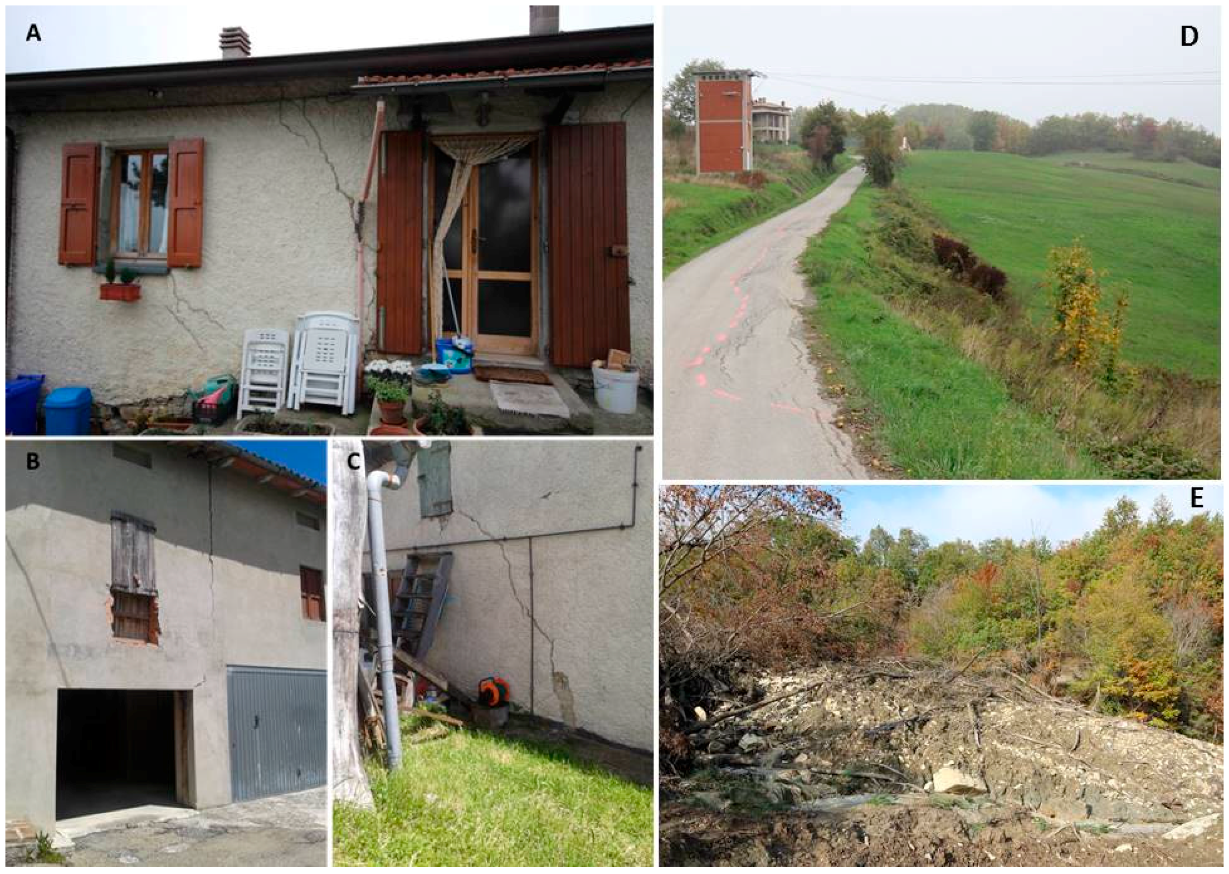
The upper part of the landslide destroyed ca. 450 m of the provincial roadway S.P. 101 and put at high risk the villages of Capriglio and Pianestolla. These two hamlets are located in the upper watershed area of the Bardea Creek and were seriously threatened (directly and indirectly) by potential retrogression of the main scarps. Moreover, the advancement of the toe of the landslide, characterized by a velocity with an order of magnitude of several (tens of) meters per day, represented a real risk for the Antria bridge, located downstream on the Bardea Creek. Such road infrastructure is a transect of the “Massese” provincial roadway (S.P. 665R) and it was considered very strategic for a long time since it was the only local roadway left intact and able to connect the above-mentioned villages, as well as the local economic activities with national sales channels. Fortunately, despite the severity of this event, no fatalities occurred and Capriglio and Pianestolla villages suffered minor damages, though some houses and agricultural warehouse were completely destroyed.
The landslide kinematics included two large adjacent bodies that rapidly activated in sequence, generating some compound landslides, and joined together downstream into a high mobile larger phenomenon. As a whole, such evolving movement can be classified as a roto-translational earth slide with an enlarging activity subsequently evolving in earth flow (complex landslide [
33,
35,
36]). Therefore, it can be considered as a combined system of two large mass movements (
Figure 3B): (i) on 6 April a right bank crown developed downstream of Capriglio village and a landslide started to move as a rotational earth slide, evolving shortly after into a chaotic mass with morphological evidence typical of flows; (ii) on 12 April this landslide activated an area just upstream of the village of Pianestolla, partially characterized by pre-existing instability phenomena, causing an additional translational mechanism (left bank landslide), which affected weathered slope-dipping flysch strata, completely destroying the sector of provincial roadway S.P. 101, and joined into the valley with the first movement, evolving as a large-scale fast earth flow. Morphological evidences in this area and their temporal sequence evolution indicated that the first earth flow determined an unloading of the slope near Pianestolla, inducing the development of a further retrogressive movement, with the rupture surface extending towards the watershed.
The fast superimposition of the collapsed mass on the narrow valley of Bardea Creek determined high availability of water from the main channel and its afferent hydraulic network, which largely permeated within the new chaotic mass, inducing a significant material mobilization. This circumstance resulted in a remarkable advancement of the lower sector of the landslide, which threatened the Antria bridge on the Bardea Creek, located 2 km downstream of Pianestolla (
Figure 3C). In addition, the movement of the landslide toe, though highly mobile, caused a multiple unloading of the right flank of the valley, which, in turn, triggered a series of landslides, further increasing the total volume of the landslide system. These secondary landslides (
Figure 3D), moving NNE (i.e., almost perpendicularly to the main movement direction of the main landslide), partially dammed the Bardea Creek valley and caused a dramatic decrease of the downstream movement of the Capriglio landslide, one hundred meters before the bridge.
The landslide toe evolved with velocities of several tens of meters per day (with peaks of 70–80 m/day) for the first month after the trigger, and of several meters per day (with peaks of 13–14 m/day) from early May to mid-June 2013. These movement rates allowed the phenomenon to be included in the “rapid” and “moderate” classes of the Cruden and Varnes classification [
33].
2.2. Rainfall Leading to Reactivation
The landslide occurred after some weeks of persistent rainfall affecting the area (
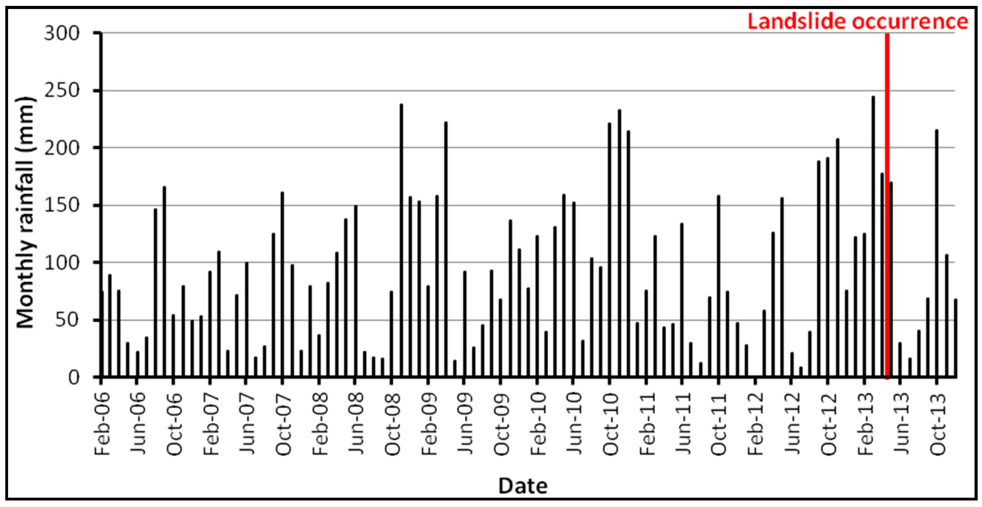
Table 1). Despite the lack of rain gauges close to the landslide, some meteorological stations were available near the area. Hence, the rainfall data recorded at the rain gauge located at Musiara Superiore hamlet have been used. Being located 2.5 km NW of Capriglio, this rain gauge is the closest to the landslide and is installed at an elevation (980 m a.s.l.) similar to the altitude of the crown area of the landslide (982 m a.s.l.). From a climatic point of view, this area of the Apennine range is characterized by an annual average rainfall of about 1000–1200 mm. The highest precipitation levels are recorded in autumn (October–November) and in spring (March–April). The month of July, and secondarily February, are the months with the lowest precipitation. In addition to the rainfall, a main role is played by rapid melting of snow during the spring, as a consequence of the rapid temperature increase at a relatively low altitude.
Analysis of rainfall data of the period 2006–2013 (
Figure 4) allows the identification of intense events in the pluviometric regime before the landslide occurrence, evaluating their role as a trigger. Rainfall data, analyzed month by month, for the 2006–2013 period highlight that February and March 2013, with 125 and 244 mm of cumulated rainfall, respectively, are the wettest months of the analyzed period. It is clear that intense precipitation before the trigger (15-days accumulated rainfall of 180.8 mm) contributed to the increase of the critical state primed by the significant accumulation of rainfall that occurred during January and February, causing the complete saturation of soil and, consequently, the trigger of the landslide.
2.3. Spatio-Temporal Evolution of the Reactivation
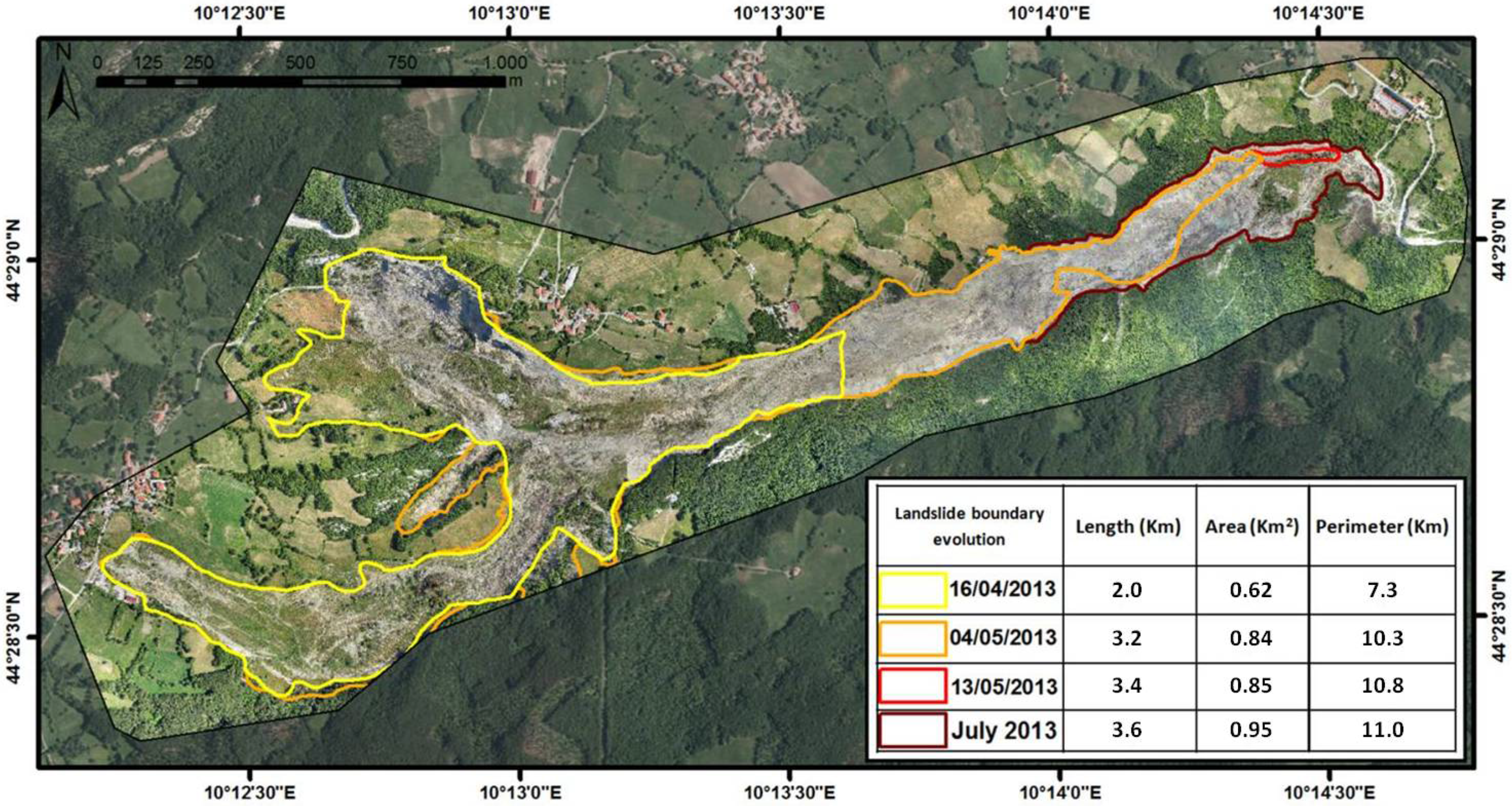
The temporal evolution of the Capriglio landslide system has been mapped (
Figure 5) through the synergic use of aerial and satellite images and GPS surveys [
37,
38]. In particular, the following surveys have been performed:
- On 16 April 2013, a 1.6 m ground resolution Ikonos-2 image was acquired to perform a preliminary landslide boundary assessment. The image was elaborated in rush mode to support emergency response activity of the civil protection in the framework of the Copernicus program of the European Commission.
- On 4 May 2013 an aerial photographic survey was performed in order to acquire high-resolution images of the landslide system and to perform a second preliminary landslide boundary assessment. In order to avoid image geometrical distortions, the cameras were placed in the aircraft hatch in order to obtain a line of sight in a perpendicular direction as much as possible with respect to the topographic surface. The line of flight was aligned along the landslide longitudinal axis at an average altitude of 300 m above ground level, leading to an image geometric resolution of about 20 cm. Other aerial images were also acquired from different lines of sight in order to give a global picture of the landslide. Image overlapping allowed a manual mosaicking and georeferencing in a GIS environment using a previously acquired DEM and aerial optical image of the Emilia Romagna Region as reference base maps.
- On 13 May 2013, a GPS survey of the landslide toe was performed to obtain a further estimation of its location.
- At the end of July 2013 a drone aerial optical survey was performed by Regional Agency for Civil Protection—Emilia Romagna Region, allowing mapping of the final landslide extent.
The landslide boundary assessment allowed us to estimate the multi-temporal evolution of the landslide area, permitting the monitoring of the landslide toe velocity with respect to the reference satellite map acquired on 16 April 2013 (
Figure 5). This helped to estimate the landslide toe velocity in the first two weeks of the post-triggering phase: from about 80 to 15 m/day, corresponding to the “rapid” and “moderate” classes according to the Cruden and Varnes classification [
33]. In addition, it was also shown that, besides the Capriglio and Pianestolla villages, the landslide toe evolution exposed the Antria bridge of the “Massese” 665R provincial road crossing the Bardea Creek to a very high degree of danger.
3. GB-InSAR Methods and Operative Approach
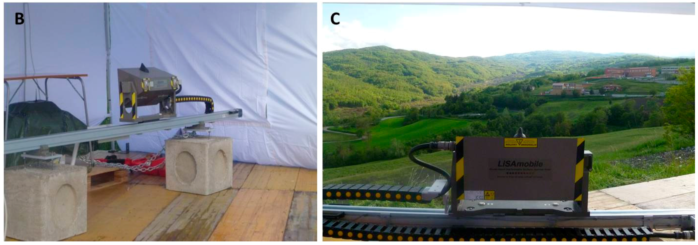
On 23 May 2013, a GB-InSAR system was installed in Lagrimone, a village located on the opposite slope of the Capriglio landslide, in the Tizzano Val Parma municipality (
Figure 6). The objective was the displacement monitoring of the Capriglio landslide toe, as well as the detection of possible millimetric movements affecting Capriglio and Pianestolla villages. The selected location for the installation was revealed to be the best for this purpose. The system employed is a portable SAR device, known as LiSA-Mobile: it is an evolution of the prototypal GB-InSAR instrument, named LiSA (acronym of Linear SAR), developed by the Joint Research Center (JRC) of the European Commission and its spin-off, Ellegi-LiSALab Company [
39,
40,
41]. Beyond the employed technique, there is the exploitation of microwave radiation of the electromagnetic spectrum: by calculating the time that the radiation needs to go from the sensor to a target and back, it is possible to evaluate the distance between the sensor and the target. By comparing successive acquisitions, eventual target displacement, with sub-millimeter precision, can be detected. The comparison is based on the evaluation of the phase difference between the transmitted and the received wave. It is indeed possible to correlate the phase variation with the target displacements: in the same topographic conditions, during subsequent radar acquisitions, the phase shift of the wave mainly depends on occurred target displacements. Phase shift also depends on atmospheric and noise components, which must be properly corrected in order to isolate displacement contributions [
32,
42].
In every radar system, spatial resolution is proportional to the antennas’ length. In ground-based (GB) systems, a suitable resolution requires a physical antenna too large to be practically transported and mounted. To overcome this limit, synthetic aperture radar (SAR) systems have been implemented. SAR is a technique that uses signal processing to improve the resolution beyond the limitation of the physical antenna aperture. In SAR techniques, the motion of a physical antenna along a rail (a few meters long) is used to ”synthesize” a larger antenna. SAR imaging consists of irradiating the targets with a small physical antenna, transmitting a stream of pulses from different positions along the rail. The antennas repeatedly illuminate with successive pulses a specific target to synthesize an aperture that is the same size as the rail length: as the antenna moves, it provides repeated observations of each spot of the scenario. The echo of each pulse is received, recorded, and analyzed [
25,
43,
44,
45,
46,
47]. This allows SAR to achieve high resolution with small physical antennas.
The instrument employed in Tizzano Val Parma is a new generation ground-based system, whose main components are: (i) a 330 cm linear rail (maximum synthetic aperture of 300 cm), along which two antennas that move with millimetric steps to define the synthetic aperture; (ii) a microwave transmitter, that produces, step by step, continuous waves around a center frequency (17.2 GHz); (iii) a receiver that records the amplitude and the phase of the microwave signal backscattered by the target; (iv) the antenna support; (v) a power base, containing a UPS (uninterruptible power supply) to guarantee a constant electrical supply, and boards to increase memory. The system maintains the characteristics of accuracy (sub-millimeter) of a classical LiSA system, but it is implemented with some features which make it easier and faster to install: it has been conceived in a modular configuration with the main components separately arranged, in order to reduce the weight and dimensions of each element. The system is also characterized by higher versatility than the previous instruments, in terms of possible acquisition configurations. A significant advantage is indeed given by the possibility to choose the synthetic aperture length to obtain different SAR configurations, which influences the acquisition time and consequently the detectable velocity. Dealing with a “moderate” to “rapidly” moving landslide, the main limiting factor of the existing systems is the time to acquire a single image, typically ranging from few to several minutes [
24]. In relation to the observed scenario and the velocity of the analyzed displacement, a larger or smaller aperture can be selected to analyze faster or slower velocities. The use of a shorter aperture allows acquiring more data in shorter times, albeit at the expense of spatial resolution and coverage, detecting higher velocities than the typical detectable velocity values. In other words, it determines the acquisition of more interferograms in reduced timespans, but it also implies a reduction in the azimuth resolution, which is inversely correlated to the linear rail length [
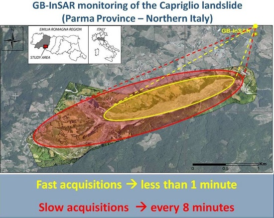
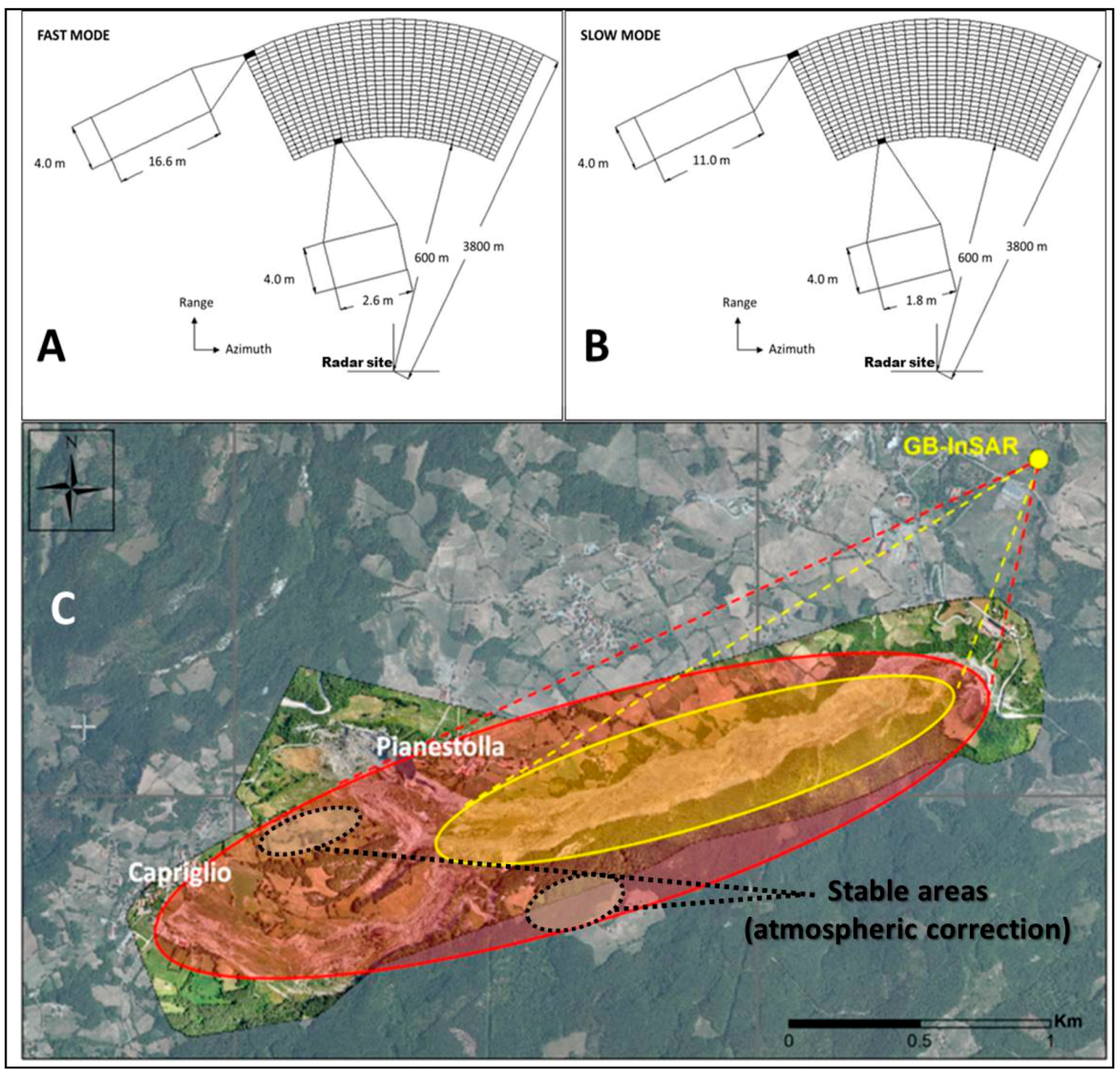
48]. Thanks to this GB-InSAR characteristic, in the early period of the Capriglio landslide monitoring activity, two acquisition modes were arranged: fast and slow (
Figure 6).
Fast mode was performed reducing the linear rail length to 1 m, allowing SAR to detect the whole landslide body, and its high-velocity values, with a reduced azimuth resolution (
Figure 6A–C). Slow mode acquisitions were performed by using the maximum linear rail length (3 m), in order to detect an area that also included the villages of Capriglio and Pianestolla, with acceptable azimuth resolution (
Figure 6B,C). This configuration is more useful to detect lower displacements, eventually affecting buildings/structures. The differences in the detectable areas (
Figure 6) are connected to the needs of compromising between temporal and spatial resolution: the reduction of azimuth resolution in “fast” acquisition mode can be considered acceptable if the acquired data are not so far from the instrument location; therefore, fast acquisitions have been exploited to detect a smaller area (
Figure 6A–C).
Initially, “fast” acquisitions were interchanged with “slow” acquisitions to detect eventual slower displacements affecting Capriglio and Pianestolla villages. During this first period, in order to guarantee a continuous monitoring of the villages, slow mode acquisitions were performed throughout the whole day, suspending them only few minutes a day to perform fast acquisitions. After landslide deceleration, only slow mode acquisitions were performed until December 2014.
Some difficulties partially limited the GB-InSAR application on the presented test site: (i) the widespread vegetation cover, which in some measure reduced the observable scenario (low coherence of the radar signal [
49]), but that, fortunately, did not affect the landslide body and the villages; (ii) the high distance between the radar location and the study area, which determined a reduced azimuth resolution in correspondence with the farthest portion of the scenario, and which implies a very high variation of the atmospheric contribution on the whole scenario; and (iii) the intrinsic GB-InSAR feature to be able to detect only the component of the displacement vector which is parallel to the instrument line of sight (LOS), which implied an underestimation of the detected displacements in specific sectors of the study area (mainly located near the village of Pianestolla, where the movement direction is nearly perpendicular to the radar LOS (about 35% of the estimated real displacement).
Proper atmospheric correction has been applied to radar images, in order to reduce the related decorrelation effect. The atmospheric delay is a function of changes in the refractive index, which depends on temperature, humidity, and pressure differences. As the investigated scenario is affected by oscillation of these parameters, a proper correction is crucial in order to accurately interpret radar data. The relation between path delay and atmospheric parameters has been determined under the assumption of a uniform atmosphere (constant atmospheric parameters). Specifically, the atmospheric delay has been estimated on stable areas, where the phase of the radar signal only depends on the atmospheric component and random noise, following the approach proposed by [
31] and [
32]; these areas have also been selected on the basis of high coherence values of the radar signal (
Figure 6C). The atmospheric component is identified in the spatial low frequency component of the phase shift. Assuming a linear relation between the effect of the atmosphere and the distance instrument-target, the range variation of the atmospheric delay has been interpolated for the whole length of the detected scenario.
5. Discussion
Following the landslide trigger on 6 April 2013, the Capriglio and Pianestolla villages suffered only minor damages and the landslide, evolved from two main earth slides close to them into a rapidly moving earth flow, deeply channelized within the Bardea Creek riverbed. Following the event, the emergency management activities focused primarily on the two villages exposed to the risk of potential retrogression of the main landslide scarps.
Since the end of April 2013, the lower part of the landslide also drew the attention of the involved authorities, as the 5 May 2013 aerial survey revealed that the entire landslide toe was moving rapidly along the Bardea Creek with respect to the reference satellite images of 16 April 2013, for a total of more than one kilometer with a mean rate of several dozens of meters per day. In this emergency framework, the installation of a monitoring system was extremely necessary. To guarantee a constant (24/7) stream of information, a GB-InSAR system was installed. According to [
9], the most serious gap for the extensive use of GB-InSAR devices as operational monitoring tools was the limited range of recordable velocities, which limits the applicability of InSAR approaches only to slow-moving landslides, excluding fast-moving phenomena. In this context, the complex dynamics of the Capriglio landslide has generated a challenging situation to face with a GB-InSAR system. In addition to the landslide size and velocity, the difficulties also consisted of the different deformation pattern and in the widespread vegetation cover within the observed scenario, with the exception of the well-exposed landslide mass and the two villages, located 2.8 and 3.8 km from the radar instrument, respectively. Fast mass movements, like the studied one, are difficult to be monitored by means of the ground-based InSAR approach. In the field of interferometry, the range of observable motions is governed by the refresh time (i.e., the elapsed time between the acquisitions of two consecutive images), which, in turn, depends on the acquisition time (time necessary to collect the radar signal of a single SAR image) [
50], typically in the order of few minutes for the existing operational devices. To avoid ambiguity problems and to correctly retrieve the actual velocity, the displacement of the observed target should be contained within ±
λ/4 between two consecutive SAR acquisitions. When the investigated landslide velocity exceeds the observable one, the only viable approach is to reduce the synthetic aperture to decrease the acquisition time, with a consequent coarsening of the spatial resolution and decrease of the covered area. When dealing with landslides (such as the Capriglio one) associating different deformation patterns, the only viable approach is to acquire images with different synthetic apertures, exploiting the versatility of the GB-InSAR system in terms of images acquisition. To cope with the scenario generated by the Capriglio landslide, the alternation between fast and slow acquisitions has been the approach designed to retrieve useful information about distinct displacement regimes, ranging from small to high deformation rates.
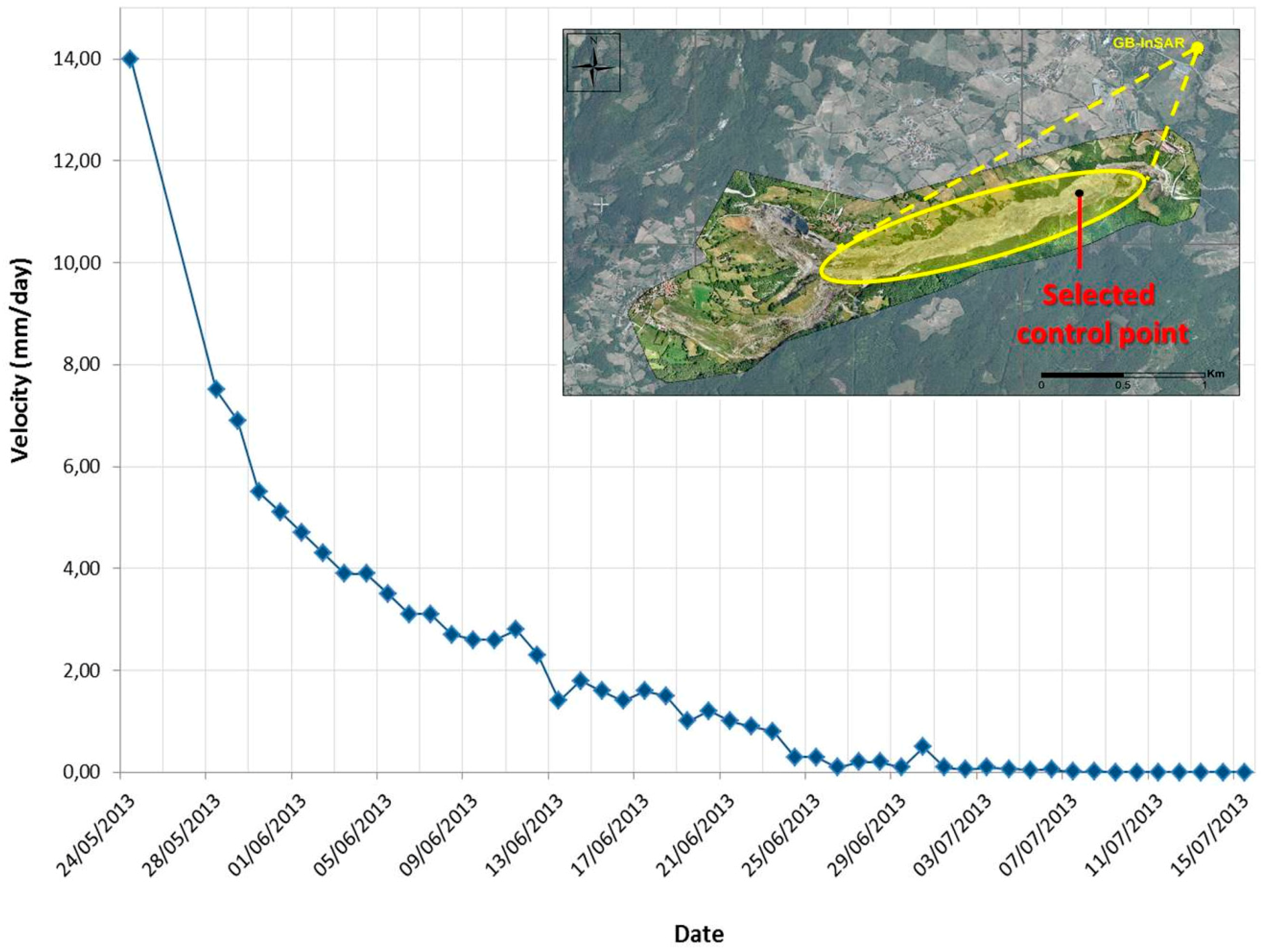
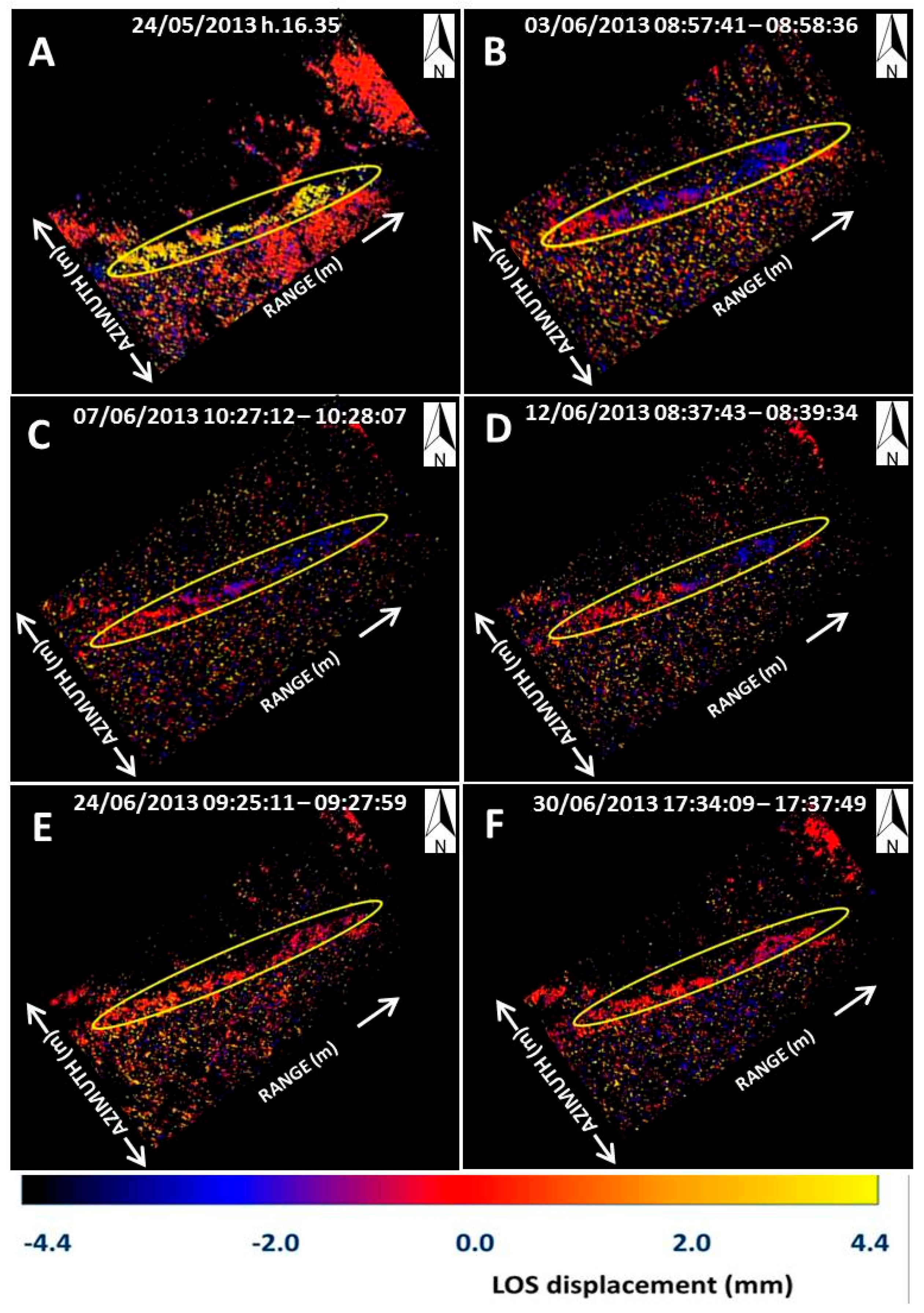
The “fast acquisition” mode, exploited during the first weeks of monitoring, provided very important information on the rate of movements of the landslide lower sector. This configuration allowed the measurement of the velocity on the order of several meters per day (with a peak of 14 m/day), overcoming the previously set threshold of about 3 m/day, obtained by using similar instruments [
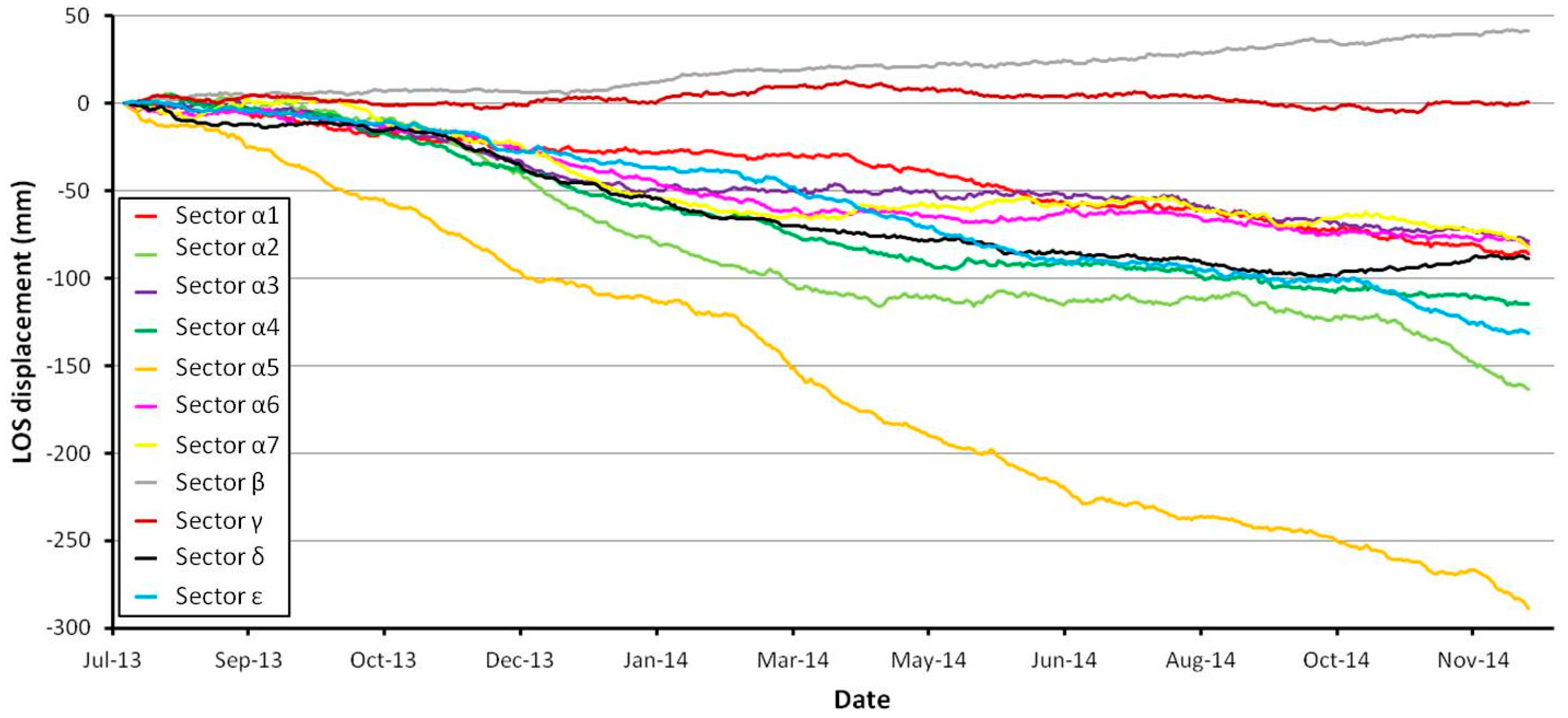
24]. This configuration successfully supported the daily emergency management posed by the rapid advancing landslide’s toe, which seriously threatened the Antria bridge on the Bardea Creek. Two months after the beginning of the monitoring activities, displacement velocities in the landslide body had decreased to a lower level (
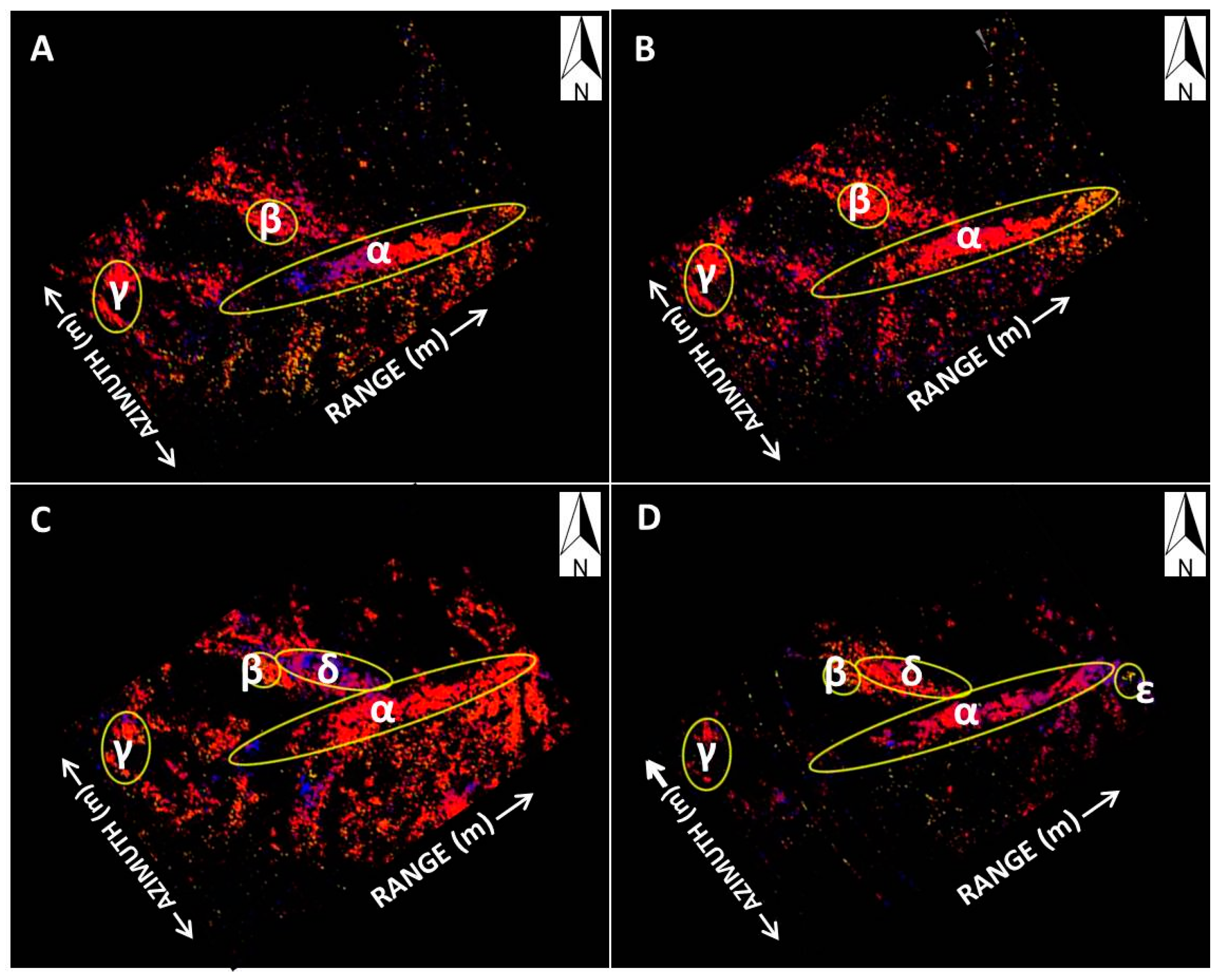
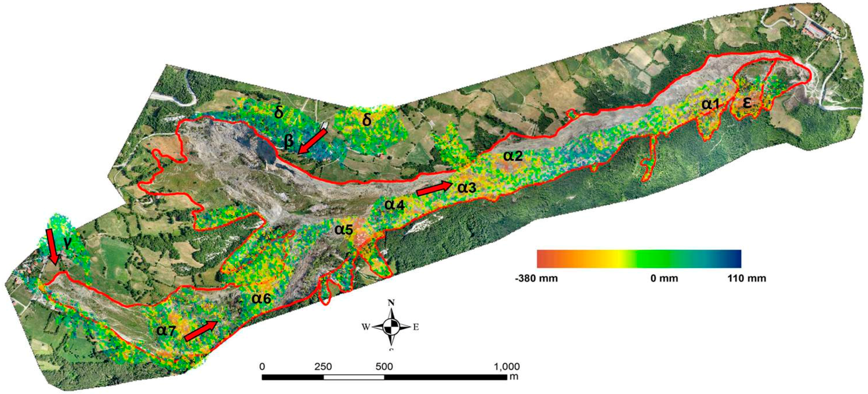
Figure 8). Hence, the “slow acquisition” mode became ordinary. The slow acquisition mode, characterized by wider coverage and finer resolution, has provided long-term information (17 July 2013 to 31 December 2014) and a synoptic view of the deformation processes affecting the Capriglio landslide area. The greatest benefit of this mode was the possibility to retrieve the minor, short-term deformation affecting the village of Pianestolla (sector B in
Figure 10) and to assess the substantial stability of the Capriglio village (sector γ in
Figure 10).
The high temporal acquisition frequency, the fine ground cell resolution, and the capacity to detect simultaneously both rapid movement and millimetric deformation, makes the GB-InSAR device, coupled with mapping and field surveys, an instrument of great relevance in the field of landslide-related risk management.
6. Conclusions
This paper presents the main findings of the long-term, real-time monitoring of the Capriglio landslide in the Emilian Apennines (Northern Italy). The landslide, which occurred on 6 April 2013, after a period of prolonged rainfall, presents complex features as it started as a roto-translational earth slide and evolved into an earth flow, which channelized in the Bardea Creek riverbed, to form a large scale, rapidly moving earth flow. The landslide reached a total length of about 3.6 km, with a volume of about 3,600,000 m3.
Through the integrated use of aerial, satellite, and drone images and GPS surveys, the temporal evolution of the Capriglio landslide system was mapped, permitting the preliminarily assessment of the landslide toe evolution and velocity with respect to the reference satellite map acquired on 16 April 2013 (
Figure 5). This led to the first estimation of the landslide toe velocity immediately after the trigger, ranging between 80 to 15 m/day, corresponding to the "rapid" and "moderate" classes according to the Cruden and Varnes (1996) classification [
33].
Since this landslide exhibited a complex displacement pattern, we exploited the versatility and flexibility of a ground-based interferometric system to guarantee a constant (24/7) stream of information on the evolution of the landslide. This approach, based on the alternation of slow and fast acquisitions, allowed to detect and measure both the minor deformation affecting the areas of Capriglio and Pianestolla villages in the upper part of the landslide, and the remarkable displacement rate of the rapid-to-moderate advancing landslide toe, threatening the strategic Antria bridge, straddling downstream the Bardea Creek.
The rationale underpinning the proposed approach is that a landslide, depending on its extension and kinematics, may require different, but simultaneous, forms of analysis for a proper investigation. When dealing with complex phenomena, like the Capriglio landslide, the fundamental aspect is the design of integrated analyses, encompassing continuous monitoring information (like those provided by SAR images), traditional instruments (e.g., GPS), remote sensing data (like those provided by satellite/aerial/drone), and field investigations. The synergistic use of these techniques provides a wide range of information and is strategic for landslide analysis in operational scenarios.


 ,
, 


