Article

Leveraging Multi-Sensor Time Series Datasets to Map Short- and Long-Term Tropical Forest Disturbances in the Colombian Andes

by
Paulo J. Murillo-Sandoval
1,2,*,
Jamon Van Den Hoek
3 and
Thomas Hilker
1,4
1
Department of Forest Engineering, Resources and Management, Oregon State University, Corvallis, OR 97331, USA
2
Departamento de Topografía, Facultad de Tecnologías, Universidad del Tolima, Ibagué 73000 6299, Colombia
3
College of Earth, Ocean and Atmospheric Sciences, Oregon State University, Corvallis, OR 97331, USA
4
Deceased
*
Author to whom correspondence should be addressed.
Remote Sens. 2017, 9(2), 179; https://doi.org/10.3390/rs9020179
Submission received: 24 December 2016 / Revised: 13 February 2017 / Accepted: 15 February 2017 / Published: 21 February 2017

Abstract

:
The spatial distribution of disturbances in Andean tropical forests and protected areas has commonly been calculated using bi or tri-temporal analysis because of persistent cloud cover and complex topography. Long-term trends of vegetative decline (browning) or improvement (greening) have thus not been evaluated despite their importance for assessing conservation strategy implementation in regions where field-based monitoring by environmental authorities is limited. Using Colombia’s Cordillera de los Picachos National Natural Park as a case study, we provide a temporally rigorous assessment of regional vegetation change from 2001–2015 with two remote sensing-based approaches using the Breaks For Additive Season and Trend (BFAST) algorithm. First, we measured long-term vegetation trends using a Moderate Resolution Imaging Spectroradiometer (MODIS)-based Multi-Angle Implementation of Atmospheric Correction (MAIAC) time series, and, second, we mapped short-term disturbances using all available Landsat images. MAIAC-derived trends indicate a net greening in 6% of the park, but in the surrounding 10 km area outside of the park, a net browning trend prevails at 2.5%. We also identified a 12,500 ha area within Picachos (4% of the park’s total area) that has shown at least 13 years of consecutive browning, a result that was corroborated with our Landsat-based approach that recorded a 12,642 ha (±1440 ha) area of disturbed forest within the park. Landsat vegetation disturbance results had user’s and producer’s accuracies of 0.95 ± 0.02 and 0.83 ± 0.18, respectively, and 75% of Landsat-detected dates of disturbance events were accurate within ±6 months. This study provides new insights into the contribution of short-term disturbance to long-term trends of vegetation change, and offers an unprecedented perspective on the distribution of small-scale disturbances over a 15-year period in one of the most inaccessible national parks in the Andes.

Graphical Abstract

1. Introduction

Protected areas are vital for preserving the planet’s biodiversity and maintaining functional terrestrial and aquatic ecosystems [1]. The tropical Andes, in particular, are a “hyper” hotspot for endemism and conservation support [2]. However, protected areas in the Colombian tropical Andes are under threat from anthropogenic land uses such as cattle grazing, agriculture and population migration [3,4,5,6,7], which have led to deforestation and degradation of protected landscapes [8]. Monitoring long-term ecological processes in these protected areas is therefore crucial to ecological conservation and biodiversity [9]. While remote sensing presents the ideal means to frequently and regularly characterize vegetation change over large and remote areas without the need for physical access, remote sensing of the Colombian Andes is challenging due to frequent cloud cover, complex topography, and regional insecurity (e.g., armed conflict) that impede field validation. Indeed, to date, most studies on Latin American tropical forests have been confined to the Amazon basin’s lowlands rather than the Andes region [10,11].
In the Andes, as well as other mountainous regions, studies of vegetation dynamics have typically used bi- or tri-temporal satellite images acquired on relatively cloud-free dates [11,12,13]. Such temporally coarse and irregular change assessments are prone to confusing seasonal (intra-annual) vegetation dynamics with inter-annual changes [14,15] and are wholly dependent on the quality of images selected for analysis [16]. In Colombia, the ecological monitoring of protected areas is managed by Colombian National Natural Parks (Parques Nacionales Naturales), and based on maps generated every five years using the Corine Land Cover inventory (CLC), which is partially or poorly validated in many remote areas [17,18]. Such simplistic representations of vegetation change are unable to capture the complex co-evolution of natural and social systems across different spatial and temporal scales.
In an effort to provide a more systematic perspective of vegetation dynamics and illuminate spatially detailed patterns, we employ a multi-scale time series assessment of forest disturbance over Picachos National Park and its surrounding area from 2001–2015 using two datasets: the Moderate Resolution Imaging Spectroradiometer (MODIS)-based Multiangle Implementation of Atmospheric Correction (MAIAC) time series, and the Landsat archive from 1996–2015 (Landsat 5, 7, and 8). MAIAC is a relatively new cloud screening and atmospheric correction technique that provides a more complete description of the physical system under investigation and overcomes many restrictions faced by conventional satellite retrievals (e.g., assumed Lambertian reflectance), especially in tropical regions [19,20]. MAIAC provides a more confident interpretation of vegetation trends with much greater temporal fidelity than what could be achieved with a bi or tri-temporal comparison [21,22], but its coarse spatial resolution does not support detection of fine-scale changes. The Landsat archive, with its 30 m spatial resolution and 16-day revisit period, is more suitable for monitoring small-scale processes of deforestation and degradation [23,24] like those present in Picachos and other regions of montane in Colombia [11].
To characterize time series trajectories and trends, we apply the Breaks For Additive Season and Trend (BFAST) algorithm, which has successfully been used to detect forest cover changes in tropical forests with comparable structure to Picachos [14,25]. BFAST was selected over other well-known disturbance monitoring algorithms such as LandTrendr [26] and Vegetation Change Tracker (VCT) [27] for two main reasons. First, BFAST has been shown to be more resilient to noise and missing data (i.e., low data availability or cloud cover) [14,25,28,29,30]. Second, BFAST produces sub-annual information on disturbances and trends rather than the annual scale of LandTrendr and VCT [27,31]. Two different implementations of BFAST were applied: we first used the dense MAIAC time series to quantify multi-year vegetation greening and browning trends and recorded breakpoint dates, which may indicate disturbance or a significant deviation in vegetation trends [32]. Second, we used the BFAST Monitor method and all available Landsat imagery to identify annual disturbances [14], which were independently validated using TimeSync [31]. Short-term Landsat disturbances were then used to validate the timing and distribution of longer-term MAIAC trends. Collectively, these techniques present an effective and scalable framework for monitoring short- and long-term vegetation disturbances and trends in the Andes and other mountainous forested regions.

2. Materials and Methods
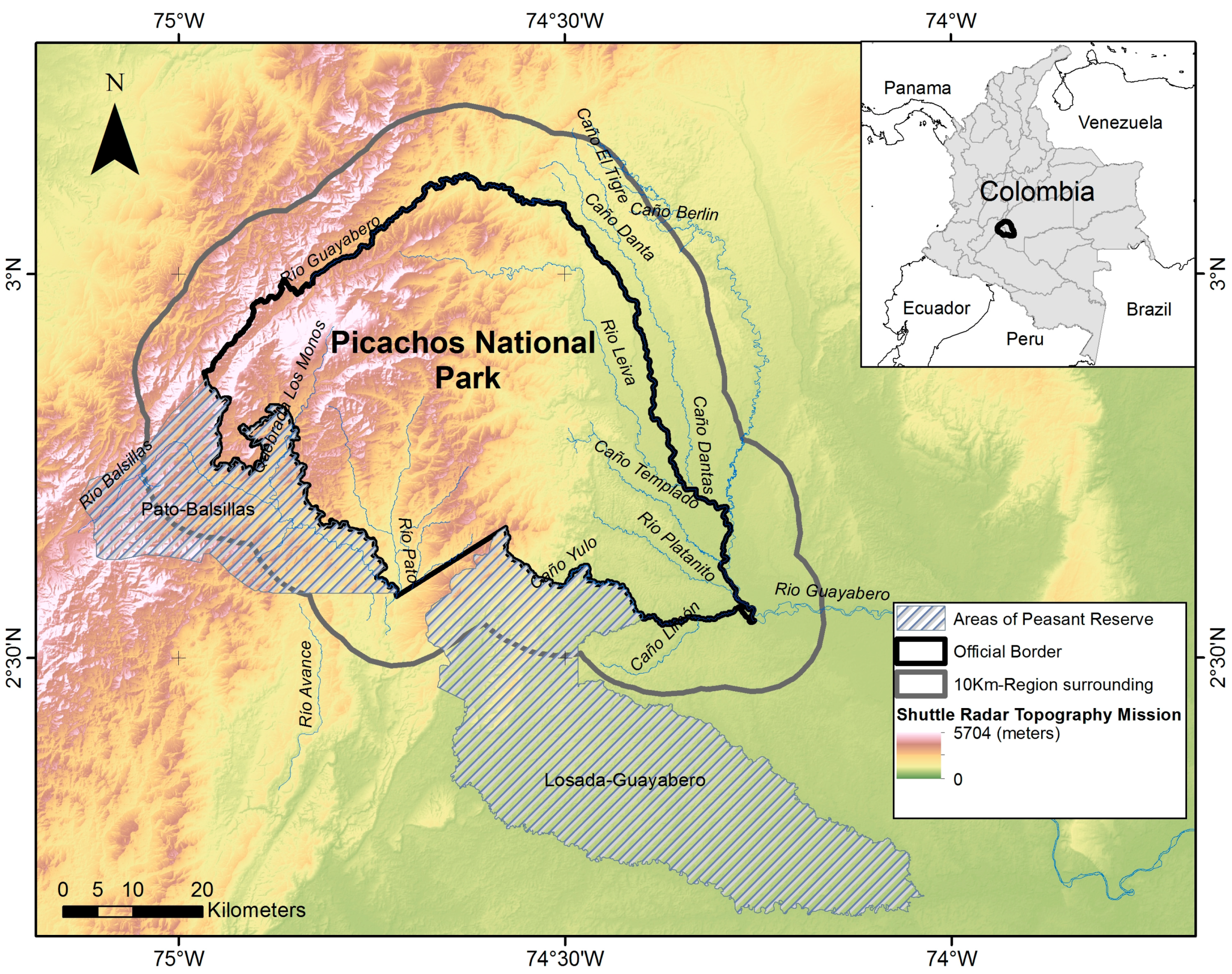
2.1. Study Area

Picachos National Park was established in 1977 and is the third largest national park in the Colombian Andes with an area of approximately 288,000 ha. It has a pronounced elevation gradient spanning 450–3800 m, and is characterized by high annual rainfall (4000 mm/year) and a diverse mosaic of tropical ecosystems (Figure 1). Picachos also has great hydrological importance, as rivers with headwaters in the park feed the basins of the Orinoco and Amazon rivers. While Picachos is a Category II Park as designated by the International Union for Natural Conservation with the stated goal of conserving large-scale ecological processes, species, and ecosystems for current and future generations [33], more than 200 families—many fleeing armed conflict—have settled in the park over the last 25 years [34] and introduced novel land uses such as cattle grazing and subsistence agricultural production, including illicit coca cultivation [35]. Moreover, during the early 2000s, the surroundings of Picachos were legally sited by FARC–EP (Fuerzas Armadas Revolucionarias de Colombia–Ejercito del Pueblo) as part of a negotiation process conducted by the former Colombian government. This agreement collapsed, and the conflict intensified from 2002 to 2010. In recognition of these cross-border processes, our study area includes Picachos as well as the 10 km region surrounding the park.

2.2. MAIAC Data

The MODIS sensor is a pillar of large-scale remote sensing studies due to its superior data quality and daily global coverage [36]. MODIS surface reflectance is regularly derived from top of atmosphere measurements using pixel-based atmospheric correction and cloud screening [37]. Nevertheless, errors in the estimation of atmospheric aerosol loadings [38,39,40] and deficiencies in cloud screening [19] introduce variability in estimated surface parameters unrelated to actual changes in land cover [41], and this may lead to incorrect quantification of vegetation trends [39].
As an alternative to conventional MODIS at-surface products, the Multi-Angle Implementation of Atmospheric Correction (MAIAC) is a novel cloud-screening technique that enhances land surface reflectance based on MODIS C6 Level 1B data [21]. MAIAC’s cloud detection technique yields a noise reduction by a factor of 3–10 compared to standard MODIS surface reflectance products (MYD09, MYD09GA) and derived composites (MYD09A1, MCD43A4, and MYD13A2-Vegetation Index) without the conventional assumption of Lambertian land surface behavior [19,20]. The improvements offered by MAIAC increase the number of viable clear-sky observations by a factor of 2–5 [19], which is especially valuable for monitoring vegetation dynamics in the persistently clouded tropics [42,43]. We used 8-day composite Normalized Difference Vegetation Index (NDVI) observations at 1-km resolution from January 2001 to June 2014 as input for the BFAST analysis.

2.3. MAIAC-Based Trend Detection with BFAST

BFAST iteratively decomposes time series data into trend, seasonal and noise components and supports detection of structural changes (i.e., breakpoints) in both trend (i.e., browning or greening) and seasonal components [44,45]. The parametrization of BFAST is based on a single parameter, h, the inverse of which identifies the largest number of breakpoints that could be detected in a given time series [46]. We set h = 0.15 to reduce the influence of persistent cloud cover that introduces missing data into the MAIAC-NDVI time series. With our MAIAC-NDVI time series being 13.5 years in duration, h = 0.15 means we would have a minimum segment length of at least 2.03 years (93 observations) between breakpoints.
We evaluated the ecological significance of each segment’s slope (β) output by BFAST (Figure 2). The trend within each segment is assumed to be linear and is estimated using robust linear regression [45]. Only segments with significant β values (i.e., non-zero trends) were considered to be potential greening (positive slope) or browning (negative slope) segments, and were tested against the null hypothesis of β = 0 at α = 0.05. At each pixel, the total respective durations of greening and browning periods were calculated as the sum of individual segments with significant slopes. All analyses based on MAIAC were performed in R using the greenbrown library [47].

2.4. Landsat Imagery

We used all available Level-1 Terrain-Corrected (L1T) surface reflectance-corrected Landsat images from path/row 8/58, which covers Picachos in its entirety. In total, this amounted to 374 Landsat 5, 7 and 8 images from 1996–2015; images with over 50% cloud cover were removed, leaving 149 Landsat images for the analysis (Table S1, Figure S1). Cloud masks produced using Landsat Ecosystem Disturbance Adaptive Processing System (LEDAPS), [48], Function of Mask (FMask) [49], and Landsat 8 Surface Reflectance (L8SR) algorithms [50,51] were applied, and NDVI was calculated for all images. Although other vegetation indices have shown less sensitivity to saturation issues in tropical forests, recent studies have demonstrated that NDVI is less affected by sun-sensor geometry variation [20,52] as well as variation in the frequency distribution of observations [29], both of which are relevant for time series analysis. The cross calibration between Thematic Mapper (TM), and Enhanced Thematic Mapper Plus (ETM+) sensors supports a continuity of cross-sensor NDVI trends during the study period [50,53,54]. However, TM/ETM+ and Landsat 8 Operational Land Imager (OLI) do not offer such consistency. Zhu et al. [50] found that OLI-derived NDVI values were positively biased with respect to ETM+ by about 0.04. Consequently, we transformed NDVI surface reflectance-corrected data using the methods described by Roy et al. [55] to minimize OLI’s positive bias and ensure NDVI consistency across Landsat sensors.
To simplify image processing, a forest/non-forest mask was applied to the Landsat archive by masking out all pixels with less than 50% tree cover from the “Year 2000 forest cover” data product by Hansen et al. [56]. We also removed pixels labeled as “rainfed cropland” according to the Land Cover V 2.5 product based on 1 km SPOT-VEGETATION and 300 m Medium Resolution Imaging Spectrometer (MERIS) data with the epoch centered on 2000 (1998–2002) [57]. Following recommendations by Hamunyela et al. [28], we also masked pixels with less than 30 observations (20% of the full time series) and less than 7 observations in the historical period (1996–2000) (see Section 2.5 and Figure 3).

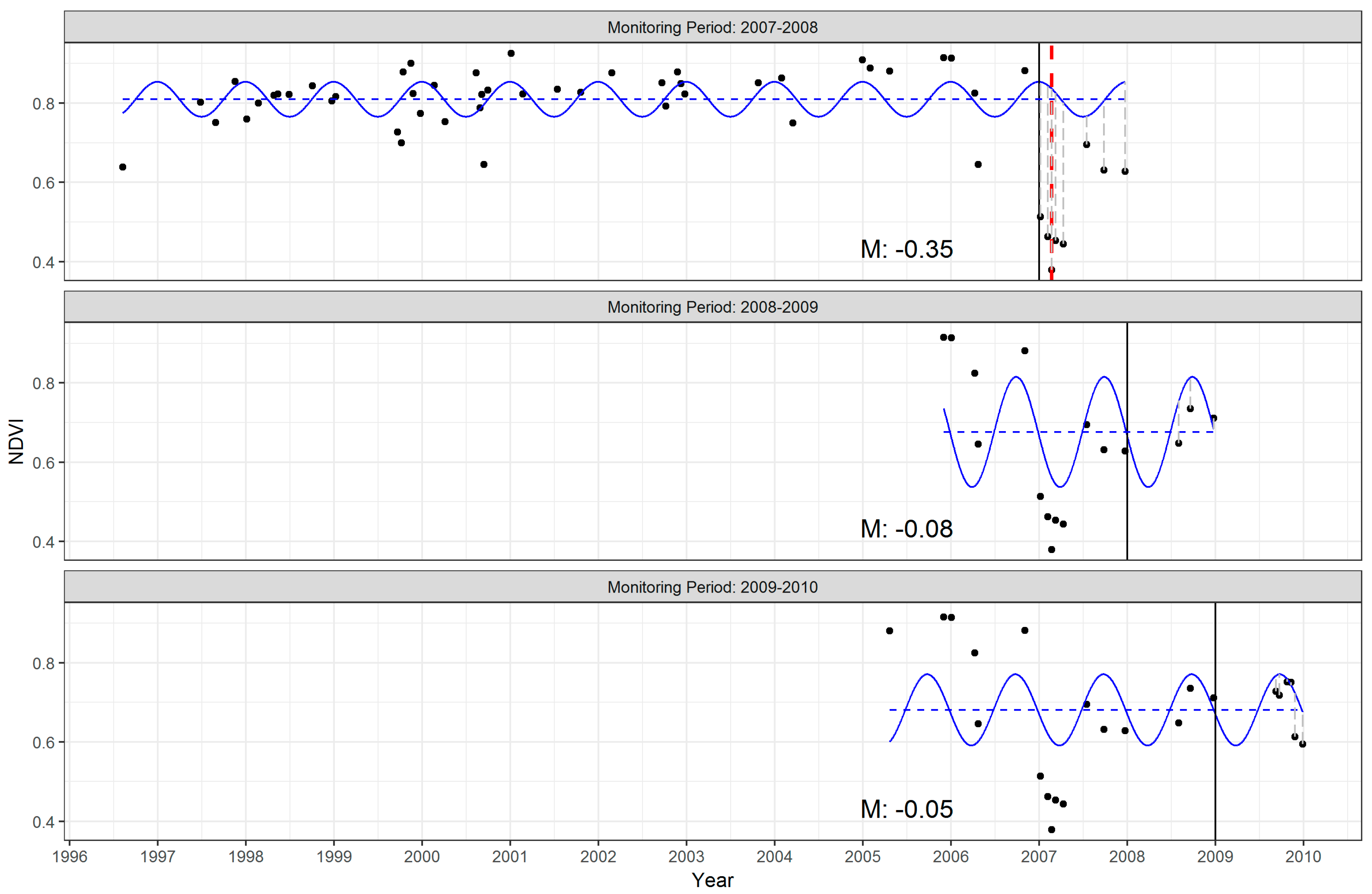
2.5. Landsat-Based Disturbance Detection with BFAST Monitor

Using the Landsat time series, we applied BFAST Monitor to map forest disturbance in Picachos given its proven robustness at detecting disturbance in other tropical forests [58]. BFAST Monitor differs from the conventional BFAST algorithm that we used with the MAIAC time series in three important ways. First, we only fit a first-order harmonic curve to the Landsat time series using BFAST Monitor, whereas we used a third-order harmonic for the MAIAC time series. This decision lies in the irregular distribution of Landsat observations that can result in model over-fitting [14]. Second, we omitted the trend component when modeling the Landsat time series but used a seasonal-and-trend model with MAIAC. The inclusion of a trend component in modeling the Landsat time series would have generated erroneously modeled NDVI values in the monitoring period. Third, BFAST extracted major breaks by considering the MAIAC time series as a whole, while BFAST Monitor evaluated potential breaks across the Landsat time series in a succession of one year-long periods.
We used 32 Landsat images collected between 1996 and 2000 to develop a historical baseline of forest cover trends. Because using all images may have affected the BFAST Monitor model fit [32], we measured the reversed-ordered-cumulative (ROC) sum of residuals to generate a cumulative prediction error that helps identify whether a seasonal model no longer offers an accurate fit [59] (Figure 3). With the historical model in place, we applied BFAST Monitor sequentially from 2001 to 2015, following the approach by DeVries at al. [14].
The detection of breakpoints using BFAST Monitor is associated with near-zero or positive magnitudes which could not be related to forest disturbance [14]. The breakpoint magnitude is calculated as the median of observation-model residuals within each monitoring period [32]. In identifying the magnitude threshold to distinguish disturbance from non-disturbance and minimize spurious breakpoints, we selected a stratified random sample of 420 breakpoints based on three magnitude quantiles from the study area where very high resolution images from Google Earth were available for 2004 and 2009. We classified sample points as being disturbed or non-disturbed based on visual interpretation of true color imagery as well as NDVI time series. We then calculated a magnitude threshold of −0.041 using Binomial Logistic Regression where the likelihood of actual disturbance approached 50% (Figure S2) [60]. We considered any potential breakpoint with a magnitude less than −0.041 to be disturbed [61].

2.6. Validation and Agreement Assessment

BFAST Monitor validation approaches in tropical regions typically involve a single image, which makes it difficult to capture annual dynamics or disturbed areas [14,25]. To overcome this limitation, we used sub-annual Landsat L1T-derived NDVI imagery, Google Earth-hosted annual Landsat true color images and very high resolution images (2003–2004, 2007 and 2009), and RapidEye images (2014–2015). We visually inspected disturbance sites and identified obviously erroneous disturbances, such as pixels influenced by river dynamics.
With erroneous disturbance sites removed, we sampled 684 validation sites following Cochran’s recommendations [62]. After removing 24 sample sites due to lack of images, we distributed the remaining 660 sites into disturbed and non-disturbed sample sets following Olofsson et al. [63]; this yielded 269 disturbed and 391 initial non-disturbed sites. Given that the amount of disturbed forest in Picachos is expected to be relatively small compared to stable forest or otherwise non-disturbed sites, we sought to decrease the potential overrepresentation of non-disturbed sites in the validation sample by stratifying a non-disturbed validation sample with respect to a 2 km buffer from unpaved roads (2014–2015) derived from high-resolution images [34] with the assumption that disturbed sites are likely closer to roads [64,65,66]. Our final validation sample includes 151 non-disturbed sites within the road buffer, and 240 non-disturbed sites outside the buffer.
For each disturbed site, we evaluated the temporal agreement of BFAST Monitor-derived disturbances against our reference datasets (Google Earth, Rapideye and NDVI sub-annual scenes) using 20 sampled pixels per year into TimeSync [31] (as adapted in R by DeVries et al. [14]). A pixel-count confusion matrix was derived from every strata, and we removed the bias effect of unequal omission and commission errors by constructing an area-adjusted error matrix [63,67]. We calculated the stratified estimator for a given class as:
A ^ j = A ^ t o t a l × p ^ .   j
where A ^ j is the adjusted area, A ^ t o t a l is the total mapped area for a given class, and p ^ .   j is the column sum of the cell area proportion in the error matrix. We further validated MAIAC trends using Landsat-based disturbance events by comparing the timeline of MAIAC-based breakpoints with annual Landsat-based disturbances.

3. Results

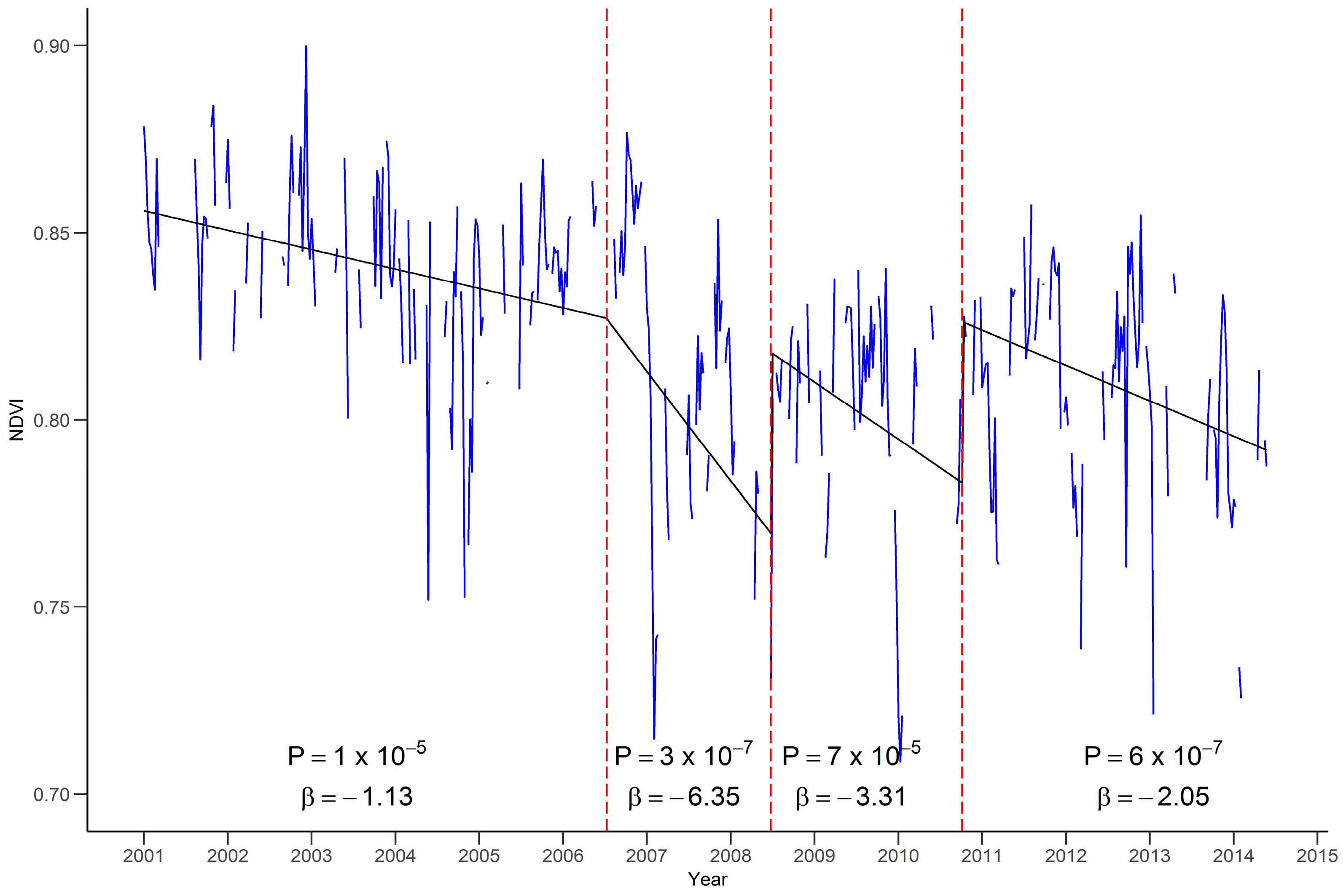
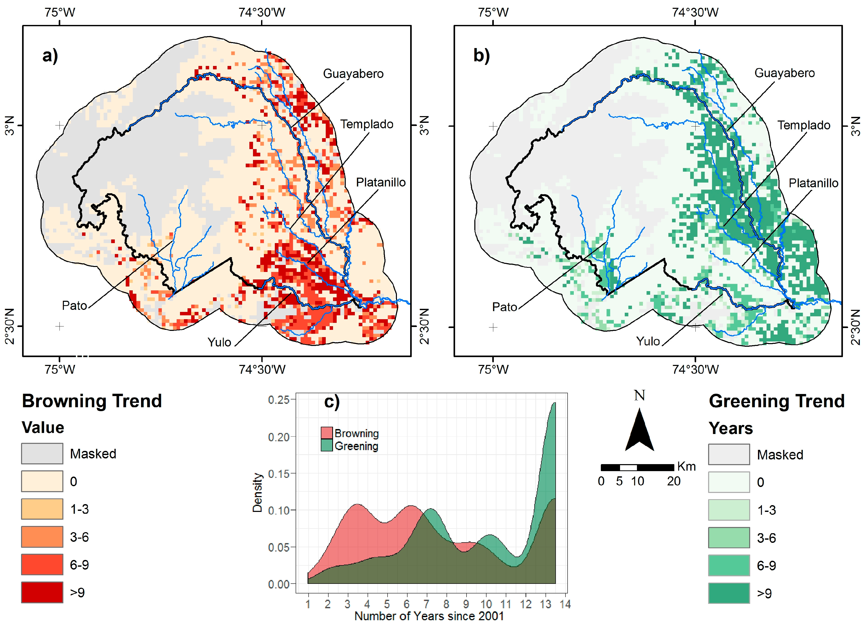
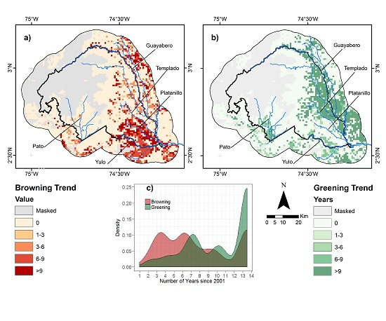
3.1. MAIAC-Derived Browning and Greening Patterns

The most prominent browning region is in the southeastern corner of Picachos with small and scattered browning regions beyond the park’s northeastern perimeter near small settlements (Figure 4a). The watershed most affected by persistent browning is the Platanillo River watershed while the Templado River watershed is only affected at its southern extent where it merges with adjacent watersheds. The Yulo River watershed presented both browning and greening over our study period with more greening evident within Picachos. Greening clusters (Figure 4b) were found on a steeply sloped region in the park’s central-south region and surrounded by a river, the Rio Pato, and also in the central-eastern foothills along the large rivers, the Rio Guayabero and Rio Leiva. Within the park, 12,500 ha showed 13 years of consecutive browning, whereas the total area of persistent greening amounted to 27,700 ha.
Each pixel may exhibit greening or browning at different periods over the time series (Figure 4). To calculate the percentage of Picachos that experienced browning or greening, we divide the total amount of browning and greening pixels by Picachos’ extent as well as the 10 km-wide region surrounding the park. In total, 14% and 20% of the park displayed browning and greening, respectively, while 32% of Picachos was masked due to absence of MAIAC observations due to cloud cover. Within the 10 km-wide region surrounding Picachos, 5% and 2.5% of the surrounding forest exhibited browning and greening, respectively. Therefore, we recorded a total positive (greening) net trend of 6% within Picachos, but a negative (browning) trend of 2.5% surrounding the park.
The lengths of browning periods were generally shorter than greening periods: browning periods frequently lasted 3 or 6 years, while greening tended to last 7 or more than 10.5 years (Figure 4c). Both greening and browning trends occurred at a low elevation between 300–600 m and during 2004–2007. Fifty percent of pixels in the park had MAIAC trends with zero breakpoints over the 2001–2014 study period, 12% of the park saw a single breakpoint, while 4.5% of the park saw two or more breakpoints during the study period, most of which occurred in the southeastern corner of the park.

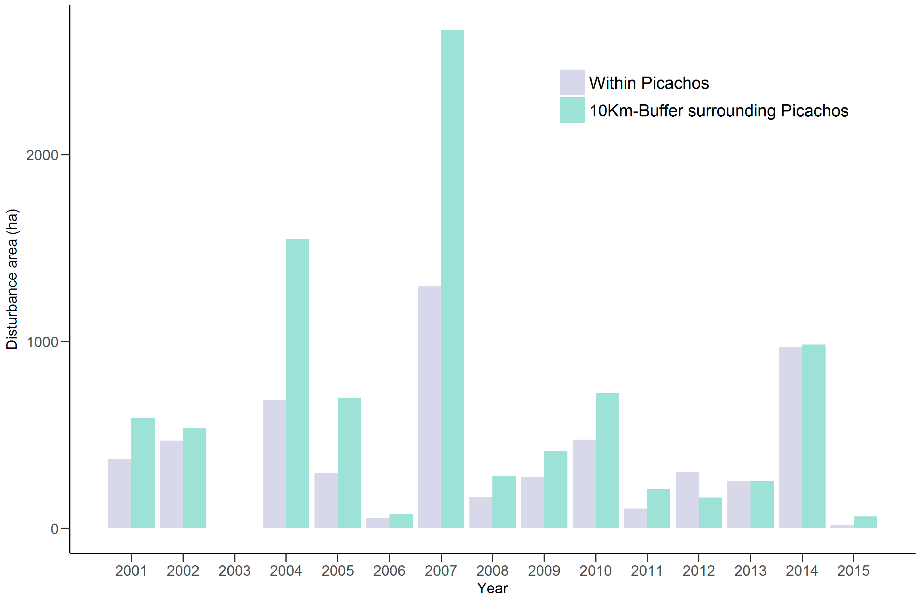
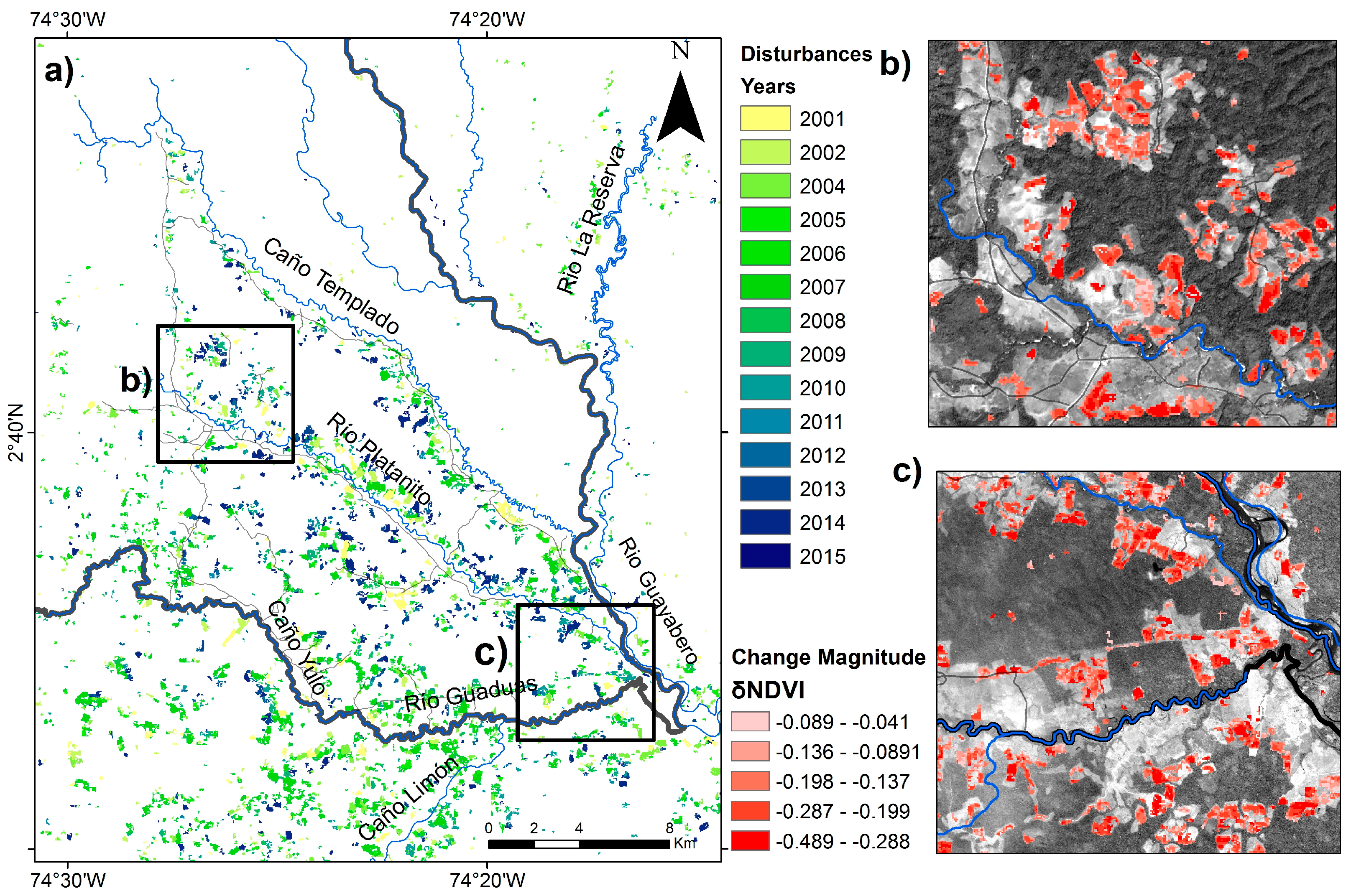
3.2. Landsat-Based Disturbance Distribution

Using BFAST Monitor with Landsat data, we measured a total of 6353 ha of disturbed area within Picachos from 2001–2015 and 6289 ha disturbed area between 1998 and 2001, yielding a total disturbed area of 12,642 ha (±1440 margin of error, 95% confidence interval) or 4.3% of Picachos’ total area. This disturbed area estimate is 20% less than the previous estimate of 15,276 ha based on the CLC methodology [34]. This difference can be explained by the poor validation of the CLC dataset in this region, differences in cloud-masking approaches, and, further, that inter-annual change maps based on CLC datasets suggest forest cover change in many regions despite the presence of visually interpreted stable forest.
As with the spatial distribution of MAIAC browning trends, Landsat disturbances were concentrated in the southeast with scattered disturbance recorded in the northeast just outside Picachos (Figure 5). The mean size of Landsat-derived disturbed patches is 1.9 ha (range 1.1–2.9 ha) across all years, while the maximum annual mean patch size is 19.8 ha (range 5.1–49.3 ha). The size of disturbed patches within Picachos is considerably larger than the 0.6 ha patch size in other tropical forest regions [14], but is smaller than the 8–10 ha patch size in other mountainous regions [10]. During 2001–2015, the total disturbance area within the 10 km-wide region surrounding Picachos was 9218 ha, which is 1.6 times greater than the total amount of disturbance within the park. The years 2004 and 2007 witnessed the most disturbance in the region surrounding Picachos, whereas 2007 and 2014 exhibited the most change within the park (Figure 6).

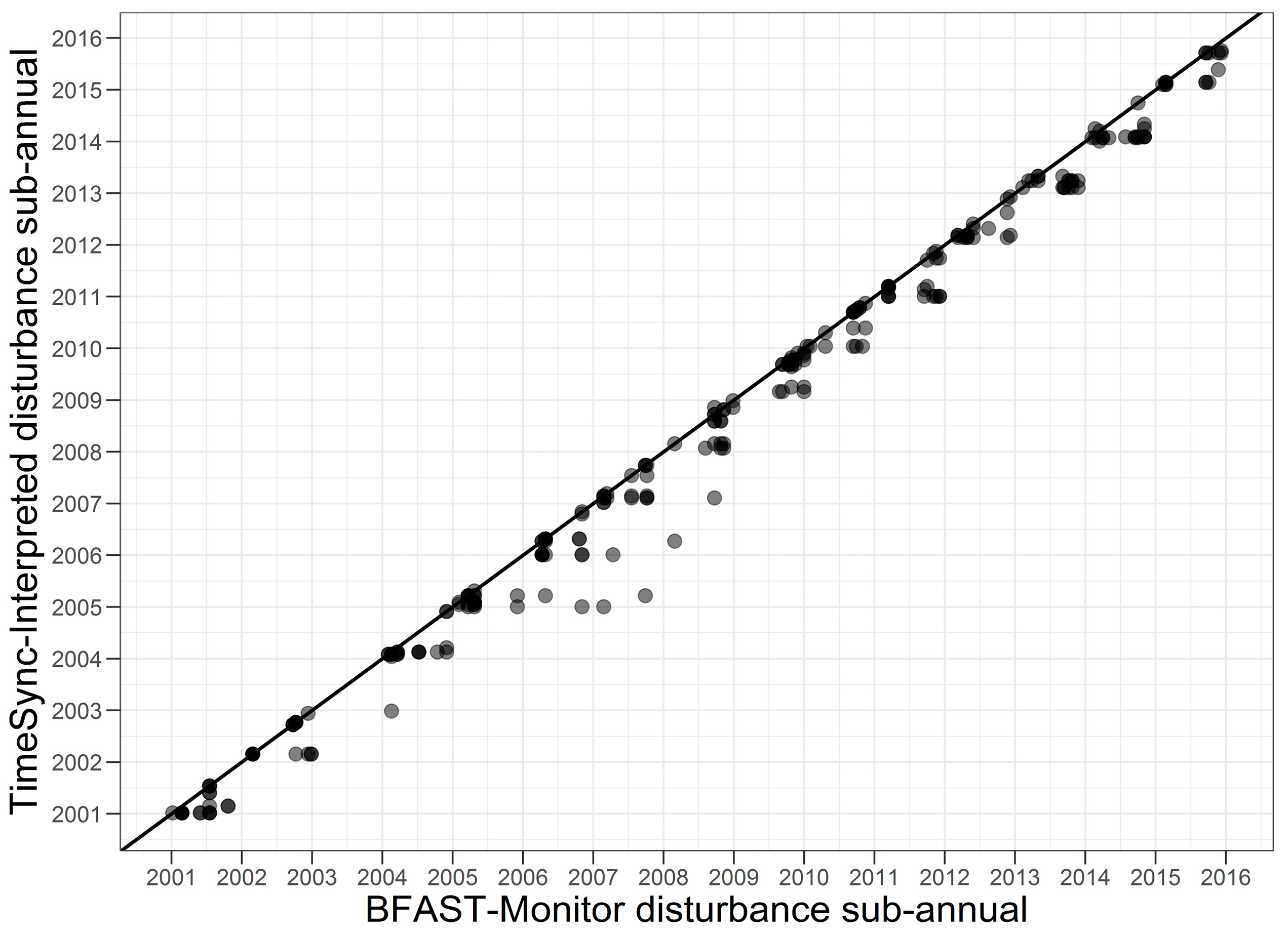
3.3. Validation of Landsat-Derived Disturbances

Using 660 validation points, we recorded a high total accuracy (TA) of 0.99 ± 0.007 for disturbed class sites, with user’s (UA) and producer’s accuracies (PA) of 0.95 ± 0.024 and 0.83 ± 0.18, respectively. The non-disturbed classes presented a combined UA of 0.98 ± 0.026 and PA of 0.99 ± 0.002 (Table 1). Accuracies were similar to previous studies in South America [60], but higher in comparison with other tropical regions [29]. We also assessed the agreement between Landsat-based BFAST Monitor disturbance dates and TimeSync-interpreted disturbance dates based on sub-annual Landsat true color, sub-annual Landsat L1T-derived NDVI scenes and supporting very high resolution imagery. Most disturbance dates showed an agreement of 75% within ±6 months, while the bulk of other disturbances (22%) showed a residual of 6−12 months; and 3% of remaining errors showed disagreement greater than 12 months (Figure 7).

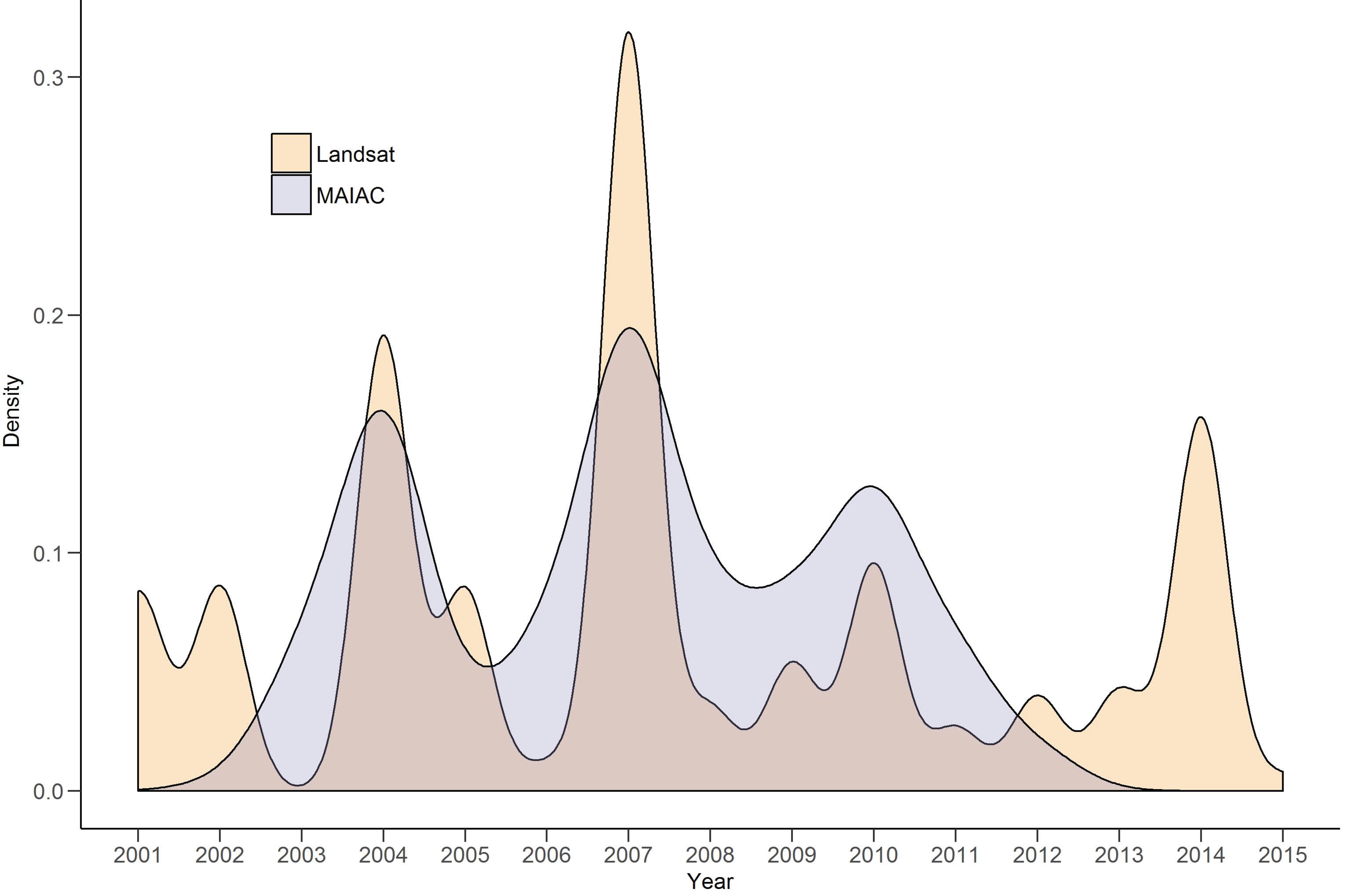
3.4. Validation of MAIAC Breakpoints

The most frequent year of MAIAC breakpoints was 2007, followed by 2004 and 2010, which coincide with the most frequent years of Landsat disturbance between 2002 and 2013 (Figure 8). Although MAIAC time series data spanned from January 2001 to June 2014, no significant breaks were detected during 2001–2002 and 2013–2014. This is due to the h-defined minimum segment size of 2.03 years that restricted our ability to detect breakpoints at the beginning and end of the time series but supported accurate model fitting within each segment [32,46,68]. The pattern of Landsat disturbances is more temporally-resolved because of the year-by-year sequential monitoring used by BFAST Monitor. Nonetheless, the agreement in timing and location of major changes observed in MAIAC and Landsat time series confirms the potential of coarse spatial resolution time series to accurately capture the broad-scale multi-year trajectory of forest disturbance.

4. Discussion

In this study, we demonstrated the ability of BFAST-based methods to accurately detect short- and long-term disturbances over a mountainous forest reggion. This is also the first study to combine all available Landsat 5, 7, and 8 images using BFAST Monitor and account for radiometric and spectral differences between TM/ETM+ and OLI sensors; while DeVries et al. [30] used the same sensors within BFAST but did not consider the potential bias in cross-sensor NDVI measurements [54,55]. Accounting for this bias is critical since the bias magnitude may approach or exceed the threshold selected to identify disturbance [14,28,60].

4.1. Possible Drivers of Vegetation Trends and Disturbances

Picachos and its surrounding region have been affected by social conflict and population displacement since as early as 1991 [34]. From 1998–2002, FARC-EP (Fuerzas Armadas de Colombia-Ejercito del Pueblo) was legally sited in San Vicente del Caguán, neighboring Picachos to the south, as part of a negotiation process conducted by the former Colombian government. However, this agreement collapsed and the increased violence associated with the conflict between FARC and the Colombian government has been widely recognized as generating both internal displacement and economic migration into Picachos, particularly in the accessible southeastern region [34,35,69]. The increased in-migration accelerated the expansion of unpaved roads and infrastructure (small settlements) as well as selective logging and clearing for crops and cattle pasture, all of which has contributed to deforestation in the park [34,35]. Such changes in land cover and land use have been documented in a peasant reserve close to Picachos’ southern boundary, Losada-Guayabero, which includes more than 2000 families with agricultural and pastoral livelihoods [34,35]. The changes in dominant land use coincides with the concentration of browning trends and small-scale disturbances in the southeastern foothills of Picachos as detected by both MAIAC and Landsat and corroborated in previous studies [4,12,34,70] (Figure 9). Conversely, the concentration of MAIAC-based greening trends and absence of Landsat-based disturbance near large rivers in eastern Picachos, such as Rio Guayabero, suggests that these rivers act as barriers to forest resource extraction.
The abundance of disturbance events between 2004 and 2010 is likely a consequence of increased beef consumption in Colombia in the mid-2000s [71] and the growth of the livestock industry from 20 to 23 million head from 2001–2010 before stabilizing over 2011–2014 [72]. Furthermore, Picachos is sited in the provinces of Meta and Caquetá, provinces that saw a high growth of livestock production to supply the domestic market [73], which has encroached upon Picachos and its surroundings.
The increase in disturbance surrounding Picachos had its roots in agrarian policies that have contributed to the intensification of agricultural land uses over lowlands and foothills within the region [69]. These policies promoted an initial process of occupation and accumulation of land followed by the establishment of production models based on agricultural and livestock-based land use systems [35]. The changes brought by these formal land use policies were subsequently exacerbated by other regional processes such as: (1) expansion of illegal crops; (2) forced displacement due to armed conflict; and (3) lack of records of land titles and hence land tenure, which have often resulted in an informal and unrecognized appropriation of land [34]. While a broader discussion of socio-economic drivers is warranted, such an examination is made difficult by lack of field and demographic data, as well as accessibility to the study site.

4.2. Effectiveness of BFAST Disturbance Detection Methods

Both BFAST implementations supported detection of vegetation change with high spatial and temporal accuracies. Though the MAIAC time series has a coarse spatial resolution, its high temporal resolution, improved cloud detection technique, and exceptional mitigation of sun-sensor geometry supported a refined detection of breakpoints that was broadly confirmed using a year-to-year Landsat-based disturbance monitoring approach. The most abrupt changes in the Landsat time series were recorded in 2004, 2007, 2010 and 2014. Our detection of such abundant changes despite the low average of 8 Landsat images per year from 2001–2015 suggests that having a relatively low number of images during the monitoring period had little effect on our ability to detect disturbances (See Table S1).
The Landsat-based disturbance class presented a high spatial and temporal agreement with the majority of errors (22%) resulting from a 6–12 month premature assignation of disturbance. Omission errors (17%) could have been improved by increasing the density of the time series [58], whereas commission errors (5%) could have benefitted by stratifying validation site samples according to likelihood of vegetation change, such as locations along the park border, along unpaved roads, or near rivers.
The reference datasets employed showed agreement in disturbance timing at over 75% of sampled sites when compared to our TimeSync-based interpretation. NDVI also performs well despite its well-known saturation issues over areas with high biomass values. One reason NDVI was useful is likely because the rapid alteration of Picachos was more readily detected than gradual or low-intensity change disturbances over time. Had this not been the case, the NDVI performance may have suffered, prompting us to pursue another vegetation index [58]. Other approaches such as Spatial Temporal Adaptive Algorithm for mapping Reflectance Change (STAARCH) [74] or the Noise Insensitive Trajectory Algorithm (NITA) [16] would have been useful in estimating trends over these mountainous and persistently cloudy places.

4.3. Other Limitations

This study provides new insights into the contribution of small-scale disturbances and long-term trends over a 15-year period in one of the most inaccessible national parks in the Andes. While we have recorded short- and long-term changes in Picachos using multi-sensor time series data with high spatial and temporal agreement, there are three main areas for improvement in future studies. Disturbance detection was not possible over 32% of Picachos, primarily at the highest elevations where cloud cover was near-constant. While we expect there to be minimal human-induced disturbance at elevations over 2000 m above sea level [34,35], the lack of cloud-free observations means we cannot examine potential climate change-related vegetation degradation. As with other studies [14,58], we do not specifically identify vegetation recovery and assumed that a BFAST Monitor-detected breakpoint with a magnitude less than our threshold (−0.041) symbolized a permanent change. Although this assumption is reasonable for land cover conversion caused by land use changes such as livestock management and road expansion, it may not be appropriate for detecting natural disturbances. Furthermore, we do not make any differentiation between deforestation and degradation. Though NDVI is sensitive to significant change in vegetation conditions, NDVI alone may not support detection of forest thinning or degradation [30].
Greening and browning indicators from MAIAC are only represented in terms of individual significant slope (β) segments. Although the magnitude of change may have value for classifying the severity of disturbance (i.e., gradual or abrupt), the majority of magnitude values were small: browning magnitudes ranged from −0.318 to −0.00072 (mean = −0.055), whereas greening ranged from 0.0005 to 0.239 (mean = 0.05). These values must be interpreted with caution due to pixel size and NDVI saturation issues over dense forest.
Although we reached high disturbance detection accuracies, omission errors suggest that data availability is still a problem. As with many other disturbance analyses in tropical regions, our lack of Landsat coverage during the 1990s affects our ability to continuously monitor long-term changes [14,75]. In our case, zero Landsat images are available between 1992 and 1995. Given this, it would be valuable to include observational data such as synthetic aperture radar [76], Sentinel 1–2 [77], or very high resolution commercial imagery from Planet Labs, for example [78]. A related limitation stems from the masking procedure combining Hansen et al. [56] and European Space Agency Corine land cover products, neither of which are well validated for this study area.
Finally, we do not perform a quantitative attribution of change events to specific agents of disturbance. Of special interest, the impact of armed conflict over land use changes and internally displaced people along with illegal land appropriation has not been sufficiently explored, nor have the effects of forced displacement on the potential for forest recovery. Investigation of such topics would make for a promising future study.

5. Conclusions

In this study, we recorded short-term disturbances and long-term trends of forest disturbance in Picachos National Park within the Colombian Andes from 2001–2015. We implemented and validated two approaches based on BFAST, neither of which had been tested over persistently cloudy regions. Our BFAST implementations using MAIAC and Landsat identified greening and browning periods based on significant trend segments as well as smaller disturbances with relatively high spatial and temporal accuracies. We identified an abundance of greening within Picachos, albeit with a hotspot of vegetation decline in the park’s southeastern foothills region that likely results from population incursion and land use conversion. This study was limited by a lack of MAIAC and Landsat observations at higher elevations, which affects both our long-term evaluation of forest trends as well as evaluation of short-term ecological processes. Although MAIAC offers a coarse spatial resolution, our results show that MAIAC-based time series can effectively detect hotspots of vegetation decline where Landsat data are not available.

Supplementary Materials

The following are available online at www.mdpi.com/2072-4292/9/2/179/s1, Figure S1: Percentage of cloud-free Landsat observation in the period 1996–2015, Figure S2: Selection of magnitude threshold (P(disturbances) = 0.5) using Binomial Logistic Regression. The grey area is 95% confident interval. Training sites (blue points) were selected based on visual interpretation where 0 = non-disturbed and 1 = disturbed, Table S1: Total number of Landsat images used for disturbance detection.

Acknowledgments

Universidad del Tolima (Colombia) and Oregon State University supports P.J.M.S. Cormacarena and Parques Nacionales de Colombia provided Corine Land Cover dataset and Rapideye Images. We also thank NASA for providing MAIAC time series for South America. Finally, the United States Geological Survey (USGS) maintains and makes available the Landsat archive. We are thankful to the three anonymous reviewers whose comments greatly improved this manuscript. Thomas Hilker, whose knowledge, humility and generosity made this work possible. For him, all our gratitude, admiration and affection.

Author Contributions

Paulo J. Murillo-Sandoval and Thomas Hilker conceived and designed this research. Paulo J. Murillo-Sandoval and Jamon Van Den Hoek performed data processing and interpretation. All authors contributed to the paper’s writing.

Conflicts of Interest

The authors declare no conflict of interest.

References

  1. Wiens, J.; Sutter, R.; Anderson, M.; Blanchard, J.; Barnett, A.; Aguilar-Amuchastegui, N.; Avery, C.; Laine, S. Selecting and conserving lands for biodiversity: The role of remote sensing. Remote Sens. Environ. 2009, 113, 1370–1381. [Google Scholar] [CrossRef]
  2. Myers, N.; Fonseca, G.A.B.; Mittermeier, R.A.; Fonseca, G.A.B.; Kent, J. Biodiversity hotspots for conservation priorities. Nature 2000, 403, 853–858. [Google Scholar] [CrossRef] [PubMed]
  3. Jetz, W.; Wilcove, D.S.; Dobson, A.P. Projected impacts of climate and land-use change on the global diversity of birds. PLoS Biol. 2007, 5, 1211–1219. [Google Scholar] [CrossRef] [PubMed]
  4. Armenteras, D.; Rodríguez, N.; Retana, J.; Morales, M. Understanding deforestation in montane and lowland forests of the Colombian Andes. Reg. Environ. Chang. 2011, 11, 693–705. [Google Scholar] [CrossRef]
  5. Sánchez-Cuervo, A.M.; Aide, T.M. Consequences of the Armed conflict, forced human displacement, and land abandonment on forest cover change in Colombia: A multi-scaled analysis. Ecosystems 2013, 16, 1052–1070. [Google Scholar] [CrossRef]
  6. Portillo-Quintero, C.A.; Sanchez, A.M.; Valbuena, C.A.; Gonzalez, Y.Y.; Larreal, J.T. Forest cover and deforestation patterns in the Northern Andes (Lake Maracaibo Basin): A synoptic assessment using MODIS and Landsat imagery. Appl. Geogr. 2012, 35, 152–163. [Google Scholar] [CrossRef]
  7. Josse, C.; Cuesta, F.; Gonzalo Navarro, V.; Becerra, M.T.; Cabrera, E.; Chacón-Moreno, E.; Ferreira, W.; Peralvo, M.; Saito, J.; Tovar, A.; Naranjo, L. Physical geography and ecosystems in the tropical Andes. In Climate Change and Biodiversity in the Tropical Andes, Inter-American Institute for Global Change Research (IAI) and Scientific Committee on Problems of the Environment (SCOPE); Herzog, S., Martinez, R., Jorgensen, P.M., Tiessen, H., Eds.; São José dos Campos y París: Paris, Frence, 2011; p. 348. [Google Scholar]
  8. Simula, M.; Mansur, E. A global challenge needing local response. Unasylva 2011, 62, 3–7. [Google Scholar]
  9. Willis, K.S. Remote sensing change detection for ecological monitoring in United States protected areas. Biol. Conserv. 2015, 182, 233–242. [Google Scholar] [CrossRef]
  10. Fernández, G.; Obermeier, W.; Gerique, A.; Sandoval, M.; Lehnert, L.; Thies, B.; Bendix, J. Land cover change in the Andes of Southern Ecuador—Patterns and drivers. Remote Sens. 2015, 7, 2509–2542. [Google Scholar] [CrossRef]
  11. Rodríguez, N.; Armenteras, D.; Retana, J. Effectiveness of protected areas in the Colombian Andes: Deforestation, fire and land-use changes. Reg. Environ. Chang. 2013, 13, 423–435. [Google Scholar] [CrossRef]
  12. Armenteras, D.; Gast, F.; Villareal, H. Andean forest fragmentation and the representativeness of protected natural areas in the eastern Andes, Colombia. Biol. Conserv. 2003, 113, 245–256. [Google Scholar] [CrossRef]
  13. Tovar, C.; Seijmonsbergen, A.C.; Duivenvoorden, J.F. Monitoring land use and land cover change in mountain regions: An example in the Jalca grasslands of the Peruvian Andes. Landsc. Urban Plan. 2013, 112, 40–49. [Google Scholar] [CrossRef]
  14. DeVries, B.; Verbesselt, J.; Kooistra, L.; Herold, M. Robust monitoring of small-scale forest disturbances in a tropical montane forest using Landsat time series. Remote Sens. Environ. 2015, 161, 107–121. [Google Scholar] [CrossRef]
  15. Van den Hoek, J.; Ozdogan, M.; Burnicki, A.; Zhu, A.X. Evaluating forest policy implementation effectiveness with a cross-scale remote sensing analysis in a priority conservation area of Southwest China. Appl. Geogr. 2014, 47, 177–189. [Google Scholar] [CrossRef]
  16. Alonzo, M.; van den Hoek, J.; Ahmed, N. Capturing coupled riparian and coastal disturbance from industrial mining using cloud-resilient satellite time series analysis. Sci. Rep. 2016, 6, 35129. [Google Scholar] [CrossRef] [PubMed]
  17. Anaya, J.A.; Colditz, R.R.; Valencia, G.M. Land cover mapping of a tropical region by integrating multi-year data into an annual time series. Remote Sens. 2015, 7, 16274–16292. [Google Scholar] [CrossRef] [Green Version]
  18. Instituto de Hidrología Meteorología y Estudios Ambientales de Colombia (IDEAM). Leyenda nacional de coberturas de la tierra. Metodologia CORINE Land Cover Adaptada para Colombia Escala 1:100000; IDEAM: Bogota, Colombia, 2010. [Google Scholar]
  19. Hilker, T.; Lyapustin, A.I.; Tucker, C.J.; Sellers, P.J.; Hall, F.G.; Wang, Y. Remote sensing of tropical ecosystems: Atmospheric correction and cloud masking matter. Remote Sens. Environ. 2012, 127, 370–384. [Google Scholar] [CrossRef]
  20. Hilker, T.; Lyapustin, A.I.; Hall, F.G.; Myneni, R.; Knyazikhin, Y.; Wang, Y.; Tucker, C.J.; Sellers, P.J. On the measurability of change in Amazon vegetation from MODIS. Remote Sens. Environ. 2015, 166, 233–242. [Google Scholar] [CrossRef]
  21. Hilker, T.; Lyapustin, A.I.; Tucker, C.J.; Hall, F.G.; Mynen, R.B.; Wang, Y.; Bi, J.; Sellers, P.J. Vegetation dynamics and rainfall sensitivity of the Amazon. Proc. Natl. Acad. Sci. USA 2014, 111, 16041–16046. [Google Scholar] [CrossRef] [PubMed]
  22. Bi, J.; Myneni, R.; Lyapustin, A.; Wang, Y.; Park, T.; Chi, C.; Yan, K.; Knyazikhin, Y. Amazon forests’ response to droughts: A perspective from the MAIAC product. Remote Sens. 2016, 8, 1–12. [Google Scholar] [CrossRef]
  23. Achard, F.; Beuchle, R.; Mayaux, P.; Stibig, H.J.; Bodart, C.; Brink, A.; Carboni, S.; Desclée, B.; Donnay, F.; Eva, H.D.; et al. Determination of tropical deforestation rates and related carbon losses from 1990 to 2010. Glob. Chang. Biol. 2014, 20, 2540–2554. [Google Scholar] [CrossRef] [PubMed]
  24. Achard, F.; Stibig, H.-J.; Eva, H.D.; Lindquist, E.J.; Bouvet, A.; Arino, O.; Mayaux, P. Estimating tropical deforestation from Earth observation data. Carbon Manag. 2010, 1, 271–287. [Google Scholar] [CrossRef]
  25. Dutrieux, L.P.; Verbesselt, J.; Kooistra, L.; Herold, M. Monitoring forest cover loss using multiple data streams, a case study of a tropical dry forest in Bolivia. ISPRS J. Photogramm. Remote Sens. 2015, 107, 112–125. [Google Scholar] [CrossRef]
  26. Kennedy, R.E.; Yang, Z.; Cohen, W.B. Detecting trends in forest disturbance and recovery using yearly Landsat time series: 1. LandTrendr—Temporal segmentation algorithms. Remote Sens. Environ. 2010, 114, 2897–2910. [Google Scholar] [CrossRef]
  27. Huang, C.; Goward, S.N.; Masek, J.G.; Thomas, N.; Zhu, Z.; Vogelmann, J.E. An automated approach for reconstructing recent forest disturbance history using dense Landsat time series stacks. Remote Sens. Environ. 2010, 114, 183–198. [Google Scholar] [CrossRef]
  28. Hamunyela, E.; Verbesselt, J.; Herold, M. Using spatial context to improve early detection of deforestation from Landsat time series. Remote Sens. Environ. 2016, 172, 126–138. [Google Scholar] [CrossRef]
  29. Schultz, M.; Clevers, J.G.P.W.; Carter, S.; Verbesselt, J.; Avitabile, V.; Quang, H.V.; Herold, M. Performance of vegetation indices from Landsat time series in deforestation monitoring. Int. J. Appl. Earth Obs. Geoinf. 2016, 52, 318–327. [Google Scholar] [CrossRef]
  30. Devries, B.; Pratihast, A.K.; Verbesselt, J.; Kooistra, L.; Herold, M. Characterizing forest change using community-based monitoring data and landsat time series. PLoS ONE 2016, 11, 1–25. [Google Scholar] [CrossRef] [PubMed]
  31. Cohen, W.B.; Yang, Z.; Kennedy, R. Detecting trends in forest disturbance and recovery using yearly Landsat time series: 2. TimeSync—Tools for calibration and validation. Remote Sens. Environ. 2010, 114, 2911–2924. [Google Scholar] [CrossRef]
  32. Verbesselt, J.; Zeileis, A.; Herold, M. Near real-time disturbance detection using satellite image time series. Remote Sens. Environ. 2012, 123, 98–108. [Google Scholar] [CrossRef]
  33. Dudley, N. Guidelines for Applying Protected Area Management Categories; IUCN: Gland, Switzerland, 2008. [Google Scholar]
  34. Unidad Administrativa Especial del Sistema de Parques Nacionales Naturales, Plan de Manejo Coordillera de los Picachos; UAESPNN–Dirección Territorial Costa Orinoquia: Neiva, Colombia, 2016; under review.
  35. Unidad Administrativa Especial del Sistema de Parques Nacionales Naturales, Convenio de Asociación Tripartita P.E. GDE.1.4.7.1.14.022 Suscrito entre Parques Nacionales Naturales, Cormacarena y Patrimonio Natural Fondo para la Diversidad y Áreas Protegidas; UAESPNN–Dirección Territorial Costa Orinoquia: Bogota, Colombia, 2015.
  36. Huete, A.; Didan, K.; Miura, T.; Rodriguez, E.; Gao, X.; Ferreira, L. Overview of the radiometric and biophysical performance of the MODIS vegetation indices. Remote Sens. Environ. 2002, 83, 195–213. [Google Scholar] [CrossRef]
  37. Vermote, E.; Kotchenova, S. Atmospheric correction for the monitoring of land surfaces. J. Geophys. Res. Atmos. 2008, 113. [Google Scholar] [CrossRef]
  38. Samanta, A.; Ganguly, S.; Hashimoto, H.; Devadiga, S.; Vermote, E.; Knyazikhin, Y.; Nemani, R.R.; Myneni, R.B. Amazon forests did not green-up during the 2005 drought. Geophys. Res. Lett. 2010. [Google Scholar] [CrossRef]
  39. Samanta, A.; Ganguly, S.; Vermote, E.; Nemani, R.R.; Myneni, R.B. Why Is Remote Sensing of Amazon Forest Greenness So Challenging? Earth Interact. 2012, 16, 1–14. [Google Scholar] [CrossRef]
  40. Grogan, K.; Fensholt, R. Exploring Patterns and Effects of Aerosol Quantity Flag Anomalies in MODIS Surface Reflectance Products in the Tropics. Remote Sens. 2013, 5, 3495–3515. [Google Scholar] [CrossRef]
  41. Zelazowski, P.; Sayer, A.M.; Thomas, G.E.; Grainger, R.G. Reconciling satellite-derived atmospheric properties with fine-resolution land imagery: Insights for atmospheric correction. J. Geophys. Res. 2011, 116, 597–616. [Google Scholar] [CrossRef]
  42. Seddon, A.W.R.; Macias-Fauria, M.; Long, P.R.; Benz, D.; Willis, K.J. Sensitivity of global terrestrial ecosystems to climate variability. Nature 2016, 531, 229–232. [Google Scholar] [CrossRef] [PubMed]
  43. Wilson, A.M.; Jetz, W. Remotely Sensed High-Resolution Global Cloud Dynamics for Predicting Ecosystem and Biodiversity Distributions. PLoS Biol. 2016, 14, 1–20. [Google Scholar] [CrossRef] [PubMed]
  44. Verbesselt, J.; Hyndman, R.; Zeileis, A.; Culvenor, D. Phenological change detection while accounting for abrupt and gradual trends in satellite image time series. Remote Sens. Environ. 2010, 114, 2970–2980. [Google Scholar] [CrossRef]
  45. De Jong, R.; Verbesselt, J.; Schaepman, M.E.; de Bruin, S. Trend changes in global greening and browning: Contribution of short-term trends to longer-term change. Glob. Chang. Biol. 2012, 18, 642–655. [Google Scholar] [CrossRef]
  46. Watts, L.M.; Laffan, S.W. Effectiveness of the BFAST algorithm for detecting vegetation response patterns in a semi-arid region. Remote Sens. Environ. 2014, 154, 234–245. [Google Scholar] [CrossRef]
  47. Forkel, M.; Carvalhais, N.; Verbesselt, J.; Mahecha, M.D.; Neigh, C.S.R.; Reichstein, M. Trend Change detection in NDVI time series: Effects of inter-annual variability and methodology. Remote Sens. 2013, 5, 2113–2144. [Google Scholar] [CrossRef]
  48. Masek, J.G.; Vermote, E.F.; Saleous, N.; Wolfe, R.; Hall, F.G.; Huemmrich, F.; Gao, F.; Kutler, J.; Lim, T.K. 2013. LEDAPS Calibration, Reflectance, Atmospheric Correction Preprocessing Code, Version 2. Available online: http://dx.doi.org/10.3334/ORNLDAAC/1146 (accessed on 21 February 2017).
  49. Zhu, Z.; Woodcock, C.E. Object-based cloud and cloud shadow detection in Landsat imagery. Remote Sens. Environ. 2012, 118, 83–94. [Google Scholar] [CrossRef]
  50. Zhu, Z.; Fu, Y.; Woodcock, C.E.; Olofsson, P.; Vogelmann, J.E.; Holden, C.; Wang, M.; Dai, S.; Yu, Y. Including land cover change in analysis of greenness trends using all available Landsat 5, 7, and 8 images: A case study from Guangzhou, China (2000–2014). Remote Sens. Environ. 2016, 185, 243–257. [Google Scholar] [CrossRef]
  51. Holden, C.E.; Woodcock, C.E. An analysis of Landsat 7 and Landsat 8 underflight data and the implications for time series investigations. Remote Sens. Environ. 2016, 185, 16–36. [Google Scholar] [CrossRef]
  52. Morton, D.C.; Nagol, J.; Carabajal, C.C.; Rosette, J.; Palace, M.; Cook, B.D.; Vermote, E.F.; Harding, D.J.; North, P.R.J. Amazon forests maintain consistent canopy structure and greenness during the dry season. Nature 2014, 506, 1–16. [Google Scholar] [CrossRef] [PubMed]
  53. Chander, G.; Markham, B.L.; Helder, D.L. Summary of current radiometric calibration coefficients for Landsat MSS, TM, ETM+, and EO-1 ALI sensors. Remote Sens. Environ. 2009, 113, 893–903. [Google Scholar] [CrossRef]
  54. Vogelmann, J.E.; Gallant, A.L.; Shi, H.; Zhu, Z. Perspectives on monitoring gradual change across the continuity of Landsat sensors using time-series data. Remote Sens. Environ. 2016, 185, 258–270. [Google Scholar] [CrossRef]
  55. Roy, D.P.; Kovalskyy, V.; Zhang, H.K.; Vermote, E.F.; Yan, L.; Kumar, S.S.; Egorov, A. Characterization of Landsat-7 to Landsat-8 reflective wavelength and normalized difference vegetation index continuity. Remote Sens. Environ. 2016, 185, 57–70. [Google Scholar] [CrossRef]
  56. Hansen, M.C.; Potapov, P.V.; Moore, R.; Hancher, M.; Turubanova, S.A.; Tyukavina, A. High-resolution global maps of forest cover change. Science 2013, 342, 850–853. [Google Scholar] [CrossRef] [PubMed]
  57. Arino, O.; Perez, J.R.; Kalogirou, V.; Defourny, P.; Achard, F. Globcover 2009. Available online: epic.awi.de/31046/1/Arino_et_al_GlobCover2009-a.pdf(accessed on 20 February 2017).
  58. Schultz, M.; Verbesselt, J.; Avitabile, V.; Souza, C.; Herold, M. Error Sources in Deforestation Detection Using BFAST Monitor on Landsat Time Series across Three Tropical Sites. IEEE J. Sel. Top. Appl. Earth Obs. Remote Sens. 2015, 9, 3667–3679. [Google Scholar] [CrossRef]
  59. Pesaran, M.H.; Timmermann, A. Market timing and return prediction under model instability. J. Empir. Financ. 2002, 9, 495–510. [Google Scholar] [CrossRef]
  60. Devries, B.; Verbesselt, J. Tracking disturbance-regrowth dynamics in tropical forests using structural change detection and Landsat time series. Remote Sens. Environ. 2015, 169, 320–334. [Google Scholar] [CrossRef]
  61. Milton, E.J.; Fox, N.P.; Schaepman, M.E. Progress in field spectroscopy. Remote Sens. Environ. 2006, 113, S92–S109. [Google Scholar] [CrossRef]
  62. Cochran, W.G. Sampling Techniques; John Wiley and Sons: New York, NY, USA, 1977; p. 428. [Google Scholar]
  63. Olofsson, P.; Foody, G.M.; Herold, M.; Stehman, S.V.; Woodcock, C.E.; Wulder, M.A. Good practices for estimating area and assessing accuracy of land change. Remote Sens. Environ. 2014, 148, 42–57. [Google Scholar] [CrossRef]
  64. Overton, W.S.; Stehman, S.V. The Horvitz-Thompson Theorem as a Unifying Perspective. Am. Stat. 1995, 49, 261–268. [Google Scholar]
  65. Barber, C.P.; Cochrane, M.A.; Souza, C.M.; Laurance, W.F. Roads, deforestation, and the mitigating effect of protected areas in the Amazon. Biol. Conserv. 2014, 177, 203–209. [Google Scholar] [CrossRef]
  66. Bax, V.; Francesconi, W.; Quintero, M. Spatial modeling of deforestation processes in the Central Peruvian Amazon. J. Nat. Conserv. 2016, 29, 79–88. [Google Scholar] [CrossRef]
  67. Olofsson, P.; Foody, G.M.; Stehman, S.V.; Woodcock, C.E. Making better use of accuracy data in land change studies: Estimating accuracy and area and quantifying uncertainty using stratified estimation. Remote Sens. Environ. 2013, 129, 122–131. [Google Scholar] [CrossRef]
  68. De Jong, R.; Verbesselt, J.; Zeileis, A.; Schaepman, M.E. Shifts in global vegetation activity trends. Remote Sens. 2013, 5, 1117–1133. [Google Scholar] [CrossRef] [Green Version]
  69. Vásquez, T. Papel del conflicto armado en la construcción y diferenciación territorial de la región de El Caguán Amazonía occidental colombiana. Ágora USB 2013, 14, 147–175. [Google Scholar] [CrossRef]
  70. Etter, A.; McAlpine, C.; Wilson, K.; Phinn, S.; Possingham, H. Regional patterns of agricultural land use and deforestation in Colombia. Agric. Ecosyst. Environ. 2006, 114, 369–386. [Google Scholar] [CrossRef]
  71. Federacion Nacional de Ganaderos de Colombia (FEDEGÁN). Análisis del Inventario Ganadero Colombiano Comportamiento y Variables Explicativas; FEDEGÁN: Bogotá, Colombia, 2013; Volume 1, pp. 1–21. [Google Scholar]
  72. Jimenez, N.J.C.; Miranda, F.C.; Gantiva, O.H.D. El sector de ganadería bovina en Colombia. Aplicación de modelos de series de tiempo al inventario ganadero. Rev. Fac. Cienc. Econ. 2008, 16, 165–177. [Google Scholar]
  73. Santos, S. Inventario bovino de Colombia aumentó en 200 mil cabezas. Contexto Ganad. 2015, 1, 1–5. [Google Scholar]
  74. Hilker, T.; Wulder, M.A.; Coops, N.C.; Seitz, N.; White, J.C.; Gao, F.; Masek, J.G.; Stenhouse, G. Generation of dense time series synthetic Landsat data through data blending with MODIS using a spatial and temporal adaptive reflectance fusion model. Remote Sens. Environ. 2009, 113, 1988–1999. [Google Scholar] [CrossRef]
  75. Broich, M.; Hansen, M.C.; Potapov, P.; Adusei, B.; Lindquist, E.; Stehman, S.V. International journal of applied earth observation and geoinformation time-series analysis of multi-resolution optical imagery for quantifying forest cover loss in Sumatra and Kalimantan, Indonesia. Int. J. Appl. Earth Obs. Geoinf. 2011, 13, 277–291. [Google Scholar] [CrossRef]
  76. Reiche, J. Combining SAR and Optical Satellite Image Time Series for Tropical Forest Monitoring; Wageningen University: Wageningen, The Netherlands, 2015. [Google Scholar]
  77. Petrou, Z.I.; Manakos, I.; Stathaki, T. Remote sensing for biodiversity monitoring: A review of methods for biodiversity indicator extraction and assessment of progress towards international targets. Biodivers. Conserv. 2015, 24, 2333–2363. [Google Scholar] [CrossRef]
  78. Houborg, R.; McCabe, M. High-Resolution NDVI from Planet’s Constellation of Earth Observing Nano-Satellites: A New Data Source for Precision Agriculture. Remote Sens. 2016, 8, 768–771. [Google Scholar] [CrossRef]
Figure 1. The study area of Picachos National Park is located in central Colombia at the northern extent of the Andes mountain range.
Remotesensing 09 00179 g001
Figure 2. Example Breaks for Additive Season and Trend (BFAST) output of a browning pixel. Three major breakpoints (dashed red lines) and four segments (black lines) have been identified over the 13.5-year Multi-Angle Implementation of Atmospheric Correction (MAIAC) time series (blue lines) with missing observations due to cloud effects. The slope coefficients (β) are all significant (α = 0.05) and ρ represents p-values.
Remotesensing 09 00179 g002
Figure 3. Example of pixel-level BFAST Monitor output using a 2007–2010 subset of the Landsat time series. Black solid lines denote the beginning of the monitoring period, black dots are observed NDVI observations, blue lines denote expected values from the fitted seasonal model, and grey dashed lines represent the residuals in each monitoring period. A breakpoint (dashed red line) is identified in early 2007 with a magnitude (M) of −0.35 but is not detected in 2008 or 2009. The historical periods for 2008–2009 and 2009–2010 are shorter than the 2007–2008 period because BFAST Monitor only includes preceding observations until the stable seasonal model breaks down.
Remotesensing 09 00179 g003
Figure 4. Duration of MAIAC-based (a) browning and (b) greening trends based on the number of years with significant trends (α = 0.05); and (c) distribution of browning and greening periods across Picachos and its surrounding area.
Remotesensing 09 00179 g004
Figure 5. Cumulative BFAST monitor-derived disturbance based on the Landsat 2001–2015 time series, aggregated to 1 km pixel size for display.
Remotesensing 09 00179 g005
Figure 6. Temporal distribution of disturbance area within Picachos and the surrounding region. The year 2003 was not evaluated because of a lack of Landsat images.
Remotesensing 09 00179 g006
Figure 7. TimeSync-based comparison of sub-annual BFAST Monitor-output disturbance dates against breakpoint dates identified using reference datasets.
Remotesensing 09 00179 g007
Figure 8. Comparison between breakpoint years detected using MAIAC and Landsat-based disturbance analyses across study area.
Remotesensing 09 00179 g008
Figure 9. (a) Disturbance pattern in southeastern Picachos; (b) Change magnitude (δNDVI) subset over Platanillo sector and presence of unpaved roads (2015 RapidEye Red-Edge band background); (c) Subset for Rio Platanillo, Rio Guayabero, and Rio Guaduas (2014 RapidEye Red-Edge band background).
Remotesensing 09 00179 g009
Table 1. Area-weighted error matrix of Landsat-based BFAST Monitor results using stratified sample sites across classes: (1) Disturbance; (2) Non-disturbance outside the 2 km unpaved roads buffer; and (3) Non-disturbance inside the 2 km unpaved roads buffer.
Reference
123Proportion of Area Mapped (Wi)User’s AccuracyProducer’s AccuracyTotal Accuracy
Map10.0270.00010.00110.0280.95 ± 0.0240.83 ± 0.180.99 ± 0.007
20.0020.17200.1740.98 ± 0.0180.99 ± 0.001
30.00300.7930.7970.99 ± 0.0080.99 ± 0.001
Total0.0330.1720.7941

