
Evapotranspiration Estimates Derived Using Multi-Platform Remote Sensing in a Semiarid Region


Abstract
:
1. Introduction
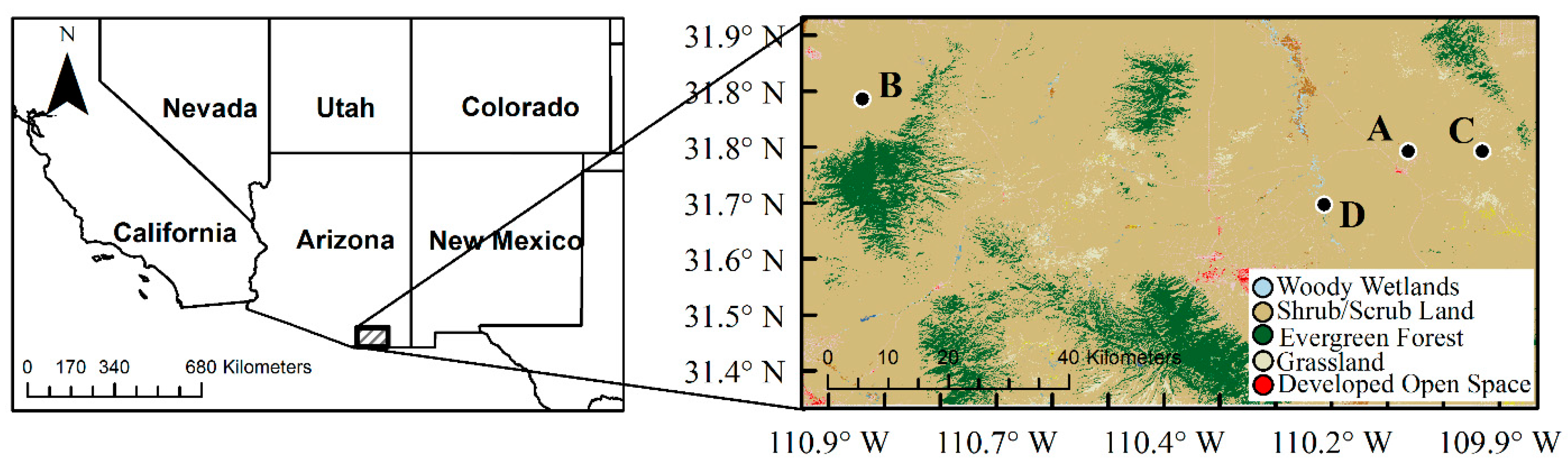
2. Study Area
3. Datasets
3.1. In Situ Measurements
3.2. Satellite Observations (SMOS and MODIS)
3.2.1. SMOS Satellite Observations
3.2.2. Moderate Resolution Imaging Spectroradiometer (MODIS) Observations
3.3. Empirical ET Model
3.4. NLDAS-2 Models
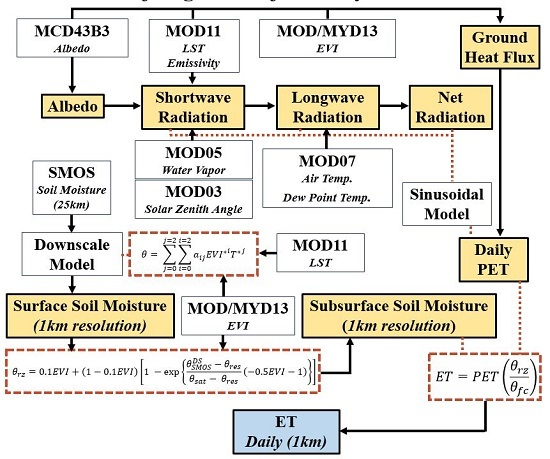
4. Methodology
4.1. PET Estimation
4.2. Soil Moisture Estimation
4.3. Actual Evapotranspiration
5. Results and Discussion
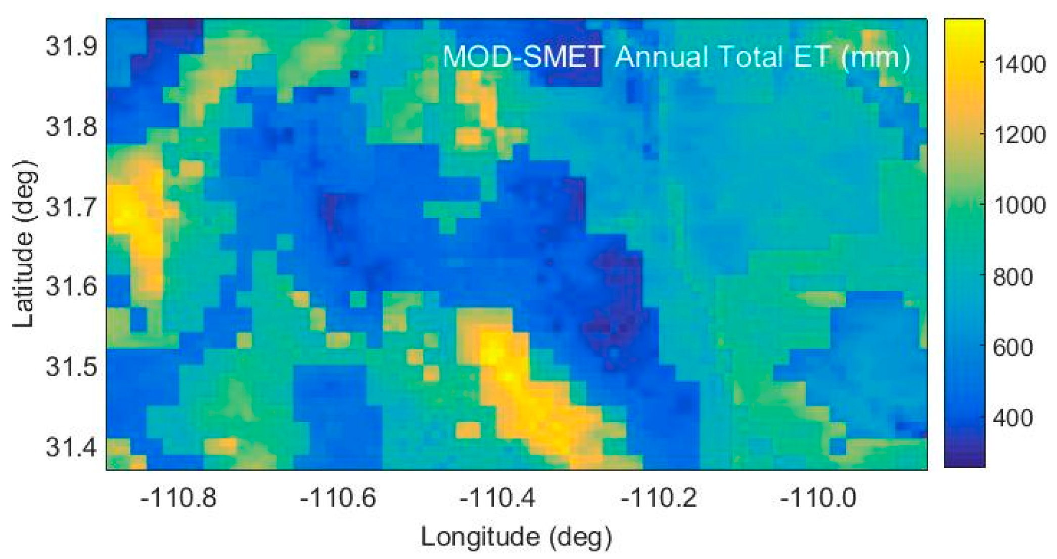
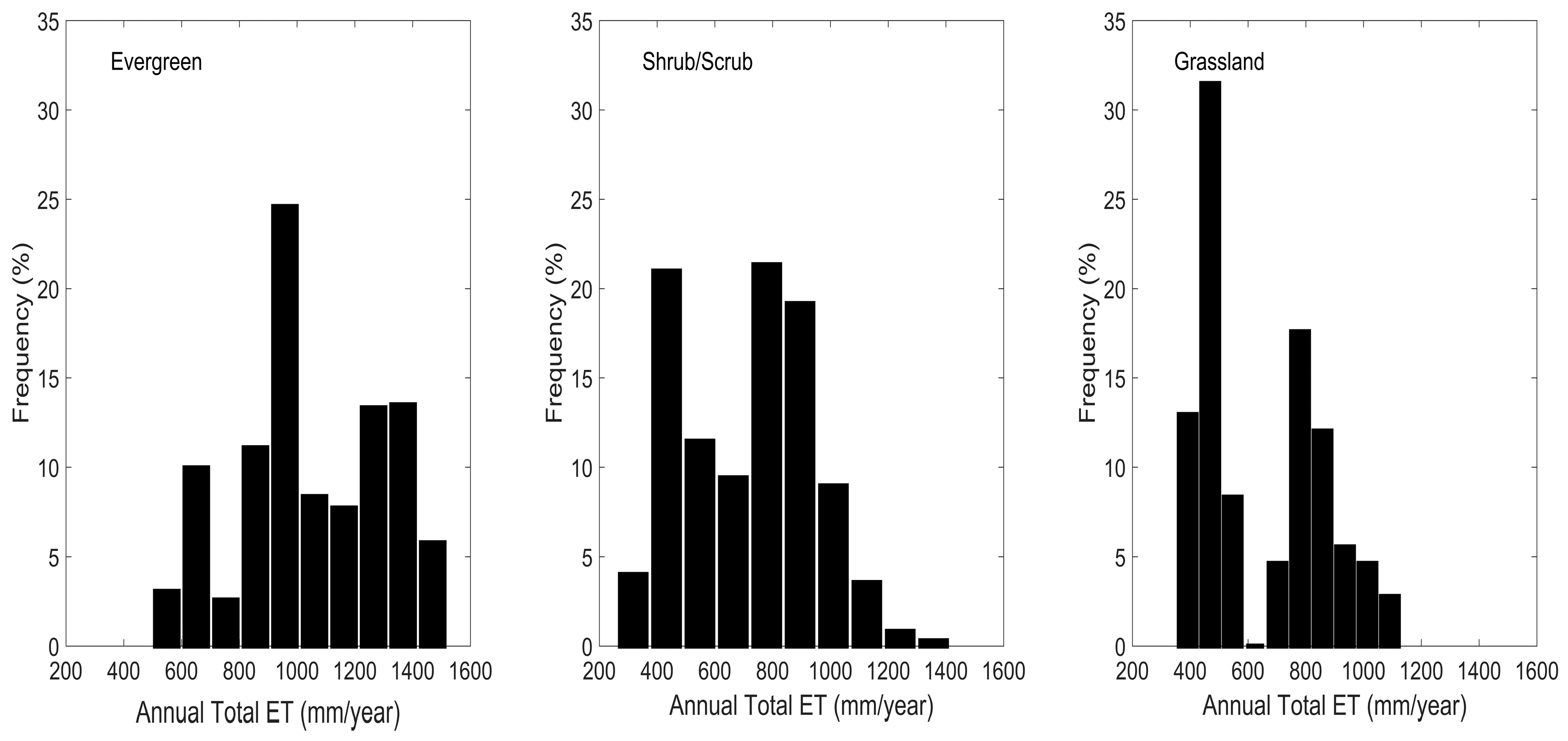
5.1. Annual Total Actual Evapotranspiration Estimates
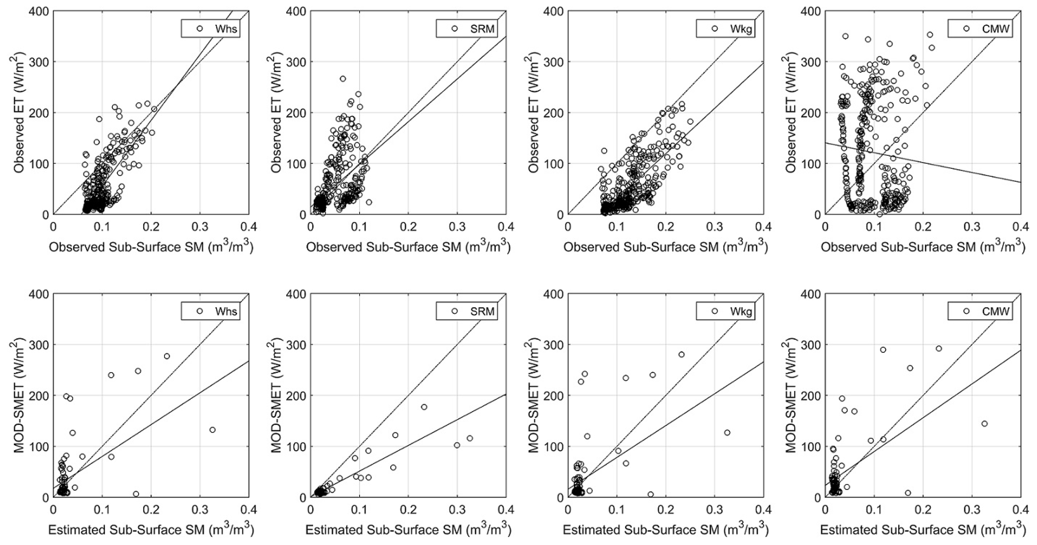
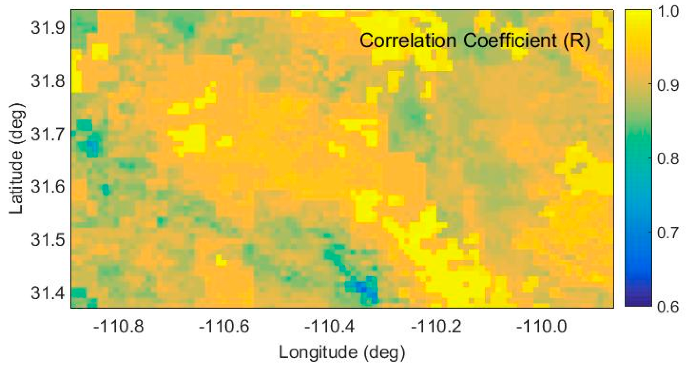
5.2. Soil Moisture Analysis
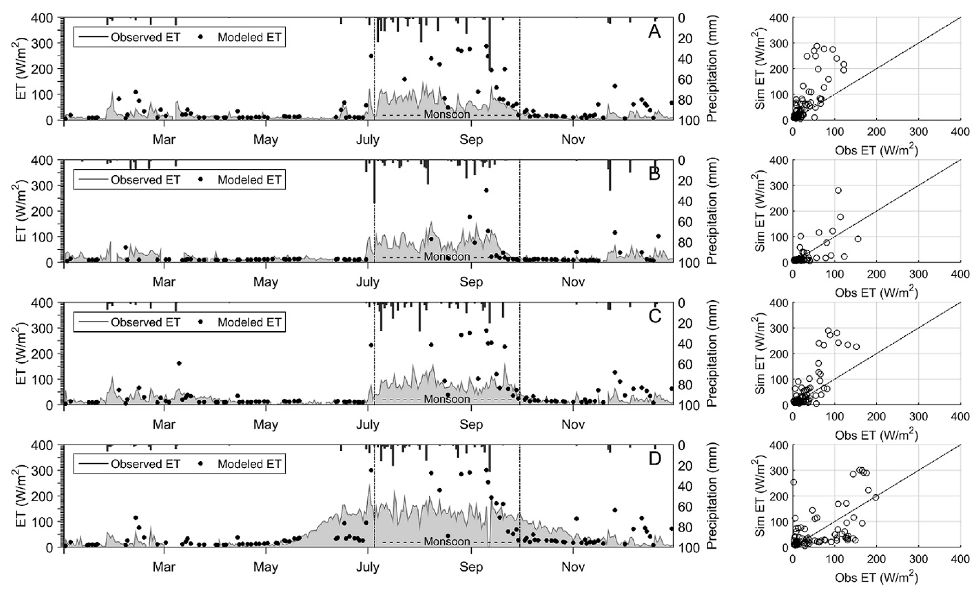
5.3. Validation
5.3.1. Ground-Based Observations
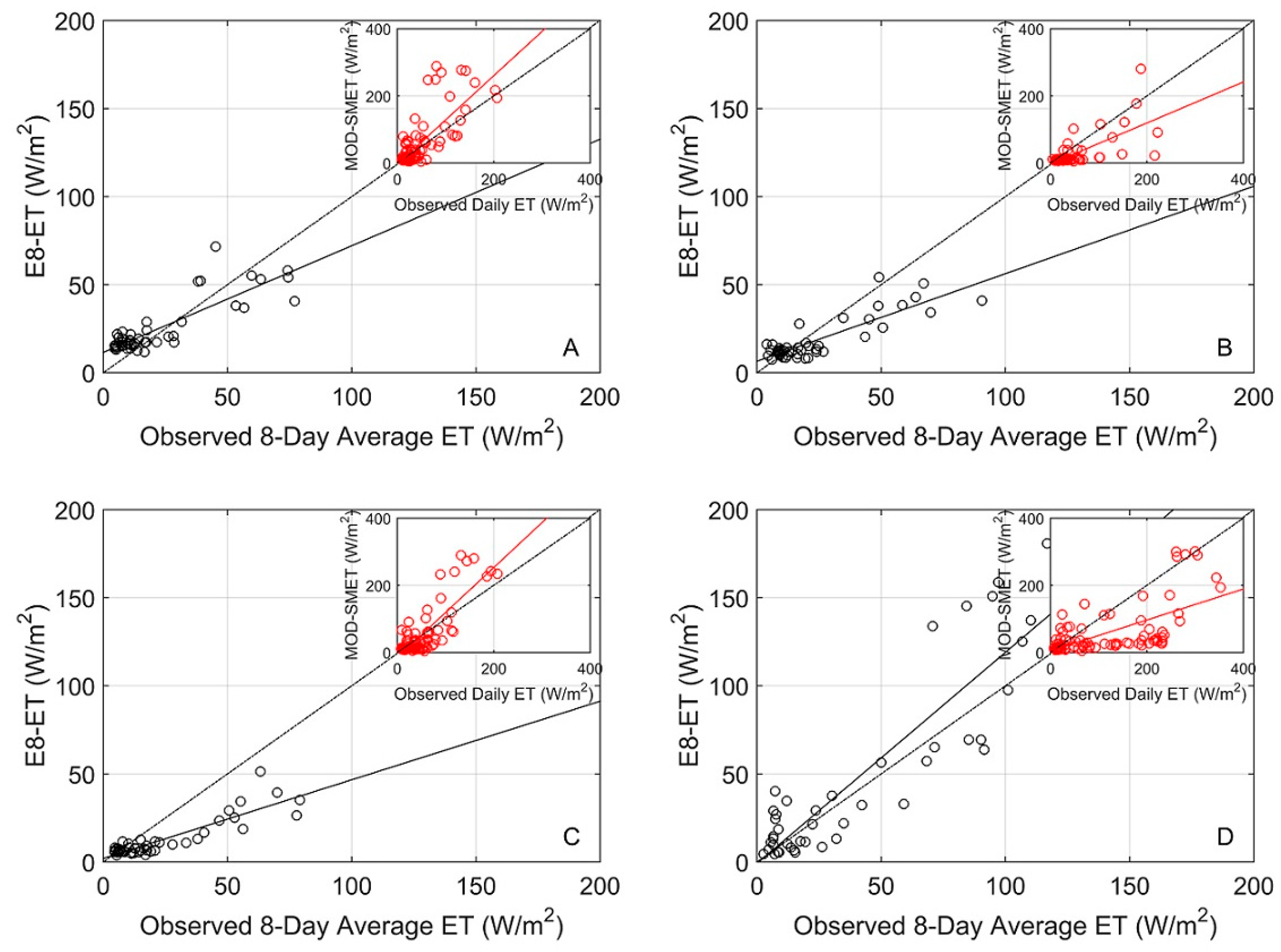
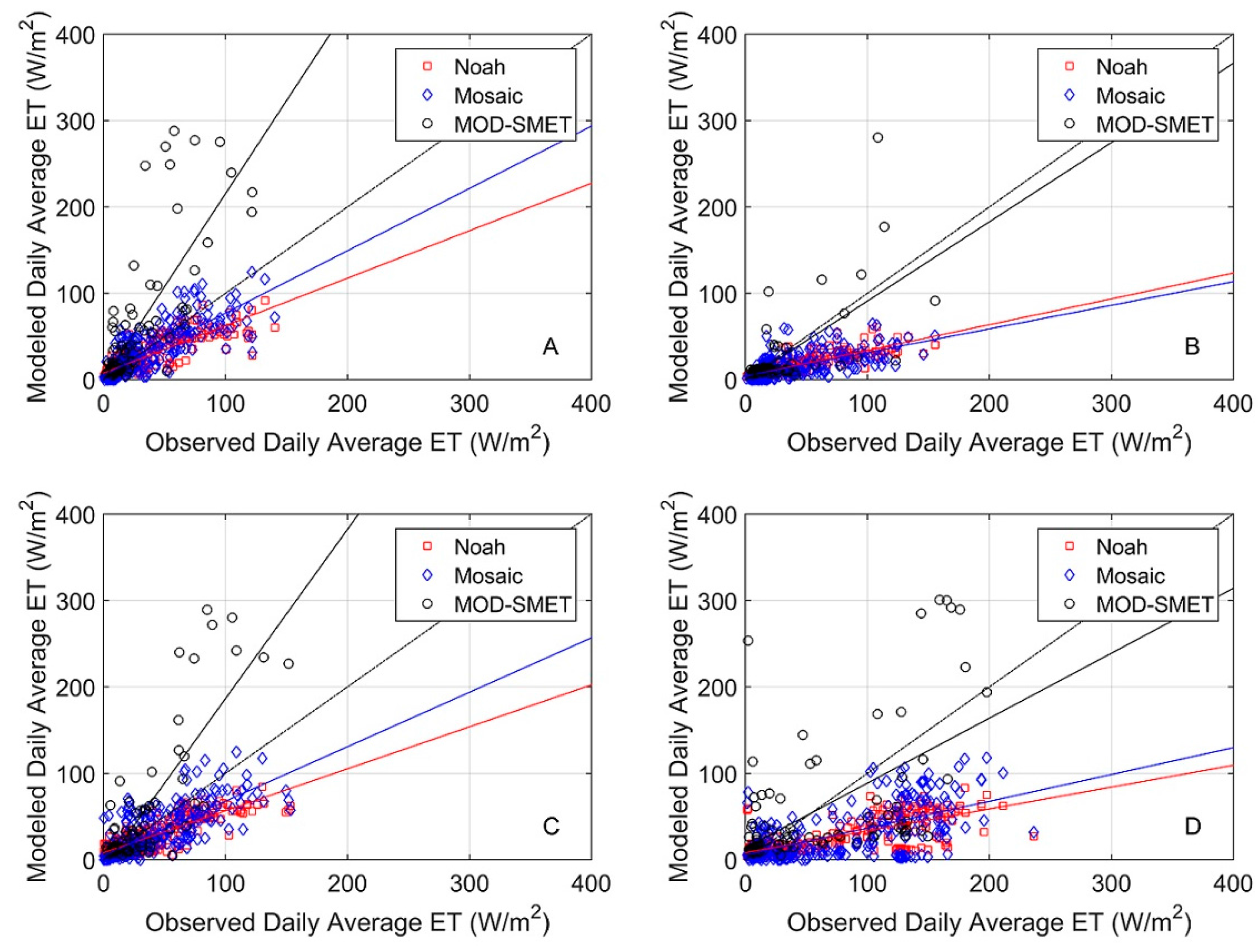
5.3.2. Eight-Day Empirical and NLDAS-2 Model Comparison
6. Conclusions
Acknowledgments
Author Contributions
Conflicts of Interest
References
- Sun, G.; Alstad, K.; Chen, J.; Chen, S.; Ford, C.R.; Lin, G.; Liu, C.; Lu, N.; McNulty, S.G.; Miao, H.; et al. A general predictive model for estimating monthly ecosystem evapotranspiration. Ecohydrology 2011, 4, 245–255. [Google Scholar] [CrossRef]
- Tang, R.; Li, Z.; Tang, B. An application of the Ts-VI triangle method with enhanced edges determination for evapotranspiration from MODIS data in arid and semi-arid regions: implementation and validation. Remote Sens. Environ. 2010, 114, 540–551. [Google Scholar] [CrossRef]
- Xu, C.Y.; Singh, V.P. Evaluation of three complimentary relationship evapotranspiration models by water balance approach to estimate actual regional evapotranspiration in different climate regions. J. Hydrol. 2005, 308, 105–121. [Google Scholar] [CrossRef]
- Kim, J.Y.; Hogue, T.S. Evaluation of a MODIS triangle-based evapotranspiration algorithm for semi-arid regions. J. Appl. Remote Sens. 2013, 7, 073493. [Google Scholar] [CrossRef]
- Schmid, H.P.; Lloyd, C.R. Spatial representativeness and the location bias of flux footprints over inhomogenous areas. Agric. For. Meteorol. 1999, 93, 195–209. [Google Scholar] [CrossRef]
- Chen, B.; Chen, J.M.; Mo, G.; Black, T.A.; Worthy, D.E.J. Comparison of regional carbon flux estimates from CO2 concentration measurements and remote sensing based footprint integration. Glob. Biogeochem. Cycles 2008, 22. [Google Scholar] [CrossRef]
- Courault, D.; Seguin, B.; Olioso, A. Review on estimation of evapotranspiration from remote sensing data: From empirical to numerical modeling approaches. Irrig. Drain. Syst. 2005, 19, 223–249. [Google Scholar] [CrossRef]
- Bastiaanssen, W.G.M.; Menenti, M.; Feddes, R.A.; Holtslag, A.A.M. A remote sensing surface energy balance algorithm for land (SEBAL) 1. Formulation. J. Hydrol. 1998, 212–213, 198–212. [Google Scholar] [CrossRef]
- Bastiaanssen, W.G.M.; Pelgrum, H.; Wang, J.; Ma, Y.; Moreno, J.F.; Roerink, G.J.; van der Wal, T. A Surface Energy Balance Algorithm for Land (SEBAL): Part 2 validation. J. Hydrol. 1998, 212–213, 213–229. [Google Scholar] [CrossRef]
- Bastiaanssen, W.G.M. SEBAL-based sensible and latent heat fluxes in the irrigated Gediz Basin, Turkey. J. Hydrol. 2000, 229, 87–100. [Google Scholar] [CrossRef]
- Allen, R.; Tasumi, M.; Morse, A.; Trezza, R.; Wright, J.; Bastiaanssen, W.; Lorite, I.; Robison, C. Satellite-based energy balance for Mapping Evapotranspiration with Internalized Calibration (METRIC)—Applications. J. Irrig. Drain. Eng. 2007, 133, 395–406. [Google Scholar] [CrossRef]
- Anderson, M.C.; Norman, J.M.; Mecikalski, J.R.; Otkin, J.A.; Kustas, W.P. A Climatological Study of Evapotranspiration and Moisture Stress across the Continental United States: 1. Model Formulation. J. Geophys. Res. 2007, 112, D10117. [Google Scholar] [CrossRef]
- Senay, G.B.; Budde, M.; Verdin, J.P.; Melesse, A.M. A coupled remote sensing and simplified surface energy balance approach to estimate actual evapotranspiration from irrigated fields. Sensors 2007, 7, 979–1000. [Google Scholar] [CrossRef]
- Senay, G.B.; Bohms, S.; Singh, R.K.; Gowda, P.H.; Velpuri, N.M.; Alemu, H.; Verdin, J.P. Operational evapotranspiration mapping using remote sensing and weather datasets: A new parameterization for the SSEB approach. J. Am. Water Resour. Assoc. 2013, 49, 577–591. [Google Scholar] [CrossRef]
- Carlson, T.N.; Gillies, R.R.; Perry, E.M. A method to make use of thermal infrared temperature and NDVI measurements to infer surface soil water content and fractional vegetation cover. Int. J. Remote Sens. 1994, 9, 161–173. [Google Scholar] [CrossRef]
- Jiang, L.; Islam, S. A methodology for estimation of surface evapotranspiration over large areas using remote sensing observations. Geophys. Res. Lett. 1999, 26, 2773–2776. [Google Scholar] [CrossRef]
- Jiang, L.; Islam, S. Estimation of surface evapotranspiration map over Southern Great Plains using remote sensing data. Water Resour. Res. 2001, 37, 329–340. [Google Scholar] [CrossRef]
- Jiang, L.; Islam, S. An intercomparison of regional latent heat flux estimation using remote sensing data. Int. J. Remote Sens. 2003, 24, 2221–2236. [Google Scholar] [CrossRef]
- Wang, K.; Li, Z.; Cribb, M. Estimation of evaporative fraction from a combination of day and night land surface temperature and NDVI: A new method to determine the Priestly-Taylor parameter. Remote Sens. Environ. 2006, 102, 293–305. [Google Scholar] [CrossRef]
- Bastiaanssen, W.G.M.; Noordman, E.; Pelgrum, H.; Davids, G.; Thoreson, B.; Allen, R. SEBAL model with remotely sensed data to improve water-resources management under actual field conditions. ASCE J. Irrig. Drain. Eng. 2005, 131, 85–93. [Google Scholar] [CrossRef]
- Singh, R.K.; Irmak, A.; Irmak, S.; Martin, D.L. Application of SEBAL model for mapping evapotranspiration and estimating surface energy fluxes in south-central Nebraska. J. Irrig. Drain. Eng. 2008, 134, 273–285. [Google Scholar] [CrossRef]
- Al Zayed, I.; Elagib, N.; Ribbe, L.; Heinrich, J. Satellite-based evapotranspiration over Gezira irrigation scheme, Sudan: A comparative study. Agric. Water Manag. 2016, 177, 66–76. [Google Scholar] [CrossRef]
- Lubczynski, M.W.; Gurwin, J. Integration of various data sources for transient groundwater modeling with spatio-temporally variable fluxes: Sardon study case, Spain. J. Hydrol. 2005, 306, 71–96. [Google Scholar] [CrossRef]
- Timmermans, W.J.; Meijerink, A.M.J. Remotely sensed actual evapotranspiration: Implications for groundwater management in Botswana. Int. J. Appl. Earth Obs. Geoinf. 1999, 1, 222–233. [Google Scholar] [CrossRef]
- Van der Kwast, J.; Timmermans, W.; Gieske, A.; Su, Z.; Olioso, A.; Jia, L.; Elbers, J.; Karssenberg, D.; de Jong, S. Evaluation of the Surface Energy Balance System (SEBS) applied to ASTER imagery with flux-measurements at the SPARC 2004 site (Barrax, Spain). Hydrol. Earth Syst. Sci. 2009, 13, 1337–1347. [Google Scholar] [CrossRef]
- Feddes, R.A.; Kowalik, P.J.; Zaradny, H. Simulation of Field Water Use and Crop Yield; Centre for Agricultural Publishing and Documentation: Wageningen, The Netherlands, 1978. [Google Scholar]
- Belmans, J.G.; Wesseling, J.; Feddes, R.A. Simulation of the water balance of a cropped soil, SWATRE. J. Hydrol. 1983, 63, 271–286. [Google Scholar] [CrossRef]
- Wagenet, R.J.; Hutson, J.L. Scale-Dependency of solute transport modeling/GIS applications. J. Environ. Qual. 1996, 25, 499–510. [Google Scholar] [CrossRef]
- Hain, C.R.; Mecikalski, J.R.; Anderson, M.C. Retrieval of an available water-based soil moisture proxy from thermal infrared remote sensing. Part I: methodology and validation. J. Hydrometeorol. 2009, 10, 665–683. [Google Scholar]
- Hain, C.R.; Crow, W.T.; Mecikalski, J.R.; Anderson, M.C.; Holmes, T. An intercomparison of available soil moisture estimates from thermal infrared and passive microwave remote sensing and land surface modeling. J. Geophys. Res. 2011, 116, D15107. [Google Scholar] [CrossRef]
- Mahfouf, J.F.; Noilhan, J. Comparative study of various formulations of evaporation from bare soil using in situ data. J. Appl. Meteorol. 1991, 30, 1354–1365. [Google Scholar] [CrossRef]
- Mahrt, L.; Pan, H.L. A two layer model for soil hydrology. Bound. Layer Meteorol. 1984, 29, 1–20. [Google Scholar] [CrossRef]
- Campbell, G.S.; Norman, J.M. An Introduction to Environmental Biophysics; Springer: New York, NY, USA, 1998. [Google Scholar]
- Chen, F.; Mitchell, K.; Schaake, J.; Xue, Y.; Pan, H.L.; Koren, V.; Duan, Q.Y.; Ek, M. Modeling of land surface evaporation by four schemes and comparison with FIFE observations. J. Geophys. Res. 1996, 101, 7251–7268. [Google Scholar] [CrossRef]
- Betts, A.K.; Chen, F.; Mitchell, K.E.; Janjic, Z.I. Assessment of the land surface and boundary layer models in two operational versions of the NCEP Eta model using FIFE data. Mon. Weather Rev. 1997, 125, 2896–2916. [Google Scholar] [CrossRef]
- Song, J.; Wesely, M.L.; Coulter, R.L.; Brandes, E.A. Estimating watershed evapotranspiration with PASS. Part I: Inferring root-zone moisture conditions using satellite data. J. Hydrometeorol. 2000, 1, 447–461. [Google Scholar] [CrossRef]
- Gokmen, M.; Vekerdy, Z.; Verhoef, A.; Verhoef, W.; Batelaan, O.; van der Tol, C. Integration of soil moisture in SEBS for improving evapotranspiration estimation under water stress conditions. Remote Sens. Environ. 2012, 121, 261–274. [Google Scholar] [CrossRef]
- Bastiaanssen, W.G.M.; Cheema, M.J.M.; Immerzeel, W.W.; Miltenburg, I.J.; Pelgrum, H. Surface energy balance and actual evapotranspiration of the transboundary Indus Basin estimated from satellite measurements and the ETLook model. Water Resour. Res. 2012, 48. [Google Scholar] [CrossRef]
- Miralles, D.G.; Holmes, T.R.H.; De Jeu, R.A.M.; Gash, J.H.; Meesters, A.G.C.A.; Dolman, A.J. Global land-surface evaporation estimated from satellite-based observations. Hydrol. Earth Syst. Sci. 2011, 15, 453–469. [Google Scholar] [CrossRef] [Green Version]
- Choi, M.; Kim, T.W.; Kustas, W.P. Reliable estimation of evapotranspiration on agricultural fields predicted by the Priestley-Taylor model using soil moisture data from ground and remote sensing observations compared with the Common Land Model. Inter. J. Remote Sens. 2011, 32, 4571–4587. [Google Scholar] [CrossRef]
- Kim, J.; Hogue, T.S. Evaluation of a MODIS-based potential evapotranspiration product at the point scale. J. Hydrometeorol. 2008, 9, 444–460. [Google Scholar] [CrossRef]
- Chauhan, N.; Miller, S.; Ardanuy, P. Spaceborne soil moisture estimation at high resolution: a microwave-optical/IR synergistic approach. Inter. J. Remote Sens. 2003, 22, 4599–4622. [Google Scholar] [CrossRef]
- Hemakumara, M.; Kalma, J.; Walker, J.; Willgoose, G. Downscaling of low resolution passive microwave soil moisture observations. In 2nd International CAHMDA Workshop on the Terrestrial Water Cycle: Modelling and Data Assimilation across Catchment Scales; Teuling, A.J., Ed.; Wegeningen University: Wageningen, The Netherlands, 2004; pp. 67–71. [Google Scholar]
- Hossain, A.; Easson, G. Evaluating the potential of VI-LST triangle model for quantitative estimation of soil moisture using optical imagery. In Proceedings of the IEEE International Geoscience and Remote Sensing Symposium, Boston, MA, USA, 7–11 July 2008.
- Scott, R.L.; Cable, W.L.; Huxman, T.E.; Nagler, P.L.; Hernandez, M.; Goodrich, D.C. Multiyear riparian evapotranspiration and groundwater use for a semiarid watershed. J. Arid Environ. 2008, 72, 1232–1246. [Google Scholar] [CrossRef]
- Bunting, D.P.; Kurc, S.A.; Glenn, E.P.; Nagler, P.L.; Scott, R.L. Insights for empirically modeling evapotranspiration influenced by riparian and upland vegetation in semiarid regions. J. Arid Environ. 2014, 111, 42–52. [Google Scholar] [CrossRef]
- Homer, C.G.; Dewitz, J.A.; Yang, L.; Jin, S.; Danielson, P.; Xian, G.; Coulston, J.; Herold, N.D.; Wickman, J.D.; Megown, K. Completion of the 2011 National Land Cover Database for the conterminous United States-representing a decade of land cover change information. Photogramm. Eng. Remote Sens. 2015, 81, 345–354. [Google Scholar]
- Adams, D.K.; Comrie, A.C. The North American Monsoon. Bull. Am. Meteorol. Soc. 1997, 78, 2197–2213. [Google Scholar] [CrossRef]
- National Weather Service Forecast Office. Rainfall across Southeast Arizona during 2013 Monsoon. Available online: http:www.wrh.noaa.gov/twc/monsoon/season/2013monsoon.php (accessed on 6 January 2016).
- Scott, R.L.; Huxman, T.E.; Cable, W.L.; Emmerich, W.E. Partitioning of evapotranspiration and its relation to carbon dioxide exchange in a Chihuahuan Desert shrubland. Hydrol. Process. 2006, 20, 3227–3243. [Google Scholar] [CrossRef]
- Scott, R.L. Using watershed water balance to evaluate the accuracy of eddy covariance evapotranspiration measurements for three semiarid ecosystems. Agric. For. Meteorol. 2010, 150, 219–225. [Google Scholar] [CrossRef]
- Kurc, S.A.; Benton, L.M. Digital image-derived greenness links deep soil moisture to carbon uptake in a creosotebush-dominated shrubland. J. Arid Environ. 2010, 74, 585–594. [Google Scholar] [CrossRef]
- Scott, R.L.; Edwards, E.A.; Shuttleworth, W.J.; Huxman, T.E.; Watts, C.; Goodrich, D.C. Interannual and seasonal variation in fluxes of water and carbon dioxide from a riparian woodland ecosystem. Agric. For. Meteorol. 2004, 122, 65–84. [Google Scholar] [CrossRef]
- Glenn, E.P.; Scott, R.L.; Nguyen, U.; Nagler, P.L. Wide-area ratios of evapotranspiration to precipitation in monsoon-dependent semiarid vegetation communities. J. Arid. Environ. 2015, 117, 84–95. [Google Scholar] [CrossRef]
- Twine, T.E.; Kustas, W.P.; Norman, J.M.; Cook, D.R.; Houser, P.R.; Meyers, T.P.; Prueger, J.H.; Starks, P.J.; Wesely, M.L. Correcting eddy-covariance flux under- estimates over a grassland. Agric. For. Meteorol. 2000, 103, 279–300. [Google Scholar] [CrossRef]
- Scott, R.L.; Jenerette, G.D.; Potts, D.L.; Huxman, T.E. Effects of seasonal drought on net carbon dioxide exchange from a woody-plant-encroached semiarid grassland. J. Geophys. Res. 2009, 114. [Google Scholar] [CrossRef]
- Kerr, Y.H.; Waldteufel, P.; Wigneron, J.P.; Martinuzzi, J.; Font, J.; Berger, M. Soil moisture retrieval from space: The Soil Moisture and Ocean Salinity (SMOS) mission. IEEE Trans. Geosci. Remote Sens. 2001, 39, 1729–1735. [Google Scholar] [CrossRef]
- Kerr, Y.H.; Waldteufel, P.; Wigneron, J.P.; Delwart, S.; Cabot, F.; Boutin, J.; Escorihuela, M.; Font, J.; Reul, N.; Gruhier, C.; et al. The SMOS Mission: New tool for monitoring key elements of the global water cycle. IEEE Trans. Geosci. Remote Sens. 2010, 98, 666–687. [Google Scholar] [CrossRef] [Green Version]
- Schmugge, T.; Jackson, T. Mapping surface soil moisture with microwave radiometers. Meteorol. Atmos. Phys. 1994, 54, 213–223. [Google Scholar] [CrossRef]
- Jackson, T.; Schmugge, T. Passive microwave remote sensing system for soil moisture: Some supporting research. IEEE Trans. Geosci. Remote Sens. 1989, 27, 225–235. [Google Scholar] [CrossRef]
- Jackson, T.; Schmugge, T. Vegetation effects on the microwave emission from soils. Remote Sens. Environ. 2001, 36, 203–212. [Google Scholar] [CrossRef]
- Escorihuela, M.J.; Chanzy, A.; Wigneron, J.P.; Kerr, Y.H. Effective soil moisture sampling depth of L-band radiometry: A case study. Remote Sens. Environ. 2010, 114, 995–1001. [Google Scholar] [CrossRef] [Green Version]
- Knipper, K.; Hogue, T.; Scott, R.; Franz, K. Downscaling AMSR2 and SMOS soil moisture with MODIS visible and infrared products over southern Arizona. J. Appl. Remote Sens. 2017, in press. [Google Scholar]
- Kerr, Y.H.; Waldteufel, P.; Richaume, P.; Wigneron, J.P.; Ferrazzoli, P.; Mahmoodi, A.; Bitar, A.A.; Cabot, F.; Gruhier, C.; Juglea, S.E.; et al. The SMOS soil moisture retrieval algorithm. IEEE Trans. Geosci. Remote Sens. 2012, 50, 1384–1403. [Google Scholar] [CrossRef]
- Hornbuckle, B.; England, A. Diurnal variation of vertical temperature gradients within a field of maize: Implications for satellite microwave radiometry. IEEE Geosci. Remote Sens. Lett. 2005, 2, 74–77. [Google Scholar] [CrossRef]
- Entekhabi, D.; Njoku, E.; O’Neill, P.; Kellogg, K.; Crow, W.; Edelstein, W.; Entin, J.; Goodman, S.; Jackson, T.; Johnson, J.; et al. The soil moisture active passive SMAP mission. Proc. IEEE 2010, 98, 704–716. [Google Scholar] [CrossRef]
- Huete, A.R.; Didan, K.; van Leeuwen, W.J.D.; Vermote, E.F. Global-scale analysis of vegetation indices for moderate resolution monitoring of terrestrial vegetation. Proc. SPIE 1999. [Google Scholar] [CrossRef]
- Murray, R.S.; Nagler, P.L.; Morino, K.; Glenn, E.P. An Empirical algorithm for estimating agricultural and riparian evapotranspiration using MODIS enhanced vegetation index and ground measurements of ET. II. Application to the Lower Colorado River, US. Remote Sens. 2009, 1, 1125–1138. [Google Scholar] [CrossRef]
- Nagler, P.; Cleverly, J.; Lampkin, D.; Glenn, E.; Huete, A.; Wan, Z. Predicting riparian evapotranspiration from MODIS vegetation indices and meteorological data. Remote Sens. Environ. 2005, 94, 17–30. [Google Scholar] [CrossRef]
- Nagler, P.; Scott, R.; Westenberg, C.; Cleverly, J.; Glenn, E.; Huete, A. Evapotranspiration on western U.S. rivers estimated using the enhanced vegetation index from MODIS and data from eddy covariance and bowen ratio flux towers. Remote Sens. Environ. 2005, 97, 337–351. [Google Scholar] [CrossRef]
- Nagler, P.L.; Glenn, E.P.; Kim, H.; Emmerich, W.; Scott, R.L.; Huxman, T.E.; Huete, A.R. Relationship between evapotranspiration and precipitation pulses in semiarid rangeland estimated by soil moisture flux towers and MODIS vegetation indices. J. Arid Environ. 2007, 70. [Google Scholar] [CrossRef]
- Liang, X.; Lettenmaier, D.P.; Wood, E.F.; Burges, S.J. A simple hydrologically based model of land surface water and energy fluxes for GCMs. J. Geophys. Res. 1994, 99, 415–428. [Google Scholar] [CrossRef]
- Koster, R.; Suarez, M. The components of a SVAT scheme and their effects on a GCM’s hydrological cycle. Adv. Water Resour. 1994, 17, 61–78. [Google Scholar] [CrossRef]
- Burnash, R.J.; Ferral, R.L.; McGuire, R.A. A Generalized Streamflow Simulation System Conceptual: Modeling for Digital Computers; Joint Federal-State River Forecast Center: Sacramento, CA, USA, 1973. [Google Scholar]
- Xia, Y.; Mitchell, K.; Ek, M.; Sheffield, J.; Cosgrove, B.; Wood, E.; Luo, L.; Alonge, C.; Wei, H.; Meng, J.; et al. Continental-scale water and energy flux analysis and validation for the North American Land Data Assimilation System project phase 2 (NLDAS-2): 1. Comparison analysis and application of model products. J. Geophys. Res. 2012, 117. [Google Scholar] [CrossRef]
- Xia, Y.; Mitchell, K.; Ek, M.; Cosgrove, B.; Sheffield, J.; Luo, L.; Alonge, C.; Wei, H.; Meng, J.; Livneh, B.; et al. Continental-scale water and energy flux analysis and validation for the North American Land Data Assimilation System project phase 2 (NLDAS-2): 2. Validation of model simulated streamflow. J. Geophys. Res. 2012, 117. [Google Scholar] [CrossRef]
- Priestley, C.H.B.; Taylor, R.J. On the assessment of surface heat flux and evaporation using large scale parameters. Mon. Weather Rev. 1972, 100, 81–92. [Google Scholar] [CrossRef]
- Flint, A.L.; Childs, S.W. Use of the Priestley–Taylor evaporation equation for soil–water limited conditions in a small forest clear-cut. Agric. For. Meteorol. 1991, 56, 247–260. [Google Scholar] [CrossRef]
- Stannard, D.I. Comparison of Penman–Monteith, Shuttleworth–Wallace, and modified Priestley–Taylor evapotranspiration models for wildland vegetation in semiarid rangeland. Water Resour. Res. 1993, 29, 1379–1392. [Google Scholar] [CrossRef]
- Sumner, D.M. Evapotranspiration from Successional Vegetation in a Deforested Area of the Lake Wales Ridge, Florida; U.S. Geological Survey Water-Resources Investigations Report 96-4244; U.S. Department of Interior, U.S. Geological Survey: Tallahassee, FL, USA, 1996.
- Pereira, A.R.; Nova, N.A.V. Analysis of the Priestley–Taylor parameter. Agric. For. Meteorol. 1992, 61, 1–9. [Google Scholar] [CrossRef]
- Fisher, J.B.; Debise, T.A.; Qi, Y.; Xu, M.; Godlstein, A.H. Evapotranspiration models compared on a Sierra Nevada forest ecosystem. Model. Softw. 2005, 20, 783–796. [Google Scholar] [CrossRef]
- Zillman, J.W. A Study of Some Aspects of the Radiation and Heat Budgets of the Southern Hemisphere Oceans; Australian Government Publishing Service: Canberra, Australia, 1972.
- Bisht, G.; Bras, R.L. Estimation of net radiation from the MODIS data under all sky conditions: Southern Great Plains case study. Remote Sens. Environ. 2010, 114, 1522–1534. [Google Scholar] [CrossRef]
- Niemela, S.; Raisanen, P.; Savijarvi, H. Comparison of surface radiative flux parameterizations: Part I: Longwave radiation. Atmos. Res. 2001, 58, 1–18. [Google Scholar] [CrossRef]
- Bisht, G.; Venturini, V.; Islam, S.; Jiang, L. Estimation of the net radiation using MODIS (Moderate Resolution Imaging Spectroradiometer) data for clear sky days. Remote Sens. Environ. 2005, 97, 52–67. [Google Scholar] [CrossRef]
- Brutsaert, W. One derivable formula for long-wave radiation from clear skies. Water Resour. Res. 1975, 11, 742–744. [Google Scholar] [CrossRef]
- Liu, Y.Y.; Parinussa, R.M.; Dorigo, W.A.; de Jeu, R.A.M.; Wagner, W.; Van Dijk, A.I.J.M. Developing an improved soilmoisture dataset by blending passive and active microwave satellite-based retrievals. Hydrol. Earth Syst. Sci. 2011, 15, 425–436. [Google Scholar] [CrossRef] [Green Version]
- Piles, M.; Camps, A.; Vall-llossera, M.; Corbella, I.; Panciera, R.; Rudiger, C.; Kerr, Y.H.; Walker, J. Downscaling SMOS-derived soil moisture using MODIS Visible/Infrared. IEEE Trans. Geosci. Remote Sens. 2011, 49, 3156–3166. [Google Scholar] [CrossRef]
- Kim, J.; Hogue, T. Improving spatial soil moisture representation through integration of AMSR-E and MODIS products. IEEE T. Geosci. Remote Sens. 2012, 50, 446–460. [Google Scholar] [CrossRef]
- Saxton, K.E.; Rawls, W.J.; Romberger, J.S.; Papendick, R.I. Estimating generalized soil-water characteristics from texture. Soil Sci. Soc. Am. J. 1986, 50, 1031–1036. [Google Scholar] [CrossRef]
- Brooks, R.J.; Corey, A.T. Hydraulic Properties of Porous Media; Hydrology Papers No. 3; Colorado State University: Fort Collins, CO, USA, 1996; Volume 3. [Google Scholar]
- Van Genuchten, M.T. A closed-form equation for predicating the hydraulic conductivity on unsaturated soils. Soil Sci. Soc. Am. J. 1980, 44, 892–898. [Google Scholar] [CrossRef]
- Singh, R.K.; Senay, G.B.; Velpuri, N.M.; Bohms, S.; Scott, R.L.; Verdin, J.P. Actual evapotranspiration (water use) assessment of the Colorado River Basin at the Landsat resolution using the Operational Simplified Surface Energy Balance Model. Remote Sens. 2014, 6, 233–256. [Google Scholar] [CrossRef]
- Kurc, S.A.; Small, E.E. Soil moisture variations and ecosystem-scale fluxes of water and carbon in semiarid grassland and shrubland. Water Resour. Res. 2007, 43. [Google Scholar] [CrossRef]
- Williams, D.G.; Scott, R.L.; Huxman, T.E.; Goodrich, D.C.; Lin, G. Sensitivity of riparian ecosystems to moisture pulses in semiarid environments. Hydrol. Process. 2006, 20, 3191–3205. [Google Scholar] [CrossRef]
- Goodrich, D.C.; Unkrich, C.L.; Keefer, T.O.; Nichols, M.H.; Stone, J.J.; Levick, L.R.; Scott, R.L. Event to multidecadal persistence in rainfall and runoff in southeast Arizona. Water Resour. Res. 2008, 44. [Google Scholar] [CrossRef]
- Cox, J.R.; Frasier, G.W.; Renard, K.G. Biomass distribution at grassland and shrubland sites. Rangelands 1986, 8, 67–69. [Google Scholar]
- Crow, W.T. Impact of soil moisture aggregation on surface energy flux prediction during SGP’9. Geophys. Res. Lett. 2002, 29. [Google Scholar] [CrossRef]
- He, L.; Ivanov, V.Y.; Bohrer, G.; Maurer, K.D.; Vogel, C.S.; Moghaddam, M. Effects of fine-scale soil moisture and canopy heterogeneity on energy and water fluxes in a northern temperate mixed forest. Agric. For. Meteorol. 2014, 184, 243–256. [Google Scholar] [CrossRef]
- Ronda, R.J.; van den Hurk, B.J.J.M.; Holtslag, A.A.M. Spatial heterogeneity of the soil moisture content and its impact on surface flux densities and near-surface meteorology. J. Hydrometeorol. 2002, 3, 556–570. [Google Scholar] [CrossRef]
- Tang, R.; Li, Z.L.; Chen, K.S. Validating MODIS-derived land surface evapotranspiration with in situ measurements at two Ameriflux sites in a semiarid regions. J. Geophys. Res. 2011, 116. [Google Scholar] [CrossRef]


| Site | Digital Object Identifier (DOI) | Latitude (deg) | Longitude (deg) | Measurement Height (m) | Land Cover |
|---|---|---|---|---|---|
| Lucky Hills (Whs) | 10.17190/AMF/1246113 | 31.749 | −110.052 | 6.4 | Open Shrublands |
| Santa Rita–Mesquite (SRM) | 10.17190/AMF/1246104 | 31.822 | −110.867 | 7.8 | Woody Savannas |
| Charleston–Mesquite (CMW) | NA | 31.664 | −110.178 | 14.0 | Riparian Woodland |
| Kendall Grassland (Wkg) | 10.17190/AMF/1246112 | 31.738 | −109.943 | 6.4 | Grassland |
| Land Use/Land Cover | Mean Annual ET (mm) | Standard Deviation (mm) |
|---|---|---|
| Evergreen Forest | 1050 | 248 |
| Shrub/Scrub | 713 | 224 |
| Grassland | 647 | 210 |
| Model | SITE | R (-) | RMSE (W/m2) | Bias (W/m2) | Slope (-) | Intercept (W/m2) |
|---|---|---|---|---|---|---|
| MOD-SMET | Whs | 0.77 | 49.0 | 10.0 | 1.32 | −3.50 |
| SRM | 0.69 | 40.0 | −20.0 | 0.61 | −2.84 | |
| Wkg | 0.83 | 40.0 | 0.6 | 1.34 | −15.0 | |
| CMW | 0.63 | 96.0 | −56.0 | 0.46 | 4.4 | |
| Eight-Day Empirical Model | Whs | 0.85 | 11.8 | 2.8 | 0.61 | 11.6 |
| SRM | 0.86 | 13.2 | −5.3 | 0.62 | 10.6 | |
| Wkg | 0.89 | 16.6 | −10.7 | 0.45 | 2.0 | |
| CMW | 0.89 | 24.8 | 7.0 | 1.20 | −0.9 | |
| Noah | Whs | 0.86 | 18.0 | −5.5 | 0.55 | 7.7 |
| SRM | 0.86 | 31.0 | −20.0 | 0.30 | 4.0 | |
| Wkg | 0.85 | 21.0 | −9.7 | 0.49 | 8.1 | |
| CMW | 0.76 | 61.0 | −41.0 | 0.25 | 8.2 | |
| Mosaic | Whs | 0.83 | 17.0 | −3.2 | 0.72 | 5.0 |
| SRM | 0.66 | 33.0 | −21.0 | 0.27 | 4.2 | |
| Wkg | 0.78 | 22.0 | −8.1 | 0.63 | 4.7 | |
| CMW | 0.66 | 61.0 | −39.0 | 0.31 | 5.5 |
| Site | Tower ET (mm/year) | MOD-SMET (mm/year) | Noah (mm/year) | Mosaic (mm/year) | E8-ET (mm/year) |
|---|---|---|---|---|---|
| Whs | 359 (20) | 763 (50) | 292 (13) | 323 (17) | 281 (14) |
| SRM | 387 (22) | 395 (26) | 168 (7) | 160 (8) | 230 (8) |
| Wkg | 415 (21) | 750 (50) | 309 (12) | 323 (17) | 156 (7) |
| CMW | 763 (40) | 905 (55) | 297 (12) | 313 (18) | 562 (32) |
© 2017 by the authors. Licensee MDPI, Basel, Switzerland. This article is an open access article distributed under the terms and conditions of the Creative Commons Attribution (CC BY) license ( http://creativecommons.org/licenses/by/4.0/).
Share and Cite
Knipper, K.; Hogue, T.; Scott, R.; Franz, K. Evapotranspiration Estimates Derived Using Multi-Platform Remote Sensing in a Semiarid Region. Remote Sens. 2017, 9, 184. https://doi.org/10.3390/rs9030184
Knipper K, Hogue T, Scott R, Franz K. Evapotranspiration Estimates Derived Using Multi-Platform Remote Sensing in a Semiarid Region. Remote Sensing. 2017; 9(3):184. https://doi.org/10.3390/rs9030184
Chicago/Turabian StyleKnipper, Kyle, Terri Hogue, Russell Scott, and Kristie Franz. 2017. "Evapotranspiration Estimates Derived Using Multi-Platform Remote Sensing in a Semiarid Region" Remote Sensing 9, no. 3: 184. https://doi.org/10.3390/rs9030184