1. Introduction
Recent advances in Geomatics Science enable the use of a wide range of sensors to record, catalogue and analyze Cultural Heritage (CH) sites: from RGB and multispectral cameras [
1,
2] and Terrestrial Laser Scanner (TLS) [
3], to Ground Penetrating Radar (GPR) [
4] and Raman Spectroscopy [
5]. Furthermore, airborne LiDAR (Laser Imaging Detection and Ranging) is used as a remote sensing device for 3D surveying and modeling of extensive archaeological sites [
6,
7]. Nowadays, hybrid sensors such as Mobile LiDAR Systems (MLS) [
8,
9] bring added value to record large and complex sites. Although the most common solution based on MLS are boarded on vans and applied in the field of civil engineering and construction [
10], MLS has been useful in other fields, such as geology [
11]; agriculture, biology or forestry [
12,
13,
14]; and even in the inspection of high-voltage power lines [
15]. The last developments allow the use of MLS boarded in a backpack [
16] or even in autonomous robots [
17], offering a flexible solution in terms of accuracy, flexibility, point density and access to indoor and non-transitable areas [
18,
19,
20,
21,
22]. These specific solutions are still under development and several approaches are being experienced and tested [
23,
24].
MLS process and management optimization has become a key point. Even though MLS reduces extremely data collection phase, it still requires a lot of time and resources consumption to extract meaningful information [
25] and even more time for 3D modeling. At this point, and for large and unstructured point cloud, some authors [
26] showed that it is more efficient to carry out the simplification of the point cloud before creating a mesh. In terms of workflow optimization, it may be useful when the presence of particular characteristics (e.g., breaklines) is desirable [
27]. MLS optimization, understood not only as decimation but a smart filtering, has proven to be relevant in different fields, such as infrastructures management [
28], reverse engineering [
29], object detection [
30], object fitting [
31] and visualization optimization through Web services by means of mobile devices [
32].
It is a well-known fact that CH information systems such as Nubes Project [
33,
34] and Cultural Heritage Information System Projects [
35,
36,
37] become the basis for an effective management of CH. However, they are also extremely important for its dissemination and decision making. These Systems and Projects are usually based on 3D Web interfaces [
38]. Thus, it is clear that, in order to guarantee and improve the specific visualization requirements of 3D Web systems, the MLS complex geometric datasets need to be optimized.
Based on the remarks above, this paper aims to analyze the suitability of MLS for CH documentation and dissemination purposes from a two-fold approach. Firstly, an accuracy assessment is performed. For this purpose, the acquired MLS data were compared with a ground truth defined by a milimetric laser scanner point cloud. Secondly, the data suitability, in terms of 3D point cloud optimization for the data dissemination, is evaluated.
This manuscript is organized as follows. After the Introduction, sensors and devices are described in
Section 2. In
Section 3, the multi-sensor integration methodology and multi-data process workflow proposed are detailed. In
Section 4, the representative study case of the Medieval Wall of Avila (Spain) is shown. Finally, in
Section 5 and
Section 6, discussion and conclusions are respectively discoursed.
2. Materials
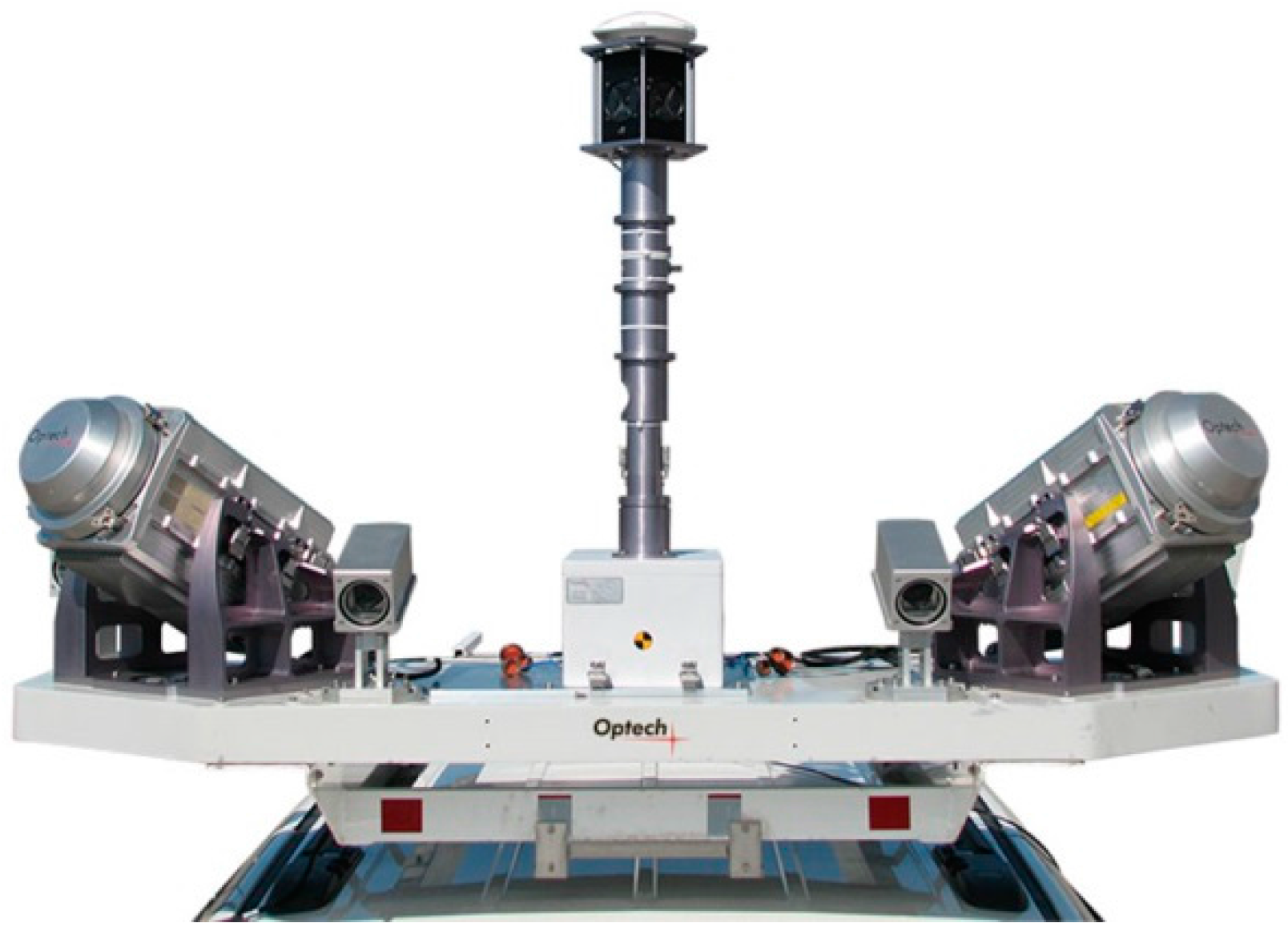
The evaluated mobile LiDAR technology is a LYNX Mobile Mapper manufactured by Optech (
Figure 1) [
9,
39]. This system is composed of two LiDAR sensors, four RGB cameras and an Applanix POS LV 520 IMU. The system is configured to take 500,000 points per second with a scan frequency of 200 Hz. The maximum range of the sensors is 200 m, with a precision of 8 mm (one sigma) and permission to obtain up to 4 echoes of the signal and the intensity reflected by the objects at a 1550 nm wavelength (
Table 1). Along with the geometric measurement system, the MLS incorporates a multisensory camera to acquire the radiometric texture of the scanned elements.
In this study, the MLS is mounted on a car, achieving speeds up to 40 km/h during the data capture.
The use of MLS is not completely straightforward. It requires an initial data acquisition plan, especially for the large cultural heritage sites. In this regard, any error in the INS will be directly propagated to the point cloud, being especially complicated in scenarios with the presence of narrow streets (e.g., urban CH sites), or dense vegetation, which could provide a loss in accuracy by the multi-path and occlusion of the GNSS signal [
40]. Besides, the boresight angles and level-arm (related to the MLS assembly), which are kept constant throughout the whole scanning process, require to be precisely determined to avoid any loss in the overall accuracy [
41]. To this end, some regular surfaces (e.g., road surface) should be measured prior to the data acquisition for its calibration. The most critical aspect in data acquisition planning is the boresight, which could cause that same scene acquisition in different trajectories to not overlap correctly. Additionally, the height of the CH buildings could be a limitation to the system due to the vertical angle, so those trajectories closer to the object should be avoided to reduce the occlusions in the final point cloud.
To assess the quality of the MLS, a Time-of-Flight (ToF) [
42,
43] TLS Trimble GX is employed, found on direct time measurement. It is typically more precise than the phase-shift (PS) ones [
43,
44], for instance, measurement amplitude-modulated continuous wave method (AMCW) based on indirect time, with lower range but further point acquisition speed. The main technical specifications are shown in
Table 2. In a ToF System, the distance to the surface and the position of the points (X, Y, Z) are calculated from the time of the flight of the pulse; a laser pulse is emitted towards the object and, once it is reflected from the object surface, returns to the equipment. The distance to the object can be determined by half of the round-trip range. Nowadays, both technologies are competing; PS technology increasing its range, while ToF technology improving the acquisition speed. Regarding the TLS accuracy evaluation, please refer to [
45,
46].
In order to georeference the TLS point cloud in a global coordinate reference system (ETRS89) 50 GPS control points were acquired. The GPS points, well distributed through the entire area of interest, were surveyed using two Leica 1200 GPS. This device is a dual frequency receiver which was used with Real Time Kinematic (RTK) method. The a-priori precision of this measurement method is 1 cm in horizontal plane and 2 cm in vertical axis.
3. Methods
In this section the two geomatics techniques employed, as well as the specific assessment methodology and the developed algorithms for the optimization of point clouds, are described. In
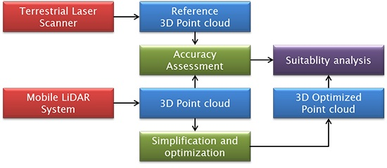
Figure 2 the global pipeline for the geometric accuracy and optimized assessment data aimed at 3D web visualization and dissemination is shown.
3D data acquired by active sensors (TLS and MLS) are processed following a conventional workflow. In the case of TLS, the obtained unstructured point clouds (individual scans) are cleaned, edited and aligned in a common local reference system. The alignment process can be automatically carried out through Iterative Closest Point (ICP) points [
47], by automatic recognition of objects [
48] or using artificial targets [
49]. The 3D point cloud obtained with milimetric resolution can include the intensity levels (I) and/or the color information (RGB). Finally, the aligned point cloud is georeferenced in a global reference system by means of targets of known coordinates. Regarding the MLS, three main types of sensors take part in data acquisition using three independent reference systems. A multi-sensor calibration is mandatory to determine the translational and rotational offsets among the different sensors and bring all the data into the same reference system [
50]. As a result, the unstructured point cloud is already aligned in a global reference system by means of the navigation/positioning sensors with centimetric absolute precision (typically). The 3D point cloud obtained uses to have also a centimetric resolution, including at least the intensity levels of returned pulses or even the color information (RGB).
3.1. Accuracy Assessment Protocol
Since the MLS involves several sensors (e.g., IMU, LiDAR, GNSS, etc.) to acquire a georeferenced 3D point cloud, the aim of this step is to analyze, in the CH field, the quality of the MLS point cloud using a ground truth provided by a TLS. To dismiss the uncertainties associated to the global coordinate geo-referencing, a registration phase with the Iterative Closest Point (ICP) technique is carried out, prior to the MLS point cloud evaluation [
51]. As a result, only those errors affecting the 3D point cloud of the architectural elements are analyzed. Particularly, discrepancies are computed in consonance with Multiscale Model to Model Cloud Comparison (M3C2) [
52], which performs a direct comparison of the 3D point clouds (TLS to MLS), avoiding the preliminary phase of meshing.
In order to prevent possible bias effects affecting the data processing, the normality assumption, i.e., the hypothesis that errors follow a Gaussian distribution, are checked according to graphical methods such as QQ-plot [
53] well-suited for very large samples [
54]. If the samples are not normally distributed, either due to the presence of outliers or because of a different population hypothesis, a robust model based on non-parametric estimation should be employed. In this case, the median (
m) and the median absolute deviation (MAD) are used as robust measures instead of the mean and standard deviation, respectively. The MAD is defined as the median (
m) of the absolute deviations from the data’s median (
mx):
where the
xi values come from the discrepancies (Euclidean distance) between both point clouds (TLS and MLS).
The computation of the discrepancies maps is carried out by Cloud Compare v2.7.0 software [
55], being a point cloud-to-point cloud based on the M3C2 plugin [
52]. The robust statistical estimators are computed by a custom script as well as the in-house statistical software (STAR (Statistics Tests for Analyzing of Residuals)) [
56].
3.2. Point Cloud Optimization
Despite recent technological breakthroughs, it is still common to face some limitations since 3D datasets obtained by active sensors (TLS and MLS) produce complex reality-based 3D point clouds which are generally large. For extensive CH sites, the geometric component hinders the access for analysis purposes through Web visualization, worsen when mobile devices (e.g., tablets or smartphones) are used, due to the vast amount of information. Depending on the device used and the size of the 3D models, a delay might occur that could affect the fluidity of the 3D scene. Moreover, the 3D point cloud acts as mainframe for the extraction of semantic and/or vector information, avoiding the meshing step. The common algorithms used to generate a mesh are time-consuming, since they require human intervention to correct topological errors (e.g., non-manifold edges, loose edges, overlapping faces, self-intersections, etc.) that could be generated, and the holes filling required to rebuild those areas affected by errors and occlusions. Thus, different simplification and optimization strategies would be desirable to be applied to the 3D point clouds, while keeping the relevant information for the subsequent studies and/or operations in the global pipeline of CH conservation and management.
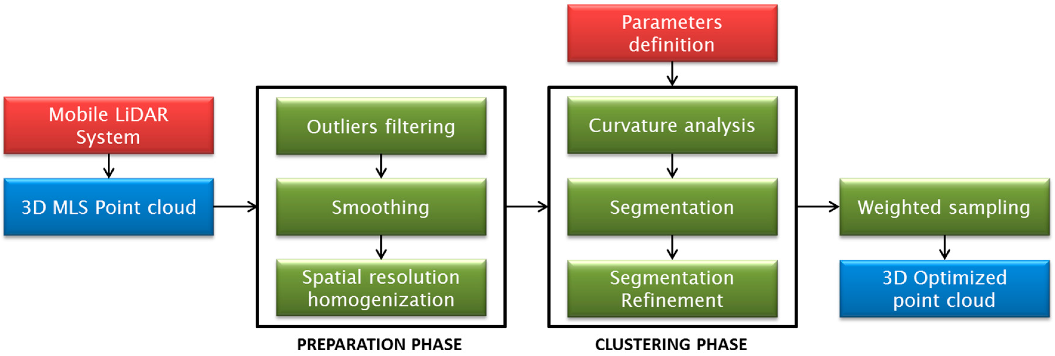
The proposed optimization methodology (
Figure 3) is based on an idealization process and an adaptive sampling according to a confidence interval and local feature curvature. Thus, the more significant are the points, the more 3D points are kept to represent those complex areas of the site. On the contrary, for those parametric and simple geometrical CH elements such as planes, the point cloud is considerably reduced in size.
The point cloud optimization strategy has been developed following three global phases: (i) a preparation phase to setup the raw point cloud acquired from MLS; (ii) a clustering phase based on a curvature segmentation; and (iii) a final weighted sampling phase.
The
preparation phase involves three sub steps in the following order:
An initial outliers filtering of the MLS point cloud based on the absolute deviation (Euclidean distance) of the points from a fitted local plane in a spherical vicinity. The absolute threshold is not set very strictly to avoid false positives. In the case a plane cannot be fitted in the neighborhood, the point is also excluded.
Next, in order to ease the simplification, a local smoothing process by means of a moving least squares [
57] is applied. This operation involves a point displacement regarding the original positions; however, the spherical search volume is chosen in relation to the precision obtained from the accuracy assessment studies (see
Section 3.1) to avoid a precision deterioration of the final optimized point cloud.
Finally, a reduction of high point density areas, due to the MLS acquisition methodology, is applied. For this task, a spatial sampling is carried out. The sampling value determines the final results. Since there are several options for this sampling value, all of them being related to the input point cloud precision, the proposed one is to setup the 95% confidence interval of the error dispersion from the accuracy assessment studies. By this procedure, it is possible to guarantee the optimized final results.
Once the point cloud is ready, the
curvature clustering phase is carried out following the next three sub steps:
Initially, the local curvature is computed in a wide spherical neighborhood to reduce noise effects. The spherical radius for the curvature calculation is defined in relation to the main geometrical elements of the CH site (i.e., a-priori length and height).
Next, the 3D point cloud is segmented according to the computed local curvature and the a-priori approximate knowledge of the main geometrical primitives presented (e.g., planes and radius of cylinders). These coarse values allow defining a discrete number of clusters according to a similar curvature values. The final number of clusters is increased in one, since the highest curvature values are related to non-parametric areas, as the break-lines, borders, corners, abrupt areas, surface discontinuities or geometric and topological errors.
Finally, since the curvature computation and clustering could be affected by local errors, especially in transition areas, a refinement based on connected component analysis is carried out to reclassify them in the more suitable cluster. This analysis is based on an octree representation of the point cloud, so a reference subdivision level has to be set. In order to find connected components, the octree level has to be set slightly higher than the homogenized spatial resolution. Since the spatial resolution was homogenized in the preparation phase, and an octree level has to be fixed, it is possible to relate easily the component’s area by the number of points. For the main features of the CH site, it is possible to define their minimum area. As result, the components inside a cluster that do not verify this minimum area are reallocated to the neighbor cluster in crescent curvature. No points are removed.
Lastly, a weighted sampling is applied to all the points inside a cluster based on the associated feature (e.g., plane, cylinder, etc.) and based on the maximum and minimum curvature values of the cluster. The highest curvature cluster is kept unmodified, since encloses all the conflictive areas. The others cluster thresholds, low and medium curvature, are established according to its geometric elements. For instance, the number of points of a wall could be drastically reduced if points can be assimilated/idealized as a plane. In the cases of other elements as towers, the arc to chord approximation was used. Thus, a final 3D optimized point cloud is obtained, retaining all the geometrical relevant information for subsequent tasks, as vectorization, reverse engineering, finite element (FEM) analysis and information management through HBIM or even for Web visualization.
4. Experimental Results
The case study was the Medieval Wall of Avila. Its construction is the most important example of military architecture of the Spanish Romanesque style as well as an exceptional model of European medieval architecture [
58]. The construction of the city wall is perfectly adapted to the topography. The wall was used not only to defend the town from possible invasions and protect the people from possible pests or epidemics, but also to control the trade of the city with the outside. The southern sectors are shorter as they are built upon a cliff that acts as a natural defense. The western and northern sections grow in height, reaching the tallest and thickest points located in the east section. There are nine gates giving access to the town, of which the most spectacular is “
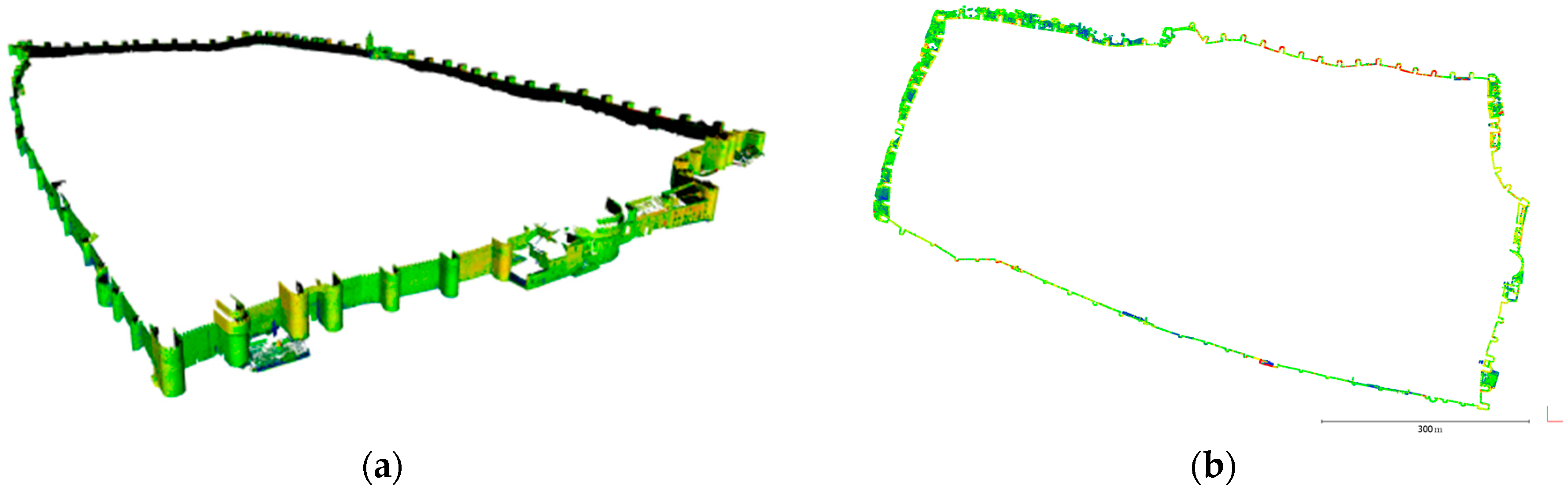
Puerta del Alcázar” (Gate of the Fortress). In 1884, it was declared a National Monument and in 1985, the old city of Ávila and its extramural churches were declared a World Heritage site by UNESCO. Some references state that the building dates back to 1090. Other researchers have argued instead that the wall’s construction most likely continued through into the 12th century. Its large size is a clear example of a challenging CH sites for the recording and documentation processes. Despite its linear nature (
Figure 4), the towers and wall distribution, the gates, and neighbor city buildings add difficulties for acquisition and processing. Since the case study presents a repetitive pattern (i.e., wall–tower–wall) along its whole extension, only a significant part of its extension was evaluated. Thus, the obtained results could be extrapolated to the whole medieval Wall. The main geometric information is shown in
Table 3.
The 3D point cloud of the whole medieval wall coming from the TLS was carried out using the process described in [
59]. The spatial resolution achieved was 15 mm for an average scanning distance of 20 m. The georeferencing of the TLS into a global coordinate system (ETRS89) was done by a GNSS network of 50 control points, using two Leica 1200 GPS, distributed in the towers and the upper part of the wall as well as along its base. The registration errors of the individual TLS scans have been evaluated by a network of control points, analyzing its propagation in a close object. The discrepancies reached up to 5 cm as stated in [
59]. The TLS workload involved 159 h for the 2.5 km perimeter wall.
The 3D point cloud obtained (
Figure 5) by means of MLS of the whole Medieval Wall of Avila was carried out according to the process described in [
60]. The spatial resolution acquired was 60 mm for an average scanning distance of 25 m. The georeferencing of the LiDAR 3D point cloud into a global coordinate system was done by the integrated IMU sensor (Applanix POS LV 520) on the LYNX Mobile Mapper.
MLS and TLS workload, in terms of time consumption and accuracy, is compared in
Table 4.
4.1. Point Cloud Accuracy Assessment
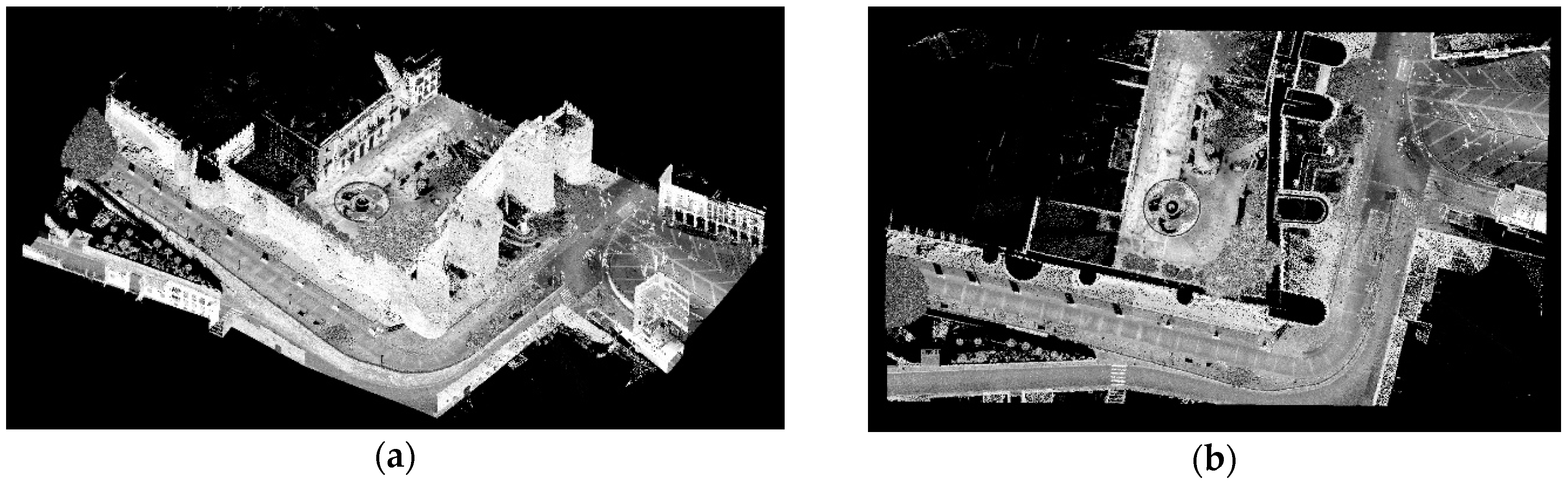
The accuracy assessment was focused in the named “Alcazar” door, one of the highest wall entrances (
Figure 6), and its vicinity, originally annex to the “Alcazar” fortress, where the defensive system was reinforced with a barbican and a ditch.
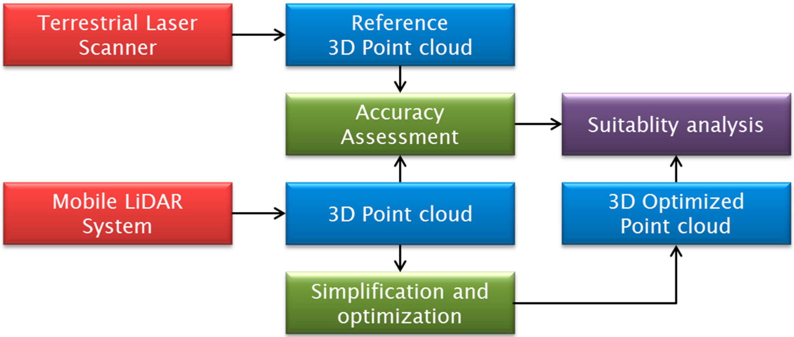
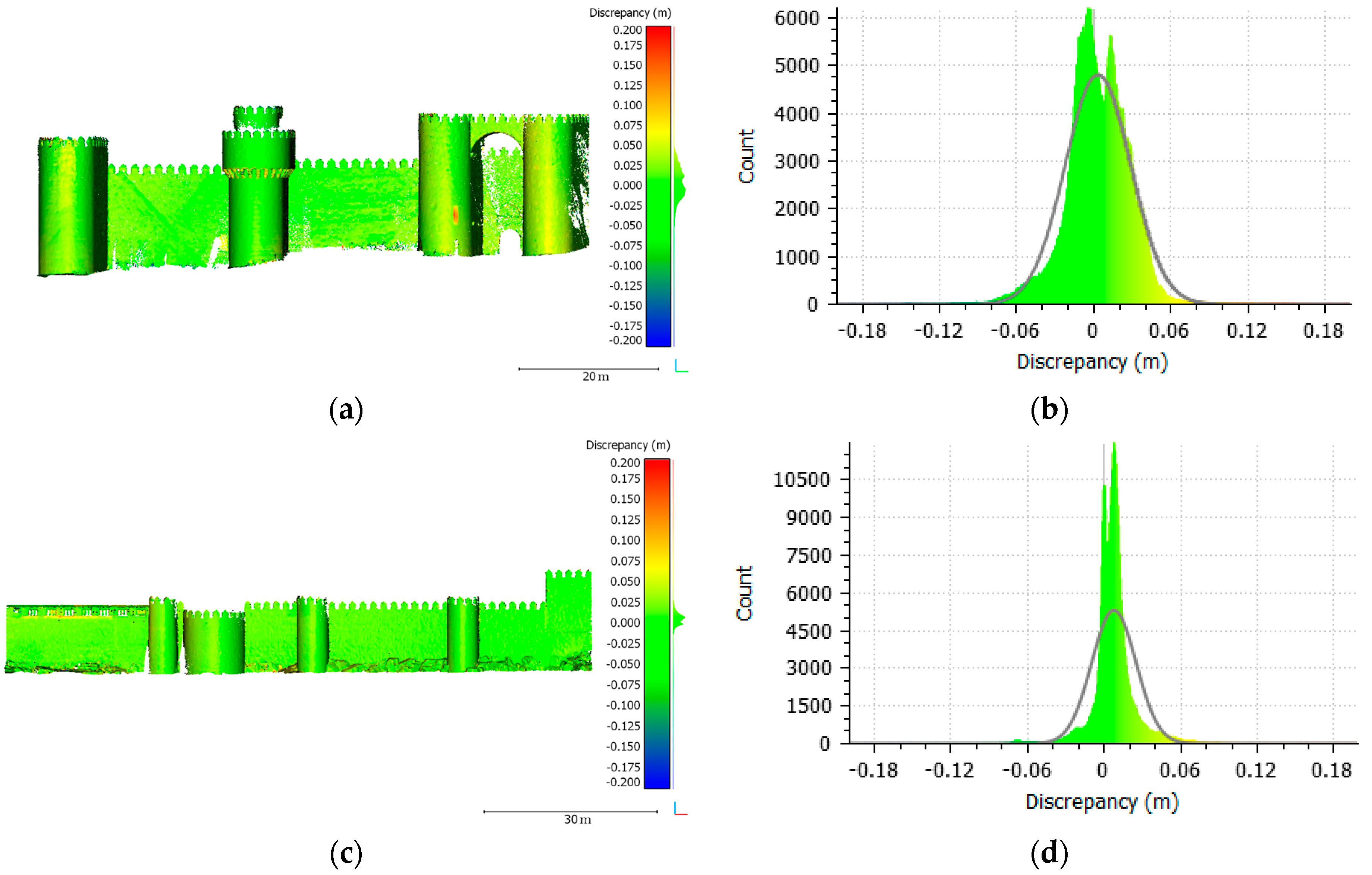
The georeferencing error of the MLS is dependent on three factors: the GNSS system, the trajectory compensation and the calibration method of its sensors. The georeferencing error of the TLS is associated with the two GPS receivers used. Thus, in order to evaluate the accuracy of a MLS point cloud, a registration phase with ICP was carried out. Consequently, a comparison of both 3D point clouds was done (TLS and MLS). After the removal of the non-overlap areas (e.g., parts acquired by the MLS but not by the TLS), the discrepancies map was computed, as shown in
Figure 7, separately for the east walls (
Figure 7a) and the south walls (
Figure 7c), which delimitated the fortress. These discrepancies were computed using the point cloud-to-point cloud comparison, obtained as the result of the signed error between both point clouds.
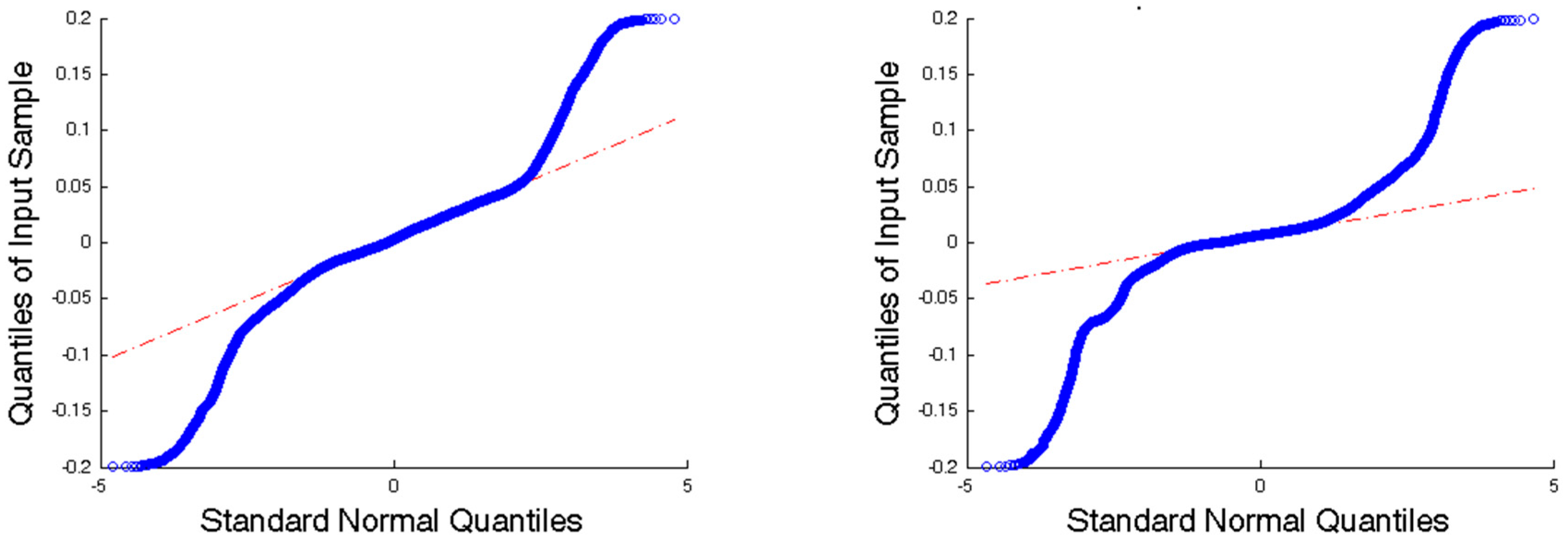
The obtained values were analyzed with a QQ-plot to confirm the non-normality of the sample (
Figure 8). This fact was hinted by the histogram shape (
Figure 7b,d), but since it is directly dependent on the bin size, it cannot be used as decision criterion. Since this sample does not follow a normal distribution (
Figure 8), it is not possible to infer the central tendency and dispersion of the population according to Gaussian statistics parameters such as mean and standard deviation. For that reason, the accuracy assessment was computed based on robust alternatives, using non-parametric assumptions such as the median and the MAD value shown in
Table 5.
In this analysis, the median value is close to zero (2.8 mm in the east wall), as was expected after the application of the ICP registration algorithm. However, a slightly higher value of 6.9 mm is appreciated in the south wall, which points to some registration error, but it is inside the expected range. Moreover, in
Table 5, the dispersion value (MAD) is according to the expected error, confirming the MLS a-priori reference values, especially in the south wall, which has a simple geometry (
Figure 7c). The analysis of the error sample by means of the non-parametric estimator for the quantile, yields that the 95% of the error points are inside the [−0.046 m; 0.047 m] interval. This reference value is used in the optimization phase to carry out the point cloud simplification.
It is worth noting that, despite the symmetrical shape of the sample in the east wall (as shown in the first and third quartile), there is a high difference (up to three times) between the standard deviation and the MAD having as reference the south wall. The conclusions would seem wrong without an adequate statistical parameter selection.
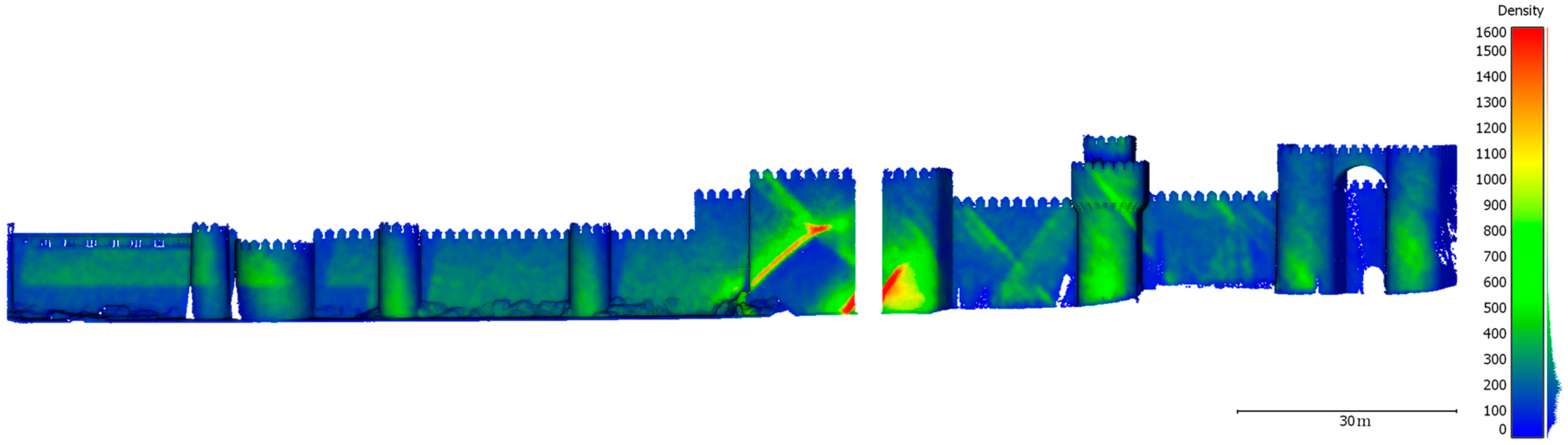
In conclusion, the spatial resolution achieved by the MLS and his distribution is directly related to the sensor–object distance; therefore, there will be areas with higher point density than others (
Figure 9). Moreover, in
Figure 9, some diagonal stripes are shown by cause of inhomogeneity in the acquisition phase due to the oblique laser scanner heads arrangement in the vehicle (
Figure 1). This fact is not a critical issue, but reinforces the necessity of a 3D point cloud data optimization that copes with those redundant areas.
According to an ideal equilateral triangles distribution for a circular neighborhood [
61], the average point density achieved is 58.8 mm, decreasing up to a spatial resolution of 135 mm for the farthest zones (e.g., battements and upper parts of towers). In addition, the occlusion in these zones underestimates the density computation since the point vicinity is incomplete.
4.2. Optimization Analysis
In the Medieval Wall of Avila, two main features are clearly recognized: the planar walls and the cylindrical towers. On the one hand, the walls are considered to have zero curvature, but due to the construction processes and the deterioration of the structures caused by the course of time, the actual conservation state does not keep this property. Therefore, a slight curvature of 0.005 m−1 (200 m radius) can be assumed. Additionally, the individual stones of the wall also contribute to local groups of higher curvature, so this threshold is extended to the annexed towers. On the other hand, in the case of the towers, the diameters of the cylinders range from 4.5 to 10 m. Accordingly, the upper limit for the curvature cluster is set as 0.4 m−1. The rest of the elements (e.g., battlements, arrow slits or natural rocks) are contained in a final cluster of higher local curvature.
The size of these main elements (walls and towers) suggests a wide neighborhood for the computations to balance the curvature precision and noise effects. The minimum height of 10 m and the typical wall width of 20 m favors this large neighborhood. By a selection of a spherical diameter of 2 m for the curvature computation, implicitly, a security buffer of 1 m is kept between the different clusters. Additionally, a minimum area of 1 m2 per cluster is set as threshold for the clustering refinement.
As the final parameter definition, the sampling interval for the homogenization is chosen as 5 cm, which, according to
Section 4.1, is the nearest round value corresponding to the 95% non-parametric confidence interval of the MLS point clouds. In the first step of the
preparation phase, 0.4% of points were excluded as outliers, since they exceeded the point to local plane distance of 20 cm. As result, after the smoothing process and the spatial resolution homogenization, 521,090 points were obtained, which implies a 47.4% reduction of the original input.
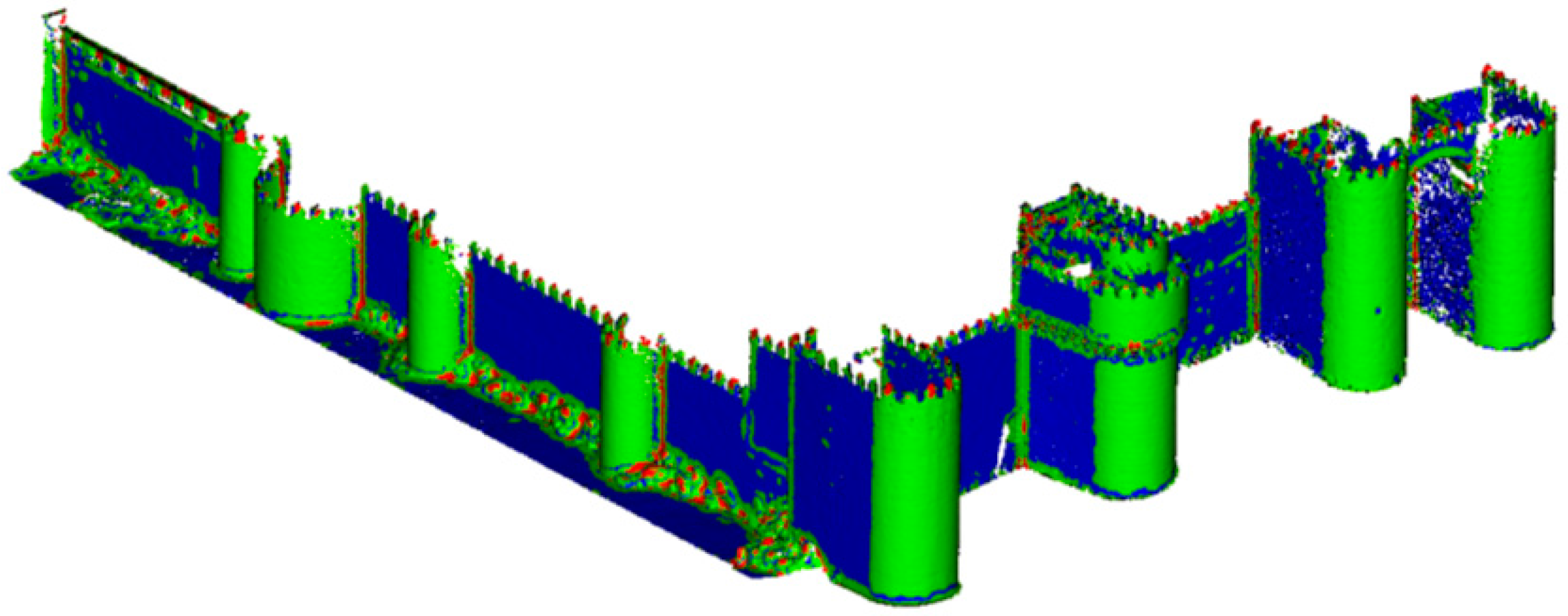
Next, the curvature analysis is carried out for a spherical neighborhood of 1 m of radius, which is segmented according the three pre-established clusters: (i) planar or low curvature (<0.05 m
−1); (ii) cylindrical, mild transitions and medium curvature (0.05–0.40 m
−1); and (iii) the abrupt transitions of high curvature (>0.40 m
−1). The results are outlined in
Figure 10.
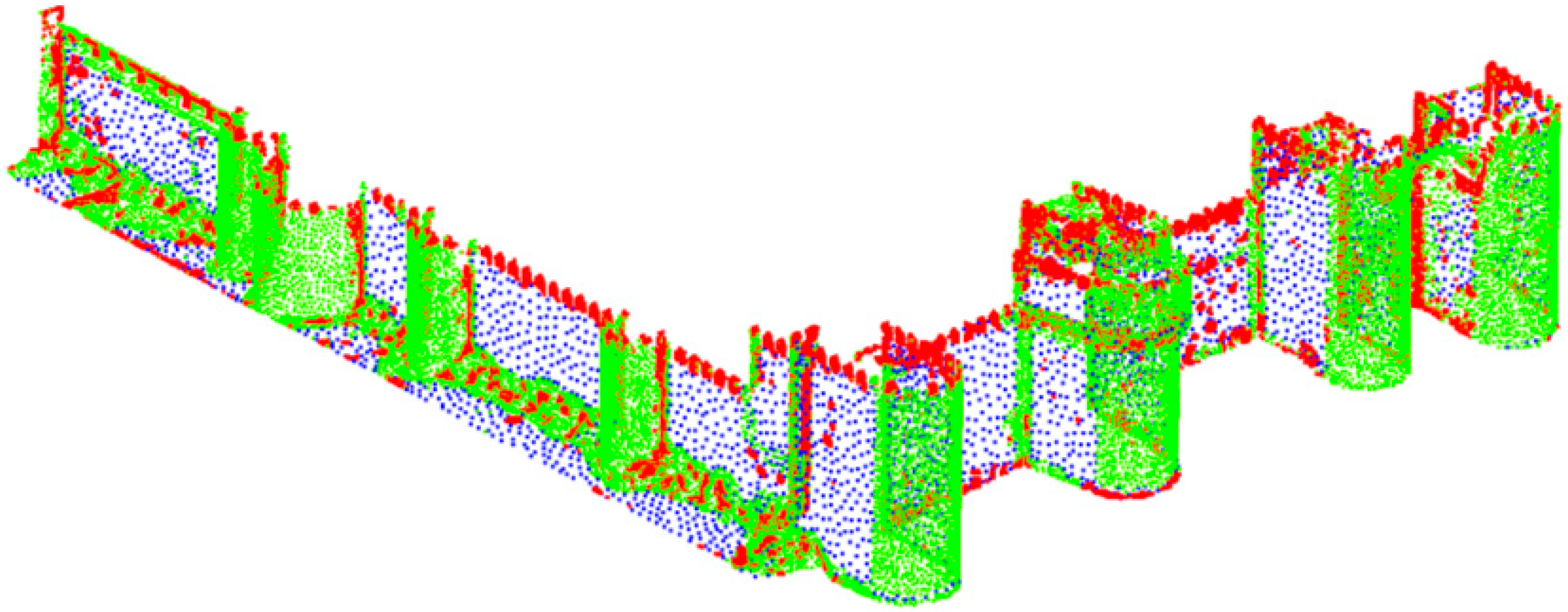
Subsequently, these clusters are refined based on a connected components analysis. The octree level is chosen in relation to a reference spatial sampling of 0.12 m, which corresponds to 160 points per square meter.
Table 6 shows the percentage of reallocated components per cluster and the final classification. For the low curvature cluster, the main planar elements are coded by only 47 components, the rest being small components (about two thousand) located in the transition area of the wall planes, and in the transition to the battlements. Despite the high number of affected components, more than 97% of cluster components, they only represent a small fraction of the classified 3D points in the cluster. Similarly, for the cylindrical, mild transitions and medium curvature cluster, the reallocated components are located in the battlements and in some abrupt rocks distribution inside the curtain walls. In the case of the battlements, this behavior is caused due to their small size in relation to the curvature spherical vicinity used for the computation. However, due to the optimization protocol, they are moved to a cluster with crescent curvature in order to keep a higher spatial density. In the case of natural rocks aggrupation located in the wall, their curvature was lower than the threshold for the high curvature cluster (>0.4 m
−1). As result of the minimum area threshold, they were reallocated in the high curvature cluster since they were heterogeneously disposed in the curtain walls.
Finally, the weighted sampling is applied inside the clusters. For the low curvature, a resolution of 1 m is chosen, since the smooth process and plane-to-curve idealization. In the intermediate cluster, aimed for the towers, an arc to chord assimilation is applied. For a 50 cm chord, the idealization error will cause a sagittal of 13 mm for the worst case, which is inside the acceptable limits. Therefore, a 0.5 m weighted sampling is set. Lastly, the high curvature cluster is kept unmodified. The final point cloud has 58,476 points (
Figure 11), which implies a reduction of 88.8% in relation to the spatially homogenized point cloud (521,090 points), and 94.1% in relation to the raw point cloud.
5. Discussion
The novel use of MLS applied to the 3D surveying of large Cultural Heritage sites is evaluated and compared with the TLS, which is currently the most common technology used for this purpose.
MLS device combines different sensors on a mobile platform that allows obtaining an accurate and georeferenced 3D point cloud. Active sensors together with Inertial and Global Navigation System are synchronized in real time to collect and store data. The active sensor acquires detailed 3D points from a local coordinate system, while the IMU and GNSS systems provide and correct 3D points under a global reference frame. Moreover, some MLS can acquire RGB information captured by photographic or video cameras. Although the MLS spatial resolution depends on the active sensor (laser scanner) integrated on the mobile platform, usually the point clouds acquired by MLS cannot compete with TLS in terms of high resolution. Nevertheless, for large CH sites, the use of MLS could be more suitable, allowing the mapping of large and complex sites in an efficient way (e.g., historical cities or landscapes).
Otherwise, MLS reduces the data acquisition time thanks to the use of a mobile platform, while TLS needs multiple stations (sometimes even hundreds) to cover a large area. There are two main advantages of MLS technology compared to other 3D recording systems: (i) MLS is less expensive than airborne LiDAR systems boarded on airplanes or helicopters; and (ii) MLS can acquire accurate 3D data faster than TLS. On the contrary, its main disadvantage is that sometimes the transit with vans or cars is not possible due to conservation reasons or limitations of space (e.g., narrow streets). In this last case, it is possible to board the MLS on alternative platforms such as quads [
62], backpack [
16] or even autonomous robots [
17].
MLS also reduces the data processing time in comparison with TLS, especially in large and complex CH sites. MLS directly produces a single point cloud, georeferenced with centimetric accuracy due to the IMU and GNSS calibrated sensors, whereas the 3D data captured by TLS have to be aligned in a relative or global reference system.
Finally, the visualization and management of large datasets still represent a bottleneck for both techniques (MLS and TLS). The ongoing development of 3D recording sensors and data capture technologies are advancing more rapidly than the management of large geometrical datasets. MLS and TLS usually produce massive point clouds (millions of points) requiring storage spaces of many GB. To advance this problem, 3D datasets (i.e., point clouds) need to be efficiently optimized and simplified for architectural and structural analysis (e.g., FEM), documentation and management (e.g., HBIM) or outreach purposes (e.g., Web Visualization). As additional benefits of the proposed point cloud optimization, the optimized point cloud will be improved for subsequent 3D modeling tasks based on meshing or reverse engineering procedures, improving the computational time and the resulting geometric definition.
In this paper, our main contribution was based on the use of algorithms and methodologies for the point cloud optimization, without any prior surface reconstruction. There are numerous algorithms to reduce the 3D point cloud in automatic way, but our approach was focused on an adaptive sampling that depends on the geometric features and also keeps the main structures without losing relevant details. The optimal solution was to find a compromise between the resolution acquired, the accuracy and the final size of the file, in order to obtain detailed 3D point clouds that could be stored, managed and visualized with a fluent real-time interaction.
6. Conclusions
This paper deals with a novel use of Mobile LiDAR System for the 3D recording of large Cultural Heritage sites. As part of the suitability assessment of this technology, an accuracy evaluation with a Terrestrial Laser Scanner was carried out. The obtained results, checked in an appropriate study case, allow us to confirm the suitability of Mobile LiDAR System techniques for 3D recording and modeling of large Cultural Heritage sites.
On the one hand, we were focused on time consumption. Comparing both 3D recording techniques, Mobile LiDAR System technology was a clear winner in terms of time used for data acquisition and data processing. Data coming from our study case shows that Mobile LiDAR System took only 1 h to sweep an area of 250,000 m2 while the Terrestrial Laser Scanner took 159 h. This means considerable time saving.
On the other hand, spatial resolution was our concern. Terrestrial Laser Scanner could achieve a point cloud density of 15 mm (average of scanning distance: 20 m) while Mobile LiDAR System density was 60 mm (average of scanning distance: 25 m). In order to evaluate data accuracy of the Mobile LiDAR System, a comparison of both 3D point clouds was done, regarding the georeferencing error. Considering that the represented area involved a few kilometers, the results show that 95% of the MLS points acquired are inside of the tolerance range [−0.046 m; +0.047 m]. Even if Mobile LiDAR System provides a less dense point cloud, it is conclusive that it has enough spatial resolution and quality to provide the reconstruction of the most relevant architectural details in large Cultural Heritage sites.
In any case, due to the huge amount of acquired data, the final point clouds should be necessarily optimized for visualization and management purposes. A novel process for point cloud optimization is introduced to facilitate its handling by scholars from various disciplines. The proposed optimization methodology was based on a detail geometric analysis, allowing classifying the different structures into three main clusters (low, medium and high curvature). Different optimization parameters were used for each cluster according to their curvature, obtaining a reduced point cloud ca. 94.1% less in relation to the entire raw point cloud and guaranteeing an optimal solution for multiple purposes.
The results confirm that Mobile LiDAR System also shows more efficiency in terms of operation flexibility, acquisition and processing time, producing high quality and accurate data. However, shape complexity and surrounding characteristics, such as the environment location or the access restrictions, must be taken into account in further studies to define which is the best approach.
In the worst case, when the geometric complexity of the scene is high, the transit of vehicles is difficult or they are restricted access to the archaeological sites, the novel indoor LiDAR technologies (e.g., the backpack solution, mobile robots or the handheld LiDAR mapping system) could be used as an alternative outdoor solution.
To conclude, it would be interesting to extend our approach integrating different outdoors and indoors mobile techniques for large and complex Cultural Heritage sites.


 ,
, 


