Article

Scalable Bag of Subpaths Kernel for Learning on Hierarchical Image Representations and Multi-Source Remote Sensing Data Classification

University Bretagne-Sud, UMR 6074, IRISA, F-56000 Vannes, France
*
Author to whom correspondence should be addressed.
Remote Sens. 2017, 9(3), 196; https://doi.org/10.3390/rs9030196
Submission received: 31 December 2016 / Revised: 9 February 2017 / Accepted: 15 February 2017 / Published: 24 February 2017

Abstract

:
The geographic object-based image analysis (GEOBIA) framework has gained increasing interest for the last decade. One of its key advantages is the hierarchical representation of an image, where object topological features can be extracted and modeled in the form of structured data. We thus propose to use a structured kernel relying on the concept of bag of subpaths to directly cope with such features. The kernel can be approximated using random Fourier features, allowing it to be applied on a large structure size (the number of objects in the structured data) and large volumes of data (the number of pixels or regions for training). With the so-called scalable bag of subpaths kernel (SBoSK), we also introduce a novel multi-source classification approach performing machine learning directly on a hierarchical image representation built from two images at different resolutions under the GEOBIA framework. Experiments run on an urban classification task show that the proposed approach run on a single image improves the classification overall accuracy in comparison with conventional approaches from 2% to 5% depending on the training set size and that fusing two images allows a supplementary 4% accuracy gain. Additional evaluations on public available large-scale datasets illustrate further the potential of SBoSK, with overall accuracy rates improvement ranging from 1% to 11% depending on the considered setup.

Graphical Abstract

1. Introduction

The geographic object-based image analysis (GEOBIA) framework has gained increasing interest for the last decade, especially when dealing with very high resolution remote sensing images [1]. One of its key advantages is the hierarchical image representation through a tree structure, where objects-of-interest can be revealed at various scales (nodes) and where the topological relationship between objects (e.g., A is part of B, or B consists of A) can be easily modeled (edges). In the classification context, however, most papers in the literature deal with only one scale, as pointed out in [2].
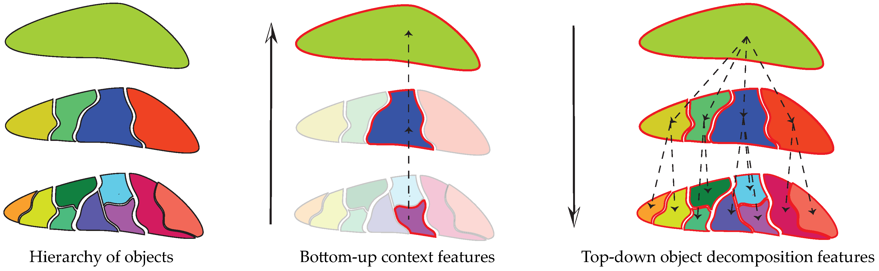
Under the GEOBIA framework, we can extract, depending on the problem at hand, different types of topological features across the scales from a hierarchical representation: bottom-up context features or top-down object decomposition features, as illustrated in Figure 1.
Bottom-up context features (Figure 1, center) model the evolution of a region (leaf of the hierarchical representation) and describe it by its ancestor regions at multiple scales. Such context information helps to disambiguate similar regions during the classification phase [3]. For instance, individual tree species at the bottom scale can be classified into residential area instead of forest zone given surrounding regions being buildings and roads. Integrating such information leads to classification accuracy improvement and produces a spatially smoother classification map [3,4,5].
Top-down object decomposition features (Figure 1, right) model the composition of an object (top of the hierarchical representation) and the topological relationships among its subparts. For instance, a residential area is much easier to identify when knowing it is composed of houses and roads. Including such information can improve the classification rate, especially in high resolution remote sensing imagery cases where the decomposition of objects can be better revealed [6,7].
Although features extracted from the hierarchical representations are considered as discriminative characteristics for classification, dedicated machine learning algorithms still remain largely unexploited for learning directly on these features. In the GEOBIA framework, the most common way to take into account such features is through constructing rules for classifying objects and refining classification results [4,8,9,10]. However, such a knowledge-based subjective rule-set designing strategy is highly reliant on human involvement and interpretation, which makes it difficult to be adapted to new locations and datasets and makes the processing of data in large remote sensing archives practically impossible. Dedicated machine learning methods that are able to fully benefit from the hierarchical representations remain largely underdeveloped. Our previous work in [11] introduced a structured kernel operating on paths (or sequences of nodes) that allows learning from the bottom-up context features, and in [12], we proposed a structured kernel on trees that makes modeling the top-down object decomposition features possible. Despite their superiority for improving the classification accuracy, the major issue of the proposed structured kernels is the computation complexity. This limits the application of these kernels, which are only suitable for small data volume and small structure size.
Meanwhile, data fusion approaches have gained increasing interest recently in the remote sensing community [13]. These techniques aim to integrate information from different sources and to produce fused data with more detailed information. For instance, combining high-resolution imagery and LiDAR data allows better accuracy achievements in an urban area classification task [14]. As the availability of multi-resolution remote sensing data is rapidly increasing, developing methods able to fuse data from multiple sources and multiple resolutions to improve classification accuracy is becoming an important topic in remote sensing [13,15].
In this paper (this paper is an extended version of the conference paper presented at GEOBIA 2016 [16]), we propose a structured kernel based on the concept of the subpath that extracts vertical hierarchical relationships among nodes in the structured data. It can be considered as a kernel operating on paths (or sequences of nodes) that allows learning from the bottom-up context features or a kernel working on trees that models the top-down object decomposition features. The kernel computation is done by explicit mapping of the kernel into a randomized low dimensional feature space using random Fourier features (RFF). The inner product of the transformed feature vector on low dimensional feature space approximates the kernel on structured data. It yields a linear complexity O ( S ) w.r.t. size S (i.e., the number of nodes) of structured data G and a linear complexity O ( n ) w.r.t. number n of training samples. Therefore, the resulting approximation scheme makes the kernel applicable for large-scale real-world problems. We call the kernel scalable bag of subpaths kernel (SBoSK). When referring to the exact computation scheme, we will write BoSK (bag of subpaths kernel).
We also introduce a novel multi-source classification approach operating on a hierarchical image representation built from two images at different resolutions. Both images capture the same geographical area with different sensors and are naturally fused together through the hierarchical representation, where coarser levels are built from a low spatial resolution (LSR) or a medium spatial resolution (MSR) image, while finer levels are generated from a high spatial resolution (HSR) or a very high spatial resolution (VHSR) image. SBoSK is then used to perform machine learning directly on the constructed hierarchical representation.
The paper is organized as follows: a brief review of related works is provided in Section 2. We then describe in Section 3 the structured kernel (BoSK) and its approximated computation using RFF (SBoSK). The multi-source classification approach relying on BoSK/SBoSK is proposed and evaluated on an urban classification task in Section 4. Evaluations on two additional publicly available remote sensing datasets are given in Section 5 before we conclude the paper and provide future research directions.

2. Related Work

The proposed kernel can be applied for learning from both context and object decomposition features and is also introduced to perform the data fusion with a pair of images from different sources and resolutions. Its computation technique enables its use in a large-scale machine learning context. In what follows, we briefly review related works in all of these aspects.

2.1. Context Features

Context features’ modeling is considered as one of the challenges in the GEOBIA framework [1]. Incorporating such features is useful, as it can reveal the surrounding objects at the same scale or model the topological relationships among objects across the scales. For instance, in [8], the authors propose to model topological relations between segmented objects, e.g., roads and moving vehicles, and construct rule-sets for classifying objects and refining classification results. In [9,10], spatial relationships among objects are also used for defining rule-sets. Although designing the knowledge-based rule-set is straightforward to integrate context features into classification, it often requires human involvement and interpretation, which is subjective and hard to adapt to new locations and datasets. Dedicated machine learning techniques that can automatically learn such features need to be developed under the GEOBIA framework.
In the computer vision field, one common way to model the context features is through the conditional random fields technique (CRF) [17]. The CRF defines an energy model containing two terms: the unary potential that measures likelihood of an object belonging to certain classes based on its appearance and the pairwise potentials that model the pairwise relationships between objects. Such technique has been applied for remote sensing datasets [18]. However, most of the remote sensing applications use CRF to enforce smoothness over adjacent regions and increase the classification accuracy (known as the Potts model) [19,20]. This is mainly due to the extremely costly and time-consuming training of a complex model and learning its parameters, as it often requires manual annotation of full scenes.
In the remote sensing community, context features are often taken into account in the feature extraction step, meaning that some spatial features are extracted at the image region level obtained by image segmentation techniques, while the spectral features are extracted at the conventional pixel level. In the end, both spatial and spectral features are combined together and fed into the classifier [21]. Hierarchical representations are often used for extracting context features at multiple scales [3]. Through hierarchy, context features model the evolution of a region and describe it at different levels, one of the most popular example being the attribute profile [22]. Integrating context features leads to classification accuracy improvement in comparison with methods using only spectral information [11]. Since the spatial position is also implicitly taken into account, it often produces a spatially smoother classification map avoiding the “salt and pepper” effect [3,5].

2.2. Object Decomposition Features

Another challenge in the GEOBIA framework is related to the object decomposition features modeling [1]. It is often referred to as the semantic modeling of the object, which represents the composition of an object and the relationships among its subparts. However, techniques consisting of manually modeling such information as developed in the GEOBIA framework require a priori knowledge based on human interpretation to derive proper classification rule-sets [23,24].
In the computer vision community, the spatial pyramid matching (SPM) model [25] is the most common strategy to model the object decomposition features for image classification tasks. The idea is to segment the image into four regions at successive scales (quad-tree representation) and to concatenate all of the region features into a long vector. However, SPM can only capture the absolute object spatial arrangement, as it only allows matching image regions at the same spatial position. Therefore, when applying SPM in remote sensing image classification tasks, such a limitation might cause problems: SPM hardly adapts to images with no predefined location or orientation [6,7,26]. In addition, SPM can only be computed on a quad-tree representation because of its matching strategy, thus preventing its applications on advanced multiscale segmentation techniques generally applied under the GEOBIA framework.

2.3. Data Fusion with Multiple Remote Sensing Images

Data fusion is becoming an important topic in the remote sensing community. Techniques able to fuse data from multiple sources and multiple resolutions have been proven to be effective for improving classification accuracy [15]. As each sensor provides unique spatial details of the observed scene, exploring and combining such information becomes crucial.
Kernel methods have been identified as one of the new research directions for remote sensing data fusion in a recent survey paper [13], as they offer a general framework allowing one to fuse different sources of information in a classification problem. In this framework, each kernel is computed from a different data source, and then, all of the source-specific kernel matrices are combined into a final one that can be later fed into kernel-based classification methods. The combination of several kernels is often done linearly, each kernel being weighted according to its relevance. The weights can be learned using the multiple kernel learning framework [27,28] or simply be determined by cross-validation when the number of kernels is low [21,29]. Such an approach has been applied for combining spectral and spatial information extracted from multi-source [30] and multi-temporal [31] remote sensing images.

2.4. Large-Scale Kernels

Structured kernels have gained increasing attention from various domains as they are able to perform machine learning on structured data (e.g., molecules classification [32], image classification [33]). However, the major issue of such structured kernels is the kernel value computational complexity. This limits the application of structured kernels to a small data volume and a small structure size. Some previous works successfully bring down the kernel computational complexity to be linear, such as [34,35], with the symbolic data type. However, in the case of data equipped with numerical features, it is often reported as quadratic complexity, such as Cui et al. [36] for sequence data, [12] for tree and even worse for the graph kernel, which yields polynomial time [32,33]. As each pair of nodes between two structures has to be at least compared once to compute the overall kernel value, structured kernels on numerical data always yield at least a quadratic complexity. Nevertheless, such high complexity techniques for structured kernels are still in use nowadays [37].
Recently, techniques for kernel value approximation have been well investigated in the context of accelerating the training time in kernel methods [38], e.g., the Nyström method and the random Fourier features technique. The Nyström method approximates the full kernel matrix by a low rank matrix computed with a subset of training examples. Although it has been successfully applied in large-scale machine learning context, it still requires the kernel matrix computation, and this might be time consuming if a large number of subsamples is needed or pairwise kernel value computation is slow, such as in the case of structured kernels. The RFF technique [39,40], however, is a data independent method, which is widely applied due to its efficient computation and approximation quality. The idea is to approximate the kernel by explicitly mapping the data (with basis functions as cosine and sine) into a low dimensional Euclidean space, in which the inner product of the explicit features vector approximate the kernel value. By adopting such a strategy, the empirical study in [41] shows the capability of training on large-scale image recognition problems. In addition, RFF have been applied in order to reduce the computational complexity for the matching kernel that is computed between two sets of local descriptors (e.g., SIFT) extracted from images [42].

3. Kernel Definition and Approximation

3.1. Bag of Subpaths Kernel

Let us define a rooted directed connected acyclic graph G , where nodes n i are defined as a finite set of elements with their numerical features being d-dimensional vectors x n i R d . Depending on the orientation of the edges, we will refer to G as a directed rooted tree T (or tree for short) when it is read away from the root; when read from the leaves towards the root, it can be decomposed as a set of paths P (or sequences of nodes).
In order to capture the vertical hierarchical relationships between the nodes, we decompose either T or P as a set of substructures called subpaths. A subpath is defined as the path connecting a node to one of its descendants (resp. ancestors) in T (resp. P ); the set of subpaths also includes individual nodes. Let us denote a subpath by s p = ( n ( 1 ) , n ( 2 ) , n ( p ) ) , s p G , with ( t ) being the relative position of a node in the subpath, following an ascending order 1 t p , and p being the subpath length. Examples of a tree and a path, together with their sets of subpaths, are shown in Figure 2.
Following the convolution kernel framework [43], kernels can handle structured data by making recursive computations among the parts of the structures. The definition of BoSK between G and G is thus written:
K ( G , G ) = p = 1 P s p G s p G K ( s p , s p )
where the first sum is defined over the different lengths of subpaths, with P being the maximum subpath length extracted from G . The second and third sums allow the computation of the kernel over all pairs of subpaths in G and G (note that only the matching of subpaths of the same length is permitted). The kernel between two subpaths s p and s p is defined as the product of atomic kernels computed on pairs of nodes k ( n ( t ) , n ( t ) ) of the subpaths:
K ( s p , s p ) = t = 1 p k ( n ( t ) , n ( t ) )
The conventional choice of the atomic kernel k ( · ) is the Gaussian kernel as adopted in [11,12,16,33]. In that case, the kernel K ( s p , s p ) can be written as:
K ( s p , s p ) = t = 1 p exp ( γ | | x n ( t ) x n ( t ) | | 2 ) = exp ( γ | | x s p x s p | | 2 ) = ϕ ( x s p ) , ϕ ( x s p ) H
where the x s p R p d is the numerical feature of subpath s p , i.e., x s p = [ x n ( 1 ) T , x n ( 2 ) T , , x n ( p ) T ] T , being the concatenation of the features of the nodes. Following the definition of a kernel function, one can write K ( s p , s p ) in the inner product form in a Hilbert space H as ϕ ( x s p ) , ϕ ( x s p ) H , where ϕ ( · ) is the mapping function for the Gaussian kernel [44].

3.2. Ensuring Scalability Using Random Fourier Features

By using the explicit mapping function for the Gaussian kernel, BoSK can be rewritten as follows:
K ( G , G ) = p = 1 P s p G s p G ϕ ( x s p ) , ϕ ( x s p ) H = p = 1 P s p G ϕ ( x s p ) , s p G ϕ ( x s p ) H
The explicit mapping function ϕ ( · ) hence brings down the quadratic computational complexity of K ( G , G ) to a simple inner product computation with a linear complexity, as the double sum operation changes to a simple sum computed independently for each subpath.
The explicit mapping function ϕ ( · ) definition is then crucial for bringing down the complexity for structured kernel, but it is unknown. Approximations have been well investigated in the context of accelerating the training of kernel machines [38], especially in the context of large-scale learning methods. Here, we consider random Fourier features (RFF) [39,40]: the idea is to approximate the kernel by explicitly mapping the data to a low dimensional Euclidean space, where the inner product of the mapping function z ( · ) approximates the kernel value:
k ( x , x ) = ϕ ( x ) , ϕ ( x ) H z ( x ) T z ( x )
The approximation function z ( · ) [45] for the Gaussian kernel can be written as:
z ( x ) = 2 D cos ( ω 1 x ) sin ( ω 1 x ) cos ( ω D 2 x ) sin ( ω D 2 x ) , ω i i i d N ( 0 , 2 γ )
where D is the dimension of the RFF vector, and the weight vector ω i is drawn from a Gaussian distribution of mean zero and variance 2 γ , γ being the bandwidth parameter of the Gaussian kernel.
We can then write:
K ( G , G ) = τ ( s ) T τ ( s )
where the set of vectors encoded into the feature space for each subpath s p is aggregated inside a single vector τ ( s ) = [ s 1 G z ( x s 1 ) T , , s P G z ( x s P ) T ] T .

3.3. Kernel Normalization

A well-known issue of the structured kernels is that their value highly depends on the size of the structure. This comes from the fact that the overall kernel value relies on summing up all of the kernel values on substructures: the more substructures one can extract, the larger the kernel value is. In the literature, this problem can be mitigated using the kernel normalization strategy [46]:
K * ( G , G ) = K ( G , G ) K ( G , G ) K ( G , G )
We instead propose to adopt a L 2 normalization strategy dedicated to structured kernel using RFF, as it is commonly used as a preprocessing step in the computer vision community before applying the linear kernel [47,48]. To do so, we perform L 2 normalization on the RFF vector for each subpath length before concatenating the normalized vectors together:
τ ( s ) = 1 P s 1 G z ( x s 1 ) T s 1 G z ( x s 1 ) 2 , , s P G z ( x s P ) T s P G z ( x s P ) 2 T
Note that the inner product τ ( s ) T τ ( s ) is a valid kernel as it is equivalent to a sum of kernels computed on each length p then divided by P 2 . In our case, the L 2 normalization strategy has several advantages: (i) the overall kernel value is in ( 0 , 1 ] with the kernel K ( G , G ) = 1 ; (ii) the kernel value of each length p contributes equally to the overall kernel value; (iii) the normalization strategy maintains the vector form of the set of subpaths, which is suitable for large-scale classification tasks based on linear machine learning algorithms.
Further, we propose to limit the maximum considered subpath lengths P in Equation (9) instead of taking it to be the maximum length. This leads to a smaller vector size to be fed into machine learning algorithms and further reduces the computational time as smaller patterns need to be considered.

3.4. Complexity

The proposed approximation, SBoSK, yields a linear complexity of O ( n S d D ) , while the exact computation maintains a quadratic complexity of O ( n 2 S d ) . Figure 3 illustrates BoSK computed on a pair of trees T , T and its scalable SBoSK extension.
The advantage of the RFF embedding can be easily derived from here: (i) the proposed algorithm computes RFF embedding in O ( S d D ) , which is linear w.r.t. the structure size S, thus allowing the use of the proposed structured kernel in the real-world application of a large structure size; (ii) the embedded vector can feed a linear machine for training, which yields a linear dependence w.r.t. the size of training samples of O ( n ) , instead of a non-linear kernel machine that needs to compute a complete kernel matrix that requires a quadratic complexity of O ( n 2 ) .

4. Image Classification with Multi-Source Images

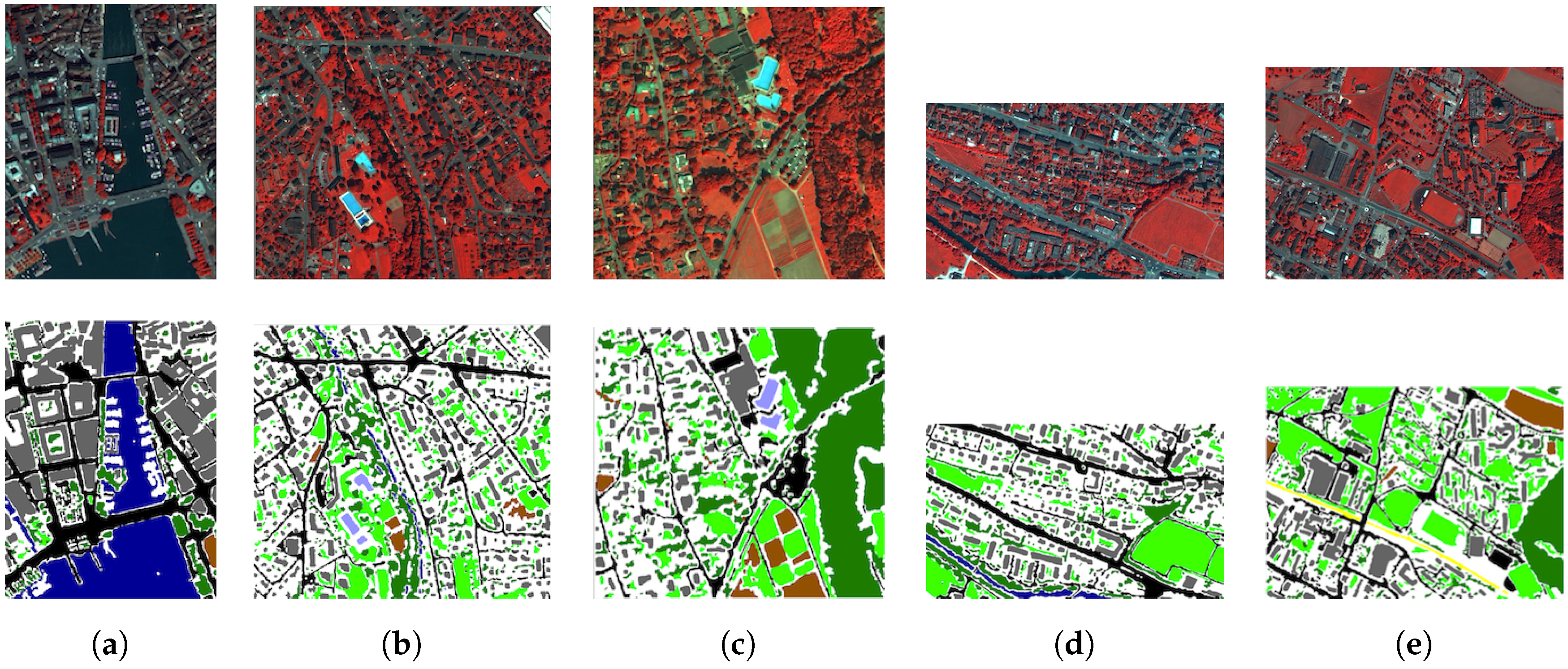
We focus on urban land-use classification in the south of Strasbourg city, France. We consider eight thematic classes of urban patterns described in Table 1 and in Figure 4c (ground truth image). Two images are considered, both capturing the same geographical area with different sources:
  • an MSR image, captured by a Spot-4 sensor, containing 326 × 135 pixels at a 20-m spatial resolution, described by four spectral bands: green, red, NIR, MIR (Figure 4a).
  • a VHSR image, captured by a Pleiades satellite, containing 13,040 × 5400 pixels at a 0.5-m spatial resolution (obtained with pan-sharpening technique), described by four spectral bands: red, green, blue, NIR (Figure 4b).
More details about the images can be found in [49].
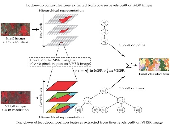
We fuse the two different resolution images into a single hierarchical representation through two separate steps: (i) use the MSR image to construct the coarser levels of the hierarchy where bottom-up context features can be computed on the one side; (ii) use the VHSR image to generate the finer levels of the tree, where top-down object decomposition features are extracted on the other side. The overall process is illustrated in Figure 5.
Firstly, we initialize the segmentation at the pixel level on the MSR image and construct iteratively the coarser levels. Let n 1 be a data instance to be classified. Within the MSR image, it corresponds to a pixel n 1 l and can be featured as a path P = { n 1 l , , n P l } that models the evolution of the pixel n 1 l through the hierarchy. Each node n i l is described by a d-dimensional feature x n i l that encodes the region characteristics, e.g., spectral information, size, shape, etc.
Secondly, we use the VHSR image to provide the fine details of the observed scene for each data instance n 1 . Indeed, one pixel of the MSR image n 1 l always corresponds to a 40 × 40 pixels square region of the VHSR image n 1 h . To do so, we initialize the top level of the multiscale segmentation to be the square regions, then construct the finer levels. Through the hierarchy, the data instance n 1 can be modeled as a tree T rooted in n 1 h , which encodes object decomposition and the topological relationships among its subparts. The characteristics of region n i h are also described by a d-dimensional feature x n i h .
In the end, each data instance n 1 can be represented by an ascending path P from the MSR image and a descending tree T generated from the VHSR image. Such a hierarchical representation allows one to benefit from the bottom-up context features on the coarser levels built from the MSR image, and of the top-down object decomposition features on the finer levels built from the VHSR image.
To generate the hierarchical image representation, we can rely on any multiscale segmentation algorithm. Here, we use HSeg [50], whose parameters have been empirically fixed as follows:
  • On the MSR image, we generate, from the bottom (leaves) level of single pixels, seven additional levels of multiscale segmentation by increasing the region dissimilarity criteria α = [ 2 2 , 2 1 , , 2 4 ] . We observe that with such parameters, the number of segmented regions is roughly decreasing by a factor of two between each level.
  • On the VHSR image, we generate, from the top (root) level of each square region of size 40 × 40 pixels (i.e., equivalent to a single pixel in Strasbourg Spot-4 dataset), four additional levels of multiscale segmentation by decreasing the region dissimilarity criteria α = [ 2 4 , 2 3 , 2 2 , 2 1 ] . Using such parameters, we observe that the number of segmented regions is roughly increasing by a factor of two between each level.
Each region in the hierarchical representation is described by an eight-dimensional feature vector x , which includes the region average of the four original multi-spectral bands, soil brightness index (BI) and NDVI, as well as two Haralick texture measurements computed with the gray level co-occurrence matrix, namely homogeneity and standard deviation. These features are considered as standard ones in the urban analysis context [51].
To perform image classification from a hierarchical representation, we propose to combine structured kernels computed on two types of structured data: SBoSK on paths allows learning from the bottom-up context features at coarse levels on the MSR image, while SBoSK on trees on the VHSR image makes the modeling of the object decomposition features possible. Both kernels exploit complementary information from the hierarchical representation, thus combined together through vector concatenation at the end as:
K ( n 1 , n 1 ) = ρ × K ( P , P ) + ( 1 ρ ) × K ( T , T ) = ρ × τ ( s P ) T τ ( s P ) + ( 1 ρ ) × τ ( s T ) T τ ( s T ) = ρ 1 ρ × τ ( s P ) T , 1 ρ × τ ( s T ) T T ρ 1 ρ × τ ( s P ) T , 1 ρ × τ ( s T ) T
where K ( P , P ) is BoSK (Equation (1)) on paths, K ( T , T ) is BoSK on trees, τ ( s P ) and τ ( s T ) are the RFF embedding of P and T , respectively, according to Equation (9), with a parameter ρ [ 0 , 1 ] that controls the importance ratio between the two kernels. The evaluation of these different kernels is provided in Section 4.2, Section 4.3 and Section 4.4, respectively.
We consider a one-against-one SVM classifier (using the Python implementation of LibSVM [52]) with the Gaussian kernel as the atomic kernel. All free parameters are determined by five-fold cross-validation, which include: the bandwidth γ of Gaussian kernel and the SVM regularization parameter C over potential values, the weight ρ [ 0 , 1 ] between the two structured kernels and the maximum considered subpath length P { 1 , 2 , } . The RFF dimension D is chosen empirically as a trade off between computational complexity and the classification accuracy (and will be further analyzed in Section 4.1).

4.1. Random Fourier Features Analysis

In this section, we compare, in terms of classification accuracy and computation time, BoSK as introduced in [11,12] with the SBoSK proposed here.
We firstly analyze the impact of the number of RFF dimensions in terms of accuracy. To do so, we conduct the experiments on the MSR image considering SBoSK on paths and on the VHSR image relying on SBoSK on trees. We compare BoSK and SBoSK with D = { 2 1 , 2 2 , , 2 13 } . For both experiments, we use 400 training samples per class and the rest for testing and report the results computed over 10 repetitions. As we can observe in Figure 6, when the RFF dimension increases, the accuracy increases until it converges to the accuracy obtained with the exact computation scheme. However, such a classification accuracy convergence rate is problem dependent, and the number of RFF dimensions needed to be used is commonly set empirically [39].
Secondly, we analyze the impact of RFF dimensions in terms of computation time. To do so, we follow the previous setting and use differing training samples per class n = { 50 , 100 , , 1600 } (except when n = 1600 , we use all 1434 available samples for collective housing blocks). As we can see in Figure 7, the computation time increases linearly w.r.t. n for SBoSK, while for its exact computation, it increases quadratically. This indicates the efficiency of the proposed RFF approximation in the context of large-scale machine learning. In addition, we can also observe for SBoSK that the computation time increases linearly w.r.t. dimension D, while the accuracy shown in Figure 6 improves only slightly when D is large. Therefore, one might have to compromise on the quality of approximation and time consumption. Henceforth, in this section, we empirically fix the RFF dimension to be D = 4096 as a trade off between the approximation quality and the complexity.
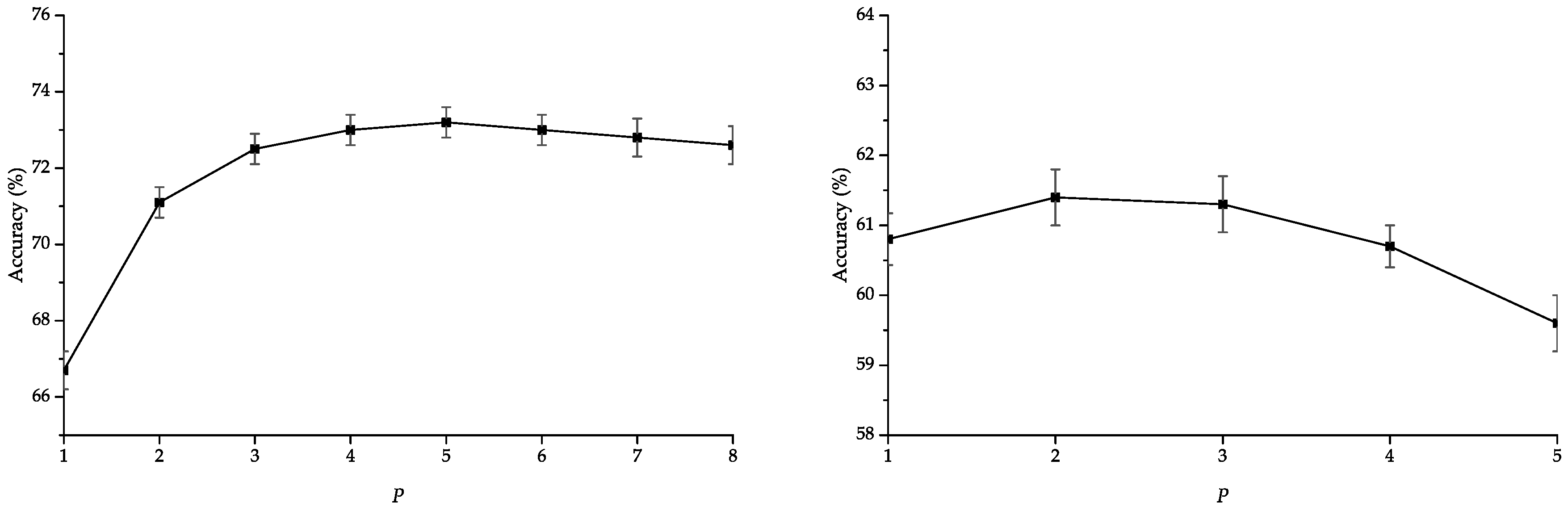
In addition, we analyze the impact of maximum considered subpath length P using our proposed L 2 normalization strategy for SBoSK in Section 3.3. Figure 8 shows that the accuracies improve when considering subpath with different lengths compared to using only nodes i.e., P = 1 . However, the accuracies might decrease when adding the features extracted from longer subpath patterns, thus calling for penalization of longer subpath patterns. Besides, we propose to set a maximum subpath length for SBoSK, leading to a smaller vector size to be fed into machine learning algorithms, which can further reduce the computational time as smaller patterns are being considered.

4.2. Bottom-Up Context Features

In this section, we evaluate SBoSK taking into account bottom-up context features extracted from hierarchical representation built on the Strasbourg MSR image. Each pixel in the image is the data instance to be classified and is represented as a path that can be handled with SBoSK.
For comparison purposes, we consider the Gaussian kernel on the pixel level (without any context/spatial information) as the baseline and compare our work with several well-known techniques for spatial/spectral remote sensing image classification. The spatial-spectral kernel [21] has been introduced to take into account the pixel spectral value and spatial information through accessing the nesting region. We thus implement the spatial-spectral kernel based on the multiscale segmentation commonly used in this paper and select the best level (determined by a cross-validation strategy) to extract spatial information. The attribute profile [22] is considered as one of the most powerful techniques to describe image content through context features. The spatial information is extracted from hierarchical representations (min-tree and max-tree) using multiple thresholds according to different region attributes, e.g., area of the region, standard deviation of spectral information inside the region. We use full multi-spectral bands with automatic level selection for the area attribute and the standard deviation attribute, as detailed in [53]. The stacked vector was adopted in [3,5,54] and relies on features extracted from hierarchical representation. We use a Gaussian kernel with the stacked vector that concatenates all nodes from ascending paths generated from our multiscale segmentation. The comparison is done by randomly choosing n = [ 50 , 100 , 200 , 400 ] samples for training and the rest for testing. All reported results are computed over 10 repetitions for each run.
The classification accuracies with different methods are shown in Table 2. We also give the per-class accuracies using n = 400 training samples in Figure 9.
When compared to the Gaussian kernel on the pixel level using only spectral information, SBoSK taking into account bottom-up context features can significantly improve the classification accuracies. We observe about 20 % accuracy improvement for different training sample sizes. Per-class accuracies indicate that this improvement concentrates on all classes, except two, water surface and forest areas, for which classification accuracies remain similar, since context features extracted from ancestor regions through hierarchy are mostly homogeneous.
SBoSK achieves about 5 % improvement over the spatial-spectral kernel and attribute profile for various training sample sizes. For these two state-of-the-art methods considering spatial information, the results actually depend on the selected scales. However, for the spatial-spectral kernel relying on a single scale, it is hard to define such a single scale that fits all objects, as it is commonly known in the GEOBIA framework that objects are often revealed through various scales. Therefore, for certain classes, e.g., urban vegetation, it might yield good results with the selected scale. However, it is difficult to generalize for all classes. On the other hand, the attribute profile requires setting the thresholds for different attributes in order to achieve good classification results. However, as indicated in [55], generic strategies for filter parameters’ selection for different attributes are still lacking.
Comparing to the Gaussian kernel with stacked vector, SBoSK achieves about 8 % classification accuracy improvement for various training sample sizes. Since both kernels rely on the same paths, it demonstrates the superiority of SBoSK for taking into account context features extracted from a hierarchical representation. In fact, the Gaussian kernel with the stacked vector is actually a special case of BoSK with the subpath length equal to the maximum (illustrated in our previous study [11]). However, structured kernels built only on the largest substructures are usually not robust [11]. Indeed, larger substructures are often penalized when building the structured kernels [35]. In our experiment, this superiority is presented in the per-class accuracies for all except two homogeneous classes: water surface and forest areas.

4.3. Top-Down Object Decomposition Features

In this section, we evaluate SBoSK taking into account top-down object decomposition features extracted from hierarchical representation built on the Strasbourg VHSR image. Each square region of 40 × 40 pixels in the image is the data instance to be classified and is represented as a tree that can be handled with SBoSK.
For comparison, we consider the SPM model [25], which is well known in the computer vision community for taking into account the spatial relationship between a region and its subregions. The SPM relies on a quad-tree image segmentation, which splits each image region iteratively into four square regions. In this representation, the pyramid Level 0 (root) corresponds to the whole image, and Level 2 (L2) segments image regions into 16 square regions. For a fair comparison, we build SBoSK on the same spatial pyramid representation. However, let us recall that SBoSK can rely on an arbitrary hierarchical representation. We thus also report the results computed on a hierarchical representation generated using the Hseg segmentation tool. The comparison is done by randomly choosing n = [ 50 , 100 , 200 , 400 ] samples for training and the rest for testing. All reported results are computed over 10 repetitions of each run.
The classification accuracies obtained with different methods are shown in Table 3. We also provide per-class accuracies using n = 400 training samples in Figure 10.
When compared to the Gaussian kernel computed on root regions, SBoSK consistently improves the classification results for various numbers of training samples. Furthermore, the improvements increase when more training samples are added, i.e., from 2.1 % OA/ 1.2 % AA improvement with 50 training samples per class to 4.9 % OA/ 3.9 % AA with 400 training samples per class. Analysis of the per-class accuracies leads to observing that industrial blocks and individual housing blocks, two semantically similar classes, benefit from the highest improvement among all classes. This is due to SBoSK ability to consider top-down object decomposition features and spatial relationship among its subparts.
As far as the SPM model is concerned, we can see that it performs poorly with various training samples: the results drop down 3 % to 4 % compared to the kernel computed on the root region. Although SPM has been proven to be effective in the computer vision domain due to its capacity of coping with subregions and spatial arrangement between subregions, its one-to-one region matching strategy with the exact spatial location constraint seems overstrict for remote sensing image classification. Indeed, it lacks image orientation invariance, which is required when dealing with nadir observation. To illustrate, in both individual and collective housing block classes, the orientation and absolute location of objects, such as the houses in each image ( 40 × 40 pixels region), are not discriminated, and thus, this is not helpful for improving classification accuracy. However, such irrelevant features cannot be excluded in the SPM model due to its matching strategy. Therefore, two images with similar content, but with different spatial locations and orientations might be classified into two different classes.
We also compare SBoSK applied on different hierarchical representations. Results show that SBoSK on Hseg segmentation leads to better results than when computed on spatial pyramid representation. From per-class accuracies, we can see that the industrial blocks, individual housing blocks and collective housing blocks, i.e., semantically similar classes, are better classified. This can be easily explained by the shapes of the segmented regions: while spatial pyramid representation splits the image into four square regions independently of the actual image content, the Hseg segmentation provides a more accurate segmentation, since similar regions are naturally merged together into larger regions iteratively through the hierarchy.

4.4. Combining Context and Object Decomposition Features

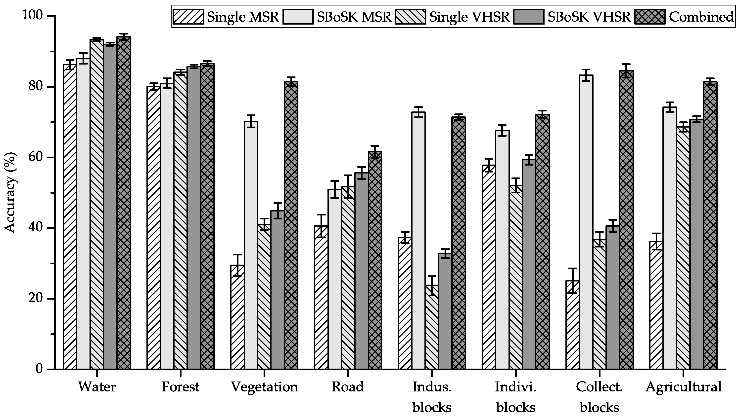
In this section, we evaluate our proposed multi-source images classification technique and represent each data instance by both an ascending path P in the MSR image and a descending tree T in the VHSR image.
For comparison purpose, the following scenarios are considered: (i) Scenario 1: Gaussian kernel at single level on the MSR image vs. SBoSK taking into account the bottom-up context features at multiple levels on the MSR image; (ii) Scenario 2: Gaussian kernel at single level on the VHSR image vs. SBoSK taking into account the top-down object decomposition features at multiple levels on the VHSR image; (iii) Scenario 3: combining both the context and object decomposition features extracted from a hierarchical representation using both MSR and VHSR images.
The classification accuracies achieved with the different methods are shown in Table 4 using various numbers of training samples n = [ 50 , 100 , 200 , 400 ] . We also show the per-class accuracies for eight different classes using n = 400 training samples in Figure 11.
The classification results show that combining bottom-up and top-down topological features lead to a significant improvement. Indeed, we observe, for various training sample sizes, more than 4 % improvement over SBoSK on a single MSR image and more than 10 % improvement over SBoSK on a single VHSR image. From an analysis of per-class accuracies achieved with SBoSK, we can see that some classes (urban vegetation, industrial blocks, individual and collective housing blocks and agricultural zones) yield higher accuracies on the MSR image, while some other classes (water surfaces, forest areas, roads) obtained better accuracies on the VHSR image. Nevertheless, combining both kernels allows benefiting from the advantages of the two complementary features, thus yielding the best accuracies for all classes. Indeed, we can state that the prediction achieves a spatial regularization for the large regions (e.g., industrial and individual housing blocks) thanks to the context features, while providing precision for the small structures (such as road networks) thanks to the detailed object decomposition features.
When compared with the Gaussian kernel computed on a single image at a single level, combining both SBoSK built on two different image sources achieves 13 % OA improvement when using n = 50 and 20 % OA improvement when using n = 400 . This demonstrates the superiority of our proposed multi-source classification method that is able exploiting topological features across multiple scales within the GEOBIA framework.

5. Evaluations on Large-Scale Datasets

In this section, we evaluate SBoSK on two large-scale publicly available datasets. The term large-scale refers to a large number of training samples for the Zurich summer dataset (more than 10,000 data instances for training and 1,000,000 for testing) or a large structure size for the UC Merced dataset (more than 300 nodes for each structured data). These numbers are considered as large scale in the context of classification using structured kernel, where evaluated datasets are normally made of thousands of data instances with a few dozens of nodes each [32]. For these two datasets, due to the quadratic complexity, BoSK cannot be computed, so only SBoSK is applied. The RFF dimension has been empirically set at 4096.

5.1. Zurich Summer Dataset

The “Zurich Summer v1.0” dataset [18] is a collection of 20 images, taken from a QuickBird acquisition of the city of Zurich with pansharpened resolution of about 0.62 cm. The images are composed of four channels (NIR, R, G, B), with an average image size of ca. 1000 × 1150 pixels. Examples of the dataset (Images 16 to 20 with associated ground truth in eight different annotated urban classes) are shown in Figure 12.
We evaluate SBoSK taking into account bottom-up context features extracted from a hierarchical representation built on the dataset. Each pixel in the image is considered as a data instance to be classified and is represented as a path that can be handled with SBoSK.
For each image, we generate from the bottom level of each single pixel six additional levels of hierarchical segmentation with the Hseg segmentation tool using the region dissimilarity criteria α = [ 2 0 , 2 1 , , 2 5 ] . Each region in the hierarchical representation is described by a 24-dimensional feature vector: the min, max, average and standard deviation values of the pixels included in the region for each spectral band and two derived channels (NDVI and NDWI). As such, we are using the same feature set as in [56].
To allow a fair comparison with the state-of-the-art, we follow the experimental setup provided in [56]: using Images 1 to 15 for training (with a selection stratified of 0.1 % available training samples per class, which corresponds to 12,263 pixels chosen from all training images) and Images 16 to 20 for evaluation. The final classification results is computed over 10 repetitions for random dataset splits into training and evaluation sets.
The OA and AA results are shown in Table 5 for individual Images 16 to 20, reporting results averaged over 10 repetitions. We can see that the kernel computed at the single pixel using only spectral information yields the worst results compared to the methods taking into account context information. Comparing to the state-of-the-art method using conditional random fields [56], building kernels on a hierarchical representation (i.e., spatial-spectral, attribute profile, stacked vector) can provide a better result. More interestingly, SBoSK further improves the results achieved with the stacked vector relying on the same paths, leading to the overall best results. Classification maps obtained with SBoSK are given in Figure 13. SBoSK produces spatially smooth classification maps, with most of the compact regions being correctly predicted.

5.2. UC Merced Dataset

The “UC Merced land-use” (UC Merced) dataset [26] consists of 2100 images with 256 × 256 pixels and a 0.3 -m resolution. Those images are equally distributed in 21 land use classes, with examples from each class shown in Figure 14.
We evaluate SBoSK taking into account top-down objects arrangement features extracted from hierarchical representations built on the dataset. Each image of 256 × 256 pixels is considered as a data instance to be classified and is represented as a tree that can be handled with SBoSK.
In our experiment, we use two different hierarchical image representations: for the spatial pyramid representation, we define five levels in the pyramid that segments the image into { 1 , 4 , 16 , 64 , 256 } regions. The bottom level L4 corresponds to image regions of size 16 × 16 pixels. For the hierarchical representation generated with Hseg segmentation, we define five levels of hierarchy, by empirically setting the dissimilarity criteria α = [ 2 5 , 2 4 , 2 3 , 2 2 ] . Such parameters yield a similar number of segmented regions at the bottom level between both hierarchical representations, thus easing comparison between the different methods. The region feature is generated from dense SIFT descriptors with a fixed window size of 8 × 8 pixels and a step size of one pixel. It is characterized with a quantized histogram of size (also known as codebook size) K = { 50 , 100 , 300 , 500 , 1000 } with the K-means algorithm and max-pooling strategy, as used in [6]. Finally, we use the Gaussian kernel computed on the square-rooted histogram [57] for each region of SPM model and SBoSK.
All reported results are conducted consistently with previous evaluation procedures on this dataset [6,26]: we randomly split the dataset to allow five-fold cross-validation and return averaged results over 10 repetitions for each randomly split dataset.
The results are shown in Table 6 with different codebook sizes K = { 50 , 100 , 300 , 500 , 1000 } . We can see that SBoSK outperforms other methods for different codebook sizes, and the improvement is especially significant when the codebook size is small.
We can see that the SPM model improves the Gaussian kernel on the root region when using two levels of pyramid (L2). However, the results drop down dramatically when four levels of pyramid (L4) are considered. This is due to the overstrict one-to-one region matching strategy adopted in SPM model (as previously discussed). On the other side, SBoSK can further improve the results when adding more pyramid representation levels from L2 to L4. This demonstrates the superiority of the proposed matching strategy relying on bags of subpaths.
The pyramid of spatial relatons [6] is a recently proposed method tackling the issues raised when applying the SPM kernel on geographic images. However, we can see that SBoSK yields better results with various codebook sizes K, and the gap is significant especially when K is small. Indeed, the pyramid of spatial relatons performs similarly as SPM kernel for 100 bins, i.e., ca. 4 % less than SBoSK using L2 and 8 % less than SBoSK using L4.
Finally, when comparing SBoSK with different underlying hierarchical representations, we can notice that Hseg segmentation improves the results when the codebook size K is small. This indicates that classification results can benefit from a better hierarchical representation when region features are less discriminant. Since the object decomposition features are better revealed with Hseg segmentation, we claim that such topological features are especially useful when the region appearance feature is not discriminant enough.

6. Conclusions

In this paper, we propose a structured kernel to cope with bottom-up context features and top-down object decomposition features extracted from a hierarchical representation under the GEOBIA framework, called SBoSK. Its computation is done using random Fourier features to approximate the kernel value, which brings down the complexity from quadratic to linear w.r.t. structure size O ( S ) and training data size O ( n ) . Relying on SBoSK, we also introduce a novel multi-source classification approach using two images with different spatial resolutions. This paper demonstrates the need for integrating dedicated machine learning algorithms to take into consideration the topological relationships between objects under the GEOBIA framework. Indeed, evaluations performed on a urban classification task and on large-scale datasets show that SBoSK allows significant accuracy improvements w.r.t. state-of-the-art techniques. Furthermore, the multi-source approach further benefits from the hierarchical kernel, as it allows enhanced performances when compared to classification at a single scale.
In the future, we plan to investigate several directions. We first plan to learn the discriminative subpath substructures and to weight them accordingly. We also would like to focus on other dimension reduction techniques in order to further accelerate the training time.

Acknowledgments

The authors acknowledge the support of the French Agence Nationale de la Recherche (ANR) under Reference ANR-13-JS02-0005-01 (Asterix project) and the support of Région Bretagne and Conseil Général du Morbihan (ARIA doctoral project). The authors would also like to thank A. Puissant from LIVE UMR CNRS 7362 (University of Strasbourg) for providing the Strasbourg dataset (Spot-4 and Pleiades images with associated ground truth).

Author Contributions

All authors have made major contributions: Yanwei Cui conceived, designed and performed the experiments; Laetitia Chapel, Sebastien Lefevre analysed and interpreted the results; all authors have been involved in the writing of the manuscript.

Conflicts of Interest

The authors declare no conflict of interest.

References

  1. Blaschke, T.; Hay, G.J.; Kelly, M.; Lang, S.; Hofmann, P.; Addink, E.; Feitosa, R.Q.; van der Meer, F.; van der Werff, H.; van Coillie, F.; et al. Geographic Object-Based Image Analysis—Towards a new paradigm. ISPRS J. Photogramm. Remote Sens. 2014, 87, 180–191. [Google Scholar] [CrossRef] [PubMed]
  2. Blaschke, T. Object based image analysis for remote sensing. ISPRS J. Photogramm. Remote Sens. 2010, 65, 2–16. [Google Scholar] [CrossRef]
  3. Bruzzone, L.; Carlin, L. A Multilevel Context-Based System for Classification of Very High Spatial Resolution Images. IEEE Trans. Geosci. Remote Sens 2006, 44, 2587–2600. [Google Scholar] [CrossRef]
  4. Shackelford, A.K.; Davis, C.H. A combined fuzzy pixel-based and object-based approach for classification of high-resolution multispectral data over urban areas. IEEE Trans. Geosci. Remote Sens. 2003, 41, 2354–2363. [Google Scholar] [CrossRef]
  5. Lefèvre, S.; Chapel, L.; Merciol, F. Hyperspectral image classification from multiscale description with constrained connectivity and metric learning. In Proceedings of the 6th International Workshop on Hyperspectral Image and Signal Processing: Evolution in Remote Sensing, Lausanne, Switzerland, 24–27 June 2014.
  6. Chen, S.; Tian, Y. Pyramid of spatial relatons for scene-level land use classification. IEEE Trans. Geosci. Remote Sens. 2015, 53, 1947–1957. [Google Scholar] [CrossRef]
  7. Zhao, B.; Zhong, Y.; Zhang, L. A spectral-structural bag-of-features scene classifier for very high spatial resolution remote sensing imagery. ISPRS J. Photogramm. Remote Sens. 2016, 116, 73–85. [Google Scholar] [CrossRef]
  8. Liu, Y.; Guo, Q.; Kelly, M. A framework of region-based spatial relations for non-overlapping features and its application in object based image analysis. ISPRS J. Photogramm. Remote Sens. 2008, 63, 461–475. [Google Scholar] [CrossRef]
  9. Qiao, C.; Wang, J.; Shang, J.; Daneshfar, B. Spatial relationship-assisted classification from high-resolution remote sensing imagery. Int. J. Digit. Earth 2015, 8, 710–726. [Google Scholar] [CrossRef]
  10. Aksoy, S.; Cinbis, R.G. Image mining using directional spatial constraints. IEEE Geosci. Remote Sens. Lett. 2010, 7, 33–37. [Google Scholar] [CrossRef] [Green Version]
  11. Cui, Y.; Chapel, L.; Lefèvre, S. Combining multiscale features for classification of hyperspectral images: A sequence based kernel approach. In Proceedings of the 8th IEEE International Workshop on Hyperspectral Image and Signal Processing: Evolution in Remote Sensing, Los Angeles, LA, USA, 21–24 August 2016.
  12. Cui, Y.; Chapel, L.; Lefèvre, S. A subpath kernel for learning hierarchical image representations. In Proceedings of the International Workshop on Graph-Based Representations in Pattern Recognition, Beijing, China, 13–15 May 2015; pp. 34–43.
  13. Gomez-Chova, L.; Tuia, D.; Moser, G.; Camps-Valls, G. Multimodal classification of remote sensing images: A review and future directions. Proc. IEEE 2015, 103, 1560–1584. [Google Scholar] [CrossRef]
  14. Chen, Y.; Su, W.; Li, J.; Sun, Z. Hierarchical object oriented classification using very high resolution imagery and LIDAR data over urban areas. Adv. Space Res. 2009, 43, 1101–1110. [Google Scholar] [CrossRef]
  15. Zhang, J. Multi-source remote sensing data fusion: Status and trends. Int. J. Image Data Fusion 2010, 1, 5–24. [Google Scholar] [CrossRef]
  16. Cui, Y.; Lefèvre, S.; Chapel, L.; Puissant, A. Combining Multiple Resolutions into Hierarchical Representations for kernel-based Image Classification. In Proceedings of the International Conference on Geographic Object-Based Image Analysis, Enschede, The Netherlands, 14–16 September 2016.
  17. Nowozin, S.; Lampert, C.H. Structured learning and prediction in computer vision. Found. Trends Comput. Graph. Vis. 2011, 6, 185–365. [Google Scholar] [CrossRef]
  18. Volpi, M.; Ferrari, V. Semantic segmentation of urban scenes by learning local class interactions. In Proceedings of the IEEE Conference on Computer Vision and Pattern Recognition Workshops, Boston, MA, USA, 7–12 June 2015; pp. 1–9.
  19. Schindler, K. An overview and comparison of smooth labeling methods for land-cover classification. IEEE Trans. Geosci. Remote Sens. 2012, 50, 4534–4545. [Google Scholar] [CrossRef]
  20. Damodaran, B.B.; Nidamanuri, R.R.; Tarabalka, Y. Dynamic ensemble selection approach for hyperspectral image classification with joint spectral and spatial information. IEEE J. Sel. Top. Appl. Earth Obs. Remote Sens. 2015, 8, 2405–2417. [Google Scholar] [CrossRef]
  21. Fauvel, M.; Chanussot, J.; Benediktsson, J.A. A spatial–spectral kernel-based approach for the classification of remote-sensing images. Pattern Recognit. 2012, 45, 381–392. [Google Scholar] [CrossRef]
  22. Dalla Mura, M.; Benediktsson, J.A.; Waske, B.; Bruzzone, L. Extended profiles with morphological attribute filters for the analysis of hyperspectral data. Int. J. Remote Sens. 2010, 31, 5975–5991. [Google Scholar] [CrossRef]
  23. Eisank, C.; Drăguţ, L.; Götz, J.; Blaschke, T. Developing a semantic model of glacial landforms for object-based terrain classification—The example of glacial cirques. In Proceedings of the Geographic Object-Based Image Analysis (GEOBIA), Ghent, Belgium, 29 June–2 July 2010; pp. 1682–1777.
  24. Argyridis, A.; Argialas, D.P. A fuzzy spatial reasoner for multi-scale GEOBIA ontologies. Photogramm. Eng. Remote Sens. 2015, 81, 491–498. [Google Scholar] [CrossRef]
  25. Yang, J.; Yu, K.; Gong, Y.; Huang, T. Linear spatial pyramid matching using sparse coding for image classification. In Proceedings of the IEEE Conference on Computer Vision and Pattern Recognition, Miami, FL, USA, 20–26 June 2009; pp. 1794–1801.
  26. Yang, Y.; Newsam, S. Bag-of-visual-words and spatial extensions for land-use classification. In Proceedings of the 18th SIGSPATIAL International Conference on Advances in Geographic Information Systems, San Jose, CA, USA, 2–5 November 2010; pp. 270–279.
  27. Gönen, M.; Alpaydın, E. Multiple kernel learning algorithms. J. Mach. Learn. Res. 2011, 12, 2211–2268. [Google Scholar]
  28. Anees, A.; Aryal, J.; O’Reilly, M.M.; Gale, T.J.; Wardlaw, T. A robust multi-kernel change detection framework for detecting leaf beetle defoliation using Landsat 7 ETM+ data. ISPRS J. Photogramm. Remote Sens. 2016, 122, 167–178. [Google Scholar] [CrossRef]
  29. Camps-Valls, G.; Gomez-Chova, L.; Muñoz-Marí, J.; Vila-Francés, J.; Calpe-Maravilla, J. Composite kernels for hyperspectral image classification. IEEE Geosci. Remote Sens. Lett. 2006, 3, 93–97. [Google Scholar] [CrossRef]
  30. Tuia, D.; Ratle, F.; Pozdnoukhov, A.; Camps-Valls, G. Multisource composite kernels for urban-image classification. IEEE Geosci. Remote Sens. Lett. 2010, 7, 88–92. [Google Scholar] [CrossRef]
  31. Camps-Valls, G.; Gómez-Chova, L.; Muñoz-Marí, J.; Rojo-Álvarez, J.L.; Martínez-Ramón, M. Kernel-based framework for multitemporal and multisource remote sensing data classification and change detection. IEEE Trans. Geosci. Remote Sens. 2008, 46, 1822–1835. [Google Scholar] [CrossRef] [Green Version]
  32. Mahé, P.; Vert, J.P. Graph kernels based on tree patterns for molecules. Mach. Learn. 2009, 75, 3–35. [Google Scholar] [CrossRef]
  33. Harchaoui, Z.; Bach, F. Image classification with segmentation graph kernels. In Proceedings of the IEEE Conference on Computer Vision and Pattern Recognition, Rio de Janeiro, Brazil, 14–21 October 2007; pp. 1–8.
  34. Vishwanathan, S.; Smola, A.J. Fast kernels for string and tree matching. In Kernel Methods in Computational Biology; MIT Press: Cambridge, MA, USA, 2004; pp. 113–130. [Google Scholar]
  35. Kimura, D.; Kashima, H. Fast Computation of Subpath Kernel for Trees. In Proceedings of the 29th International Conference on Machine Learning, Edinburgh, UK, 26 June–1 July 2012; pp. 393–400.
  36. Cuturi, M. Fast global alignment kernels. In Proceedings of the 28th International Conference on Machine Learning, Bellevue, WA, USA, 28 June–2 July 2011; pp. 929–936.
  37. Garro, V.; Giachetti, A. Scale space graph representation and kernel matching for non rigid and textured 3D shape retrieval. IEEE Trans. Pattern Anal. Mach. Intell. 2016, 38, 1258–1271. [Google Scholar] [CrossRef] [PubMed]
  38. Yang, T.; Li, Y.F.; Mahdavi, M.; Jin, R.; Zhou, Z.H. Nyström method vs random fourier features: A theoretical and empirical comparison. In Proceedings of the Advances in Neural Information Processing Systems, Lake Tahoe, NV, USA, 3–6 December 2012; pp. 476–484.
  39. Rahimi, A.; Recht, B. Random features for large-scale kernel machines. In Proceedings of the Advances in Neural Information Processing Systems, Vancouver, BC, Canada, 3–6 December 2007; pp. 1177–1184.
  40. Rahimi, A.; Recht, B. Weighted sums of random kitchen sinks: Replacing minimization with randomization in learning. In Proceedings of the Advances in Neural Information Processing Systems, Vancouver, BC, Canada, 7–10 December 2009; pp. 1313–1320.
  41. Lu, Z.; May, A.; Liu, K.; Garakani, A.B.; Guo, D.; Bellet, A.; Fan, L.; Collins, M.; Kingsbury, B.; Picheny, M.; et al. How to scale up kernel methods to be as good as deep neural nets. arXiv 2014, 14, 1–11. [Google Scholar]
  42. Bo, L.; Sminchisescu, C. Efficient match kernel between sets of features for visual recognition. In Proceedings of the Advances in Neural Information Processing Systems, Vancouver, BC, Canada, 7–10 December 2009; pp. 135–143.
  43. Haussler, D. Convolution Kernels on Discrete Structures; Technical Report; University of California: Santa Cruz, CA, USA, 1999. [Google Scholar]
  44. Shawe-Taylor, J.; Cristianini, N. Kernel Methods for Pattern Analysis; Cambridge University Press: Cambridge, UK, 2004. [Google Scholar]
  45. Sutherland, D.J.; Schneider, J. On the error of random Fourier features. arXiv 2015, 15, 1–11. [Google Scholar]
  46. Collins, M.; Duffy, N. Convolution kernels for natural language. In Proceedings of the Advances in Neural Information Processing Systems, Vancouver, BC, Canada, 3–8 December 2001; pp. 625–632.
  47. Perronnin, F.; Sánchez, J.; Mensink, T. Improving the fisher kernel for large-scale image classification. In Proceedings of the European Conference on Computer Vision, Heraklion, Greece, 5–11 September 2010; pp. 143–156.
  48. Tolias, G.; Avrithis, Y.; Jégou, H. To aggregate or not to aggregate: Selective match kernels for image search. In Proceedings of the IEEE International Conference on Computer Vision, Sydney, Australia, 1–8 December 2013; pp. 1401–1408.
  49. Kurtz, C.; Passat, N.; Gancarski, P.; Puissant, A. Extraction of complex patterns from multiresolution remote sensing images: A hierarchical top-down methodology. Pattern Recognit. 2012, 45, 685–706. [Google Scholar] [CrossRef]
  50. Tilton, J.C. Image segmentation by region growing and spectral clustering with a natural convergence criterion. In Proceedings of the IEEE International Geoscience and Remote Sensing Symposium, Seattle, WA, USA, 6–10 July 1998; pp. 1766–1768.
  51. Forestier, G.; Puissant, A.; Wemmert, C.; Gançarski, P. Knowledge-based region labeling for remote sensing image interpretation. Comput. Environ. Urban Syst. 2012, 36, 470–480. [Google Scholar] [CrossRef]
  52. Chang, C.C.; Lin, C.J. LIBSVM: A library for support vector machines. ACM Trans. Intell. Syst. Technol. 2011, 2, 27. [Google Scholar] [CrossRef]
  53. Ghamisi, P.; Benediktsson, J.A.; Cavallaro, G.; Plaza, A. Automatic framework for spectral–spatial classification based on supervised feature extraction and morphological attribute profiles. IEEE J. Sel. Top. Appl. Earth Obs. Remote Sens. 2014, 7, 2147–2160. [Google Scholar] [CrossRef]
  54. Huo, L.Z.; Tang, P.; Zhang, Z.; Tuia, D. Semisupervised Classification of Remote Sensing Images with Hierarchical Spatial Similarity. IEEE Geosci. Remote Sens. Lett. 2015, 12, 150–154. [Google Scholar]
  55. Ghamisi, P.; Dalla Mura, M.; Benediktsson, J.A. A survey on spectral–spatial classification techniques based on attribute profiles. IEEE Trans. Geosci. Remote Sens. 2015, 53, 2335–2353. [Google Scholar] [CrossRef]
  56. Tuia, D.; Volpi, M.; Moser, G. Getting pixels and regions to agree with conditional random fields. In Proceedings of the IEEE International Geoscience and Remote Sensing Symposium, Beijing, China, 10–15 July 2016; pp. 3290–3293.
  57. Perronnin, F.; Sénchez, J.; Xerox, Y.L. Large-scale image categorization with explicit data embedding. In Proceedings of the IEEE Conference on Computer Vision and Pattern Recognition, San Francisco, CA, USA, 13–18 June 2010; pp. 2297–2304.
Figure 1. An illustration of hierarchy of objects (left); where we can extract bottom-up context features (middle); and top-down object decomposition features (right).
Remotesensing 09 00196 g001
Figure 2. Examples of structured data that can be extracted from hierarchical image representations (a path P models the bottom-up context features; a tree T models the top-down object decomposition features) and their subpaths. (a) A tree T and all of its subpaths s p ; (b) a path P and all of its subpaths s p .
Remotesensing 09 00196 g002
Figure 3. Illustration of a pair of trees T and T (a) with their subpaths s p , s p (b); the computation of BoSK (c) (according to Equation (1)) and scalable bag of subpaths kernel (SBoSK) (d) (according to Equations (7) and (9)). BoSK requires the computation of pairwise kernel value for all training samples, yielding a quadratic complexity w.r.t. training sample size, while SBoSK only needs the computation of the RFF embedded vector τ ( s ) for each structure, yielding a linear complexity w.r.t. training sample size. (a) A pair of trees T (left) and T (right); (b) subpaths for T , T ; (c) BoSK; (d) SBoSK.
Remotesensing 09 00196 g003
Figure 4. Urban scene taken over South of Strasbourg, France. From left to right: false color image of Spot-4 (a) (© CNES2012) with a 20-m resolution; false color image of Pleiades (b) (© CNES 2012, distribution Airbus DS/Spot Image) with a 50-cm resolution; and the associated ground truth (c) (© LIVEUMR7362, adapted from OCSOLCIGAL2012) with eight thematic classes. (a) Spot-4 image; (b) Pleiades image; (c) ground truth image.
Remotesensing 09 00196 g004
Figure 5. Illustration of the hierarchical image representation for two different resolution images. The data instance n 1 to be classified corresponds a pixel of the MSR image n 1 l and a square region on the VHSR image n 1 h .
Remotesensing 09 00196 g005
Figure 6. Overall accuracy (OA) comparison of BoSK and SBoSK with different dimensions D (log scale), computed on the MSR image considering a kernel on paths (left) and on the VHSR image considering a kernel on trees (right). Reported results are computed over 10 repetitions with 400 training samples per class.
Remotesensing 09 00196 g006
Figure 7. Computation time comparison of BoSK and SBoSK with D = { 2048 , 4096 , 8192 } w.r.t. different number of training samples n per class, computed on the MSR image considering a kernel on paths (left) and on the VHSR image considering a kernel on trees (right).
Remotesensing 09 00196 g007
Figure 8. Overall accuracy (OA) w.r.t. different maximum subpath lengths P. SBoSK is computed on the MSR image considering a kernel on paths (left) and on the VHSR image considering a kernel on trees (right) with D = 4096 .
Remotesensing 09 00196 g008
Figure 9. Per-class accuracies using bottom-up context features on the Strasbourg MSR image.
Remotesensing 09 00196 g009
Figure 10. Per-class accuracies using top-down object decomposition features on the Strasbourg VHSR image.
Remotesensing 09 00196 g010
Figure 11. Per-class accuracies for multi-source classification using the Strasbourg MSR and VHSR images.
Remotesensing 09 00196 g011
Figure 12. Examples of Images 16 to 20 (top row) in the Zurich summer dataset, and the associated ground truth (bottom row) with eight different annotated urban classes: roads , buildings , trees , grass , bare soil , water , railways and swimming pools . (a) Image 16; (b) Image 17; (c) Image 18; (d) Image 19; (e) Image 20.
Remotesensing 09 00196 g012
Figure 13. Classification maps of Images 16 to 20 of the Zurich summer dataset using SBoSK.
Remotesensing 09 00196 g013
Figure 14. Examples of the 21 land use classes contained in the UC Merced dataset.
Remotesensing 09 00196 g014
Table 1. List of classes, their color and number of pixels on the MSR image.
ClassColorNb of Pixels
Water surfaces (water)Blue 1653
Forest areas (forest)Dark green 9315
Urban vegetation (vegetation)Light green 1835
Road (road)Grey 3498
Industrial blocks (indus. blocks)Pink 8906
Individual housing blocks (indiv. blocks)Dark orange 9579
Collective housing blocks (collect. blocks)Light orange 1434
Agricultural zones (agricultural)Yellow 7790
Total 44,010
Table 2. Mean (and standard deviation) of overall accuracies (OA) and average accuracies (AA) computed over 10 repetitions for the Strasbourg MSR image with different training data sizes n. The best results (with a statistical significance less than 0.01% against others considering the Wilcoxon signed-rank test for matched samples) are boldfaced.
n PixelSpatial-SpectralAttribute ProfileStacked VectorSBoSK
50OA45.3 (2.3)53.2 (1.0)51.9 (2.1)49.8 (1.8)57.8 (1.3)
AA43.9 (1.0)53.7 (1.4)51.7 (1.4)48.4 (1.1)57.9 (0.8)
100OA47.9 (1.3)57.7 (0.9)57.1 (1.4)54.3 (1.4)63.3 (0.7)
AA46.2 (0.5)59.2 (0.7)57.3 (0.7)52.9 (1.0)64.0 (0.7)
200OA51.4 (0.8)63.1 (0.9)61.7 (0.5)59.0 (0.5)68.4 (0.7)
AA48.1 (0.4)64.6 (0.6)62.2 (0.2)57.5 (0.6)69.7 (0.5)
400OA52.2 (0.4)67.3 (0.8)65.0 (0.5)62.7 (0.6)73.0 (0.4)
AA49.1 (0.2)68.5 (0.5)66.3 (0.4)62.6 (0.4)74.8 (0.4)
Table 3. Mean (and standard deviation) of overall accuracies (OA) and average accuracies (AA) computed over 10 repetitions for the Strasbourg VHSR image with different training data sizes n. The best results (with a statistical significance less than 0.01% against others considering the Wilcoxon signed-rank test for matched samples) are boldfaced, and numbers with * indicate that no statistically-significant conclusions can be drawn when compared with the best results.
n RootSPM (L2)SBoSK (L2)SBoSK (Hseg)
50OA52.2 (0.9)48.3 (1.8)53.2 (1.2)54.3 (0.9)
AA51.2 (0.7)46.9 (1.4)51.7 (0.4)52.4 (1.2)
100OA54.2 (0.6)50.5 (1.3)56.0 (1.1) *56.5 (1.4)
AA53.6 (0.4)49.3 (0.7)54.5 (0.7) *54.9 (1.1)
200OA55.7 (0.6)52.4 (0.8)57.7 (0.7)59.2 (0.9)
AA55.1 (0.3)51.3 (0.3)56.5 (0.5)57.8 (0.9)
400OA56.5 (0.5)54.7 (0.5)59.9 (0.7)61.4 (0.3)
AA56.4 (0.2)53.7 (0.3)59.0 (0.6)60.3 (0.3)
Table 4. Mean (and standard deviation) of overall accuracies (OA) and average accuracies (AA) computed over 10 repetitions for the Strasbourg MSR and VHSR images with different training data sizes n. The best results (with a statistical significance less than 0.01% against others considering the Wilcoxon signed-rank test for matched samples) are boldfaced.
n Single MSRSBoSK MSRSingle VHSRSBoSK VHSRCombined
50OA45.3 (2.3)57.8 (1.3)52.2 (0.9)54.3 (0.9)65.3 (0.6)
AA43.9 (1.0)57.9 (0.8)51.2 (0.7)52.4 (1.2)64.3 (0.8)
100OA47.9 (1.3)63.3 (0.7)54.2 (0.6)56.5 (1.4)69.8 (0.7)
AA46.2 (0.5)64.0 (0.7)53.6 (0.4)54.9 (1.1)69.8 (0.8)
200OA51.4 (0.8)68.4 (0.7)55.7 (0.6)59.2 (0.9)73.9 (0.5)
AA48.1 (0.4)69.7 (0.5)55.1 (0.3)57.8 (0.9)74.8 (0.3)
400OA52.2 (0.4)73.0 (0.4)56.5 (0.5)61.4 (0.3)77.3 (0.3)
AA49.1 (0.2)74.8 (0.4)56.4 (0.2)60.3 (0.3)79.1 (0.4)
Table 5. Mean (and standard deviation) of overall accuracies (OA) and average accuracies (AA) computed over 10 repetitions for the Zurich summer dataset Images 16 to 20. The best results (with a statistical significance less than 0.01% against others considering the Wilcoxon signed-rank test for matched samples) are boldfaced, and numbers with * indicate that no statistically-significant conclusions can be drawn when compared with the best results.
Image PixelCRF [56]Spatial-SpectralAttribute ProfileStacked VectorSBoSK
16OA71.8 (0.8)82.881.6 (0.9)78.5 (0.6)83.4 (0.6) *83.9 (0.5)
AA63.7 (2.1)-62.6 (1.1)62.3 (0.8)68.3 (1.1)70.8 (0.4)
17OA75.1 (0.7)82.680.3 (0.6)80.7 (0.9)82.1 (0.6)83.2 (0.6)
AA61.2 (3.6)-66.3 (1.8)60.8 (1.9)65.3 (1.6)67.7 (3.3)
18OA81.1 (0.8)73.085.1 (0.7)83.1 (1.4)85.7 (0.6)87.5 (0.3)
AA74.0 (3.1)-78.6 (1.2)74.5 (3.5)78.6 (1.6)82.4 (0.6)
19OA69.7 (0.7)67.572.1 (1.8)78.4 (1.2)74.8 (0.6)76.0 (0.6)
AA71.5 (0.9)-77.2 (1.5)80.4 (2.3)76.2 (2.9)79.6 (1.4) *
20OA76.9 (1.1)80.283.6 (0.9)81.2 (1.2)82.2 (1.2)84.0 (1.3)
AA74.2 (1.2)-74.8 (1.4)72.7 (2.1)75.3 (4.8)77.4 (2.4)
avgOA74.9 (0.6)77.280.5 (0.5)80.4 (0.7)81.7 (0.4)82.9 (0.3)
AA68.9 (1.8)-71.8 (0.6)70.1 (1.5)72.7 (1.2)75.6 (0.8)
Table 6. Mean (and standard deviation) of overall accuracies (OA) computed over 10 repetitions and five-fold cross-validation results for the UC Merced dataset with different codebook sizes and SIFT descriptors. The best results (with a statistical significance less than 0.01% against others considering the Wilcoxon signed-rank test for matched samples) are boldfaced, and numbers with * indicate that no statistically-significant conclusions can be drawn when compared with the best results.
KRootSPM (L2)SPM (L4)Spatial Relatons [6]SBoSK (L2)SBoSK (L4)SBoSK (Hseg)
5064.7 (0.7)76.4 (0.5)69.0 (0.3)75.380.2 (0.3)85.6 (0.3)87.2 (0.4)
10071.7 (0.4)79.8 (0.4)72.5 (0.4)79.684.0 (0.3)87.2 (0.3)88.1 (0.3)
30078.3 (0.3)83.6 (0.3)75.5 (0.3)83.486.3 (0.2)88.1 (0.3) *88.5 (0.3)
50079.8 (0.4)84.2 (0.2)75.9 (0.2)85.887.5 (0.3)88.7 (0.2) *88.7 (0.3)
100081.6 (0.4)85.1 (0.3)75.9 (0.2)87.687.9 (0.3)88.9 (0.3) *88.9 (0.3)

