SAR-PC: Edge Detection in SAR Images via an Advanced Phase Congruency Model

Abstract

Edge detection in Synthetic Aperture Radar (SAR) images has been a challenging task due to the speckle noise. Ratio-based edge detectors are robust operators for SAR images that provide constant false alarm rates, but they are only optimal for step edges. Edge detectors developed by the phase congruency model provide the identification of different types of edge features, but they suffer from speckle noise. By combining the advantages of the two edge detectors, we propose a SAR phase congruency detector (SAR-PC). Firstly, an improved local energy model for SAR images is obtained by replacing the convolution of raw image and the quadrature filters by the ratio responses. Secondly, a new noise level is estimated for the multiplicative noise. Substituting the SAR local energy and the new noise level into the phase congruency model, SAR-PC is derived. Edge response corresponds to the max moment of SAR-PC. We compare the proposed detector with the ratio-based edge detectors and the phase congruency edge detectors. Receiver Operating Characteristic (ROC) curves and visual effects are used to evaluate the performance. Experimental results of simulated images and real-world images show that the proposed edge detector is robust to speckle noise and it provides a consecutive edge response.

1. Introduction

Synthetic Aperture Radar (SAR) images have been widely used because they are all-time, all-weather, and high-resolution. As the fundamental task of image processing, edge detection from SAR images is becoming increasingly important due to the many applications of SAR images. Many studies have been conducted to extract edges from optical images. Unlike optical images, SAR images are usually corrupted by strong speckle noise. The speckle is generally modelled as a multiplicative noise [1]. Due to the multiplicative property of speckle, optimal edge detectors for optical images produce numerous false edge pixels. Consequently, it is important and difficult to detect robust edge response for SAR imagery. Of course, additive noise also exists in SAR images, but it is a relatively negligible effect in the edge detection task [2].

In the last decades, many attempts have been made to solve the problem of speckle noise and improve the detection performance. These edge detectors can be divided into two categories: the first is based on the use of the reflectivity difference between neighboring pixels (working with SAR amplitude images), and the second is based on the use of phase difference between neighboring pixels (working with SAR interferometric images).

For SAR amplitude data, edge detection is carried out by looking for discontinuities in the reflectivity map. Among these detectors, techniques based on the ratio between neighboring pixels are state-of-the-art, and are known as the ratio-based detectors. Bovik and David proposed the first ratio-based edge detector, named the Ratio Of Averages (ROA) [3]. Later, Touzi, Lopes, and Bousquet proved that the ROA—which has a constant false alarm rate (CFAR)—is robust to the multiplicative noise for SAR edge detection [1]. Since then, several modified ratio-based edge detectors have been proposed, such as the Maximum Strength edge Pruned Ratio Of Averages (MSP-ROA) [4], the Ratio Of Exponentially Weighted Averages (ROEWA) [5], the detector using Gaussian-Gamma-Shaped bi-windows (GSS) [6], and the Ratio-Based Edge Detector (RBED) [7]. All of these ratio-based detectors are designed to extract step edges. Hence, they are not adapted to thin linear boundaries across a homogenous field. Tupin demonstrated that the Ratio Line detector (RL), similar to the ROA detector, is also a constant false-alarm detector for linear feature extraction for SAR imagery [8]. Based on the GSS filter, Wei proposed an image edge field accumulation (IEFA) straight-line detection method [9]. Aside from the ratio-based detectors, there exist some other techniques, such as the river detection algorithm based on edge extraction and ridge tracing techniques [10], the statistical edge detector based on the square successive difference of averages [11], the edge detector using Crater-Shaped Window (CSW) [12], and the SAR edge detector based on the Shearlet transform and sparse representation [13].

For SAR interferometric images, edge detection algorithms are proposed to estimate the variation between adjacent pixel heights based on the exploitation of interferometric phase [14,15]. These detectors are devoted to the detection of building edges, which require a strong a priori knowledge, such as the shape, orientation, or closeness of buildings [16]. By combining the multichannel interferometric data with the Bayesian stochastic approach, Ferraioli proposed an approach that overcomes these limits [17]. Recently, a new detector based on the joint use of amplitude and interferometric phase data has been proposed by Baselice and Ferraioli [18]. Later, based on the exploitation of real and imaginary parts of single-look complex acquired data, Baselice proposed a novel approach developed in the framework of stochastic estimation theory, exploiting Markov random fields [16]. However, we only focus on the amplitude image in this paper, and therefore these approaches will not be described in detail.

The aforementioned ratio-based edge detectors have their limits, because their design objectives are only seeking to localize step edges or roof edges. However, feature detection from local energy that was firstly proposed by Morrone provides the identification of different types of features [19]. Thereafter, Kovesi derived the 2D Phase Congruency (PC) model from local energy [20], and both step edges and roof edges can be detected by the max moment of the phase congruency [21]. Although the PC detector is invariant to image contrast, it eliminates some weak edges and yields many false edges in homogenous regions when applied to SAR images.

To solve these problems, we propose a SAR-PC detector that extracts different types of edges from SAR images. Firstly, an improved local energy model that is adapted to SAR images is proposed. The arithmetic mean in the calculation of the ROA detector is replaced with the local mean that is calculated by the Gabor processing window. The Gabor filters can be separated by an even-symmetric function and an odd-symmetric function. Two ratio results are obtained, corresponding to the ratio results of the ROA detector and the RL detector. Replacing the convolution of raw images and the quadrature filters by the two ratio values, the improved local energy model is derived. Secondly, a new estimation of noise level that is adapted to the multiplicative noise is proposed based on the improved local energy model. We explore the relationship between the decision threshold with the coefficient of variation to automatically calculate the noise level. At last, the SAR-PC model is deduced by substituting the SAR local energy and the new noise level into the phase congruency model. Benefiting from the robustness to speckle noise and the identification of various types of edges, our proposed detector yields an accurate and integrated edge response.

The rest of the paper is organized as follows. In Section 2, the basic phase congruency model is reviewed. Then, the construction of the SAR local energy model is proposed in Section 3.1, and the new noise level that is adapted to the multiplicative speckle noise is estimated in Section 3.2. Section 4 presents the experimental results on simulated SAR images and satellite SAR images. The performances of different detectors are presented in Section 5. Conclusions are given in Section 6.

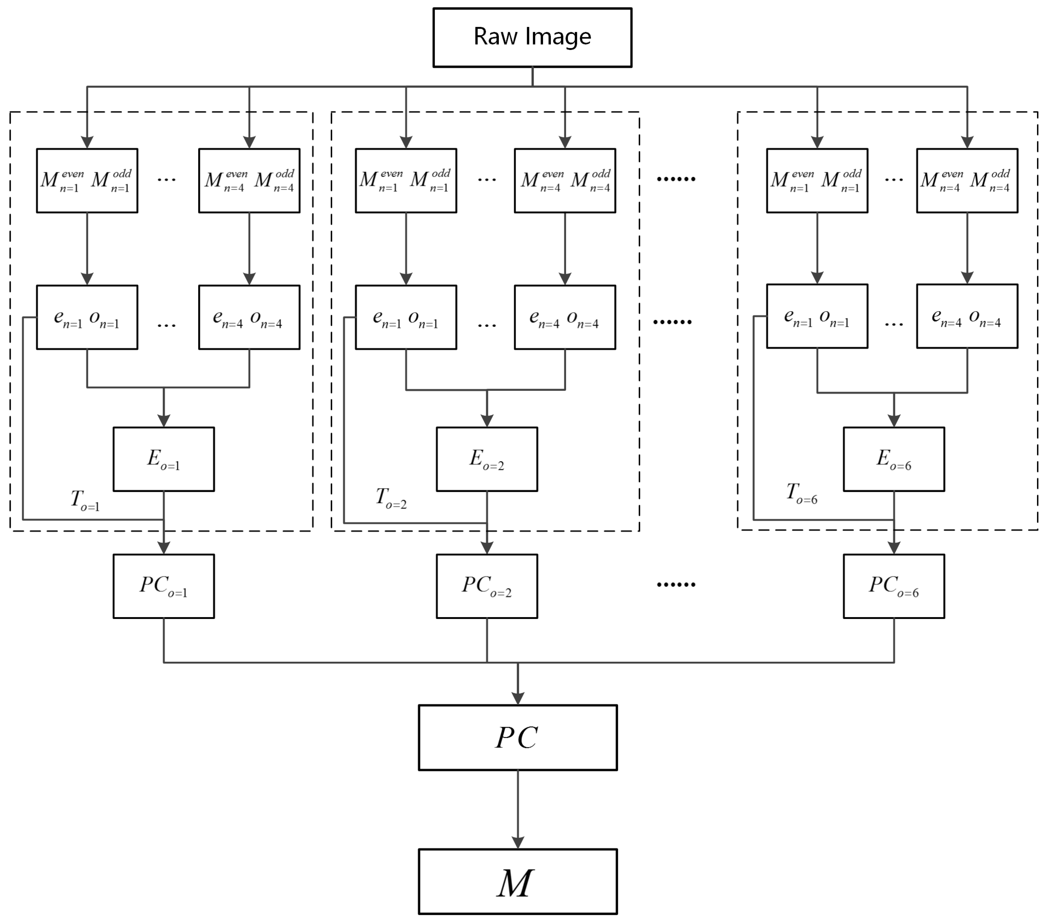
2. Review of the Phase Congruency

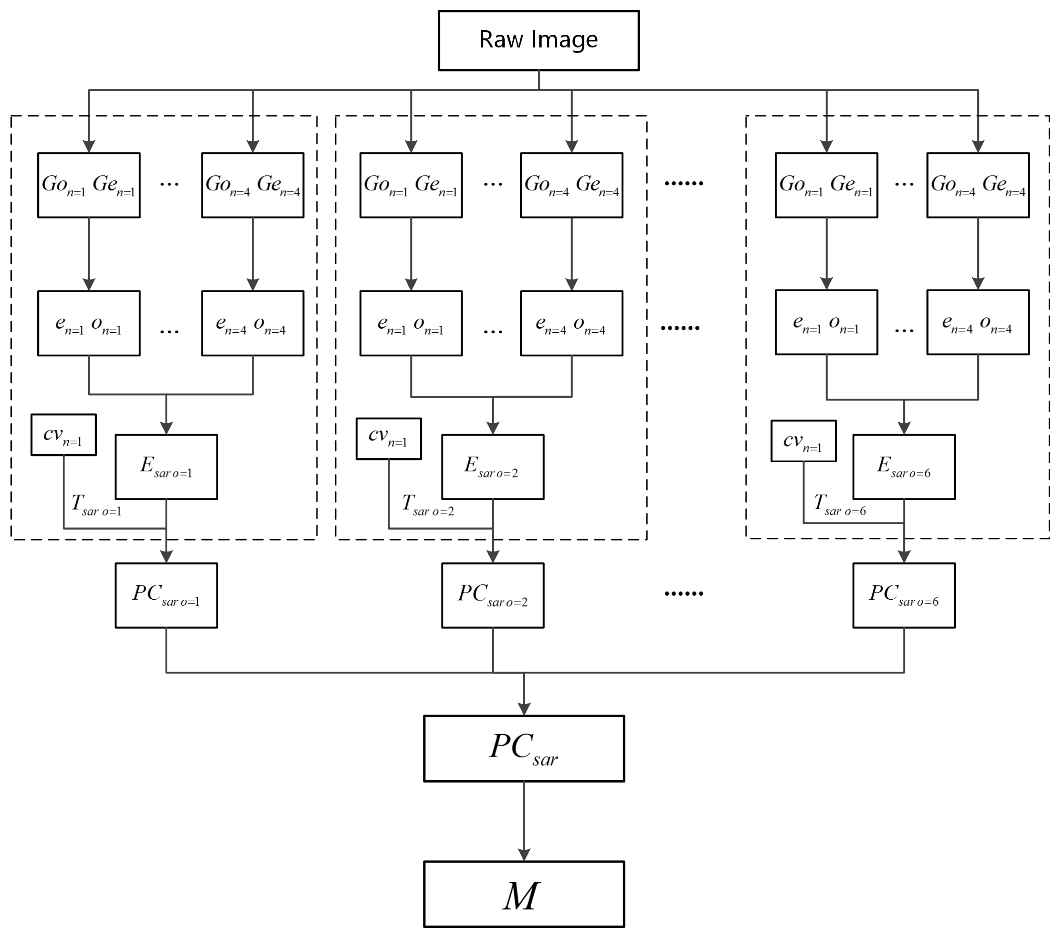
Herein, we briefly review the entire phase congruency procedure to extract edges and corners in optical images. The phase congruency detector consists of three main modules: local energy and phase congruency, noise estimation, edge and corner extraction.

Different from extracting features with the classical gradient-based operators, edges can be perceived at points where the Fourier components are maximally in phase. Figure 1 illustrates the Fourier series of a square waveform and a triangular waveform. For the square waveform, all the Fourier components are sine waves that are exactly in phase at the point of the step at an angle of $0^{\circ }$ or ${180}^{\circ }$. Similarly, for the triangular waveform, the phases of all Fourier components are ${90}^{\circ }$ at its peak [22]. These points are all maximum in phase congruency. Based on these observations, phase congruency becomes a widely-used feature detector.

In practice, Venkatesh and Owens showed in [23] that the local energy model is directly proportional to phase congruency. Hence, peaks in local energy correspond to peaks in phase congruency. Herein, the measure of local energy is calculated by convolving the image with a filter bank of quadrature filters. In order to extend the local energy model to two dimensions, Kovesi calculated local energy at a number of separate orientations and then formed the sum over all orientations [24]. The basic model of 2D phase congruency is given as:

$$PC=\frac{{\displaystyle \sum _o}{E}_o}{{\displaystyle \sum _o}{\displaystyle {\displaystyle \sum _n}}{A}_n+\epsilon },$$

(1)

where n represents the number of scales, o stands for the number of orientations, E is the local energy, $A_n$ is the amplitude, and ε is a small positive value to prevent the expression from becoming unstable when $A_n$ becomes very small. Let $M_n^e$ and $M_n^o$ denote the even and odd symmetric filters in quadrature at a scale n. Then the original image and its Hilbert transform are described as:

$$e\left(x\right)=\sum _{n}I\left(x\right)*M_n^e,o\left(x\right)=\sum _{n}I\left(x\right)*M_n^o,$$

(2)

respectively, where I represents the image intensity, $M_n^e$ and $M_n^o$ denote the even and odd symmetric filters at a scale n, $e\left(x\right)$ represents the convolution of the image with the even symmetric filter, and $o\left(x\right)$ represents the convolution of the image with the odd symmetric filter. Local energy and the amplitude are calculated by:

$$E\left(x\right)=\sqrt{e{\left(x\right)}^2+o{\left(x\right)}^2}$$

(3)

$$\sum _n{A}_n=\sum _n\sqrt{{\left(I\left(x\right)*M_n^e\right)}^2+{\left(I\left(x\right)*M_n^o\right)}^2}$$

(4)

Because the calculation of local energy requires the integration of information over scales, it is reasonable to estimate the noise level across scales. Noise in the optical images can be assumed to be an additive Gaussian noise with a constant power spectrum. Thus, the distribution of each local energy vector over scales will be a 2D Gaussian and the magnitude of the total local energy vector has a Rayleigh distribution [25]. Kovesi argued that the smallest scale filter has the largest bandwidth, and as such, will give the strongest noise response [24]. Consequently, the distribution of the amplitude response from the smallest scale filter pair will be primarily the noise distribution. A robust estimate of noise level is obtained from the median response of the smallest scale filter. Then, T is taken to be the mean of the noise energy response plus some multiple, as follows:

$$T={\mu }_R+k{\sigma }_R,$$

(5)

where T is the noise level, ${\mu }_R$ and ${\sigma }_R$ are the mean and variance of the Rayleigh distribution describing the local energy response of the smallest scale, k is typically in the range two to three. To solve the high-frequency components reduction caused by Gaussian smoothing, Kovesi proposed a weighting function that restrains the response at points where the frequency spread is low [20]. The function is constructed by applying a sigmoid function to the filter response spread value, namely $W\left(x\right)$. Substituting the noise level and the weight function into the basic model of phase congruency, the PC detector reduces the spurious responses and sharpens the localization of features. It is given as:

$$PC(x,y)=\frac{{\displaystyle \sum _o}{W}_o(x,y)⌊E_o(x,y)-T_o⌋}{{\displaystyle \sum _o}{\displaystyle \sum _n}{A}_n+\epsilon },$$

(6)

where $W_o$ represents the weighting function at the oth orientation.

Finally, Kovesi indicated that the principal axis, corresponding to the axis about which the moment is minimized, provides an indication of the orientation. The magnitude of the maximum moment, corresponding to the moment about an axis perpendicular to the principal axis, gives an indication of the significance of the edges [21]. Accordingly, the maximum and minimum phase congruency moments can be directly used to detect the significant edge and corner points. The maximum moment is calculated as the expression below. The flow chart of PC is shown in Figure 2. Further details about phase congruency can be found in [20,21,24].

$$M=\frac{1}{2}\left(\begin{array}{c}{\displaystyle \sum _{\theta }}\left[{\left(P\right(\theta )sin(\theta \left)\right)}^2+{\left(P\right(\theta )cos(\theta \left)\right)}^2\right]\hfill \\ +\sqrt{4{\left({\displaystyle \sum _{\theta }}\left(P\right(\theta \left)sin\right(\theta \left)\right)\left(P\right(\theta )cos(\theta \left)\right)\right)}^2+{\left({\displaystyle \sum _{\theta }}\left[{\left(P\right(\theta \left)cos\right(\theta \left)\right)}^2-{\left(P\right(\theta \left)sin\right(\theta \left)\right)}^2\right]\right)}^2}\hfill \end{array}\right)$$

(7)

3. Methodology

Due to the property of being constant to image contrast and the identification of various types of features, the phase congruency model has been widely used in SAR image processing, such as image registration [26,27], target detection [28], edge detection [29], and image segmentation [30]. However, in these applications, the phase congruency model is applied directly to the raw SAR image or the logarithmic SAR image, which suffers from the effect of the speckle noise. Herein, we propose an improved phase congruency model that is adapted to the multiplicative speckle noise, including the SAR local energy model and a new estimation of noise.

Being similar to the phase congruency model, our proposed SAR-PC model can also be divided into three steps: the SAR local energy model, noise estimation, and edge and corner extraction. The flow chart of SAR-PC is shown in Figure 3.

Step 1: We firstly divide the Gabor filter into two parts—an even-symmetric function and an odd-symmetric function. By calculating the local mean of the even-symmetric and odd-symmetric Gabor processing windows, two ratio responses are obtained. Replacing the convolution of raw image and the quadrature filters by the two ratio values, the SAR local energy model is derived.

Step 2: We explore the relationship between the decision threshold with the coefficient of variation to automatically calculate the noise level. A new estimation of noise level that is adapted to the multiplicative noise is obtained based on the SAR local energy model.

Step 3: Substituting the SAR local energy model and the new noise level into the PC model, the SAR-PC is deduced. Edge responses can be calculated from the max moment of the SAR-PC model.

The principles and implementations of the proposed SAR-PC detector will be described in detail in the following sections.

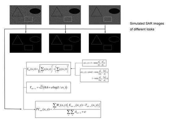
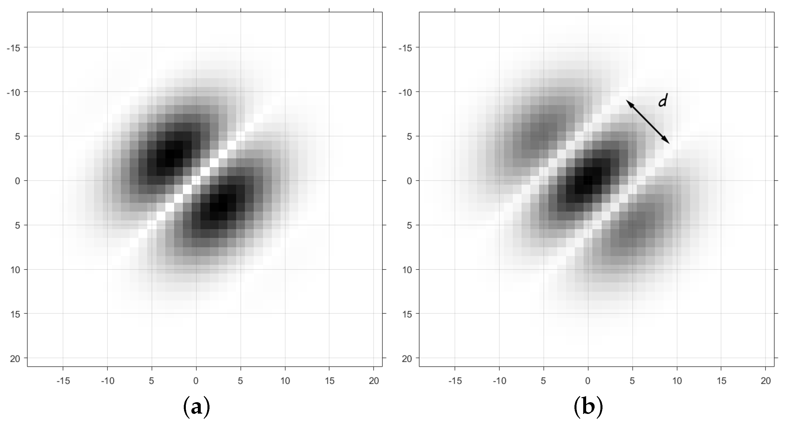
3.1. SAR Local Energy Model

In the calculation of local energy, the convolutions of images and the quadrature filters have a poor result for SAR images due to the multiplicative noise. Herein, the ratio-based detectors are applied to the calculation of local energy. We name it the SAR local energy model.

In the proposed model, the 2D Gabor filters are chosen as the quadrature filters to calculate the local energy. Gabor filters have been widely used in image processing due to their properties of replicating human visual characteristics and modulating the scale and orientation [31]. They are also good edge detectors used in optical images [32]. Whereas the even-symmetric Gabor filter has a non-zero DC component, we eliminate the DC component by subtracting a constant. The even-symmetric and odd-symmetric Gabor filters oriented at an angle θ are given by:

$$G_{even}(x,y)=exp\left[-\frac{x^2+y^2}{2{\sigma }^2}\right]\left[cos\left[\omega (xcos\theta +ysin\theta )\right]-t\right]$$

(8)

$$G_{odd}(x,y)=exp\left[-\frac{x^2+y^2}{2{\sigma }^2}\right]sin\left[\omega (xcos\theta +ysin\theta )\right],$$

(9)

where w represents the frequency of a sinusoidal wave, σ controls the scale of a Gaussian envelope, and t stands for the constant to remove the existing DC component. The reason why we choose Gabor filters instead of Log-Gabor filters is that Gabor filters are more flexible in parameter selection under the comparable performance with Log-Gabor filters. An example of the odd-symmetric and even-symmetric Gabor filters is shown in Figure 4. It is clear that the odd-symmetric function consists of two parts and the even-symmetric function consists of three parts. They are given as follows:

$$\left\{\begin{array}{c}G{o}_1(x,y)=G_{odd}(x,y),xsin\theta -ycos\theta >0\\ G{o}_2(x,y)=-G_{odd}(x,y),xsin\theta -ycos\theta <0\end{array}\right\}$$

(10)

$$\left\{\begin{array}{c}G{e}_1(x,y)=G_{even}(x,y),\left|xsin\theta -ycos\theta \right|<d\\ G{e}_2(x,y)=-G_{even}(x,y),xsin\theta -ycos\theta <-d\\ G{e}_3(x,y)=-G_{even}(x,y),xsin\theta -ycos\theta >d\end{array}\right\},$$

(11)

where d represents the width of the central window shown in Figure 4b. Similar with the GSS detector [6], we replace the rectangle window used in the ROA and the RL detector with the sliding window formed by the even-symmetric and odd-symmetric Gabor filters. Two local means are calculated by convolving these functions with the raw intensities as follows:

$$\begin{array}{c}{\mu }_o^i={\displaystyle \sum _{(x^{\prime },y^{\prime })}}I(x^{\prime },y^{\prime })G{o}_i(x-x^{\prime },y-y^{\prime }),i=1,2\hfill \\ {\mu }_e^j={\displaystyle \sum _{(x^{\prime },y^{\prime })}}I(x^{\prime },y^{\prime })G{e}_j(x-x^{\prime },y-y^{\prime }),j=1,2,3\hfill \end{array}$$

(12)

The original image and its Hilbert transform are described by the two ratio values as:

$$e(x,y)=1-min(\frac{{\mu }_o^1}{{\mu }_o^2},\frac{{\mu }_o^2}{{\mu }_o^1})$$

(13)

$$o(x,y)=min(1-min(\frac{{\mu }_e^1}{2{\mu }_e^2},\frac{2{\mu }_e^2}{{\mu }_e^1}),1-min(\frac{{\mu }_e^1}{2{\mu }_e^3},\frac{2{\mu }_e^3}{{\mu }_e^1})),$$

(14)

respectively. Accordingly, the SAR local energy model and the amplitude are derived by $e(x,y)$ and $o(x,y)$ over scales

$$E_{sar}(x,y)=\sqrt{{\left(\sum _n{e}_n(x,y)\right)}^2+{\left(\sum _n{o}_n(x,y)\right)}^2},$$

(15)

$$\sum _n{A}_n=\sum _n\sqrt{{\left(e_n(x,y)\right)}^2+{\left(o_n(x,y)\right)}^2},$$

(16)

where n represents the scale, and different scale corresponds to different window size of the Gabor function. When extending to two dimensions, we have to take orientation into consideration. The aforementioned Gabor functions are rotated to several orientations, and six directions are used after considering the detection accuracy and computational complexity. The SAR local energy at each orientation is substituted into Equation (6) for the construction of the SAR-PC. Local orientation at each point is obtained by determining the maximum of the SAR local energy of each orientation.

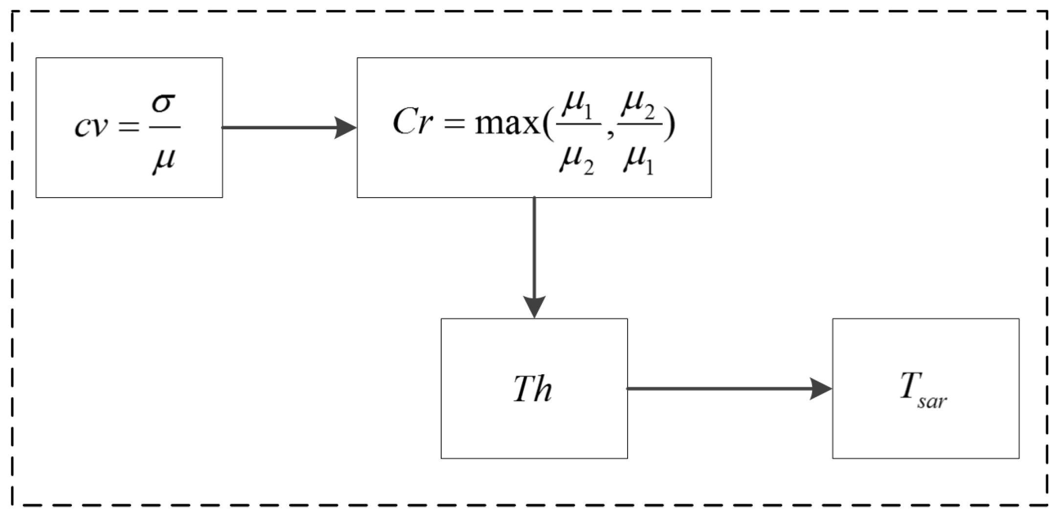
3.2. Noise Estimation

The noise level used in the phase congruency is designed to eliminate the additive noise. Suffering from high frequency components caused by speckle noise, the existing noise level is no longer applicable. It is urgent to propose a new noise estimation for SAR imagery.

The SAR local energy model has theoretically solved the problem of speckle noise; herein, we propose a new estimation of noise level that is adapted to the calculation of SAR local energy. Since we use the ratio values to construct the SAR local energy model, it is reasonable to eliminate the noise response in $e(x,y)$ and $o(x,y)$. The estimation of noise level is changed to an estimation of a decision threshold that can separate true edge points from noise points in the ratio-based detectors. We explore the relationship between this threshold and the coefficient of variation ($cv$) to automatically calculate the decision threshold. The flow chart of noise estimation is shown in Figure 5.

Herein, we typically choose the ROA detector from the ratio-based detectors for simplicity. Speckle results from the interference patterns generated by random scattering from surfaces which are rough on the scale of an optical wavelength [1]. Since the speckle is statistically well-modeled, several models describing the first- and second-order statistics laser speckle patterns have been derived. The most widely recognized model is a stationary multiplicative noise process having negative-exponential first-order statistics and unity variance, which is used in this paper.

Assuming that μ is the average intensity of a homogenous region at coordinate $(x,y)$, the probability density function (pdf) of intensity $I(x,y)$ is defined as:

$$f_L\left(i\right)=\frac{1}{\mathsf{\Gamma }\left(L\right)}{(\frac{\mu }{L})}^{{-L}_{i}L-1}exp(\frac{-iL}{\mu }),$$

(17)

where L is the number of looks, Γ is the gamma function, and i is the intensity. The average and variance of the homogenous region are ${\mu }_L=\mu$ and ${\sigma }_L^2={\mu }^2/L$, respectively. Figure 6 illustrates a processing window of the ROA detector. The processing window consists of two non-overlapped homogenous regions. Its shape and orientation are specified by length l, width w, spacing d, and orientation θ. For the pixel to be detected, two homogenous sub-regions are ${\mathrm{I}}_1$ and ${\mathrm{I}}_2$ , with averages $({\mu }_1,{\mu }_2)$ and variances $({\sigma }_1^2,{\sigma }_2^2)$, respectively. Then, the ratio value can be described as $R=min({\mu }_1/{\mu }_2,{\mu }_2/{\mu }_1)$, and its conditional pdf is given by:

$$p\left(R\right|{\mu }_1/{\mu }_2)=\frac{n\mathsf{\Gamma }\left(2NL\right)}{\mathsf{\Gamma }{\left(NL\right)}^2}[\frac{{({\mu }_1/{\mu }_2)}^{NL}}{{(R^n+({\mu }_1/{\mu }_2))}^{2NL}}+\frac{{({\mu }_2/{\mu }_1)}^{NL}}{{(R^n+({\mu }_2/{\mu }_1))}^{2NL}}]R^{nNL-1},$$

(18)

where $n=1$ for a power image, $n=2$ for an amplitude image, and N is the number of pixels in the homogenous region. The performance of the ROA detector can be discussed as a function of the size of neighborhoods, the number of looks, and the ratio of the mean values [1]. Given a decision threshold $Th$, if $R>Th$, the sample pixel is detected as an edge pixel. The conditional probability of detection ($Pd$) within a boundary between two homogeneous regions of a contrast ratio $Cr=max({\mu }_1/{\mu }_2,{\mu }_2/{\mu }_1)$ is given by:

$$\begin{array}{c}Pd(Th,Cr)=Pr\mathrm{ob}(r<Th\left|Cr\right)={\int }_o^{Th}p\left(r\right|Cr)dr\hfill \\ ={\int }_o^{Th}p\left(r\right|max({\mu }_1/{\mu }_2,{\mu }_2/{\mu }_1\left)\right)dr.\hfill \end{array}$$

(19)

For an image and a fixed size processing window, the value of $NL$ is constant. The relationships among $Pd$, the decision threshold $Th$, and $Cr$ can be deduced from Equation (19). As shown in Figure 7, given a $Pd$, the smaller the $Cr$, the higher the decision threshold $Th$.

The coefficient of variation that is defined as the ratio between the standard deviation and mean of a specific window plays an important role in SAR image analysis [1]. The $cv$ of the point located at the center of the processing window that is shown in Figure 6 is given by:

$$\begin{array}{c}cv=\sigma /\mu \hfill \\ \sigma =\sqrt{{\displaystyle \sum _{i=1}^{2N+N_d}}{(x_i-\mu )}^2/(2N+N_d-1)}\hfill \\ \mu =\left(N{\mu }_1+N{\mu }_2+N_d{\mu }_d\right)/\phantom{\left(N{\mu }_1+N{\mu }_2+N_d{\mu }_d\right)\left(2N+N_d\right)}\left(2N+N_d\right),\hfill \end{array}$$

(20)

where ${\mu }_1$, ${\mu }_2$ are mean values of two homogeneous regions, respectively, and ${\mu }_d$ is the mean of the space. N and $N_d$ are the number of pixels in these regions, respectively. In the calculation of $cv$, the space is negligible because it can be divided into two parts that belong to the adjacent homogenous regions. Then, the relationship between $cv$ and $Cr$ is derived as (details can be seen in Appendix A):

$$cv=2\sqrt{\frac{(N^{\prime }-1)(C{r}^2+1)}{L{N}^{\prime }(2N^{\prime }-1){(Cr+1)}^2}+\frac{N^{\prime }{(Cr-1)}^2}{2(2N^{\prime }-1){(Cr+1)}^2}},$$

(21)

where $N^{\prime }=N+\frac{N_d}{2}$. The plot of $Cr$ varying with $cv$ is shown in Figure 8 for different neighborhood sizes. Combining with the conclusion obtained from Figure 7, we deduce that the bigger the $cv$, the bigger the $Cr$, and the smaller the decision threshold $Th$.

Wei demonstrated in [33] that when $Th$ is smaller than 0.6, the probability of false alarm (PFA) is close to 0, and hence PFA is not sensitive to threshold $Th$. Considering the variation of $Pd$ with $Th$, the expected change range of $Th$ is supposed to be $[0.6,1]$. When the $cv$ is large, the decision threshold in these regions should vary slowly with the $cv$. The expression of the decision threshold $Th$ is deduced as follows:

$$Th=0.6+alog(1/cv),$$

(22)

where a is a shape parameter that controls the rate of variation. Although the formula of $Th$ is derived by the ROA model, the relationship between $cv$ and $Th$ is also adapted in the ratio-based detector using Gabor windows, because the Gaussian shape has slight impact on the variation between $cv$ and $Cr$. Hence, Equation (22) can be directly applied after modifying the shape parameter.

Local energy integrates the information over many scales, so we need to compute the noise response over scales as well. Kovesi argued that the smallest scale filter has the largest bandwidth, and so gives the strongest noise response [24]. To compute the noise level that can eliminate the noise response, the $cv$ of the smallest scale filter is used. The decision threshold is given as:

$$Th=0.6+alog(1/c{v}_s),$$

(23)

where s is the index of the smallest scale filter. The threshold that separates true edge points from noise points is designed for the response of $e(x,y)$. Since the response of $o(x,y)$ can be regarded as the minimum of two responses of $e(x,y)$, the threshold of $o(x,y)$ can be derived same as $Th$. The final noise level at oth orientation is given as:

$$T_{sar-o}=\sqrt{T{h}^2+T{h}^2}.$$

(24)

Substituting the SAR local energy model and the new noise estimation into the PC operator, we modify the expression for SAR phase congruency to the following:

$$P{C}_{sar}(x,y)=\frac{{\displaystyle \sum _o}{W}_o(x,y)⌊E_{sar-o}(x,y)-T_{sar-o}(x,y)⌋}{{\displaystyle \sum _o}{\displaystyle \sum _n}{A}_{sar-n}+\epsilon }.$$

(25)

4. Experimental Results

Although the SAR-PC is a robust feature detector, the problem that we discuss here only concentrates on the detection of edges features, including both step edges and roof edges. Consequently, the maximum moments of the SAR-PC detector and PC detector are used to detect edges. For the PC detector, if it is used directly, we name it the PC detector and if it is used after taking the logarithm of the raw image, we name it the Log-PC detector. The two patterns are both compared. Moreover, some state-of-the-art ratio-based edge detectors are also compared, including the RBED and GSS detectors for step edges, and the RL detector for roof edges. The performances of these detectors are evaluated on both simulated SAR images and satellite SAR images. For the simulated SAR images, ROC curves are used to evaluate the detectors. For satellite SAR images, quantitative comparisons are difficult because the ground truth (GT) maps do not exist for real-world images. We compare the visual effects among these detectors.

4.1. Parameter Settings

For fairness, all of the detectors use the same post-processing method, including the nonmaximum suppression and the hysteresis thresholding. The PC detector used in the experiment follows the parameter settings suggested by Kovesi in [21]. The local energy information is obtained using two-octave bandwidth filters over four scales and six orientations. The wavelength of the smallest filters is three pixels, and the scaling between filters is two. For our SAR-PC detector, the parameters are chosen from the parameters below:

$$\left\{\begin{array}{c}{\sigma }_1=1.5,{\sigma }_{i+1}/{\sigma }_i=1.4,i=1,2,3\\ {\omega }_i=1.8/{\sigma }_i;i=1,2,3,4\\ a=0.25\end{array}\right\},$$

(26)

where σ and ω represent the parameters of Gabor wavelets, and a stands for the shape parameter. Actually, it should be noted that the response of $o(x,y)$ can be regarded as the minimum of two responses of $e(x,y)$. In the experiment, we multiply the $o(x,y)$ by a weight value h as follows:

$$o^{\prime }(x,y)=ho(x,y).$$

(27)

We found that a weight h value of 1.5 was good for the following experiments. Other parameters are the same with the PC detector. For the RBED detector, the parameters were chosen from the following parameter space:

$$\left\{\begin{array}{c}\alpha =2,3,4\\ \beta =3,3.5,4.5\\ {\sigma }_{\left|\right|}=2.5,3,4\\ l_{\left|\right|}=1,2,3\end{array}\right\}.$$

(28)

For the GSS detector, the parameters follow the parameter space as:

$$\left\{\begin{array}{c}\alpha =2,3,4\\ \beta =\frac{\mathsf{\Gamma }(2\alpha -1)}{2^{2\alpha -1}{\mathsf{\Gamma }}^2\left(\alpha \right)}\left\{2,3,...10\right\}\\ {\sigma }_x=\frac{1}{\sqrt{\pi }}\left\{5,7,...21\right\}\end{array}\right\}.$$

(29)

For the RL detector, the parameters are taken from the following parameter space:

$$\left\{\begin{array}{c}w=7,11,15\\ l=w\end{array}\right\},$$

(30)

where w represents the width of the processing window, and l stands for the length of the processing window. Moreover, the thresholds that are used in the hysteresis thresholding have a significant influence on the detection performance. All of the aforementioned detectors take the varying thresholds as follows:

$$\left\{\begin{array}{c}{t}_{low}=0.06+0.02p_1,p_1=1,2,...,14\\ t_{high}=t_{low}+0.02p_2,p_2=1,2,...,(0.4-t_{low})/0.02\end{array}\right\}.$$

(31)

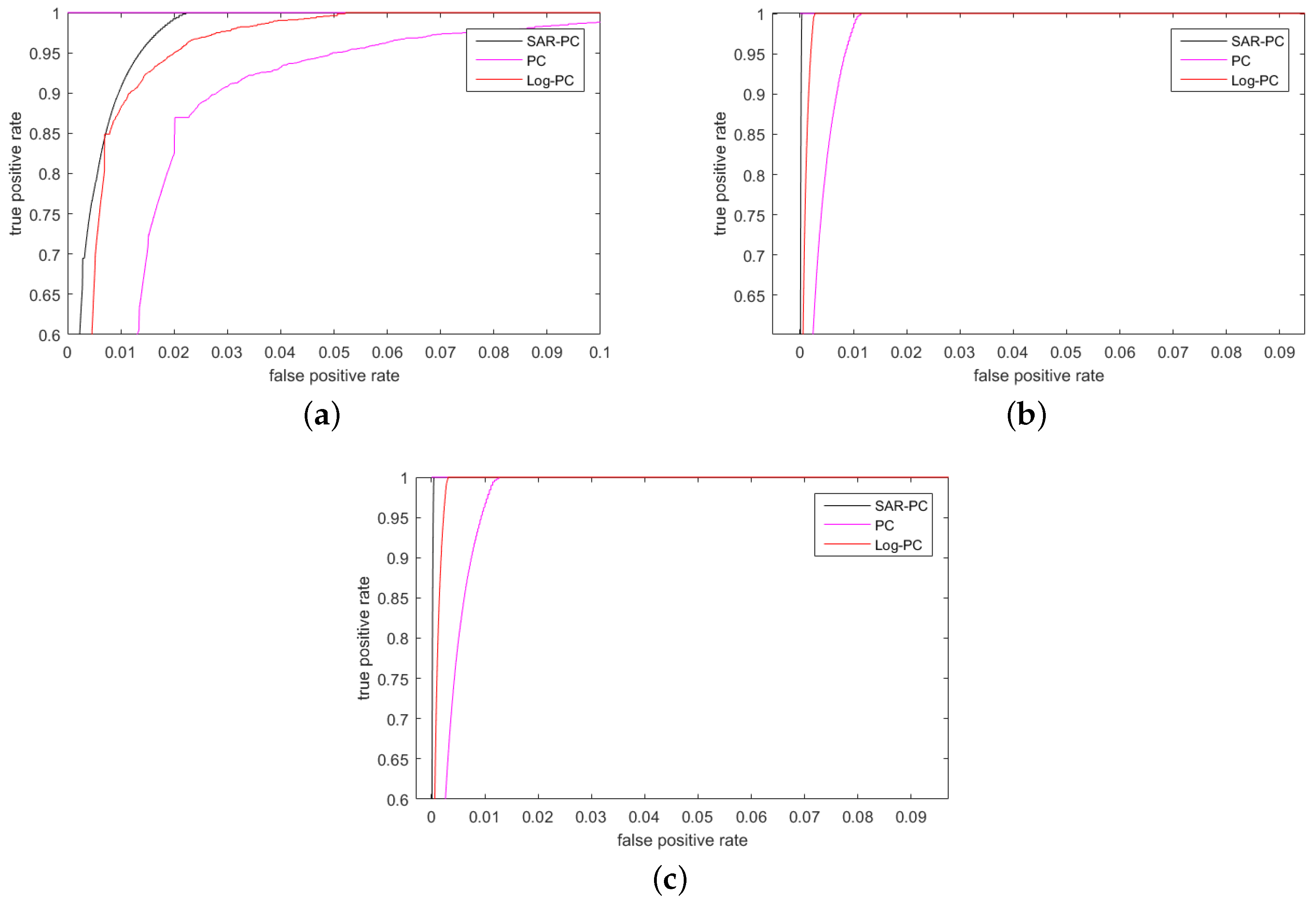
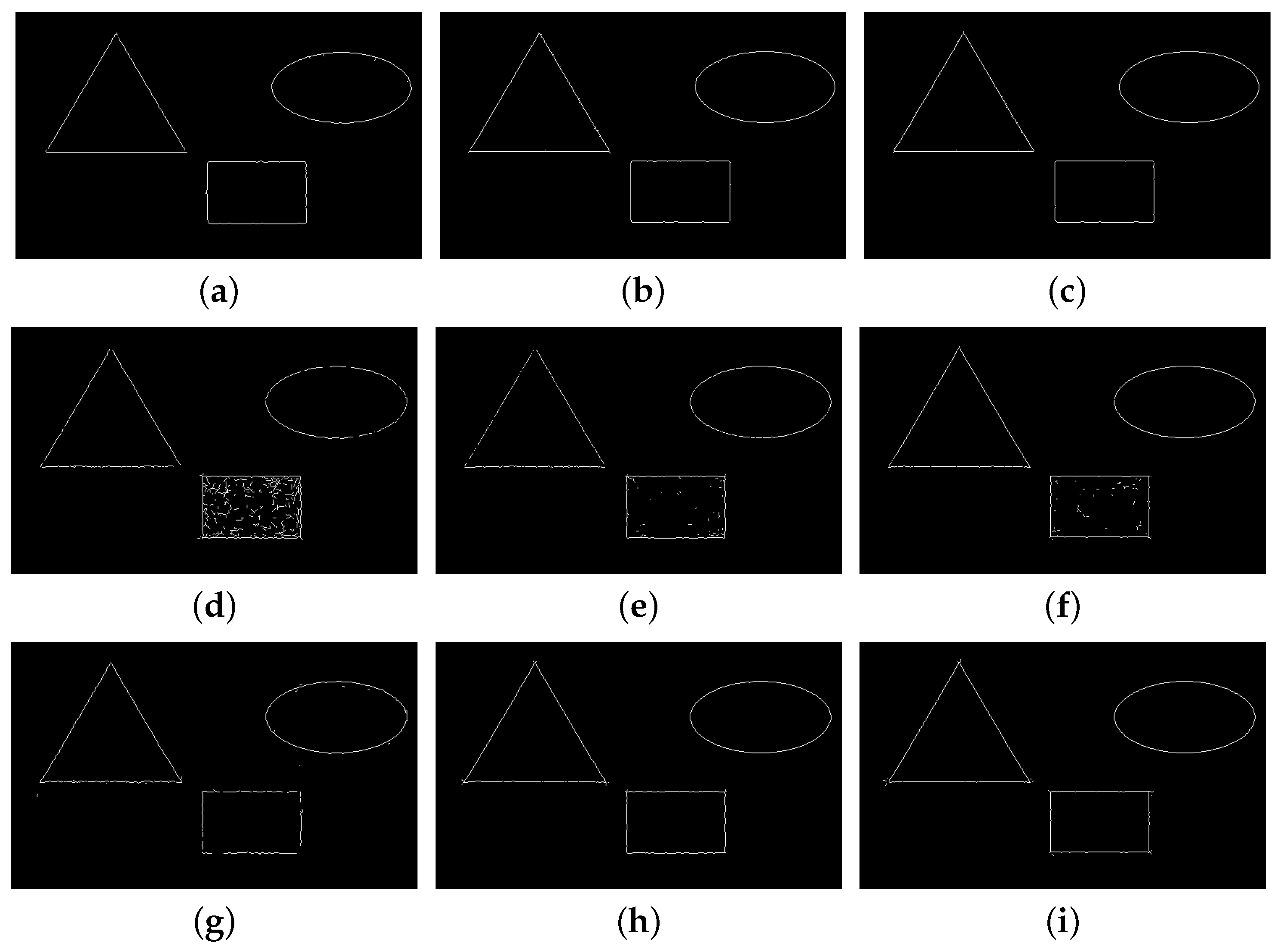
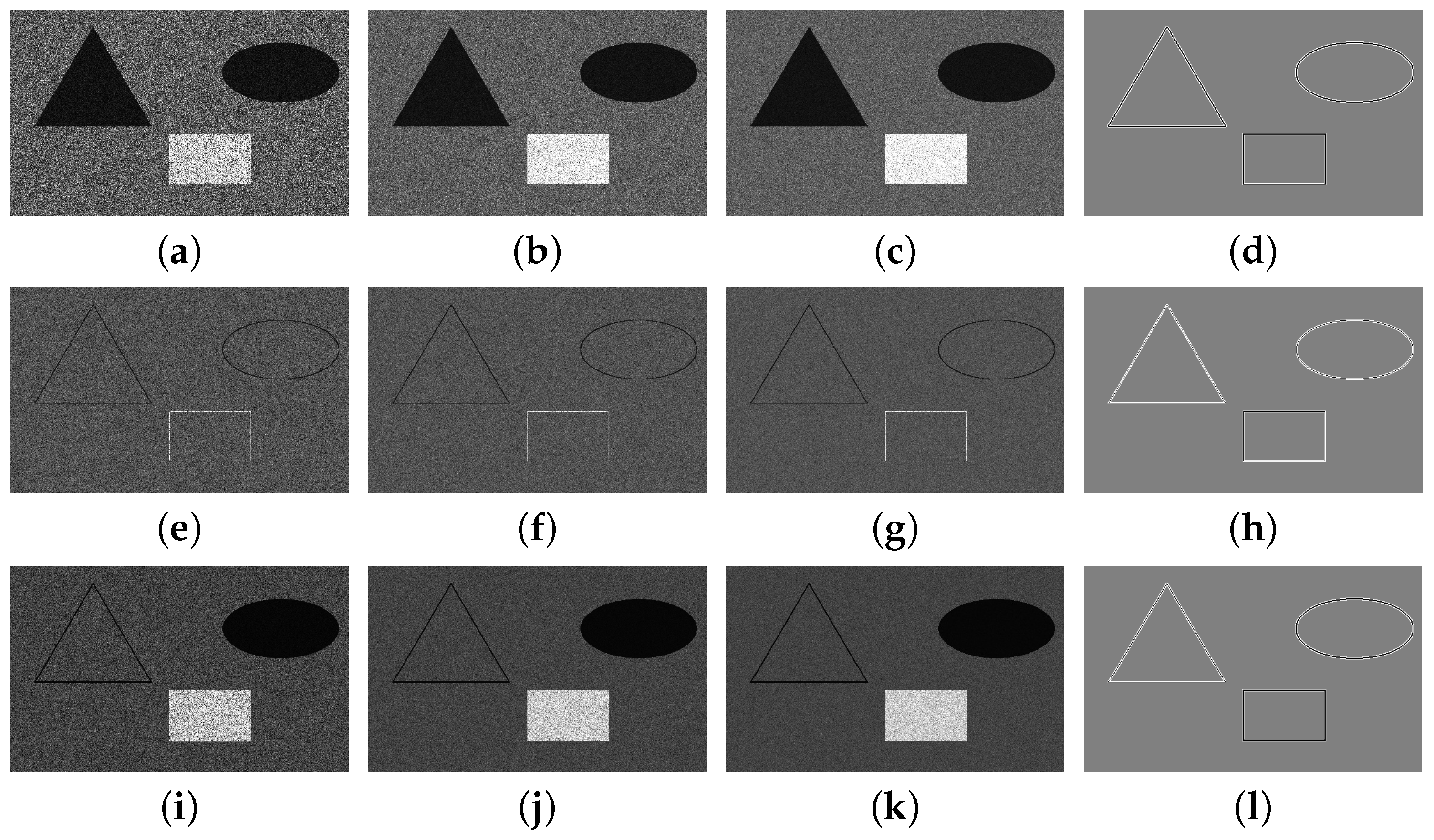
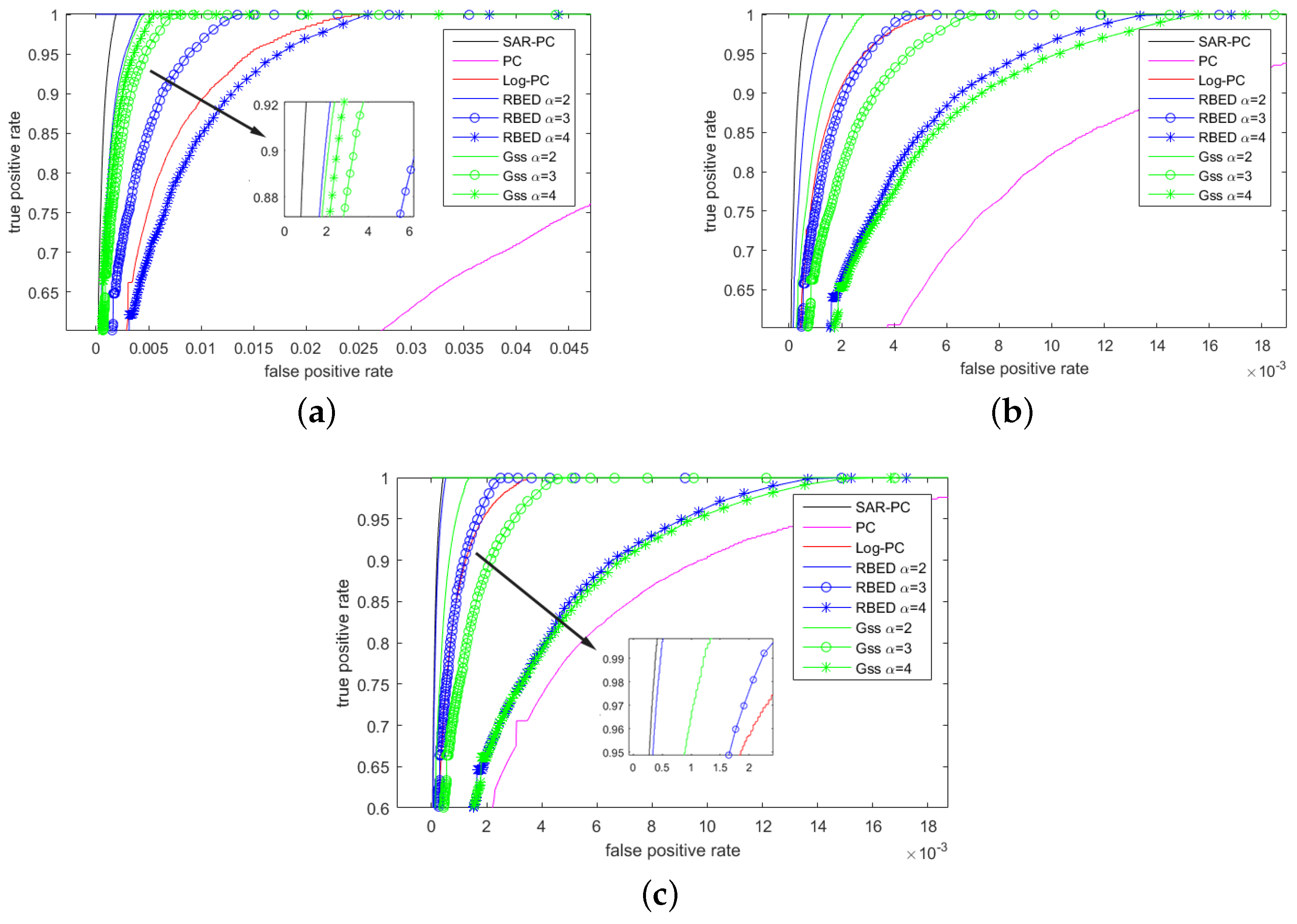
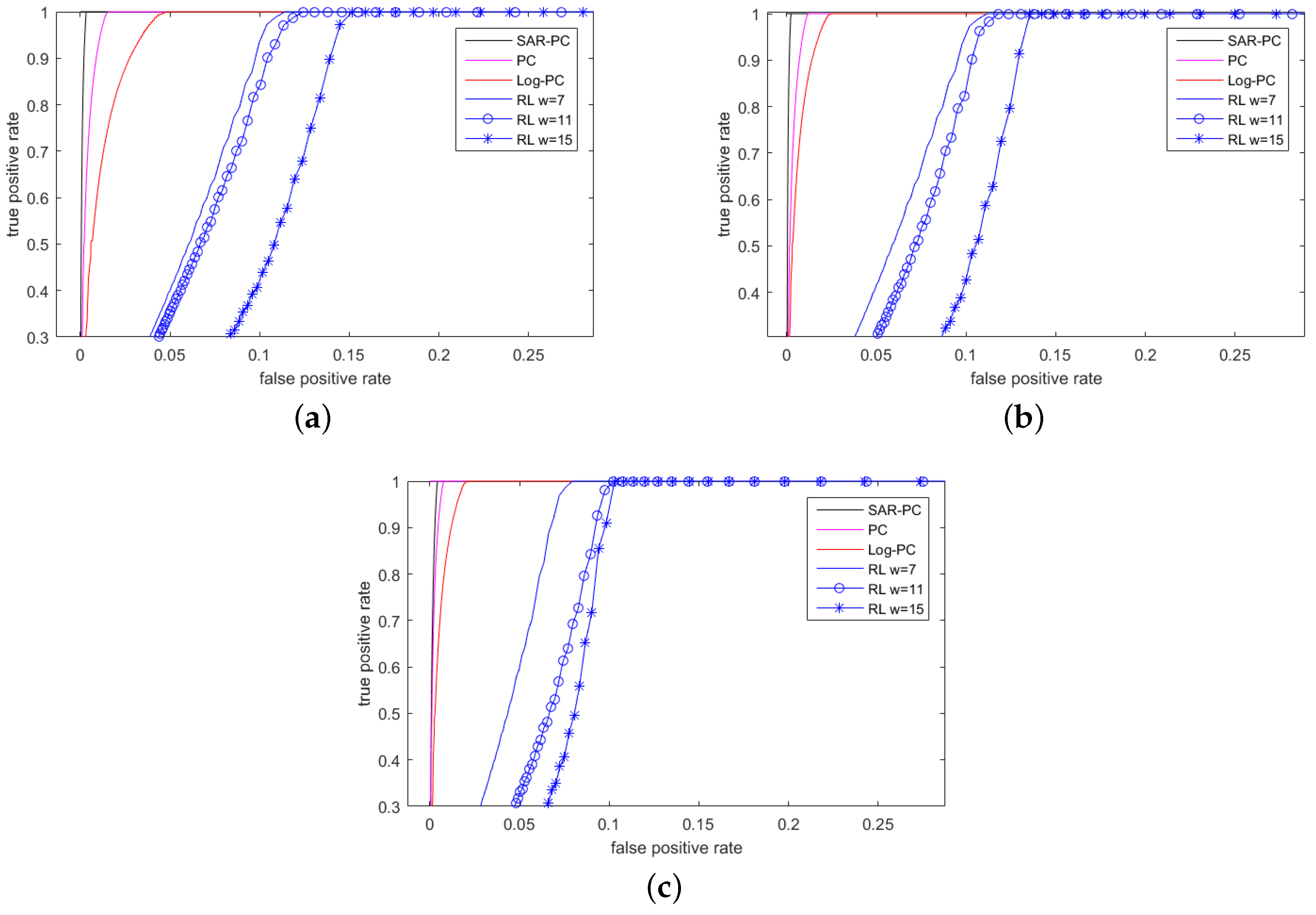
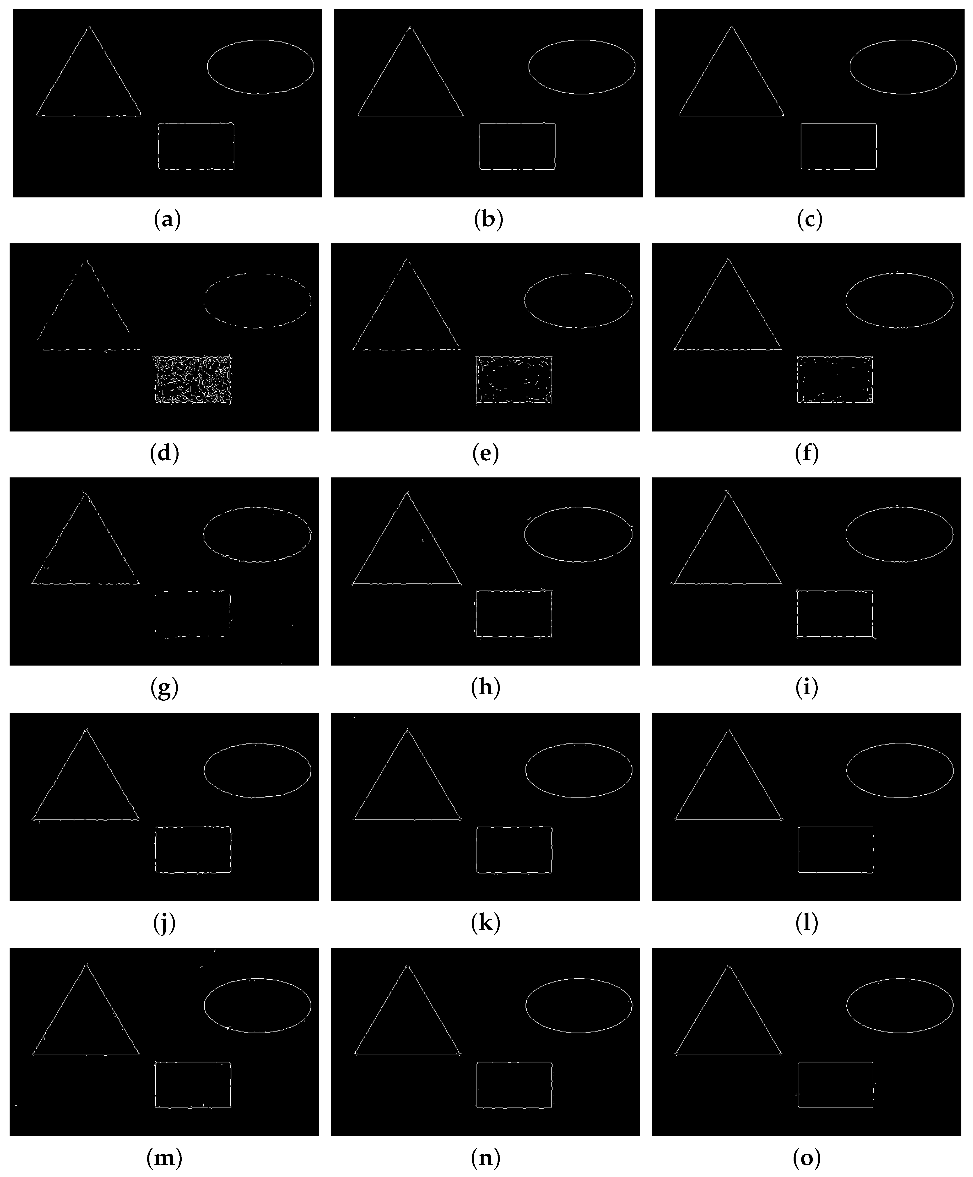
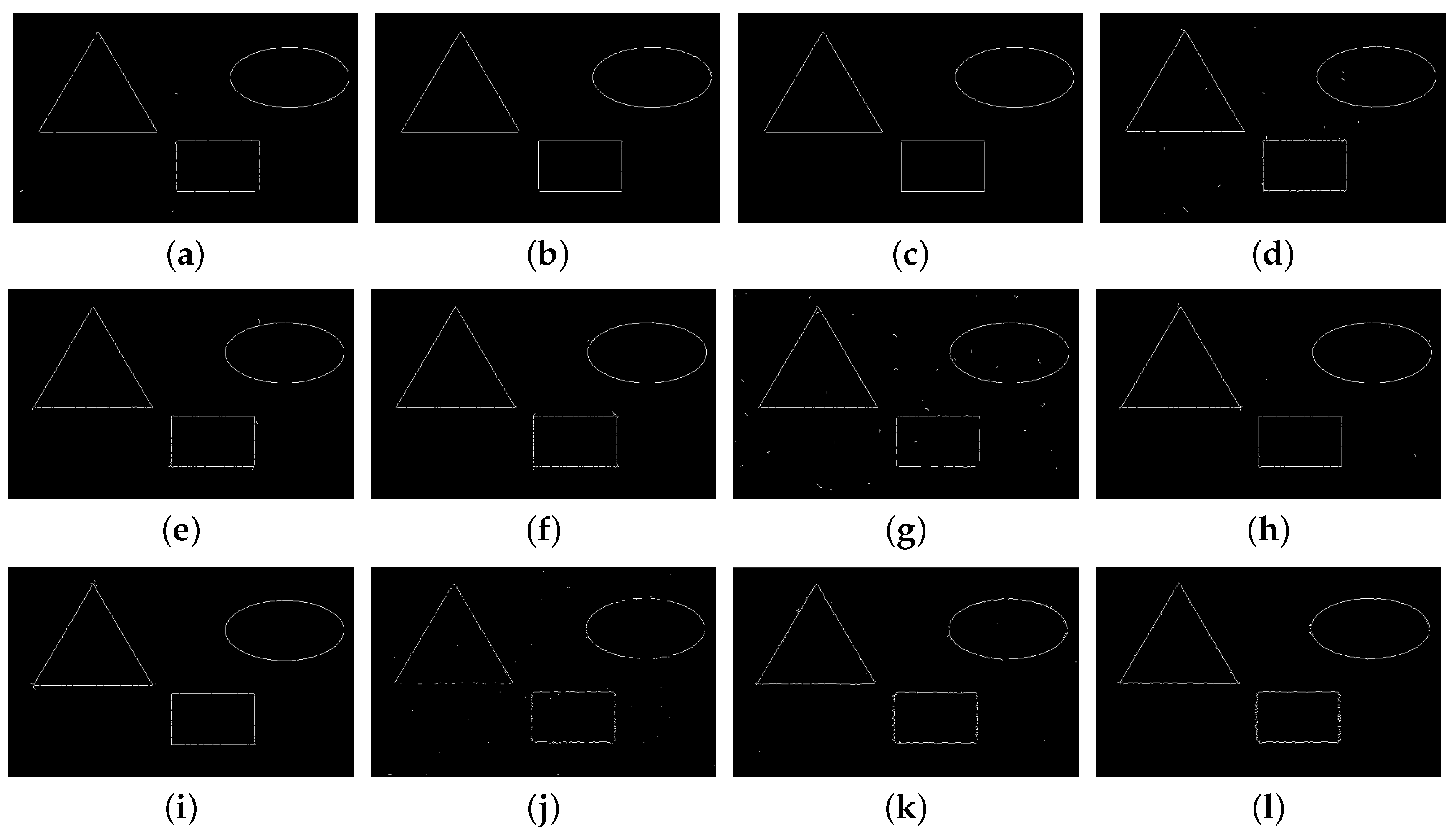
4.2. Comparison on Simulated SAR Images

To compare the detection performance of these detectors on both step edges and roof edges, we simulate three categories of synthetic SAR images. The first category only contains step edges, shown in Figure 9a–c. Based on these simulated images, the SAR-PC detector, PC detector, Log-PC detector, RBED detector, and GSS detector are compared. The second category only contains roof edges, shown in Figure 9e–g. We compare the RL detector with the SAR-PC, PC, Log-PC detectors. There exist both step edges and roof edges in the third category, shown in Figure 9i–k. Consequently, only the SAR-PC, PC, and Log-PC detectors are compared.

The synthetic SAR images are simulated by one polygon image with multiplicative noise under different numbers of looks. Their GT maps are shown in Figure 9d, h, l. The black pixels in GT maps indicate edge pixels, and non-edge pixels are marked in gray. Pixels that are in the $3\times 3$ neighborhood of a black pixel are labelled as white. The GT map is divided into three regions, including an edge region, a non-edge region, and a match region. They correspond to the black pixels, the gray pixels, and the white pixels, respectively. If a detector reports an edge pixel in the edge region or match region, then it is counted as a True Positive ($TP$). If a detector reports an edge pixel in a non-edge region, then it is counted as a False Positive ($FP$). If a detector reports a non-edge pixel in the edge region, then it is counted as a False Negative ($FN$). If a detector reports a non-edge pixel in a non-edge region, then it is counted as a True Negative ($TN$) [34]. $n_{TP}$, $n_{TN}$, $n_{FN}$, and $n_{FP}$ are the number of $TP$, $TN$, $FN$, and $FP$ pixels, respectively. We use the True Positive Rate ($TPR$) and False Positive Rate ($FPR$) to evaluate the performance for detectors at each parameter setting. The $TPR$ and $FPR$ are given as follows:

$$TPR=\frac{n_{TP}}{n_{TP}+n_{FN}},FPR=\frac{n_{FP}}{n_{FP}+n_{TN}}.$$

(32)

Hence, when a detector runs in its parameter space, the closer the receiver operating characteristic (ROC) curve is to the top left side, the better the detection performance of the detector [35].

The ROC curves of the detectors in the parameter spaces for three categories of the simulated SAR images are shown in Figure 10, Figure 11 and Figure 12, respectively. Figure 13, Figure 14 and Figure 15 illustrate the edge binary maps of these detectors with the best parameter settings of the ROC curves.

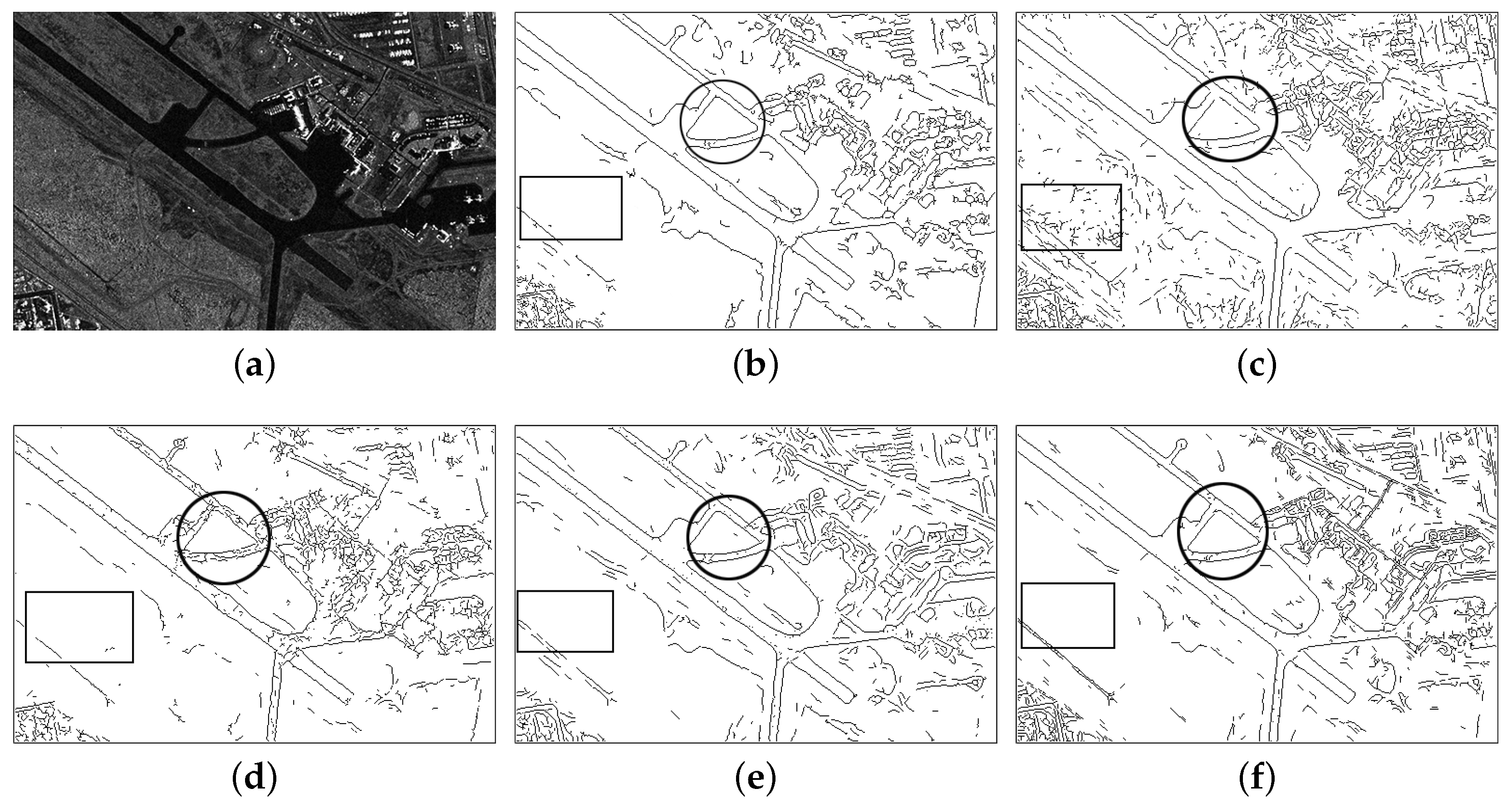
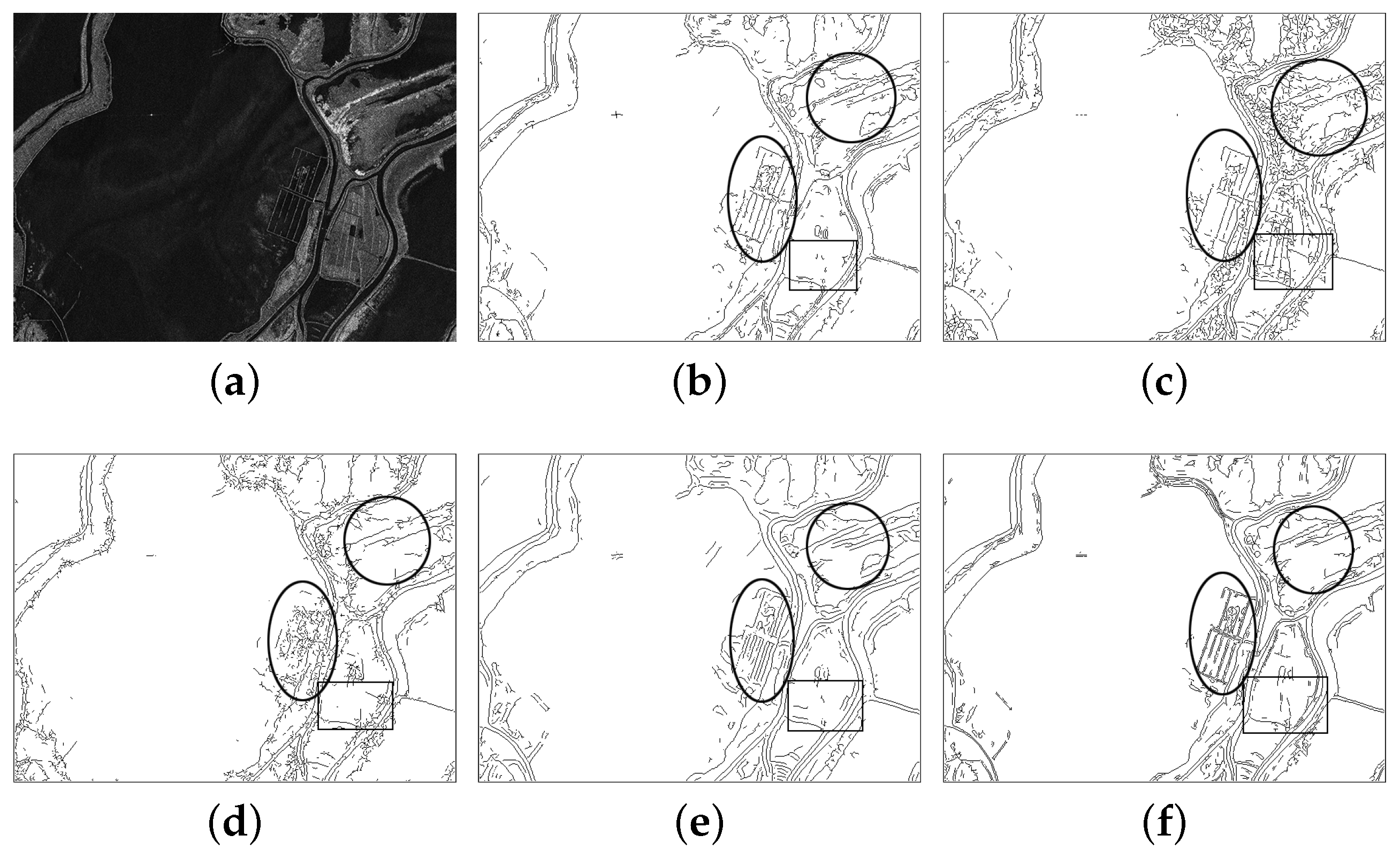
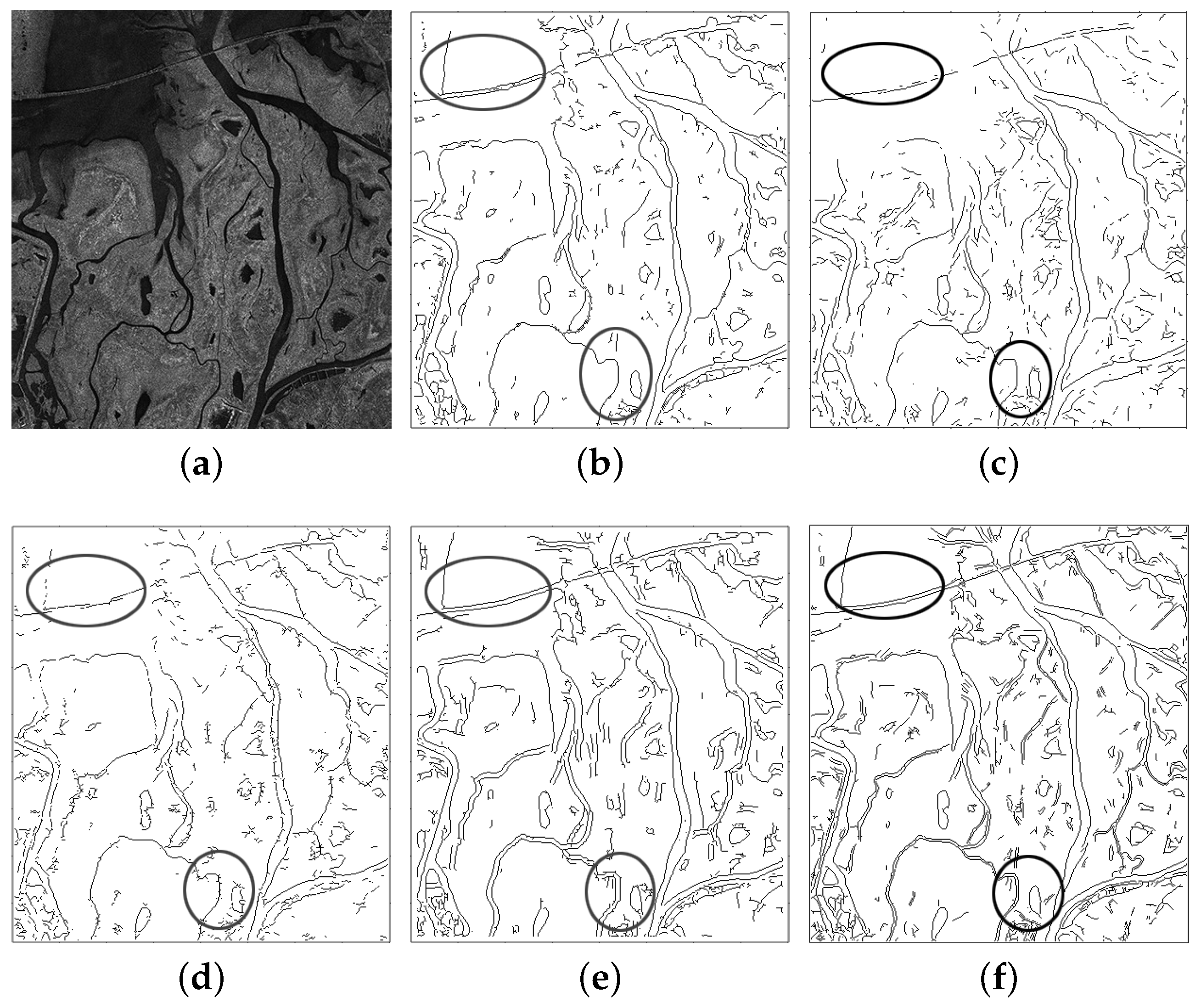
4.3. Comparison on Satellite SAR Images

Finally, satellite SAR images are applied in the experiment. We choose three amplitude-format SAR images to evaluate these detectors, including two images from the GF-3 satellite (a Chinese satellite launched on 10 August 2016) and one image from the TerraSAR-X SAR instrument. The first image was imaged by the Ultra-Fine Stripmap mode with HH polarization (Figure 16a). It is an integrated area of farmland and rivers with 3-m resolution ($600\times 446$ pixels). The second image was imaged by the SpotLight mode with VV polarization (Figure 17a). It illustrates some branches of a small river with 1-m resolution ($400\times 441$ pixels). The third image was imaged by the SpotLight mode with HH polarization (Figure 18a). It is a repository of out-of-service aircrafts ($609\times 758$ pixels). In this experiment, we set the same parameters used in the simulated experiment for the PC detector and the proposed SAR-PC detector, $\left\{\alpha =2,\beta =3,{\sigma }_{\left|\right|}=2.5,l_{\left|\right|}=1\right\}$ for the RBED detector and $\left\{\alpha =2,\beta =1,{\sigma }_x=3\right\}$ for the GSS detector. Since we need to evaluate the robustness of the detectors to speckle noise, we do not apply a despeckling filter to the real-world images in the preprocessing phase. The edge binary maps of these detectors are shown in Figure 16b–f, Figure 17b–f and Figure 18b–f.

5. Discussion

5.1. Discussion On Simulated SAR Images

In the previous section, three categories of synthetic SAR images were demonstrated in order to compare the performance of the detectors on both step edges and roof edges. Meanwhile, in order to evaluate the robustness of our proposed detector to speckle noise, synthetic images of different numbers of looks were also compared.

The first category contains only step edges, shown in Figure 9a–c. There are three polygons in these images. It is obvious that the one-look simulated SAR image has the strongest multiplicative noise, followed by the three-look simulated SAR image. Based on the simulated images, the SAR-PC, PC, Log-PC, RBED, and GSS are compared. Figure 10 illustrates the ROC curves of these detectors. We can see from the ROC curves that our proposed SAR-PC detector gives the best detection performance, not only on the one-look synthetic SAR image, but also on the three-look and six-look synthetic SAR images. The RBED and GSS detectors are the state-of-the-art ratio-based detectors for extracting step edges in SAR images, so they also yield good results on step edges. However, the PC detector fails to detect robust edge responses, especially on the one-look simulated SAR image. Edge binary maps of the SAR-PC, PC, Log-PC, RBED $\alpha =2$, and GSS $\alpha =2$ detectors are shown in Figure 13. As shown in Figure 13a–c, the proposed SAR-PC detector extracts accurate and consecutive edge maps for all three simulated SAR images, proving a reliability to eliminate the effect of speckle noise. The RBED and GSS detectors also yield relatively good results, but they detect a few false edge pixels on the one-look synthetic SAR image. For the PC detector, we can see from Figure 13d–f that it extracts many false maxima in the rectangle area. Because the noise level used in the PC detector is the same for all pixels, the noise response caused by the random high frequency components of the speckle noise in the rectangle area cannot be eliminated by this noise level, resulting in many false edge pixels. The Log-PC detector yields better results than the PC detector, but it also fails to extract a consecutive edge response for the one-look simulated SAR image. Even though the speckle noise is statistically well modeled as a stationary multiplicative process having negative-exponential first-order statistics and unity variance [1], the logarithm of speckle noise cannot be simply assumed as a Gaussian with a constant power spectrum. So, the noise estimation of the Log-PC detector is also not adapted to speckle noise.

The second category only contains roof edges, shown in Figure 9e–g. We compare the RL detector with the SAR-PC, PC, and Log-PC detectors. Figure 11 illustrates the ROC curves of these detectors. It is clear that the proposed SAR-PC detector gives the best performance, followed by the PC detector and the Log-PC detector. The RL detector gives the worst performance, because the rectangle window functions used in the RL detector are not good 2D smoothing filters. Strong speckle in SAR images makes the local mean functions using a rectangle window contain some unwanted high frequency components, resulting in false edge pixels [6]. Edge binary maps of the SAR-PC, PC, Log-PC, and RL $w=7$ detectors are shown in Figure 14. The proposed SAR-PC detector yields robust edge responses for all three simulated SAR images, proving its robustness to speckle noise, shown in Figure 14a–c. For the PC, Log-PC, and RL detectors, many false edge pixels are extracted on the one-look simulated SAR images. They all extract relatively good responses on the six-look simulated SAR images, since the effect of speckle noise is weak.

There exist both step edges and roof edges in the third category, shown in Figure 9i–k. The RBED, GSS, and RL detectors have their limits because their design objectives are only seeking to localize step edges or roof edges. Consequently, only the SAR-PC, PC, and Log-PC detectors are compared. Figure 12 illustrates the ROC curves of these detectors. The proposed SAR-PC detector gives the best performance, followed by the Log-PC detector. Edge binary maps of the SAR-PC, PC, and Log-PC detectors are shown in Figure 15. The SAR-PC detector extracts robust and accurate edge responses for all three simulated images. The PC detector has the same problem mentioned in the first category. It detects many false edge pixels in the rectangle area. The Log-PC does not have this phenomenon, since the logarithm of the simulated SAR image reduces the high frequency components of speckle noise. However, the PC detector and the Log-PC detector both failed to detect a consecutive edge response on the one-look synthetic SAR image.

The three categories of simulated SAR images all have the same size ($561\times 341$ pixels), so we compare the running time of each detector on one simulated SAR image. Since the RBED, GSS, and RL detectors need to run in its parameter space, we average the running time of these detectors. The time costs are given in

Table 1. Running time of each detector.

Detectors:	RBED	GSS	RL	PC	Log-PC	SAR-PC
Time (s)	0.22	0.25	0.15	0.85	0.85	0.92

. Because the SAR-PC, PC, and Log-PC detectors combine the results of different scales, the running time is more than the ratio-based detectors.

5.2. Discussion On Satellite SAR Images

Satellite SAR images are also used to evaluate the performance of these detectors. We compare the SAR-PC, PC, Log-PC, RBED, and GSS detectors in the experiment. The real-world images are more complex than the simulated images. They contain many objects and complex scenes, including water, farmlands, buildings, and roads. Since the ground truth maps do not exist for real-world SAR images, we can only use the subjective evaluation. Besides, sometimes it is difficult to distinguish step edges and roof edges in the real-world images, such as rivers and roads. We consider that roof edges stand for lines that have a width less than four pixels.

Edge binary maps of these detectors are shown in Figure 16, Figure 17 and Figure 18. From the detection results, we can see that the proposed SAR-PC detector finds edges appearing at the area with heavy noise (see the left ellipses marked in Figure 16 and Figure 17). Edge responses detected by the SAR-PC detector have better continuity and smoothness, shown in Figure 16b, Figure 17b and Figure 18b. We also find that the edge binary maps obtained by the SAR-PC detector show a good integrity for closed regions, such as lakes (see the right ellipses marked in Figure 16 and Figure 17), airports (see the ellipse marked in Figure 18). The RBED and GSS detectors can extract good results when detecting step edges, but result in a bilateral response of a roof edge, such as the small river shown in the right ellipse marked in Figure 17. According to the aforementioned definition of roof edges, this river is regarded as a roof edge. Consequently, the results of RBED and GSS detectors are not suitable for this situation. Moreover, the SAR-PC, Log-PC, RBED, and GSS detectors all miss a few edge pixels in the low contrast area (see the rectangles marked in Figure 16 and Figure 18). While the PC detector detects both a few true edge pixels and some false edge pixels. Because the PC detector uses the same noise level for all points and it cannot separate points of low contrast from noise points in the homogenous region, both noise points and edge points of low contrast are reserved. For the RBED and GSS detectors, edge responses of points in the low contrast region are much smaller than points in the high contrast region, and therefore the points of low contrast are easily excluded after post-processing. For the SAR-PC detector, even though the noise estimation is adapted to every point, the noise level of points in the low contrast region is relatively higher than points in the high contrast region. Consequently, points of low contrast are likely to be eliminated. How to reserve edge pixels in the low contrast region is a question to be studied in the future.

We also compare the running time of each detector on the satellite SAR images. The time costs of the first satellite SAR image ($446\times 600$ pixels) are given in

Table 2. Running time of each detector.

Detectors:	RBED	GSS	PC	Log-PC	SAR-PC
Time (s)	0.30	0.23	1.29	1.29	1.34

.

6. Conclusions

In this paper, an improved phase congruency detector for SAR edge detection is proposed. Aiming at solving the problems of the identification of different types of features and the speckle noise reduction, we combine the ratio-based detectors and the phase congruency. Replacing the convolution of image and the quadrature filters by the two ratio values calculated by the odd-symmetric and even-symmetric Gabor windows, the SAR local energy model is derived. In addition, a new noise estimation is built for the multiplicative speckle noise. Exploring the relationship between the decision threshold and the coefficients of variation, the noise level is automatically calculated. Substituting the SAR local energy model and the new noise level into the phase congruency model, SAR-PC is derived. The experimental results show that the proposed SAR-PC detector gives good detection performance. The edge response extracted by the SAR-PC detector is robust to speckle noise, and it provides a good continuity and integrity.

References

1. Touzi, R.; Lopes, A.; Bousquet, P. A statistical and geometrical edge detector for SAR images. IEEE Trans. Geosci. Remote Sens. 1988, 26, 764–773. [Google Scholar] [CrossRef]
2. Amirmazlaghani, M.; Amindavar, H.; Moghaddamjoo, A. Speckle suppression in SAR images using the 2-D GARCH model. IEEE Trans. Image Process. 2009, 18, 250–259. [Google Scholar] [CrossRef] [PubMed]
3. Bovik, A.C. On detecting edges in speckle imagery. IEEE Trans. Acoust. Speech Signal Process. 1988, 36, 1618–1627. [Google Scholar] [CrossRef]
4. Ganugapati, S.; Moloney, C. A ratio edge detector for speckled images based on maximum strength edge pruning. In Proceedings of the 1995 International Conference on Image Processing, Washington, DC, USA, 23–26 October 1995; Volume 2, pp. 165–168.
5. Fjortoft, R.; Lopes, A.; Marthon, P.; Cubero-Castan, E. An optimal multiedge detector for SAR image segmentation. IEEE Trans. Geosci. Remote Sens. 1998, 36, 793–802. [Google Scholar] [CrossRef]
6. Shui, P.L.; Cheng, D. Edge detector of SAR images using Gaussian-Gamma-shaped bi-windows. IEEE Geosci. Remote Sens. Lett. 2012, 9, 846–850. [Google Scholar] [CrossRef]
7. Wei, Q.R.; Feng, D.Z. An efficient SAR edge detector with a lower false positive rate. Int. J. Remote Sens. 2015, 36, 3773–3797. [Google Scholar] [CrossRef]
8. Tupin, F.; Maitre, H.; Mangin, J.F.; Nicolas, J.M.; Pechersky, E. Detection of linear features in SAR images: Application to road network extraction. IEEE Trans. Geosci. Remote Sens. 1998, 36, 434–453. [Google Scholar] [CrossRef]
9. Wei, Q.R.; Feng, D.Z. Extracting line features in SAR images through image edge fields. IEEE Geosci. Remote Sens. Lett. 2016, 13, 540–544. [Google Scholar] [CrossRef]
10. Sun, J.; Mao, S. River detection algorithm in SAR images based on edge extraction and ridge tracing techniques. Int. J. Remote Sens. 2011, 32, 3485–3494. [Google Scholar] [CrossRef]
11. Fu, X.; You, H.; Fu, K. A statistical approach to detect edges in SAR images based on square successive difference of averages. IEEE Geosci. Remote Sens. Lett. 2012, 9, 1094–1098. [Google Scholar] [CrossRef]
12. Wei, Q.R.; Feng, D.Z.; Xie, H. Edge detector of SAR images using crater-shaped window with edge compensation strategy. IEEE Geosci. Remote Sens. Lett. 2016, 13, 38–42. [Google Scholar] [CrossRef]
13. Ma, X.; Liu, S.; Hu, S.; Geng, P.; Liu, M.; Zhao, J. SAR image edge detection via sparse representation. Soft Comput. 2017. [Google Scholar] [CrossRef]
14. Tison, C.; Tupin, F.; Maitre, H. Retrieval of building shapes from shadows in high resolution SAR interferometric images. In Proceedings of the 2004 IEEE International Geoscience and Remote Sensing Symposium, Anchorage, AK, USA, 20–24 September 2004; Volume 3, pp. 1788–1791.
15. Thiele, A.; Cadario, E.; Schulz, K.; Thonnessen, U.; Soergel, U. Building recognition from multi-aspect high-resolution InSAR data in urban areas. IEEE Trans. Geosci. Remote Sens. 2007, 45, 3583–3593. [Google Scholar] [CrossRef]
16. Baselice, F.; Ferraioli, G.; Reale, D. Edge detection using real and imaginary decomposition of SAR data. IEEE Trans. Geosci. Remote Sens. 2014, 52, 3833–3842. [Google Scholar] [CrossRef]
17. Ferraioli, G. Multichannel InSAR building edge detection. IEEE Trans. Geosci. Remote Sens. 2010, 48, 1224–1231. [Google Scholar] [CrossRef]
18. Baselice, F.; Ferraioli, G. Statistical edge detection in urban areas exploiting SAR complex data. IEEE Geosci. Remote Sens. Lett. 2012, 9, 185–189. [Google Scholar] [CrossRef]
19. Morrone, M.C.; Owens, R.A. Feature detection from local energy. Pattern Recognit. Lett. 1987, 6, 303–313. [Google Scholar] [CrossRef]
20. Kovesi, P. Invariant Measures of Image Features from Phase Information; University of Western Australia: Crawley, Australia, 1996. [Google Scholar]
21. Kovesi, P. Phase congruency detects corners and edges. In Proceedings of the Digital Image Computing: Techniques and Applications 2003, Sydney, Australia, 10–12 December 2003.
22. Mulet-Parada, M.; Noble, J.A. 2D+ T acoustic boundary detection in echocardiography. Med. Image Anal. 2000, 4, 21–30. [Google Scholar] [CrossRef]
23. Venkatesh, S.; Owens, R. An energy feature detection scheme. In Proceedings of the ICIP’89: IEEE International Conference on Image Processing, Singapore, 5–8 September 1989.
24. Kovesi, P. Image features from phase congruency. Videre J. Comput. Vis. Res. 1999, 1, 1–26. [Google Scholar]
25. Weisstein, E.W. CRC Concise Encyclopedia of Mathematics; CRC Press: Boca Raton, FL, USA, 2002. [Google Scholar]
26. Wong, A.; Clausi, D.A. ARRSI: Automatic registration of remote-sensing images. IEEE Trans. Geosci. Remote Sens. 2007, 45, 1483–1493. [Google Scholar] [CrossRef]
27. Fan, J.; Wu, Y.; Wang, F.; Zhang, Q.; Liao, G.; Li, M. SAR image registration using phase congruency and nonlinear diffusion-based SIFT. IEEE Geosci. Remote Sens. Lett. 2015, 12, 562–566. [Google Scholar]
28. Zhang, Z.; Wang, X.; Xu, L. Target detection in SAR images based on sub-aperture coherence and phase congruency. Intell. Autom. Soft Comput. 2012, 18, 831–843. [Google Scholar] [CrossRef]
29. Făgădar-Cosma, M.; Micea, M.V.; Creţu, V. Obtaining highly localized edges using phase congruency and ridge detection. In Proceedings of the 2010 International Joint Conference on Computational Cybernetics and Technical Informatics (ICCC-CONTI), Timisoara, Romania, 27–29 May 2010; pp. 339–342.
30. Xiao, P.F.; Feng, X.Z.; Zhao, S.H.; She, J.F. Segmentation of high-resolution remotely sensed imagery based on phase congruency. Acta Geod. Cartogr. Sin. 2007, 2, 146–151. [Google Scholar]
31. Mehrotra, R.; Namuduri, K.R.; Ranganathan, N. Gabor filter-based edge detection. Pattern Recognit. 1992, 25, 1479–1494. [Google Scholar] [CrossRef]
32. Jiang, W.; Lam, K.M.; Shen, T.Z. Efficient edge detection using simplified Gabor wavelets. IEEE Trans. Syst. Man Cybern. Part B (Cybern.) 2009, 39, 1036–1047. [Google Scholar] [CrossRef] [PubMed]
33. Wei, Q.R.; Feng, D.Z.; Yuan, M.D. Automatic local thresholding algorithm for SAR image edge detection. In Proceedings of the 2013 IET International Radar Conference, Xi’an, China, 14–16 April 2013; pp. 1–5.
34. Bowyer, K.; Kranenburg, C.; Dougherty, S. Edge detector evaluation using empirical ROC curves. In Proceedings of the 1999 IEEE Computer Society Conference on Computer Vision and Pattern Recognition, Fort Collins, CO, USA, 23–25 June 1999; Volume 1, pp. 354–359.
35. Heath, M.; Sarkar, S.; Sanocki, T.; Bowyer, K. Comparison of edge detectors: A methodology and initial study. In Proceedings of the CVPR IEEE Computer Society Conference on Computer Vision and Pattern Recognition, San Francisco, CA, USA, 18–20 June 1996; pp. 143–148.
Figure 1. Fourier series and the sum of four first terms. (a) a square waveform; (b) a triangle waveform.
Remotesensing 09 00209 g001
Figure 2. Flow chart of the Phase Congruency detector (PC).
Remotesensing 09 00209 g002
Figure 3. Flow chart of the Synthetic Aperture Radar Phase Congruency detector (SAR-PC).
Remotesensing 09 00209 g003
Figure 4. Gabor filters at orientation p i / 4 . (a) The odd-symmetric filter; (b) The even-symmetric filter.
Remotesensing 09 00209 g004
Figure 5. The flow chart of noise estimation.
Remotesensing 09 00209 g005
Figure 6. The processing window of Ratio Of Averages (ROA) at orientation p i / 4 .
Remotesensing 09 00209 g006
Figure 7. Pd for different decision thresholds T h . (a) T h = 0.7; (b) T h = 0.8; (c) T h = 0.9.
Remotesensing 09 00209 g007
Figure 8. Variation of C r with c v for different neighborhood sizes.
Remotesensing 09 00209 g008
Figure 9. (a) One-look simulated SAR image (Step); (b) Three-look simulated SAR image (Step); (c) Six-look simulated SAR image (Step); (d) Ground truth (GT) map (Step); (e) One-look simulated SAR image (Roof); (f) Three-look simulated SAR image (Roof); (g) Six-look simulated SAR image (Roof); (h) GT map (Roof); (i) One-look simulated SAR image (Step and Roof); (j) Three-look simulated SAR image (Step and Roof); (k) Six-look simulated SAR image (Step and Roof); (l) GT map (Step and Roof).
Remotesensing 09 00209 g009
Figure 10. (a) Receiver operating characteristic (ROC) curves on one-look simulated SAR image (Step); (b) ROC curves on three-look simulated SAR image (Step); (c) ROC curves on six-look simulated SAR image (Step).
Remotesensing 09 00209 g010
Figure 11. (a) ROC curves on one-look simulated SAR image (Roof); (b) ROC curves on three-look simulated SAR image (Roof); (c) ROC curves on six-look simulated SAR image (Roof).
Remotesensing 09 00209 g011
Figure 12. (a) ROC curves on one-look simulated SAR image (Step and Roof); (b) ROC curves on three-look simulated SAR image (Step and Roof); (c) ROC curves on six-look simulated SAR image (Step and Roof).
Remotesensing 09 00209 g012
Figure 13. Edge binary maps on the simulated SAR images (Step); from left to right is result of the one-look, three-look, and six-look simulated images. (ac) SAR-PC; (df) PC; (gi) Log-PC; (jl) Ratio-Based Edge Detector (RBED); (mo) detector using Gaussian-Gamma-Shaped bi-windows (GSS).
Remotesensing 09 00209 g013
Figure 14. Edge binary maps on the simulated SAR images (Roof), from left to right is result of the one-look, three-look, and six-look simulated images. (ac) SAR-PC; (df) PC; (gi) Log-PC; (jl) Ratio Line detector (RL).
Remotesensing 09 00209 g014
Figure 15. Edge binary maps on the simulated SAR images (Step and Roof), from left to right is the result of the one-look, three-look, and six-look simulated images. (ac) SAR-PC; (df) PC; (gi) Log-PC.
Remotesensing 09 00209 g015
Figure 16. Results on the first satellite SAR image. (a) The raw image; (b) SAR-PC; (c) PC; (d) Log-PC; (e) RBED; (f) GSS.
Remotesensing 09 00209 g016
Figure 17. Results on the second satellite SAR image. (a) The raw image; (b) SAR-PC; (c) PC; (d) Log-PC; (e) RBED; (f) GSS.
Remotesensing 09 00209 g017
Figure 18. Results on the third satellite SAR image. (a) The raw image; (b) SAR-PC; (c) PC; (d) Log-PC; (e) RBED; (f) GSS.
Remotesensing 09 00209 g018