Hyperspatial and Multi-Source Water Body Mapping: A Framework to Handle Heterogeneities from Observations and Targets over Large Areas

Abstract

Recent advances in remote sensing technologies and the cost reduction of surveying, along with the importance of natural resources management, present new opportunities for mapping land cover at a very high resolution over large areas. This paper proposes and applies a framework to update hyperspatial resolution (<1 m) land thematic mapping over large areas by handling multi-source and heterogeneous data. This framework deals with heterogeneity both from observation and the targeted features. First, observation diversity comes from the different platform and sensor types (25-cm passive optical and 1-m LiDAR) as well as the different instruments (three cameras and two LiDARs) used in heterogeneous observation conditions (date, time, and sun angle). Second, the local heterogeneity of the targeted features results from their within-type diversity and neighborhood effects. This framework is applied to surface water bodies in the southern part of Belgium (17,000 km²). This makes it possible to handle both observation and landscape contextual heterogeneity by mapping observation conditions, stratifying spatially and applying ad hoc classification procedures. The proposed framework detects 83% of the water bodies—if swimming pools are not taken into account—and more than 98% of those water bodies greater than 100 m², with an edge accuracy below 1 m over large areas.

1. Introduction

Many organizations require very high resolution land cover information for various applications, including environmental modeling, land-use planning, policy impact assessment, and spatial patterns of biodiversity understanding.

Thanks to recent technology developments, reduced remote sensing costs, and the acceptance of their importance among land cover managers, organizations in charge of land management now have higher spatial resolution data at their disposal. Hyperspatial resolution (<1 m) [1] data brings a number of challenges for the remote sensing community in terms of processing capacity but especially in terms of scale. Hyperspatial resolution does indeed enable more precise landscape feature delineation and detects a new set of features, thus opening up new fields of research. However, in some circumstances this high resolution actually confuses the issue by increasing the level of intra-class variation and introducing spatial heterogeneity resulting from in-shadow pixels [2].

Acquiring hyperspatial data on a regional scale need multiple data acquisitions, resulting in heterogeneity of the observation conditions. Handling this heterogeneity is a pre-requisite to upscaling detection methods over larger areas for different types of thematic mapping such as water surfaces.

Inland surface water is of paramount importance for land use planning, environmental monitoring, industrial and agricultural production, natural disasters, and transportation. Moreover, inland water ecosystems are involved in many processes such as carbon and nutrient cycles, biodiversity, climate change, and ecosystem services upon which human society relies. Therefore, their protection and rehabilitation is supported by various international treaties and organizations such as the Ramsar Convention [3], the European Union (EU) Common Agricultural Policy and the EU Water framework directive (Directive 2000/60/EC), as well as by national and subnational legislation for nature [4].

In addition to the fact that sub-meter water delineation provides a more precise landscape feature delineation that is always desirable for researchers as well for policy makers, it also improves the ability to detect very small water bodies, which is crucial for two domains: the nutrient cycle and biodiversity. First, Holgerson et al. [5] have recently brought to light the major contribution of very small ponds (less than 1000 m²) to CO₂ and CH₄ emissions. As the global distribution of these ponds is uncertain because of the difficulty in mapping them globally, they are excluded from carbon budgets. However, CO₂ and CH₄ concentrations are greatest in small ponds and decrease with increasing lake size. This may be due to the changing perimeter-to-surface ratio, leading to a higher load of terrestrial carbon relative to the water volume. Moreover, Marton et al. [6] show the importance of geographically isolated ponds in the biogeochemical equilibrium. Wetlands across the landscape reduce the amount of C, N, P, and sediments reaching downstream aquatic systems. Additionally, wetlands and ponds in agricultural landscapes play a key role in nitrogen attenuation [7]. To conclude, inland waters such as lakes, wetlands, and also small and isolated ponds play a key, but complex, role in both the carbon and the nutrient cycles. Their accurate mapping at the finest scale is thus critical. Second, water surfaces are crucial to supporting biodiversity. Inland freshwater supports at least 100,000 species out of approximately 1.8 million, representing almost 6% of all described species [8]. Freshwater bodies are experiencing declines in biodiversity far greater than those in the most affected terrestrial ecosystems [9]. This is partly explained by the fact that inland waters as a habitat for plants and animal are far richer than are terrestrial ecosystems. Collen et al. [10] confirmed that there is a higher risk of extinction for freshwater species than for terrestrial. If trends in the human demand for water remain unaltered and species losses continue at current rates, the opportunity to conserve much of the remaining biodiversity in fresh water will vanish [8]. Various threats are dramatically and rapidly affecting the rich biodiversity of inland waters [11], thus reinforcing the need for close monitoring of inland surfaces. In terms of biodiversity, it is particularly important to monitor small water bodies as they structure the ecological network. Normally free of reproducing fish populations, very small water bodies are prime breeding habitats for numerous amphibians and reptiles adapted to reproduction in fishless habitats [12].

Mapping the physical, chemical, and biological status of global inland waters is immensely important to scientists and policy makers alike. Whereas conventional monitoring approaches tend to be limited in terms of spatial coverage and temporal frequency, remote sensing has shown the potential to provide an invaluable complementary source of data at local to larger scales [13,14,15]. Furthermore, as sensors, methodologies, data availability, and the network of researchers and engaged stakeholders in this field develop, the increasingly widespread use of remote sensing for operational monitoring of inland waters can be envisaged [16]. Beside surfaces delineation, remote sensing can assist various disciplines providing indicators or variables on water bodies such as parameters specific to rivers: turbidity, depth, in-stream habitats, substrate size, algae and wood [17]; or for lakes: water transparency, biota, hydrology, temperature, and ice phenology [18]. Nevertheless, few studies have addressed the delineation of water bodies at sub-metric resolution. However, among the river scientist community, sub-meter methods to retrieve specific river features such as depth [19,20], in-stream habitat [19,21], substrate size [22,23], algae [24], and wood [19] have been developed but do not provide water detection and delineation approaches.

Hyperspatial water mapping has also been proposed using other methods such as sub-pixel or super resolution at a larger scale [17,25,26,27,28,29] but the concept is different as they use coarser resolution pixels and try to map and estimate water coverage inside the pixel.

A significant amount of research has been conducted to extract water body information from various electromagnetic remote sensing measurements at different temporal and spatial scales. Among those, passive optical multispectral imagery, active optical Light Detection and Ranging (LiDAR), active Synthetic Aperture Radar (SAR) and passive Thermal Infrared are the most widely used. This research focuses on passive optical multispectral imagery and LiDAR as the data were available at a sub-metric resolution on the study area under consideration.

Passive optical multispectral imagery records reflected sunlight in the visible and shortwave infrared spectra. The optical environment of a water surface is complex and dynamic through both space and time. As the water reflectance in the visible near-infrared wavelength is always lower than other landscape features, the radiance range is small compared to most land cover features [17]. This limited range could lead to confusion between water and other low radiance features such as shadows or buildings. Marcus et al. (2008) described the details of the optical constraints. (1) The obstruction of the water surface by extrusions, such as trees, bridges, and woods, could prevent the use of optical remote sensing to map water bodies. (2) The second major constraint is the shadow on the water. (3) The third constraint is a result of the sun target sensor geometry; the water surface looks very different depending on the time of the day because of the specular effect. The sun angle could lead to sun glint which can blind the sensor [30]. Wind and water turbidity could lead to riffle, which could reflect the light very differently according to the angle. (4) Fourth, the water appearance is linked to the morphology of the water bodies, which is dynamic over time. The water depth, the sediment type and load also play key roles in the reflected light. Additionally, variations in irradiance and reflectance across images lead to problems when mosaicking a huge number of scenes. All those constraints could be addressed individually but are difficult to take into account when working over large areas. Aerial photos offer the high spatial resolution desirable for detecting many wetlands and water bodies features, but typically involve time- and experience-intensive visual interpretation or manipulation [31]. This paper proposes a framework that handles those four constraints while limiting human effort.

LiDAR sends out a laser signal pulse and records the timing and intensity of its return [32]. High-resolution LiDAR has already been used to delineate water bodies in different studies [33,34,35,36]. LiDAR data can facilitate the detection of wetlands that are normally difficult to identify, such as vernal pools [12]. Standard LiDAR sensors emit short-wave near-infrared laser pulses, which are mostly absorbed by the water and hence are scattered and reflected at the water surface. Most of the energy is absorbed in the water column or reflected specularly away from the field of view of the receiver [36]. The major constraints of LiDAR for water mapping are thus: (1) other surfaces than the water bodies absorb the LiDAR pulses and are thus confused with water; (2) when the pulse is specularly reflected, the pulse could be reflected directly towards the sensors, thus blinding the sensor.

The combination of high-resolution imagery and LiDAR can counterbalance the specific constraints of each technique and is thus suited to retrieving information on land cover features. Researchers have used this combination to map specific thematic classes such as urban areas [37,38], rangeland vegetation [39], woodland vernal pools [12], swimming pools [40], wetlands [41], inundations [42], and coastal areas [43]. Additionally, data fusion methods combining imagery and LiDAR have been used for land classification [44] and for complex heterogeneous regions [45] (for a review of remote sensing multi-source data fusion, see [46]).

No method has been proposed so far to map inland surface water and able to handle hyperspatial multi-source data over large areas taking into account observations and targets heterogeneity. The objective of this paper is to propose and apply a framework to map water bodies dealing with heterogeneity from the observations due to the use of different platforms (aircraft, satellite, UAV), sensor types (optical, LiDAR, SAR) and instruments used in heterogeneous observation conditions (date, time, and sun angle). Additionally, the aim of the proposed method is to take into account the local heterogeneity of targeted features resulting from their within-type diversity and neighborhood effects. After the conceptual framework definition and presentation (Section 2), the study region and the vector dataset to update is presented (Section 3). The description and application of the framework to surface water bodies is then presented (Section 4), followed by its results and evaluation (Section 5) over an area of 17,000 km² using sub-metric data.

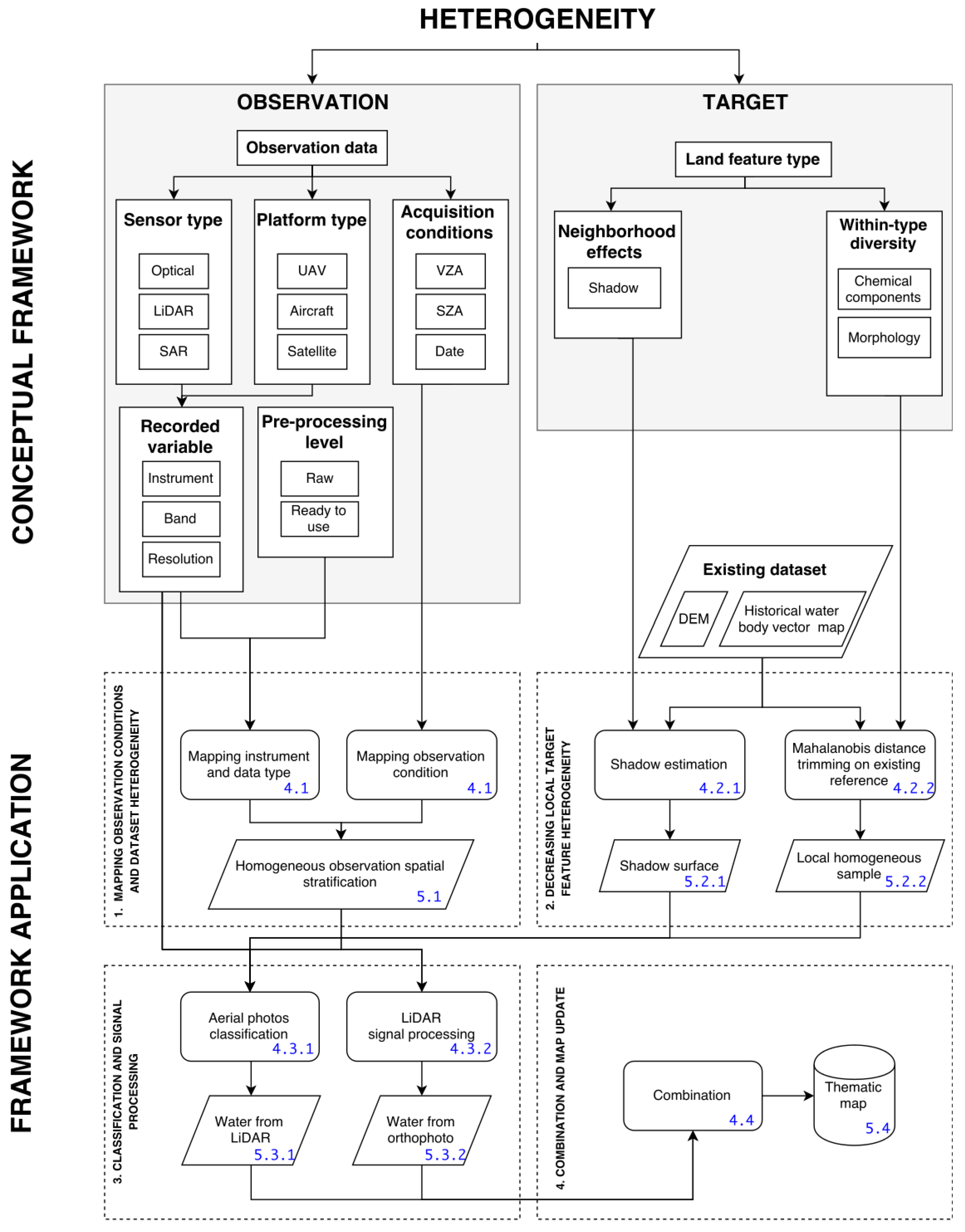
2. Conceptual Framework

The framework rationale is based on the idea of reducing the heterogeneity of both observations and target land features. The underlying assumption is that feature detection is improved by reducing observational and target heterogeneity. First, observational heterogeneity depends on the platform used (UAV, airborne, satellite), the sensor type (optical, LiDAR, SAR), the pre-processing level and the recorded variables (instrument model, spectral band, resolution) (Figure 1 upper left). Additionally, observational heterogeneity depends on the acquisition conditions such as the season and time of the day characterized by the View Zenithal Angle (VZA), the Sun Zenithal Angle (SZA) and the date. Second, the target landscape feature itself is also heterogeneous by nature (Figure 1, top right). Specifically, the target features have a within-type diversity defined as the specific spectral heterogeneity of a given water body compared to other water bodies and is determined by the water components (chemical, organic) and the water body morphology (water depth, sediment type). It is independent of its observation and its neighborhood. In addition, the target features are affected by the neighborhood effects which consist in the effects altering water reflectance caused by local features such as shadows coming from bridges, trees, and buildings.

The framework proposed in this paper is applied to update a pre-existing historical water body vector map (Figure 1, lower half). First, the mapping of the instrument and data type along with the observation conditions provides a stratification used to split the data into homogeneous sets to process. In a second step, the proposed framework addresses the heterogeneity of the targeted feature itself and reduces local heterogeneity by mapping the neighborhood effects of shadows on water. A third step consists in a multi-source classification that handles the within-type diversity of the targeted landscape features; this results in water maps from aerial photos and LiDAR. Those two results are finally combined in a fourth step to update the pre-existing water map.

3. Study Area

This section describes the study area with a focus on water bodies’ heterogeneity and illustrates the heterogeneity of the target feature (Figure 1, upper right). Additionally, the historical water body vector map to update is detailed.

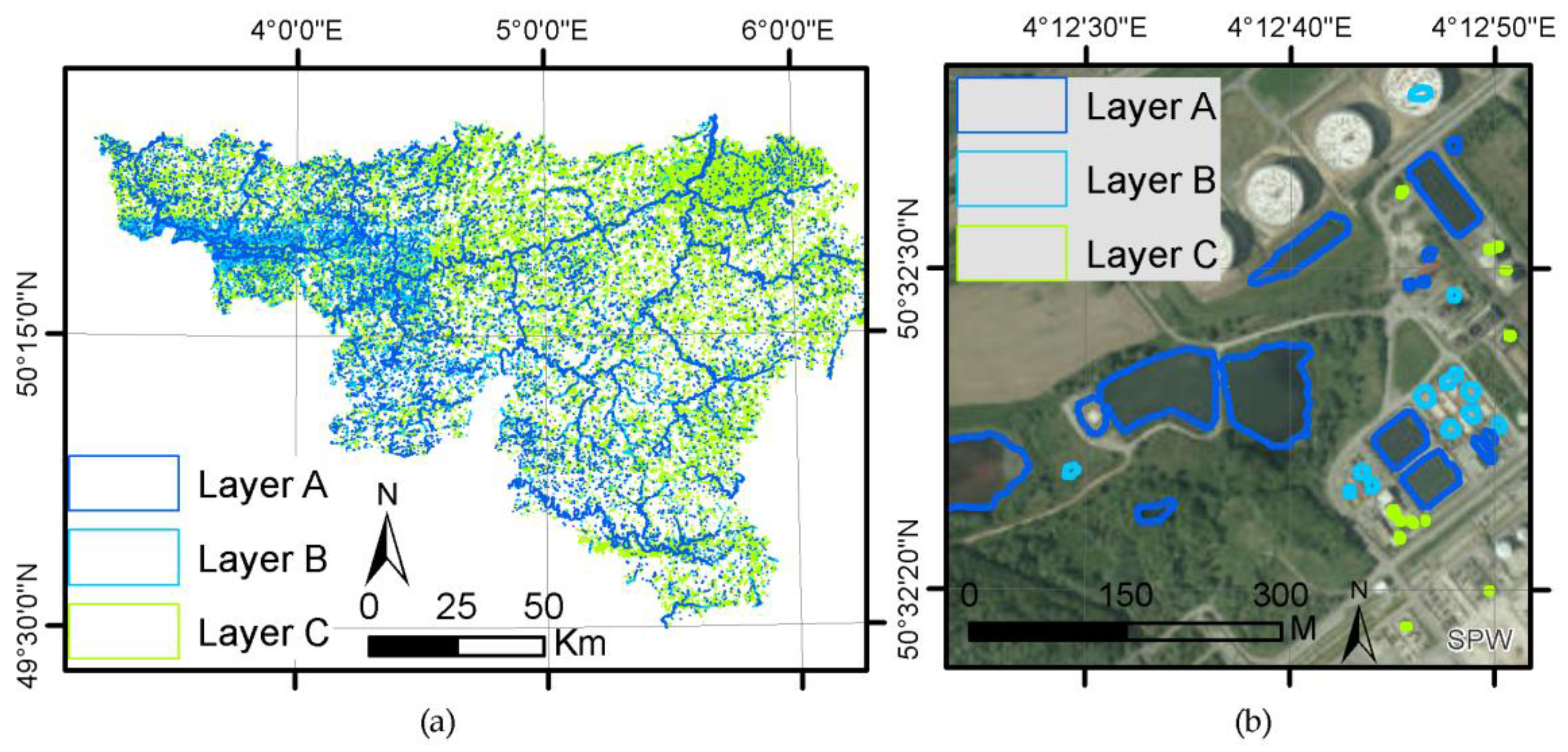
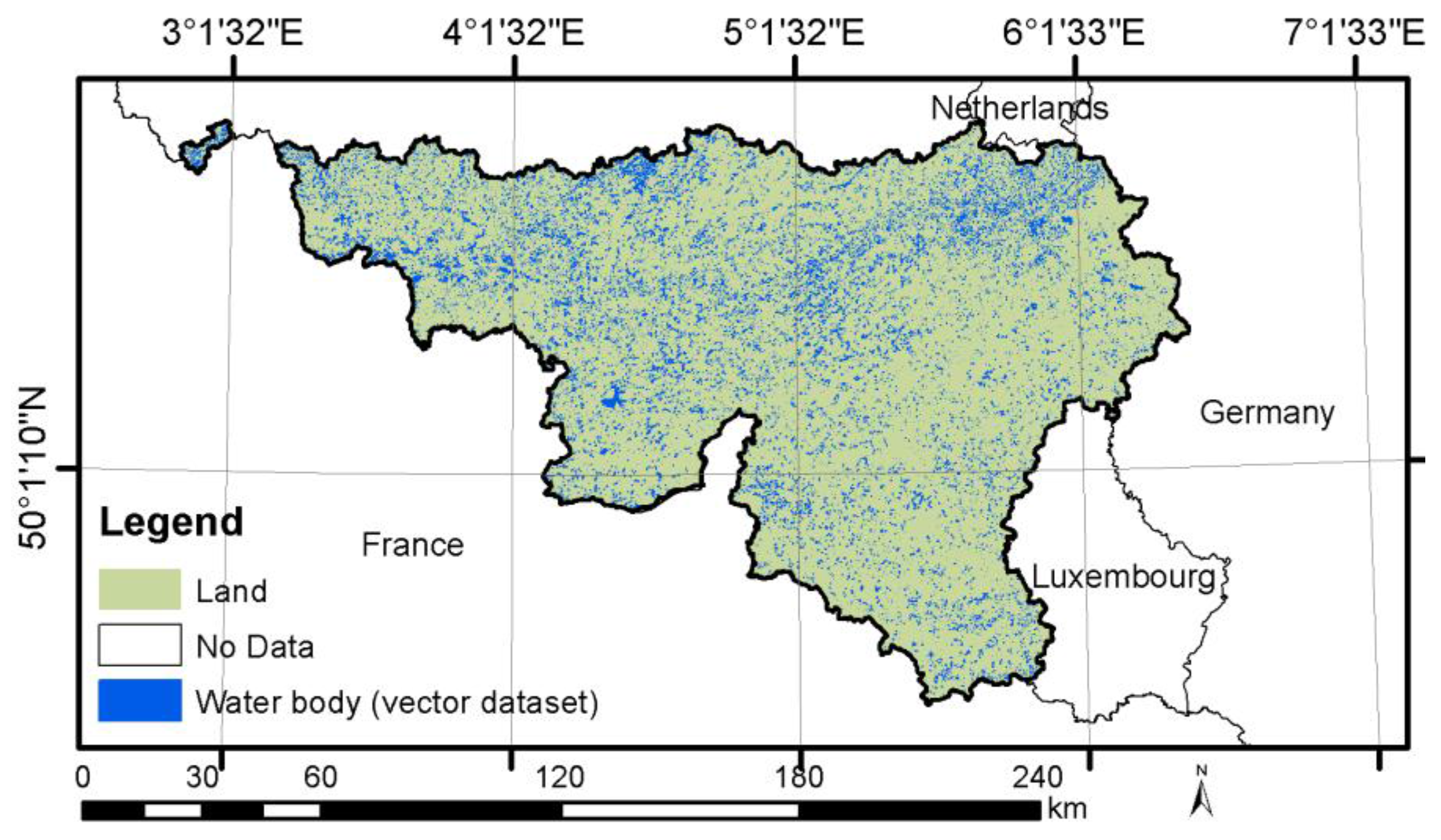
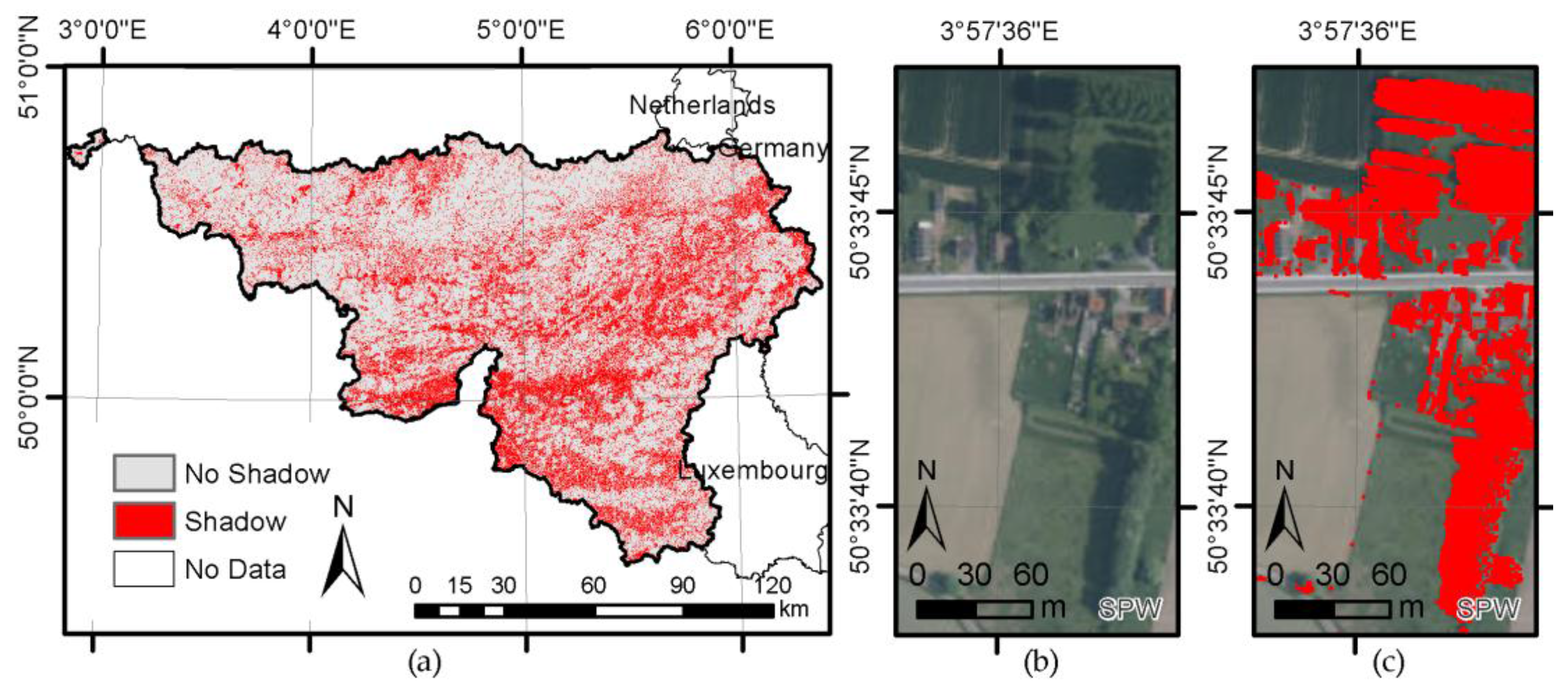
3.1. Study Region

The Walloon Region (Wallonia) forms the southern part of Belgium and covers about 17,000 km² (55% of Belgium). Altitude ranges from 25 m to 694 m. The Walloon Region has a climate influenced by the Gulf Stream and ocean disturbances. The weather is characterized by moderate temperatures, high cloudiness, and frequent but sparse rainfall. It rains on between 160 and 200 days per year in Wallonia, for a mean annual precipitation ranging from 700 mm to 1400 mm, representing a water intake of about 15–16 billion cubic meters per year.

A water body is defined as a natural or artificial depression filled with water continuously or intermittently. The variety of uses, the morphology, and the composition of water bodies are linked to human activities and history. Rivers and streams are categorized into navigable or non-navigable and may have a natural or an anthropogenic origin. There are about 12,000 rivers located on four major river watersheds. The total surface of water bodies is 0.7% of the land surface. Apart from anthropic reservoirs and hydraulic power plant dams, there is no large lake in Wallonia. Ponds are frequently found and most of them have an anthropic origin. Ponds were created in arable land to water livestock (Figure 2a), to raise ducks and geese, for flax and hemp retting, to nurture fish and frogs, for watercress, and for game hunting. Ponds were also unwittingly created due to mineral extraction (Figure 2b) [47]. There are also many ponds that have been created for biodiversity conservation, water management, and flood risk management (Figure 2c–g). Recently, financial incentives from the European Common Agricultural Policy (CAP) have been given to farmers to preserve the small ponds in arable land [48]. Some ponds may also have a natural origin (Figure 2h). In particular, there are natural water bodies as a result of the water network evolution in floodplains such as backwaters. Some ponds in peat bogs—the ‘lithalse’ or the ‘palse’—have an Ice Age origin. Others, the ‘mardelles’, are formed by dissolution of the limestone in the marl. Due to their origin and their use, the water bodies thus have a large morphological and compositional heterogeneity. This heterogeneity in water bodies means that any successful mapping technique needs to be able to take into account all of these conditions.

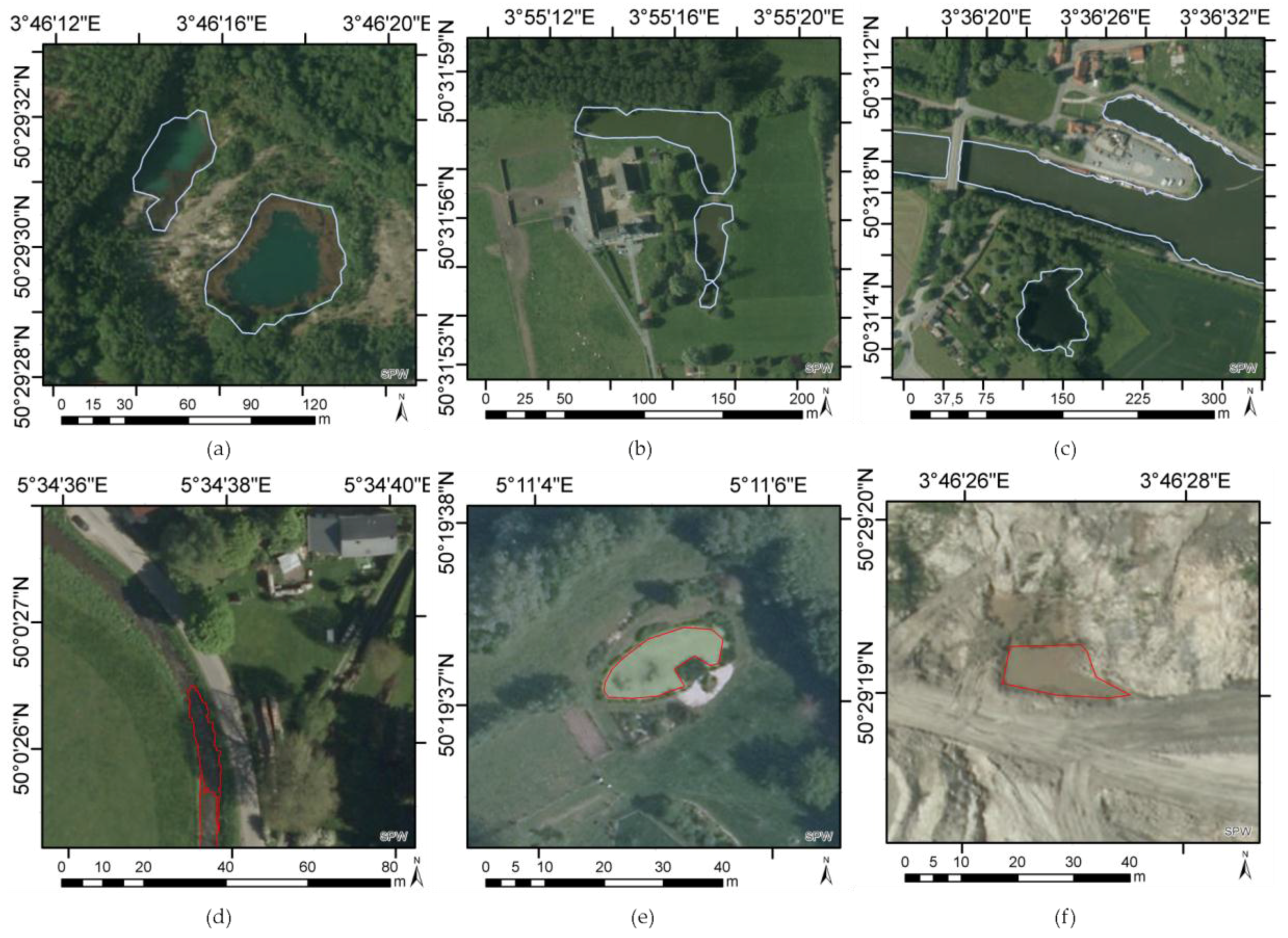
3.2. Historical Water Body Vector Map

The proposed framework is applied on an outdated water body dataset (Figure 3) created in 2005. This database contains water bodies excluding rivers and is the result of the merging of various databases [49]. The vector database [50] contains 36,335 water bodies with a geometric accuracy ranging from 0.25 to 1 m. Since 2005, the database has been updated by visual interpretation of aerial photos: in 2006–2007 (1% of the features updated), 2009–2010 (6% of the features updated), and 2012–2013 (1% of the features updated). Due to resource limitations, the update cannot cover the whole extent, resulting in only a partially updated dataset. Moreover, the operator focuses on updating water body delineation but not on adding new water bodies, resulting in an incomplete dataset.

4. Framework Application

The conceptual framework is applied in a four-step workflow (Section 4.1, Section 4.2, Section 4.3 and Section 4.4) described at the bottom of Figure 1. The first step (Section 4.1) uses metadata about the different data acquisitions to separate the products into groupings with consistent characteristics. The observation conditions mapping of the aerial photos and the LiDAR results in spatial stratification with homogeneous set of data. The second step (Section 4.2) uses the pre-existing historical water body vector map to produce labeling data from which the outliers are removed through an iterative trimming of the data. Aerial photos are then cleaned by removing shadows via shadow projection estimation. The third step (Section 4.3) consists in aerial photo classification dealing with the water body within-type diversity and LiDAR signal processing handling the data sources specificities. The last step (Section 4.4) of the workflow combines the results to update the initial dataset. Finally, the last section (Section 4.5), not represented in Figure 1, presents the validation methodology.

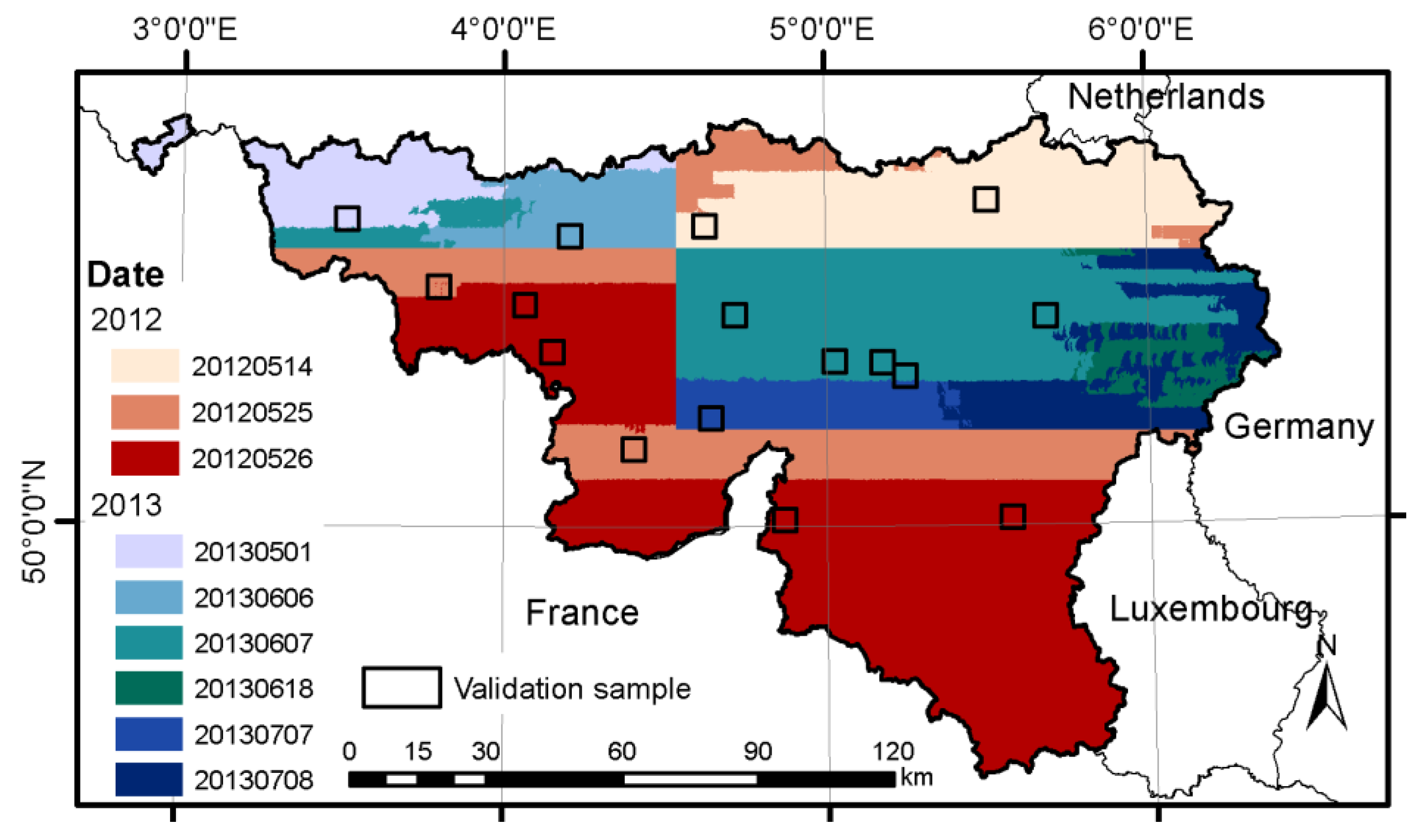
4.1. Mapping Observation Conditions and Dataset Heterogeneity

Because the quality of the observations varies so much as a function of instruments and other characteristics not related to the target land feature, aerial photos classification and LiDAR signal processing were applied separately by tuning the methods for each set of data sharing acquisition characteristics. First, the aerial photos are split according to the cameras used, the date of the acquisition and the hours of acquisition used as a proxy of the SZA. Second, the LiDAR dataset is split according to the instrument and the date of acquisition. This produces a homogeneous observation spatial stratification (Figure 1, lower half, box 1), with different strata then processed separately.

4.1.1. Aerial Photos

The aerial photos were taken on nine separate days for 2012–2013 (Figure 4a) using three UltraCam cameras (Figure 4b) with four channels: red, green, blue, and near infrared. The acquisition time varied from 7 a.m. to 3 p.m. (Figure 4c) and the vertical sun angle varied from 34.2° to 63.2° (Figure 4d). The flying altitude ranged from 4181 to 4617 m. The images were first radiometrically corrected. Automatic homologous points were generated and the Bundle Adjustment algorithm [51] was used to correct the distortion and to obtain an orthophoto mosaic. Verification acceptance provides a maximum RMSE of 0.856 m in X and 0.861 m in Y for 2012, and 0.977 m in X, and 0.71 m in Y for 2013 [52].

The result is an aerial orthophoto mosaic composed of 5872 irregularly shaped tiles (Figure 4e). The image has a Ground Sampling Distance (GSD) of 25 cm and is 1,012,021 pixels in X and 586,567 pixels in Y, thus totaling 593 billion of pixels. To give some idea of comparative orders of magnitude, the conterminous U.S. Landsat WELD mosaic [53] corresponding to 459 Landsat scenes contains in total 11 billion pixels. Consequently, the orthophoto data volume of the current study corresponds to the equivalent of more than 50 conterminous U.S. Landsat mosaics in terms of pixels. In other words, in one 30-m Landsat pixel, there are 14,400 25-cm pixels. For processing and storage, the image is stored as a virtual GDAL dataset (VRT) [54].

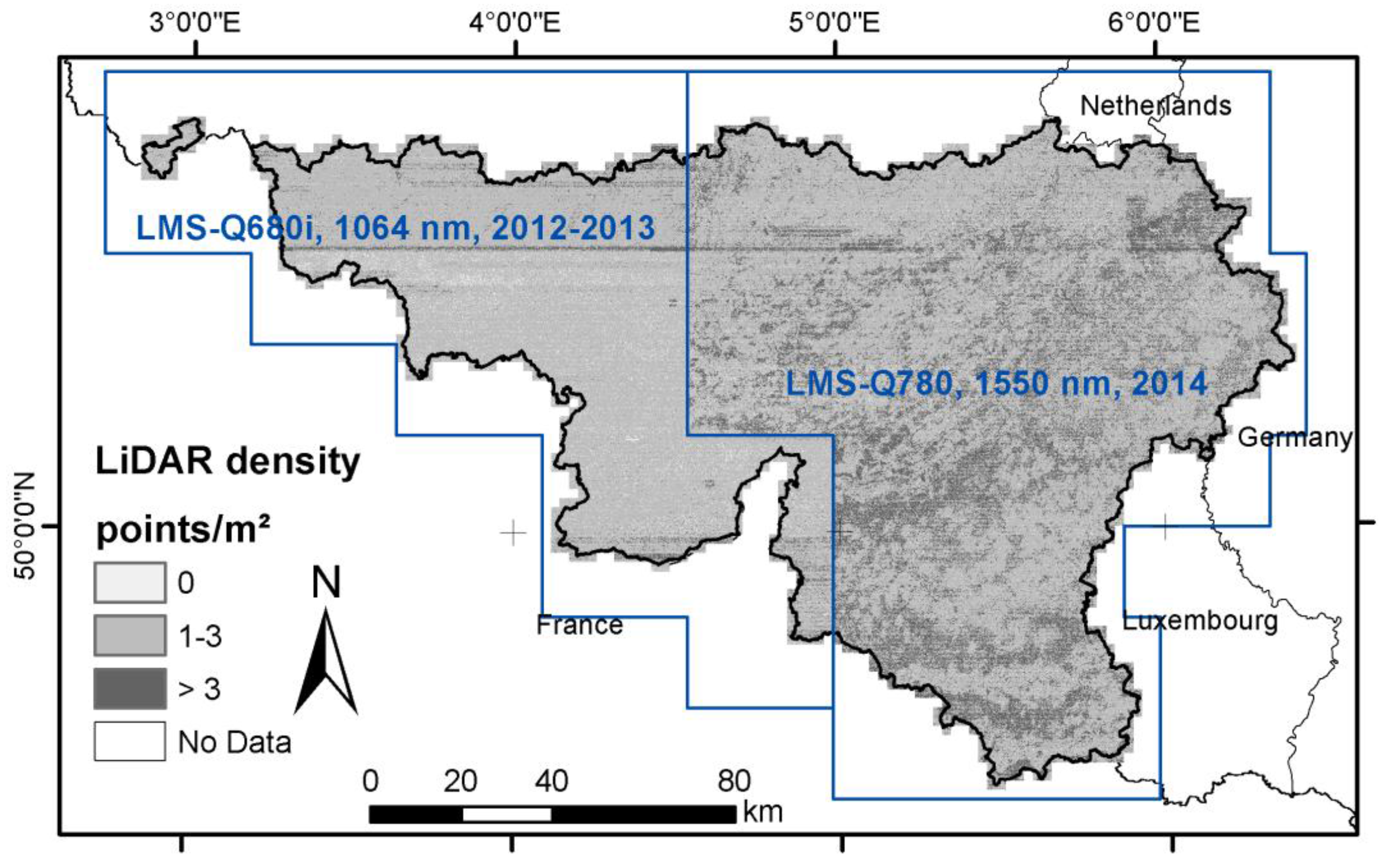
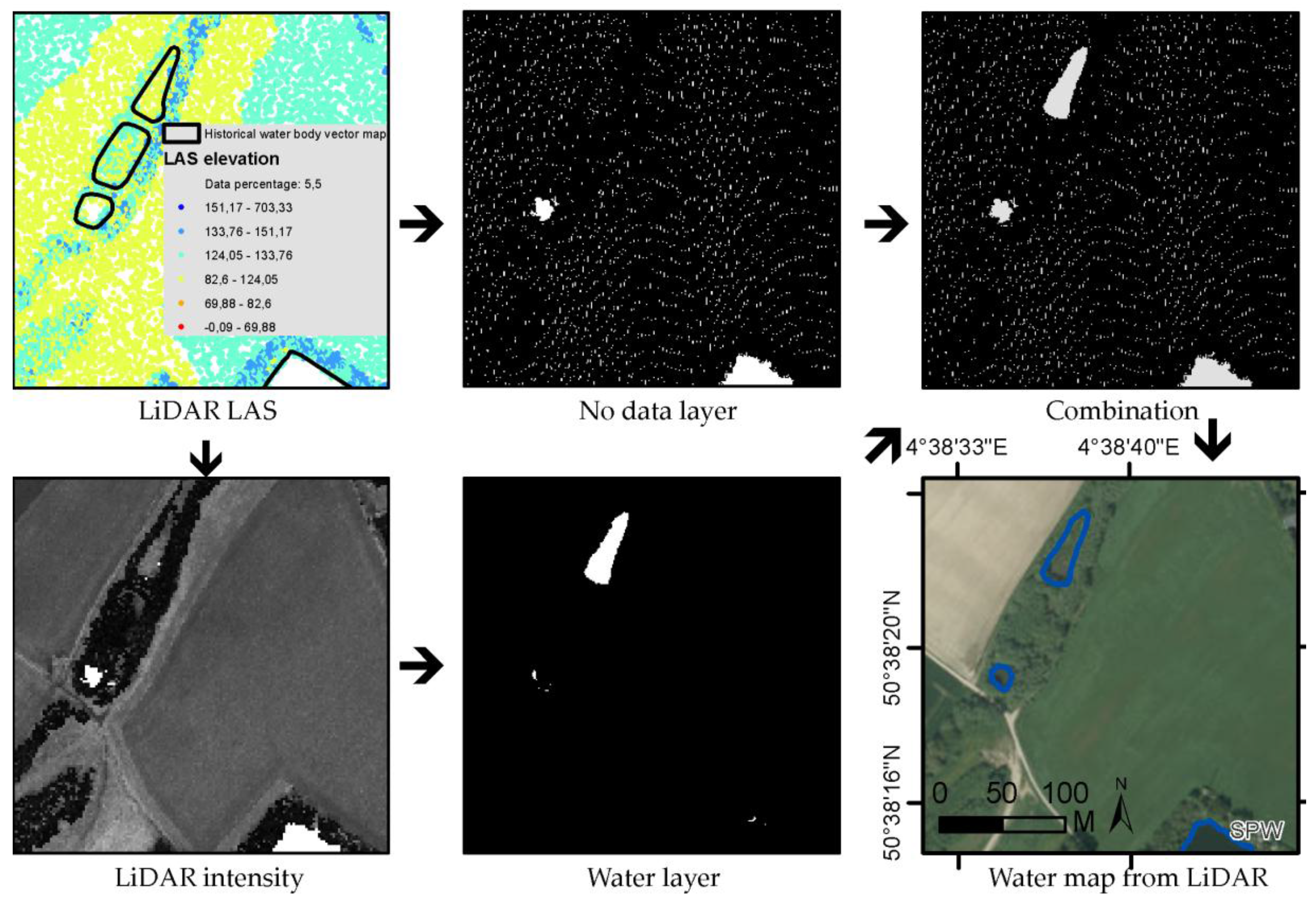
4.1.2. LiDAR

The LiDAR acquisitions completed from 2012 to 2014 used two different sensors depending on the year of survey (Figure 5): Riegl LMS-Q680i for the western part in 2012–2013 and Riegl LMS-Q780 for the eastern part acquired in 2014. The power and wavelength are different for these two devices, the first one having less power, fewer echoes, and a less suitable wavelength (1064 nm) than the second (1550 nm). Those two spatial strata will therefore be processed separately. The mean pulse density over the whole region is about 1.51 pulse/m². The western part was acquired with a lower density than the eastern part (Figure 5), which could affect the water detection, especially in vegetated areas where the pulse may not reach the soil. The required acquisition period was from January to March to limit the foliage effect in order to generate a Digital Terrain Model (DTM). The total of surveying days over the two years is 36 but the time slot was larger than expected, ranging from December to April. The altitude of acquisitions ranges from 1015 m to 1550 m above ground level. The swath is about 1700 m. Comparison of the DTM generated from LiDAR with reference topographic points reveals a maximum RMSE in Z of 0.25 m.

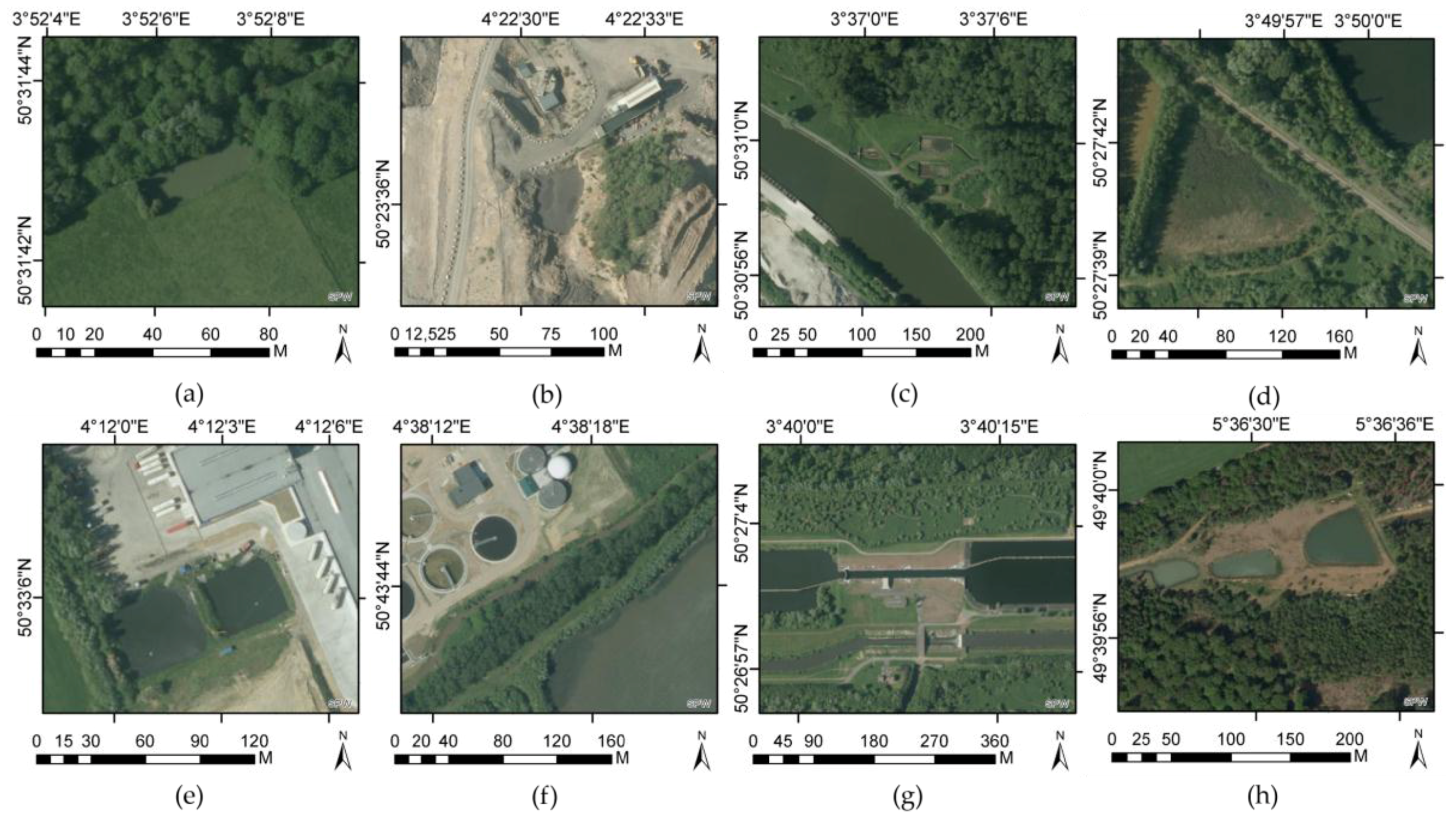
4.2. Decreasing Local Target Feature Heterogeneity

The local heterogeneity on the aerial photos was addressed by two methods (Figure 1, lower half, box 2). First, shadows were modeled using a Digital Surface Model (DSM) and the sun angle associated with each aerial photos; Section 4.2.1 describes how these estimates are used to remove shaded pixels from the water body delineations. After confirming the presence of a water body on the historical water body vector map, each water body was sampled. From this sample, the shaded points were removed along with outliers by means of an iterative trimming (described in Section 4.2.2).

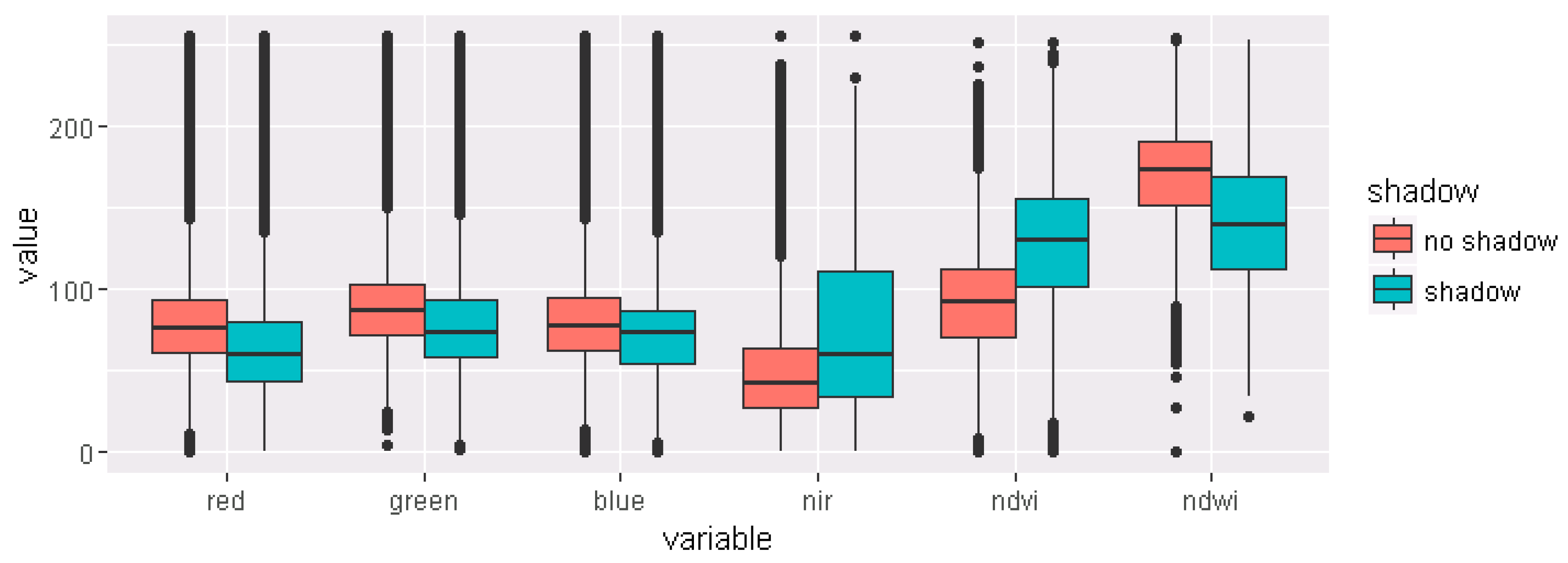
4.2.1. Neighborhood Effects: Shadow Estimation

Xie et al. (2016) indicate that no existing water index can extract water information while at the same time suppressing the false alarm of shadow. Indeed, benchmarking reveals that the shadow seen in the aerial photos was frequently misclassified as water. This was particularly true in this study as the contrast in the low reflectance values was poor and as the sun vertical angle was frequently close to 30°, resulting in frequent large shadows.

To tackle this shadow problem, geometric shadow estimation is proposed. The approach proposed consists of shadow modeling using information on the sensor, light source, and geometry of observed objects. This approach determines the location of shadows precisely but the geometry of the scene and light sources must be known, which could be restrictive [55]. In the same way as proposed here, other studies have used laser data to model shadows over high-resolution remote sensing imagery [56,57,58]. In this study, first the azimuth and vertical sun angle were calculated using the acquisition time of the photos. Second, a DSM along with the sun angle makes it possible to predict the geometric projection of the shadow. The sun elevation and azimuthal angle were calculated from the time and the position of the aircraft during the acquisitions for the 5872 tiles. The 1-m resolution DSM was derived from the first-return LiDAR data. The tangent of the sun elevation angle corresponds to the ratio of the object height on the shadow projection, allowing for estimation of the shadow. The algorithm produces a shadow mask.

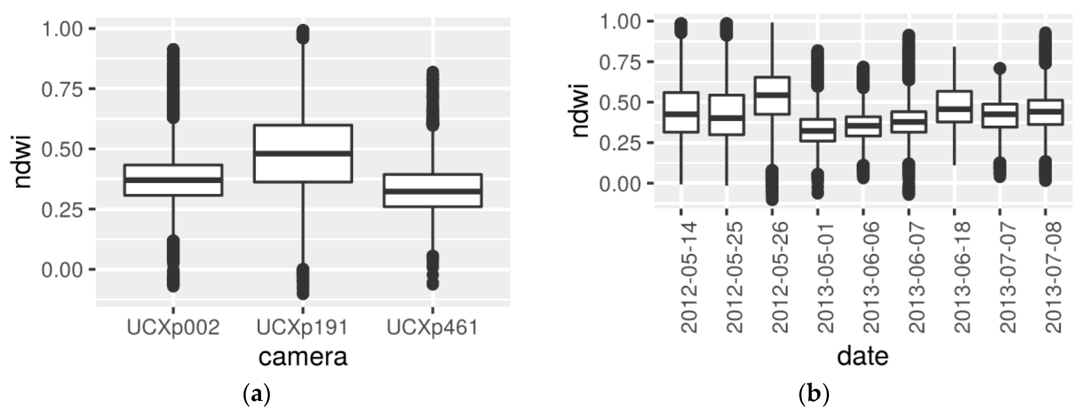
4.2.2. Within-Type Diversity

The within-type diversity of water bodies is caused by the chemical component of water and by the sediment of the above surface and may result in very different spectral signatures of water, as illustrated in Figure 2. The approach proposed to handle this within-type diversity over aerial photos is to use an unsupervised classification with a large number of clusters and then to label the clusters with the highest probability of being water according to a cleaned sampling of the historical water body vector map. The rationale behind this is that using a large number of clusters makes it possible to capture the different water classes and to separate them efficiently. In the subsequent aerial photo unsupervised classification (Section 4.3.1), a representative sampling of points that reliably lie within actual water body boundaries is needed to label the different water classes. This section describes the three steps required to obtain these points. After a confirmation of the water presence using a water index over the historical water body vector map, a sampling of points is drawn and then cleaned to keep only those points not affected by surrounding elements.

As the historical water body vector map is not up to date, it may contain disappeared water bodies; a pre-confirmation using the Normalized Difference Water Index (NDWI) makes it possible to remove dry water bodies. The NDWI from McFeeters [59] used a normalized difference between green and near infrared (NIR) bands resulting in a value for each pixel ranging from −1 to 1 (Equation (1)):

$$\mathrm{NDWI}=\frac{\mathrm{GREEN}-\mathrm{NIR}}{\mathrm{GREEN}+\mathrm{NIR}}$$

(1)

Defining the NDWI threshold best suited to separate water from land is challenging over large areas as it is known to be valid only locally. Therefore, a method to automatically retrieve the status of the water body was designed. The NDWI thresholds (from −1 to 1 with a 0.01 step) were systematically assessed to separate water from land. The threshold maximizing the number of confirmed water bodies was selected, allowing the removal of disappeared water bodies from the historical water body vector map.

A sampling consisting of 200 random points in each water body with a 1-m minimum allowed distance was drawn with the Create Random Points tool form ArcGIS [60]. The number of 200 was selected in order to characterize the within-type diversity of the water reflectance. The points fallen in shadow (retrieved in Section 4.2.1) are removed. All the points with a Normalized Difference Vegetation Index (NDVI) [61] value greater than 0.2 and a near infrared value greater than 180 (on a 256-value scale) are also removed as those values are unrealistic for water surfaces.

Thirdly, for each sampled water body with at least 50 points, the Mahalanobis distance [62] is calculated. The Mahalanobis distance is a measure of the distance between a point and a distribution. It is a multi-dimensional generalization of the idea of measuring how many standard deviations away is from the mean of a distribution. The Mahalanobis distance is unitless and scale-invariant, and takes into account the correlations of the dataset. The distance between each point and the mean of the value in the six bands of the water body considered (red, green, blue, near infrared, NDVI, NDWI) is calculated with Equation (2) described by [63]:

$$D_i=\sqrt{{\left(x-m_i\right)}^T{\mathsf{\Sigma }}_i^{-1}\left(x-m_i\right)},$$

(2)

where D = Mahalanobis distance, i = the i class, x = data with n dimension (where n is here equal to 6 for red, green, blue, near infrared, NDVI, NDWI), ${\mathsf{\Sigma }}_i^{-1}$= the inverse of covariance matrix, and $m_i$ = the mean vector of a class. An iterative trimming as already used by [64,65,66] is applied until all the points are in the confidence interval of a Chi-Square law of 95%. The points distant to more than 95% of the distribution are removed. A new mean with the remaining points is then calculated along with their Mahalanobis distance to the mean. This filtering allows removal outliers and points affected by the local context while taking into account the water spectral within-type diversity. The result is a sample of points located on confirmed water bodies for each stratum that will be used in the next section to label the clusters.

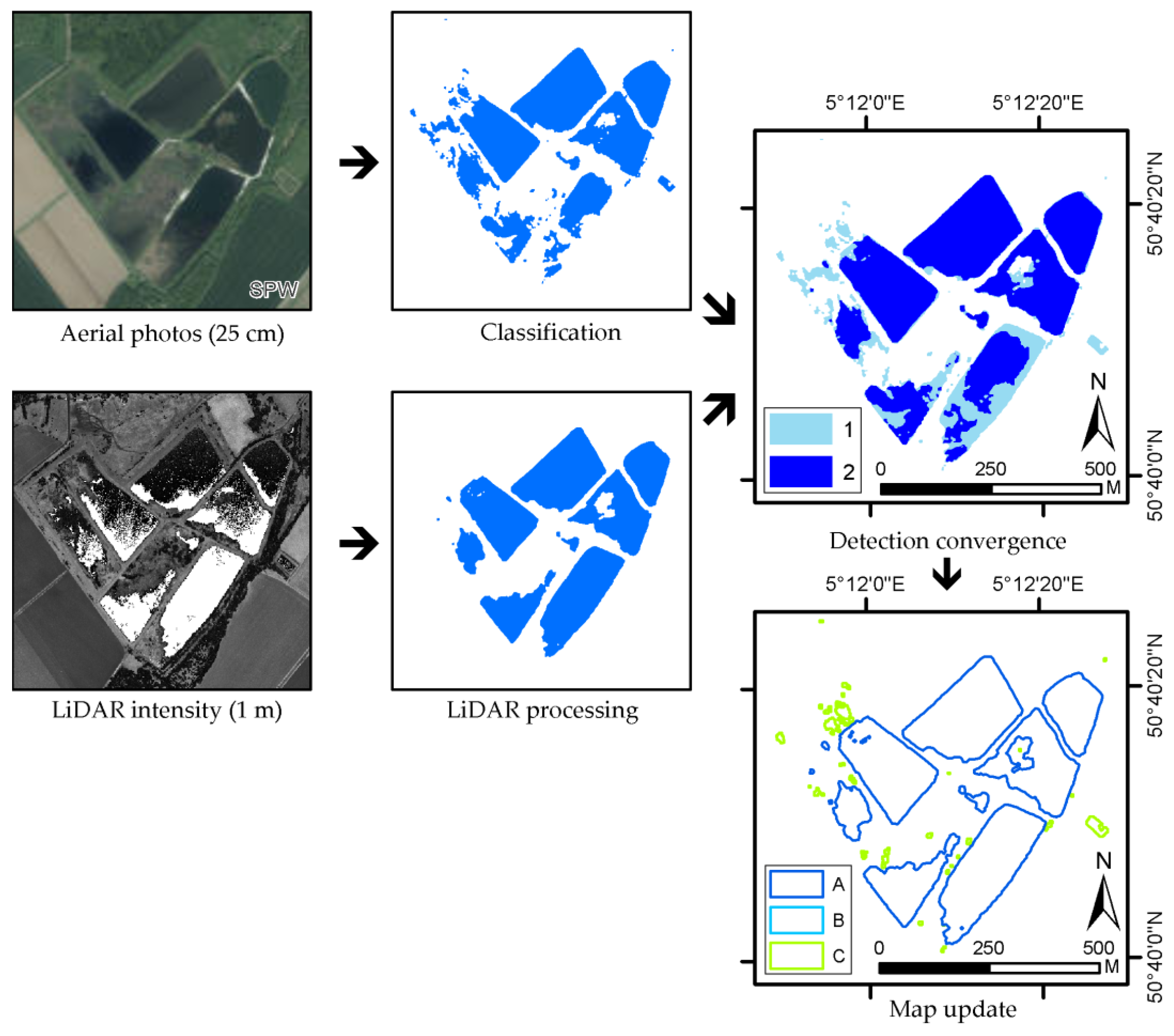
4.3. Classification and Signal Processing

The two different sources (aerial photos and LiDAR) are handled separately (Figure 1, lower half, box 3). Section 4.3.1 describes the aerial photos classification, labeling, and post-processing for which the previously presented samples retrieved from the cleaning of an existing vector dataset are used as labeling. The labeling corresponds to the assignment of a land cover class to a cluster resulting from the unsupervised classification. Section 4.3.2 describes how LiDAR is handled to retrieve surface water.

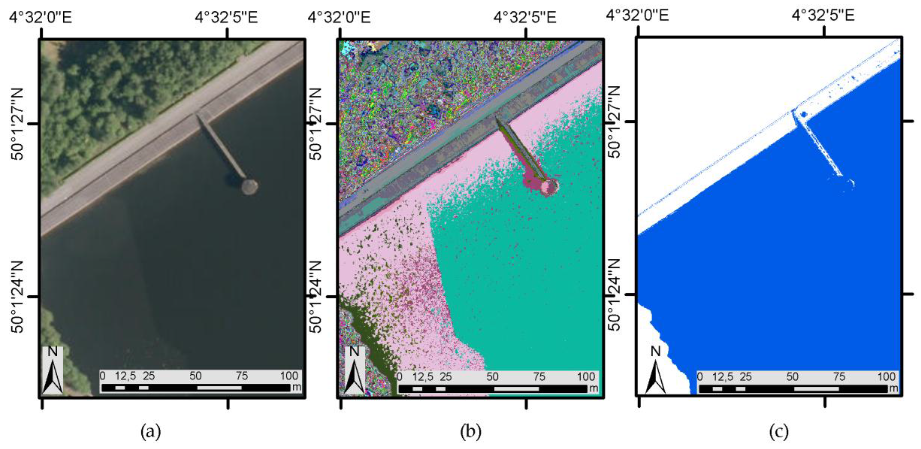
4.3.1. Aerial Photo Classification

For each grouping of aerial photo acquisition (defined as stratum in the Section 3), aerial photos are classified into a large number of clusters. In addition to using the red, green, blue, and near-infrared bands of the imagery, the classification used NDWI and NDVI as providing valuable information regarding vegetation and water.

An unsupervised K-means clustering is applied on each stratum independently over the six-band file: red, green, blue, near-infrared, NDVI, NDWI. The per-stratum number of clusters, which will be used to generate class membership, was set to 500. This arbitrarily large number of clusters was deemed to be large enough to separate the large heterogeneity of the land surface into different clusters. This helps separate water from non-water surfaces, as well as separate visually different types of water bodies. The training set size is 50,000 pixels and the maximum number of iterations for the learning step used is 10,000. The classification was done using Orfeo ToolBox (OTB) on a supercomputing facility. OTB [67] is an open-source C++ library for remote sensing images processing initiated and funded by CNES (French space agency) and enabling state-of-the-art processing of large images.

For each of the 36 stratum, the frequency of clusters corresponding to water in the cleaned sampled points of the historical water body vector map obtained at the Section 4.2 is then computed. This permits to label the corresponding clusters as water or land.

A number of post-processing steps then permits the reduction of artifacts and commission errors. First, the shadow (retrieved at Section 4.2.1) and buildings from ancillary data are removed. Second, a sequence of mathematical morphology operations realized with the Binary Morphological Operation algorithm from OTB [67] is applied: erode (1 m), dilate (3 m), erode (3 m), and dilate (1 m). The aim of those operations is to preserve edges and shapes as much as possible while removing artifacts. These morphology operations are generic tools widely used in the image-processing community. In this study, the first 1-m erosion removes lonely pixels while the closing operation (3-m dilate followed by 3-m erode) makes it possible to fill the gaps on water bodies. Finally, the last 1-m dilate counterbalances the first erode operation. Those filters thus have a positive effect on the results by removing lonely pixel artifacts and by filling gaps in the water bodies. However, the morphological operations have a negative effect on the results by removing every lonely pixel (water bodies of 1 x 1 m are lost) and by filling 3 × 3 m gaps that are not gaps (islands smaller than 9 m²).

Finally, a raster mosaic is built with all the strata using GDAL [54] and is then converted without simplification into vector data in order to update the existing vector dataset.

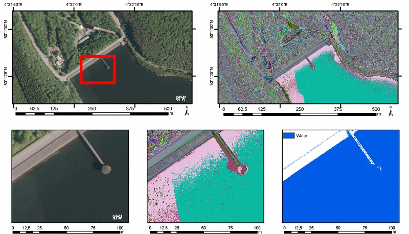
4.3.2. LiDAR Signal Processing

Next, the framework derives an alternate set of water body delineations using an entirely different source of data, LiDAR. The LiDAR signal is most of the time either fully absorbed by the water surface or lightly reflected with Lambertian reflection. The potential presence of water is thus indicated by a low return intensity or by the absence of return. A caveat when using LiDAR to detect water is that other surfaces such as dark roofs (shingle or roofing) also absorb the LiDAR beam. Additionally, forests with heterogeneous canopy height trap the beam returns. Vegetated part of wetlands and roads can also absorb most of the signal and thus are frequently confused with water. Moreover, the LiDAR returns over water could be specular. The return intensity may be at its maximum when the beam is reflected specularly over water, improving the omission of water bodies.

In the current study, the LiDAR data were processed separately for the eastern and western strata (Figure 5). For each stratum, the LAS (LASer file format exchange) data are extracted as two different rasters. (1) First, the LAS layer was converted to raster selecting the cells designated as water by the pre-classified water to a 1-m raster water layer raster using a Binning Maximum Simple interpolation (algorithm from [60]). This flag is obtained by thresholding small intensity values of the last echo of the LiDAR pulse. The thresholds were defined by extracting the frequency histograms of the intensity to split visually the intensity values between water and no-water. The threshold varies according to stratum as the power of the LiDAR used differs. (2) Second, the LiDAR intensity was also extracted using the Binning Maximum None interpolation (algorithm from [60]) into a 1-m resolution raster to retrieve a no data layer indicating the location where the pulse was fully absorbed. This second layer is highly contaminated but contains a lot of water bodies not present in the first layer. These two layers are then combined and most of the artifacts are removed with a morphological mathematics operation realized with the Binary Morphological Operation algorithm from OTB [67] with the following sequence:

• Binary union of the water layer and the no data layer is eroded (3 m), and dilated (3 m). This removes most of the artifacts but will remove small water bodies.
• A recombination of the resulting layer with the water layer allows recovery of small water bodies lost in the previous steps. The resulting layer is then dilated (2 m), eroded (3 m) and finally dilated (1 m).
• This sequence is followed by the removal of the remaining buildings using ancillary data [68]. As the building ancillary data are not up to date, some buildings may remain.

The resulting raster is then transformed into a vector.

4.4. Combination and Map Update

Because the two new maps of water bodies have some degree of disagreement, they are blended using the following workflow illustrated in Figure 6 (general outline, see Figure 1 lower half, box 4). If a water body is detected on both aerial photo classification and LiDAR, the confidence of having a water body is higher. LiDAR-detected water bodies have more accurate edge as the pulse may go through the canopy to reach the water. The geometrical union of the aerial photo classification layer and the LiDAR layer gives a convergence of the detections by summing the occurrence (detection occurrence number: 0, 1, 2). The layers are then combined to prioritize the update in three successive layers (A, B, C) facilitating the update while taking the best contours as described in Figure 6. The Layer A contains the water bodies detected by both the LiDAR and aerial photos with the contour of the LiDAR. Layer B contains the remaining polygons detected by LiDAR only. Layer C contains the remaining polygons detected by the aerial photo classification.

4.5. Validation

4.5.1. Validation Dataset

After the merging of the dataset in Section 4.4, the results are evaluated. The validation dataset is based on a random sampling of the aerial photo acquisitions stratified in the years (Figure 7). In total, 16 zones of 5 × 5 km were used (eight for 2012 and eight for 2013). In those extracts, the water bodies and their extents were manually delineated by two operators and are considered as ground truth. The area sampled represents 2.5% of the total area and contains 1334 water bodies, of which 245 are new (absent from the historical water body vector map). The validation is based on visual interpretation and includes all the water surfaces.

4.5.2. Quality Indices

The quality evaluation relies on the detection efficiency and the detection cost. These indices were defined as they were relevant in the applied case presented in the study where the classical user and producer accuracy are not suited. The detection efficiency is described in Equation (3):

$$DetectionEfficiency=\frac{N_{detected}}{N_{real}},$$

(3)

where $N_{detected}$ corresponds to the number of water bodies detected and $N_{real}$ corresponds to the number of water bodies in the validation. This gives information about the omissions of the resulting map.

The detection cost is described in Equation (4):

$$DetectionCost=\frac{N_{toreview}}{N_{real}}$$

(4)

where $N_{toreview}$ corresponds to the number of polygons to be reviewed by the operator. This number corresponds to all the polygons of potential water detected by the framework, including wrongly detected water bodies. The detection cost gives quantitative information about the work required for an operator to review the map obtained by the framework and gives information about the commission error.

Those two evaluations are calculated on Layer A, B, C, and on the total layer for different area groups of water bodies: 25–50 m², 50–100 m², >100 m², and all sizes together.

5. Results

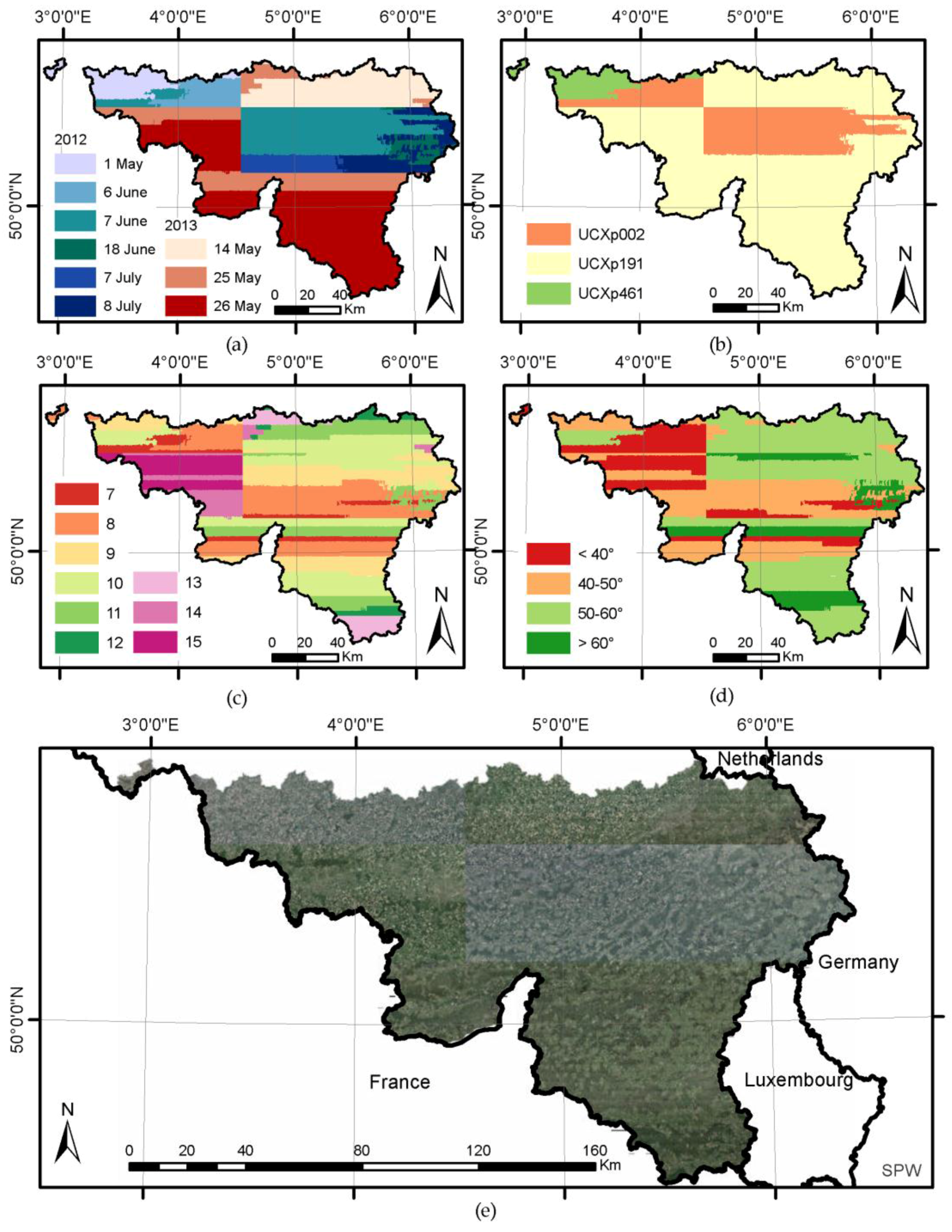
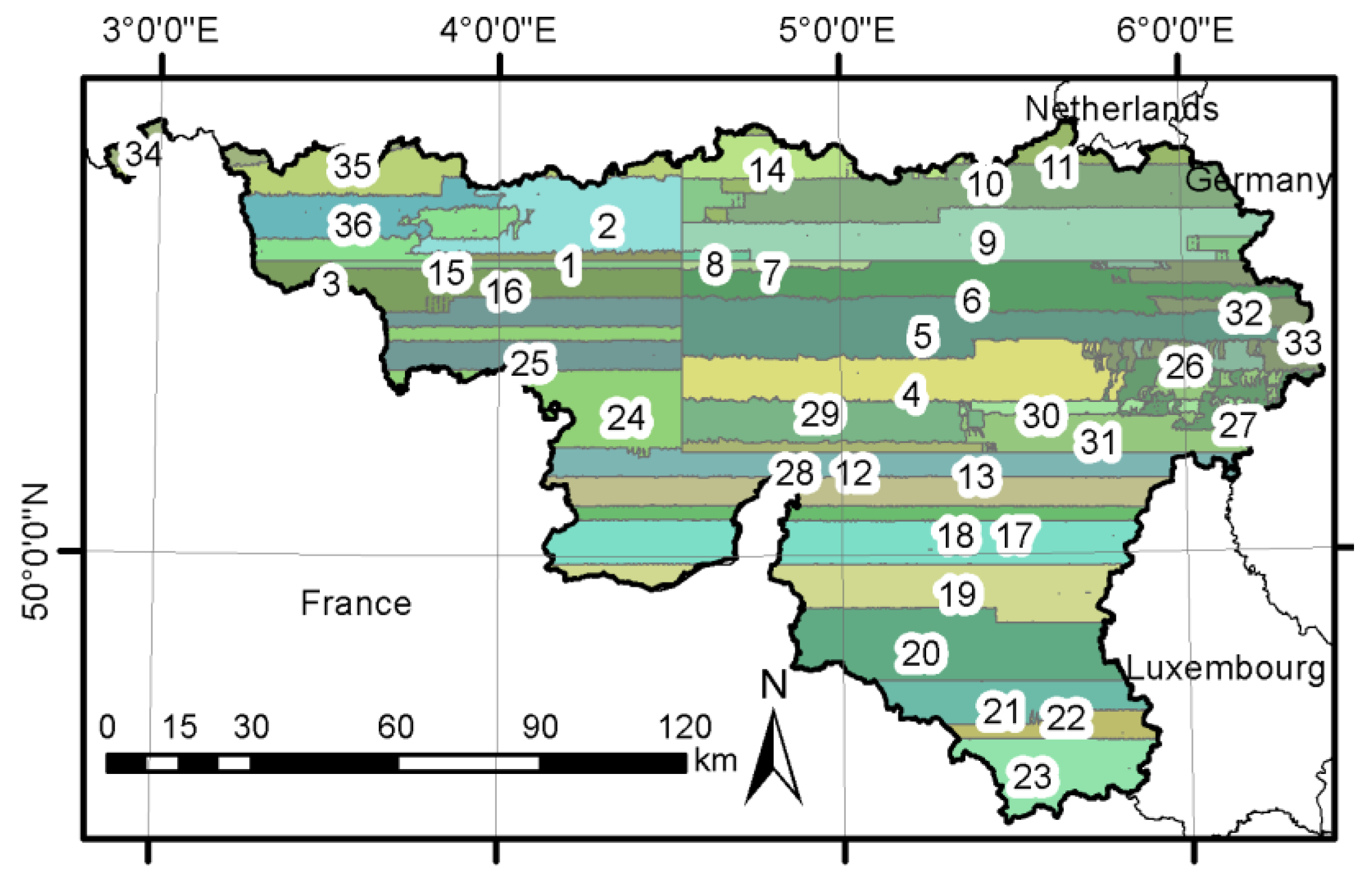
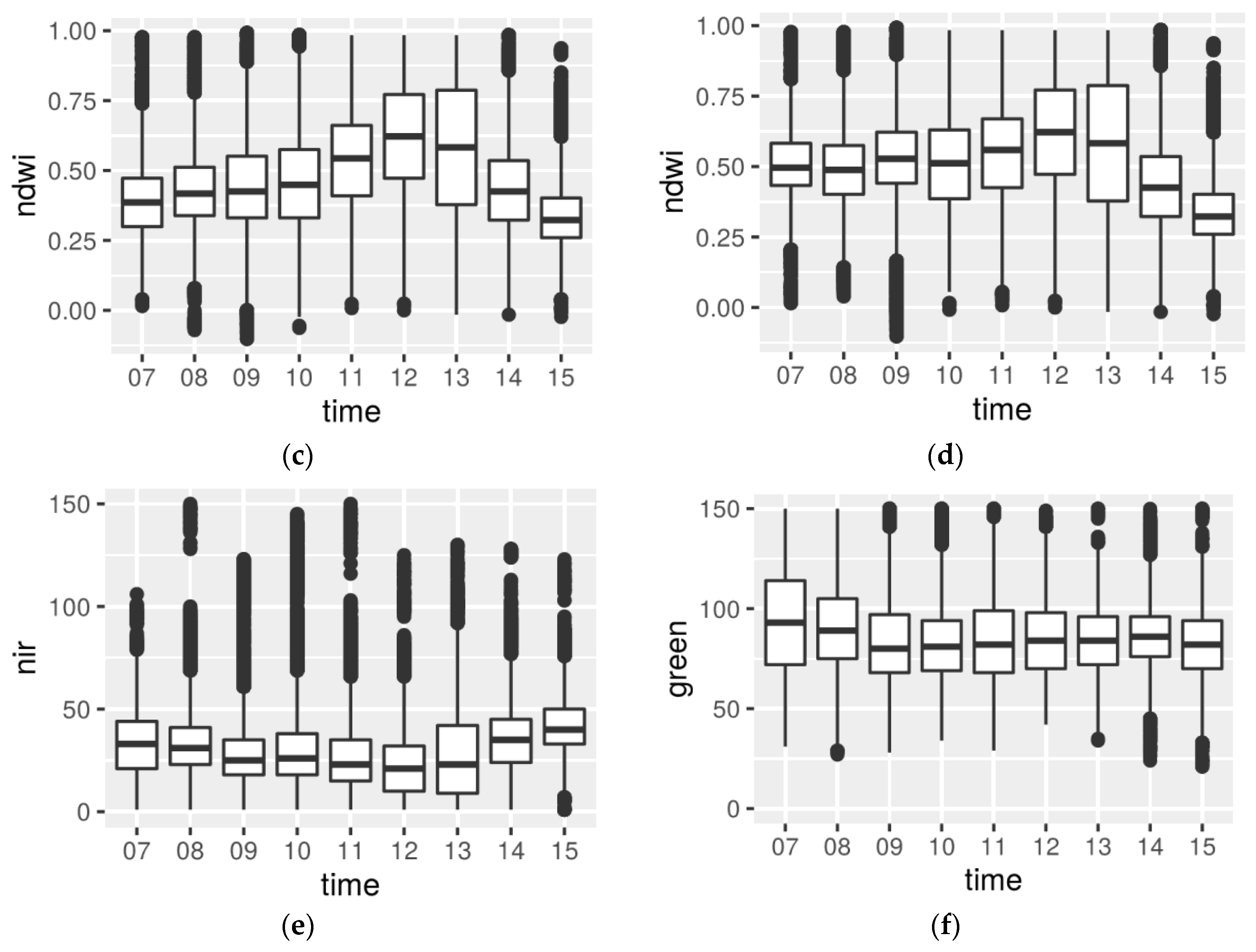
5.1. Mapping Observation Conditions: Homogenous Groupings of Data Acquisition

As described previously, the strata are defined to remove effect-from-observation heterogeneity, first for aerial photos and then for LiDAR.

First, for aerial photos, the strata are defined by the combination of the same camera, the same date, and the same acquisition time. The results are 36 zones of various shapes and sizes, as shown in Figure 8. To highlight the relevance of the proposed stratification for further processing of the aerial photos, Figure 9a–c shows the water surface NDWI according to camera, date, and time, respectively. These three parameters influence the NDWI. First, with regard to the camera (Figure 9a), the UCXp191 camera has a NDWI value greater than the other two cameras. This higher value is a result of the lower near-infrared values recorded by this camera. The second parameter is the acquisition date. Figure 9b reveals that although there are only nine acquisition dates (three in 2012 and six in 2013), a seasonality with increasing value through the year is observed. The third effect is related to the acquisition time and is shown in Figure 9c. The NDWI peaks at 12:00 a.m. To explain these variations, Figure 9d–f shows NDWI variations (Figure 9d) and their components if we consider only one camera (e.g., UCXp191) to remove the “camera” effect. The green (Figure 9f) is less sensitive to the time than the near-infrared one (Figure 9e). The NDWI values peak at 12:00 a.m. and then decrease. This is explained by the near-infrared decreasing to reach its minimum at 12:00 a.m. The green is higher at 7:00 and 8:00 but then stays relatively stable throughout the day. To conclude, clearly the near-infrared values reach their lowest level at 12:00 a.m., resulting in a NDWI peak at this time.

Second, for the LiDAR acquisition, the stratification is done based on the sensor and the acquisition date, which correspond to the two strata represented in Figure 5. The western and eastern parts were acquired at different wave lengths, with different densities, and different powers, and will thus be handled separately in Section 4.3.2.

5.2. Local Heterogeneity Removal

5.2.1. Shadow

The shadow was calculated using a 1-m digital surface model obtained from LiDAR along with the sun vertical and azimuth angle of the aerial acquisition. The result is a 1-m binary shadow mask, where the shadow represents 29.96% of the total surface (Figure 10a). The shadow was computed separately for each of the 5872 tiles then merged into one layer. Although the calculated shadow corresponds most of the time to the real shadow on the photographs, some artifacts were observed. As LiDAR and aerial photos acquisition differs over time, moving objects between the two acquisitions (cars, boats, new constructions) could lead to ghost shadows, as shown in Figure 10b,c. Additionally, some tree shadows are underestimated because of the non-optimal quality of the digital surface model. Additional shadow results are discussed in Section 6.

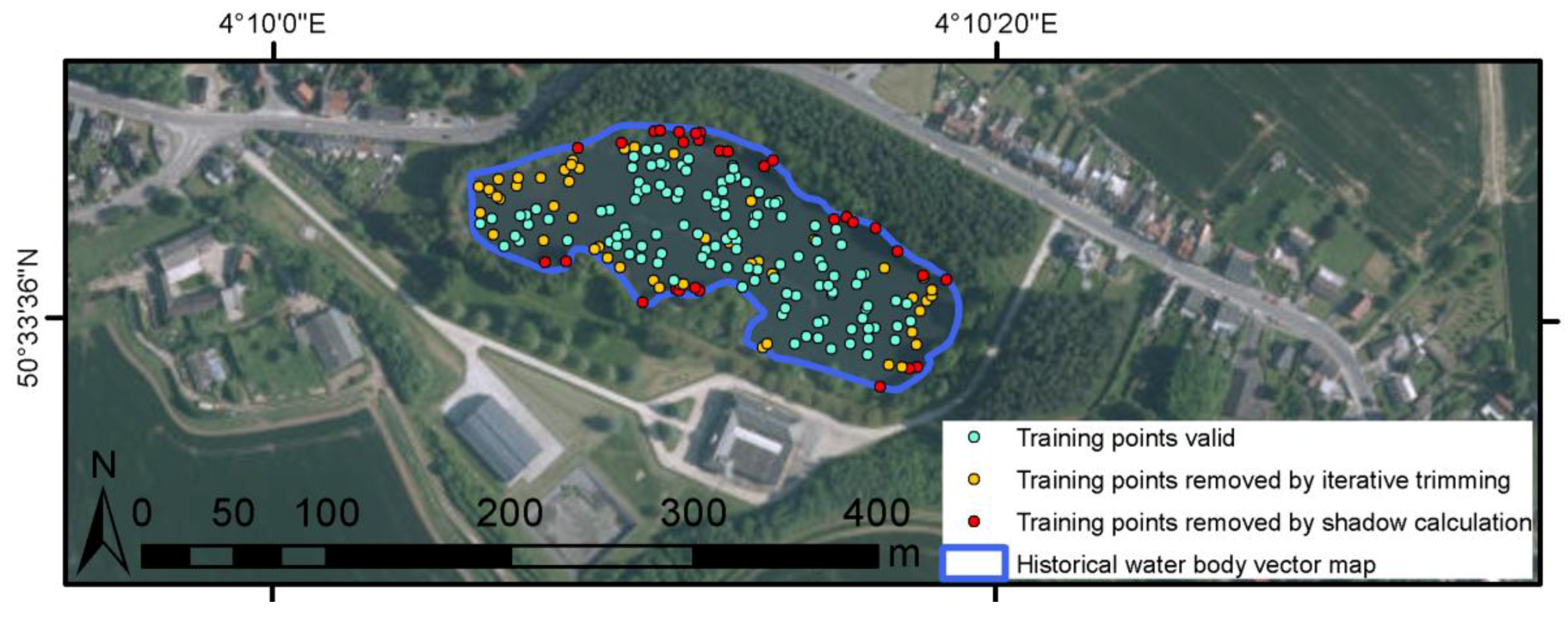
5.2.2. Random Sampling and Iterative Trimming to Remove Surface Affected by the Context

The results of the process of filtering the 200 sampling points for each historically-mapped water body are shown in Figure 11. From the 1,508,805 random points, about 1/3 are kept after removing points in shadow and after the multivariate iterative trimming. The result is 474,171 points in 6061 distinct water bodies.

5.3. Water Body Classification and Signal Processing Handling Intrinsic Variability of the Target

5.3.1. Aerial Photos Classification

The K-means 500 clusters classification is applied independently on each of the 36 strata. The aerial photos (Figure 12a) are in 500 clusters (Figure 12b). The mosaic bond-line is slightly visible on Figure 12a indicating two different acquisitions with different observation conditions. The classifiers are sensitive to this variability. Figure 12b reveals that more than five clusters correspond to the same water body. Using a huge number of clusters makes it possible to deal with the spectral variability of the water bodies.

After the clustering of each stratum into one of 500 clusters, the labeling makes it possible to select the water clusters among the 500 clusters. The clusters of the 474,171 points sampled are extracted separately for each stratum. For each stratum, the proportion of water sample points in each cluster is calculated. Each cluster with a proportion superior to 0.5% is then labeled as water. Throughout the 36 strata, the cluster number labeled as water varies from 1 to 26 per stratum with an average of 11 and a standard deviation of 5 (

Table 1. Statistics (minimum, quartiles, mean, maximum) of the stratum areas, the water body numbers, the water body areas, the labeling point numbers, and the number of clusters classified as water for the 36 strata.

	Stratum (Area km²)	Historical Water Body Vector Map Sampling		Classification
		Water Body (Number)	Water Body (Area m²)	Labeling Points (Number)	Water Cluster (Number)
Minimum	16	2	434.5	116	1
1st Quartile	190	77	1851.6	5465	8
Median	407.5	126	2662.4	9928	11
Mean	471.3	169	3198.7	13,171	11
3rd Quartile	701.5	243	4184.2	18,508	14
Maximum	1127	518	10,817.7	39,953	26

). After the labeling, the shadow is removed and morphological mathematics are applied. Finally, the raster is converted to a vector dataset containing 163,049 features.

5.3.2. LiDAR Signal Processing

The LiDAR LAS is processed using a Binning Maximum Simple interpolation to obtain the LiDAR intensity raster at 1-m resolution, which is in turn converted to water layer by thresholding the values (Figure 13). On the other hand, the LAS is processed using the Binning Maximum None interpolation to obtain no data layer. The water layer provides the water on which the LiDAR pulses were reflected and then thresholded as water. The no data layer provides all the surfaces where the pulses were absorbed or reflected away from the sensor. This layer thus contains many artifacts but also many water surfaces, as illustrated in Figure 13.

These two layers are then combined along with the application of morphological mathematics in seven steps summarized in

Table 2. LiDAR processing sequences with their corresponding surface water variations (percent %; the first layer is considered as 100% for comparison).

Order	1	2	3	4	5	6	7
operation	union of water and no data layers	eroded (3 m)	dilated (3 m)	union with water layer	dilated (2 m)	eroded (3 m)	dilated (1 m)
% surface water	100.00	87.75	88.07	88.10	88.40	88.00	82.04

. The water surface initially detected decreased by 17.96% to reach 82.04% of the surface of the initial water detection.

The resulting raster is then converted to a 57,921-polygon vector file.

5.4. Combinations and Update of the Water Body Map

Finally, the two layers are combined with a union summing detection (1 if detected only by one method and 2 if detected by both methods). The following steps then make it possible to prioritize the update in three layers while taking the best contours (Figure 14): Layer A (23,583 polygons), Layer B (34,338 polygons), and Layer C (134,542 polygons). Using three layers permits to benefit of the finest contour of the LiDAR. Layer A has the edges of LiDAR that are detected in both LiDAR and aerial photos, Layer B has the edges of LiDAR that are detected only by one method and that do not intersect with Layer A, and Layer C are the remaining polygons. Splitting the map update into those three layers permits us to prioritize the review of the results by an operator, presenting first high confidence detection and contour from Layer A to less confident detection and contour in Layer C. The three layers are finally combined after their revisions.

5.5. Quality Evaluation

Although the three layers (A, B, C) were finally combined, the quality evaluation is also done for each layer separately for the final result.

Table 3. Detection efficiency and detection cost for layer A, B, and C and for the different size classes of water bodies (25–50 m², 50–100 m², or greater than 100 m²). Layer A contains the water bodies detected by both LiDAR and aerial photos with the contour of the LiDAR. Layer B contains the remaining polygons detected by LiDAR only. Layer C contains the remaining polygons detected by aerial photo classification.

	<50 m²		50–100 m²		>100 m²		Total
	Detection Efficiency	Detection Cost	Detection Efficiency	Detection Cost	Detection Efficiency	Detection Cost	Detection Efficiency	Detection Cost
Layer A	6/330 (1.82%)	43/6 (7.17)	27/162 (16.67%)	73/27 (2.7)	540/843 (64.06%)	524/540 (0.97)	573/1334 (42.95%)	638/573 (1.11)
Layer B	16/330 (4.85%)	270/16 (16.88)	23/162 (14.2%)	334/23 (14.52)	132/843 (15.66%)	419/132 (3.17)	171/1334 (12.82%)	984/171 (5.75)
Layer C	42/330 (12.73%)	1878/42 (44.71)	28/162 (17.28%)	626/28 (22.36)	159/843 (18.86%)	671/159 (4.22)	229/1334 (17.17%)	2148/229 (9.38)
Total	64/330 (19.39%)	2191/64 (34.23)	78/162 (48.15%)	1033/78 (13.24)	831/843 (98.57%)	1614/831 (1.94)	973/1334 (72.93%)	3770/973 (3.87)

shows the results of detection efficiency and detection cost for the three resulting layers (A, B, C) for different sizes of water bodies. Among the total number (1334) of the water bodies identified over the 16 validation zones, 973 were detected (72.93%). The detection efficiency is higher for large water bodies, as 98.57% of the water bodies greater than 100 m² are well detected. Figure 15a–c illustrates good performance of the framework while commission errors greater than 100 m² are illustrated in Figure 15d–f. Case d was not detected because it was flagged as shadow and was thus removed. Most of them (such as e and f) have an atypical spectral signature (muddy, eutrophic, cover by vegetation).

When considering only the water bodies smaller than 50 m², the detection efficiency decreases to 19.39%. To explain the relatively weak result for very small water bodies, a visual check of the 266 water bodies not detected reveals that 62.4% (166) are swimming pools. Two facts explained why the detection of swimming pools is not efficient: (1) swimming pools are most of the time covered by a plastic canvas in Belgium and (2) the sampled points used to label the classification are not drawn in swimming pools, which may have an atypical spectral signature. If swimming pools are removed from the validation dataset, the framework is able to detect 83.3% of the water bodies and 39.02% of the water bodies smaller than 50 m².

6. Discussion

This study combines hyperspatial data sources of different types taken with heterogeneous observation conditions over large areas (17,000 km²). The framework and its components are discussed here along with their limitations and perspectives for future research.

No framework or method to map thematic land cover handling hyperspatial multi-source data over large areas was found in the literature despite their interest for managers and scientists. On the one hand, only one study at sub-metric resolution over large areas using airborne multispectral remote sensing techniques for geomorphological work in fluvial environments was published [23]. Nevertheless, the authors do not propose a framework able to deal with other data sources and with heterogeneities coming from observation and target. On the other hand, no data fusion handling heterogeneous data was proposed in the literature. In this framework, a decision-level fusion combining the results from multiple sources is proposed. By managing the heterogeneity of the data source separately through the stratification via the observation conditions mapping as well as the removal of surface affected by local heterogeneity, an innovative and generic framework usable with other platforms and for other thematic maps was proposed.

This research reveals the importance of managing the local neighborhood effects of the target, especially for shadow, as this covers about 30% of the whole area of the study. Up to now, there has been no easy and effective method for dealing with shadows at hyperspatial resolution over large areas, especially when the land cover target class is absorbing most of the visible spectra, such as in water or urban areas [58]. The confusion between shadow and water is an enduring problem for high-resolution images [69]. Figure 16 represents red, green, blue, near-infrared, NDVI, and NDWI variables in shadowed and non-shadowed parts of water bodies. This highlights the difficulty of separating shadow from band or index. Indeed, no existing water index can extract water information while at the same time suppressing the false alarm of shadow [70] as the values are too close. This problem increases while going through hyperspatial resolution as small objects create shadows that are not visible at coarser resolutions. The shadow modeling approach proposed in this study was possible because the geometry of scenes and light sources was known; however, similar approaches were already proposed in former studies [56,57,58]. Finally, this study reveals the need for precise and up-to-date DSM in future studies as it is a prerequisite for modeling shadows.

Among the data used to map water, the framework proposes the classification of aerial photos. Each 25-cm pixel has 256⁶ combination of values possible in six bands (red, green, blue, near-infrared, NDVI, and NDWI) are available with values ranging from 1–256. The proposed K-means clustering permits to reduce the dimension of the data from 256⁶ to 500 clusters in order to better estimate the frequency. The arbitrary choice of 500 clusters is quite unusual when considering the literature because there is a risk of overfitting with too large a number of classes. Overfitting could jeopardize generalization of the classification to broader scale. In the current study, the clustering and labeling are applied locally on each stratum, which makes the overfitting on the local stratum almost desirable to characterize the local spectral heterogeneity of the water bodies. There is no a priori method to evaluate the ideal number of clusters. A possible way to estimate the optimal number of clusters in future studies is to iteratively classify the data with a varying cluster number and compare the validation results at each step. In addition to the clustering, the sampling number and location in the historical water body vector map are crucial for a correct labeling of the clusters. In this study, 474,171 points in 6061 water bodies were used, while there are about 40,000 water bodies in the study region. First the existence of water bodies in the historical map is confirmed. Then a 200-point sampling with 1-m minimum distance is trimmed to remove outliers. At the end of the process, small and heterogeneous water bodies could be discarded from the labeling points to limit cluster labeling of atypical water bodies and thus their detection. As an illustration, after the trimming of the data, the smallest water body sampled is 434.5 m² (Table 1); this could explain the limited performance for detection of water bodies smaller than 100 m². Another limitation of the approach is the heterogeneity of the stratum areas. Among the 36 strata, the average area is 471 km² but the smallest covers only 16 km² (Table 1). This small stratum has a limited number of water bodies for the sampling and only 116 labeling points are available, while an average stratum has about 13,000 points. In future research, a stratum that is too small should be re-aggregated with its neighbors. Research on labeling points distribution with relation to the size and the heterogeneity of water could potentially improve the results. In addition to the cluster number and the labeling points, the super-computing facility required to process the data could limit the framework’s usefulness. A workaround tested, but not described in this study, was to decrease the resolution from 25 cm to 2 m, reducing the processing time by a factor of 64 and making it usable on a normal computer. The framework was working fine but water delineation was logically not sub-metric. In conclusion, aerial photo classification clustering is a powerful, simple method to reduce the dimension of a dataset without a priori knowledge. Its labeling with historical data provides good results as long as the labeling data are well distributed and representative of the local water bodies. Future researches should focus on improving the robustness of the sampling used for labeling, especially for very small water bodies.

A combination of sources of data is particularly suited as it has already been highlighted in much research [12,34,37,41,43]. In particular, LiDAR is able to penetrate the canopy and is thus more accurate in delineating the water bodies. However, it misses some water bodies as the laser pulse can be reflected. Additionally, the LiDAR pulse density is critical, especially in forested areas where water bodies are difficult to detect on aerial photos and LiDAR. When the LiDAR density falls between 0 and 1 point/m² (Figure 5), it means that it is not possible to detect water below meter. On the other hand, the aerial photos offer a higher resolution (25 cm) and improve or decrease the confidence of the detection from LiDAR. The combination of data sources remains a challenge for the remote sensing community and few studies have put forward an operational framework for water mapping. The proposed framework is well suited to addressing this challenge.

In this study, morphological mathematics were used for artifact reduction and water gap filling. For both aerial photo classification and LiDAR, the morphological mathematics operations were useful. Their effects on surfaces were outlined for LiDAR with 12.25% surface lost with the first 3-m erosion applied, and a total of 17.96% of surfaces lost after all the steps (Table 2). In this study, the rationale was always the same: a 1-m opening operation (erosion followed by dilation) permits us to remove lonely pixel artifacts and a 3-m closure operation (dilation followed by erosion) permits us to fill the gaps in the water bodies. Those morphological operations result in a limitation of the approach to detect water bodies smaller than 3 × 3 m. Moreover, islands smaller than 9 m² could be removed by filling gaps that are not gaps. Future research on morphological mathematics applications and on the optimal configuration of the kernel size could formalize those operations according to the objective of the study and its landscape structure.

Another point to discuss is the usefulness of hyperspatial resolution with regards to the performance achieved and the lower-resolution imagery available. Clearly, as demonstrated in the introduction, having hyperspatial resolution map is useful for managers, engineers, and scientists. However, the framework complexity along with the acquisition period (here almost three years) could bring into question the value of using the proposed approach in place of available lower-resolution imagery. First, a distinction should be made between detection, which is the presence or absence of water, and delineation, which is the contour of water. This framework focuses on delineation and although all the water bodies are not detected with the approach, the ones detected have a delineation at 1-m resolution. The proposed approach detects 98.57% of water bodies greater than 100 m² with a sub-metric accuracy delineation. A study [24] on the same region demonstrates that the smallest water body detectable with the 10-m Sentinel-2 bands was 11 m in diameter. Thus, even with the finest Sentinel-2 bands, it is not possible to detect water bodies smaller than 100 m². The framework is able to detect 48.15% of water bodies smaller between 50 and 100 m², with a 1-m delineation. In addition, this framework was used by the administration to reduce their manual update work as they need to map water bodies from 25 m² as they are eligible for subsidies in the context of the CAP. Future research on improving the accuracy of water contour estimation could help us to quantify and compare the proposed approaches.

Although the amount of manual mapping work has decreased as most water bodies are well delineated by the framework with a precision higher than 1 m, this study reveals that an operator is still valuable to check and validate the water bodies. For water bodies greater than 100 m² the operator was able to use the resulting layers, obtaining a 98.57% rate of detection success. For smaller water bodies (<50 m²), the efficiency decreases to 39.02% if swimming pools are not taken into account.

The validation scheme used in the study, i.e., stratified random sampling, provides a valuable assessment of the results. However, as the stratification is based on aerial photo acquisition, the stratification does not really provide complementary information for the validation. Therefore, a future validation scheme should not necessarily be stratified but only requires random sampling. Moreover, based on photo interpretation of aerial photography, the validation dataset quality could be impacted by the quality of the aerial photos, which also impacts the classification results. Therefore, independent ground truth sampling would be more appropriate even if it is difficult to obtain. In addition to the validation of the water presence, a validation of the contour could also be particularly interesting for future research, especially at hyperspatial resolution.

The framework could be applied to data acquired by aircraft, satellite, and drones. The recent digital revolution in aerial photos brings satellite methodologies to aerial photos. The proposed framework addressed this challenge over large areas. After questioning some commercial satellite data providers, it appears that currently few commercial providers are able to meet the acquisition specifications—spatial resolution below 1 meter, “cloud-free” data, and acquisition between 1 April and 1 July (to capture the start of the crop growing season). Up to now, commercial satellites such as Deimos-2 and WorldView-3 have a panchromatic resolution below 1 m at nadir but are not able to cover large areas with the acquisition specifications. The proposed framework is suited to handling heterogeneous satellite mosaics that will be available on larger areas in the future.

Additionally, the proposed method could also be applied to Unmanned Aerial Vehicle (UAV) imagery processing. Shahbazi et al. reviewed UAV applications and water bodies play a large part as UAVs were used for mapping aquatic species and characterizing water bodies. Aerial remote sensing and UAV have similar constraints. In the light of the application reviewed [71], the radiometric inconsistency of images should be adjusted, and geometric errors need to be duly rectified to produce satisfying results. The proposed framework could reduce this work of image adjustment by mapping the acquisition conditions as a prerequisite to classification.

Finally, the proposed framework could also be applied to other land features. For instance, urban areas are difficult to map because of the intrinsic heterogeneity of the buildings, as well as road networks, houses, and other artificial surfaces. Furthermore, the neighborhood effects of the buildings could be handled in the same way as in the current study.

7. Conclusions

The paper describes a framework and its application to handling the heterogeneity of remote sensing platforms (UAV, aircraft, satellite), sensors (optical, LiDAR, SAR) and observation conditions (VZA, SZA, date). The proposed framework further deals with the water within-type diversity (morphology, origin, composition) and with the neighborhood effects (shadow) target water bodies. Such a framework is suited to mapping thematic land features over large areas with hyperspatial resolution. The proposed framework detects 83% of water bodies—if swimming pools are not taken into account—and more than 98% of those water bodies greater than 100 m², with an edge accuracy below 1 m over large areas. This study opens avenues for operational application at a regional scale.

References

- Greenberg, J.; Dobrowski, S.; Ustin, S. Shadow allometry: Estimating tree structural parameters using hyperspatial image analysis. Remote Sens. Environ. 2005, 97, 15–25. [Google Scholar] [CrossRef]
- Rocchini, D.; Balkenhol, N.; Carter, G.A.; Foody, G.M.; Gillespie, T.W.; He, K.S.; Kark, S.; Levin, N.; Lucas, K.; Luoto, M.; et al. Remotely sensed spectral heterogeneity as a proxy of species diversity: Recent advances and open challenges. Ecol. Inform. 2010, 5, 318–329. [Google Scholar] [CrossRef]
- Davis, T. The Ramsar Convention Manual: A Guide to the Convention on Wetlands of International Importance Especially as Waterfowl Habitat; Ramsar Convention Bureau: Gland, Switzerland, 1994. [Google Scholar]
- Verhoeven, J.T.A. Wetlands in Europe: Perspectives for restoration of a lost paradise. Ecol. Eng. 2014, 66, 6–9. [Google Scholar] [CrossRef]
- Holgerson, M.A.; Raymond, P.A. Large contribution to inland water CO2 and CH4 emissions from very small ponds. Nat. Geosci. 2016, 9, 222–226. [Google Scholar] [CrossRef]
- Marton, J.M.; Creed, I.F.; Lewis, D.B.; Lane, C.R.; Basu, N.B.; Cohen, M.J.; Craft, C.B. Geographically Isolated Wetlands are Important Biogeochemical Reactors on the Landscape. Bioscience 2015, 65, 408–418. [Google Scholar] [CrossRef]
- Hefting, M.M.; van den Heuvel, R.N.; Verhoeven, J.T.A. Wetlands in agricultural landscapes for nitrogen attenuation and biodiversity enhancement: Opportunities and limitations. Ecol. Eng. 2013, 56, 5–13. [Google Scholar] [CrossRef]
- Dudgeon, D.; Arthington, A.H.; Gessner, M.O.; Kawabata, Z.-I.; Knowler, D.J.; Lévêque, C.; Naiman, R.J.; Prieur-Richard, A.-H.; Soto, D.; Stiassny, M.L.J.; et al. Freshwater biodiversity: Importance, threats, status and conservation challenges. Biol. Rev. 2006, 81, 163–182. [Google Scholar] [CrossRef] [PubMed]
- Sala, O.E.; Chapin, F.S.; Armesto, J.J.; Berlow, E.; Bloomfield, J.; Dirzo, R.; Huber-Sanwald, E.; Huenneke, L.F.; Jackson, R.B.; Kinzig, A.; et al. Global biodiversity scenarios for the year 2100. Science (80-) 2000, 287, 1770–1774. [Google Scholar] [CrossRef]
- Collen, B.; Whitton, F.; Dyer, E.E.; Baillie, J.E.M.; Cumberlidge, N.; Darwall, W.R.T.; Pollock, C.; Richman, N.I.; Soulsby, A.-M.; Böhm, M. Global patterns of freshwater species diversity, threat and endemism. Glob. Ecol. Biogeogr. 2014, 23, 40–51. [Google Scholar] [CrossRef] [PubMed]
- Brönmark, C.; Hansson, L.-A. Environmental issues in lakes and ponds: Current state and perspectives. Environ. Conserv. 2002, 29, 290–306. [Google Scholar] [CrossRef]
- Wu, Q.; Lane, C.; Liu, H. An Effective Method for Detecting Potential Woodland Vernal Pools Using High-Resolution LiDAR Data and Aerial Imagery. Remote Sens. 2014, 6, 11444–11467. [Google Scholar] [CrossRef]
- Alsdorf, D.E.; Rodriguez, E.; Lettenmaier, D.P. Measuring surface water from space. Rev. Geophys. 2007, 45. [Google Scholar] [CrossRef]
- Alsdorf, D.E.; Lettenmaier, D.P. Tracking Fresh Water from Space. Science (80-) 2003, 301, 1491–1494. [Google Scholar] [CrossRef] [PubMed]
- Famiglietti, J.; Cazenave, A.; Eicker, A.; Reager, J. Satellites provide the big picture. Science 2015, 349, 684–685. [Google Scholar] [CrossRef] [PubMed]
- Palmer, S.; Kutser, T.; Hunter, P. Remote sensing of inland waters: Challenges, progress and future directions. Remote Sens. Environ. 2015, 157, 1–8. [Google Scholar] [CrossRef]
- Marcus, W.A.; Fonstad, M.A. Optical remote mapping of rivers at sub-meter resolutions and watershed extents. Earth Surf. Process. Landf. 2008, 33, 4–24. [Google Scholar] [CrossRef]
- Dörnhöfer, K.; Oppelt, N. Remote sensing for lake research and monitoring—Recent advances. Ecol. Indic. 2016, 64, 105–122. [Google Scholar] [CrossRef]
- Marcus, W.; Legleiter, C.; Aspinall, R.; Boardman, J. High spatial resolution hyperspectral mapping of in-stream habitats, depths, and woody debris in mountain streams. Geomorphology 2003, 55, 363–380. [Google Scholar] [CrossRef]
- Lejot, J.; Delacourt, C.; Piégay, H.; Fournier, T.; Trémélo, M.-L.; Allemand, P. Very high spatial resolution imagery for channel bathymetry and topography from an unmanned mapping controlled platform. Earth Surf. Process. Landf. 2007, 32, 1705–1725. [Google Scholar] [CrossRef]
- Goovaerts, P. Geostatistical incorporation of spatial coordinates into supervised classification of hyperspectral data. J. Geogr. Syst. 2002, 4, 99–111. [Google Scholar] [CrossRef]
- Carbonneau, P.; Lane, S.; Bergeron, N. Feature based image processing methods applied to bathymetric measurements from airborne remote sensing in fluvial environments. Earth Surf. Process. Landf. 2006, 31, 1413–1423. [Google Scholar] [CrossRef]
- Carbonneau, P.E.; Lane, S.N.; Bergeron, N.E. Catchment-scale mapping of surface grain size in gravel bed rivers using airborne digital imagery. Water Resour. Res. 2004, 40. [Google Scholar] [CrossRef] [Green Version]
- Marcus, W.A.; Crabtree, R.; Aspinall, R.J.; Boardman, J.W.; Despain, D.; Minshall, W.; Peel, J. Validation of High-Resolution Hyperspectral Data for Stream and Riparian Habitat Analysis; Annual Report (Phase 2) to NASA EOCAP Program; Stennis Space Flight Center: Hancock County, MS, USA, 2000.
- Li, L.; Chen, Y.; Yu, X.; Liu, R.; Huang, C. Sub-pixel flood inundation mapping from multispectral remotely sensed images based on discrete particle swarm optimization. ISPRS J. Photogramm. Remote Sens. 2015, 101, 10–21. [Google Scholar] [CrossRef]
- Manakos, I.; Chatzopoulos-Vouzoglanis, K.; Petrou, Z.; Filchev, L.; Apostolakis, A. Globalland30 Mapping Capacity of Land Surface Water in Thessaly, Greece. Land 2014, 4, 1–18. [Google Scholar] [CrossRef]
- Sakthivel, S.P.; Genitha C., H.; Sivalingam, V.J.; Shanmugam, S. Super-resolution mapping of hyperspectral images for estimating the water-spread area of Peechi reservoir, southern India. J. Appl. Remote Sens. 2014, 8, 83510. [Google Scholar] [CrossRef]
- Foody, G.M.; Muslim, A.M.; Atkinson, P.M. Super-resolution mapping of the waterline from remotely sensed data. Int. J. Remote Sens. 2005, 26, 5381–5392. [Google Scholar] [CrossRef]
- Muster, S.; Heim, B.; Abnizova, A.; Boike, J. Water Body Distributions Across Scales: A Remote Sensing Based Comparison of Three Arctic TundraWetlands. Remote Sens. 2013, 5, 1498–1523. [Google Scholar] [CrossRef] [Green Version]
- Kay, S.; Hedley, J.; Lavender, S. Sun glint correction of high and low spatial resolution images of aquatic scenes: A review of methods for visible and near-infrared wavelengths. Remote Sens. 2009. [Google Scholar] [CrossRef]
- Gallant, A. The Challenges of Remote Monitoring of Wetlands. Remote Sens. 2015, 7, 10938–10950. [Google Scholar] [CrossRef]
- Campbell, J.B.; Wynne, R.H. Introduction to Remote Sensing; Guilford Press: New York, NY, USA, 2011. [Google Scholar]
- Rautiainen, M.; Nilson, T.; Lang, M.; Kuusk, A.; Mo, M. Canopy gap fraction estimation from digital hemispherical images using sky radiance models and a linear conversion method. Agric. For. Meteorol. 2010, 150, 20–29. [Google Scholar]
- Lichvar, R.; Finnegan, D.; Newman, S.; Ochs, W. Delineating and Evaluating Vegetation Conditions of Vernal Pools Using Spaceborne and Airborne Remote Sensing Techniques; Beale Air Force Base: Marysville, CA, USA, 2006. [Google Scholar]
- Brzank, A.; Heipke, C. Classification of Lidar Data into water and land points in coastal areas. Int. Arch. Photogramm. 2006, 9, 197–202. [Google Scholar]
- Höfle, B.; Vetter, M.; Pfeifer, N.; Mandlburger, G.; Stötter, J. Water surface mapping from airborne laser scanning using signal intensity and elevation data. Earth Surf. Process. Landf. 2009, 34, 1635–1649. [Google Scholar] [CrossRef]
- Hodgson, M.E.; Jensen, J.R.; Tullis, J.A.; Riordan, K.D.; Archer, C.M. Synergistic Use of Lidar and Color Aerial Photography for Mapping Urban Parcel Imperviousness. Photogramm. Eng. Remote Sens. 2003, 69, 973–980. [Google Scholar] [CrossRef]
- Chen, Y.; Su, W.; Li, J.; Sun, Z. Hierarchical object oriented classification using very high resolution imagery and LIDAR data over urban areas. Adv. Space Res. 2009, 43, 1101–1110. [Google Scholar] [CrossRef]
- Bork, E.W.; Su, J.G. Integrating LIDAR data and multispectral imagery for enhanced classification of rangeland vegetation: A meta analysis. Remote Sens. Environ. 2007, 111, 11–24. [Google Scholar] [CrossRef]
- Rodríguez-Cuenca, B.; Alonso, M. Semi-Automatic Detection of Swimming Pools from Aerial High-Resolution Images and LIDAR Data. Remote Sens. 2014, 6, 2628–2646. [Google Scholar] [CrossRef]
- Maxa, M.; Bolstad, P. Mapping northern wetlands with high resolution satellite images and LiDAR. Wetlands 2009, 29, 248–260. [Google Scholar] [CrossRef]
- Lang, M.W.; McCarty, G.W. Lidar intensity for improved detection of inundation below the forest canopy. Wetlands 2009, 29, 1166–1178. [Google Scholar] [CrossRef]
- Elaksher, A.F. Fusion of hyperspectral images and lidar-based dems for coastal mapping. Opt. Lasers Eng. 2008, 46, 493–498. [Google Scholar] [CrossRef]
- Bigdeli, B.; Samadzadegan, F.; Reinartz, P. A decision fusion method based on multiple support vector machine system for fusion of hyperspectral and LIDAR data. Int. J. Image Data Fusion 2014, 5, 196–209. [Google Scholar] [CrossRef]
- Zhu, X.; Chen, J.; Gao, F.; Chen, X.; Masek, J.G. An enhanced spatial and temporal adaptive reflectance fusion model for complex heterogeneous regions. Remote Sens. Environ. 2010, 114, 2610–2623. [Google Scholar] [CrossRef]
- Zhang, J. Multi-source remote sensing data fusion: Status and trends. Int. J. Image Data Fusion 2010. [Google Scholar] [CrossRef]
- Graitson, E. Elaboration d’un Référentiel et de Documents de Vulgarisation sur les Mares Agricoles en Région Wallonne; Rapport Final—Partie 2; ORBi: Liège, Belgium, 2009. [Google Scholar]
- Kristensen, P.; Globevnik, L. European Small Water Bodies. Biol. Environ. Proc. R. Irish Acad. 2014, 114B, 281–287. [Google Scholar] [CrossRef]
- Ernst, J.; Dewals, B.J.; Archambeau, P.; Detrembleur, S.; Erpicum, S.P.M. Integration of accurate 2D inundation modelling , vector land use database and economic damage evaluation. Flood Risk Manag. Res. Pract. 2008, 1643–1653. [Google Scholar]
- Gouvernement Wallon. Direction Générale de l’Agriculture des Ressources Naturelles et de l’Environnement (Service Public Wallonie) PICEA; Projet du Gouvernement Wallon; Gouvernement Wallon: Namur, Belgium, 2006; Volume GW VIII.
- Triggs, B.; Mclauchlan, P.; Hartley, R.; Fitzgibbon, A. Bundle Ajustment—A Modern Synthesis. Lect. Notes Comput. Sci. 2000, 1883, 298–372. [Google Scholar]
- Service Public Wallonnie (SPW). Orthophotos 2012–2013 Rapport de Production Orthophotos Couleur Numériques d’une Résolution de 25 cm; Service Public Wallonnie (SPW): Jambes, Belgium, 2013. [Google Scholar]
- Roy, D.P.; Ju, J.; Kline, K.; Scaramuzza, P.L.; Kovalskyy, V.; Hansen, M.; Loveland, T.R.; Vermote, E.; Zhang, C. Web-enabled Landsat Data (WELD): Landsat ETM+ composited mosaics of the conterminous United States. Remote Sens. Environ. 2010, 114, 35–49. [Google Scholar] [CrossRef]
- Open Geospatial Consortium. G.D.T. GDAL—Geospatial Data Abstraction Library; Open Source Geospatial Foundation: Chicago, IL, USA, 2015. [Google Scholar]
- Shahtahmassebi, A.; Yang, N.; Wang, K.; Moore, N.; Shen, Z. Review of shadow detection and de-shadowing methods in remote sensing. Chin. Geogr. Sci. 2013, 23, 403–420. [Google Scholar] [CrossRef]
- Nakajima, T.; Tao, G.; Yasuoka, Y. Simulated recovery of information in shadow areas on IKONOS image by combing ALS data. In In Proceeding of the Asian Conference on Remote Sensing (ACRS), Kathmandu, Nepal, 25–29 November 2002; Available online: http://a-a-r-s.org/aars/proceeding/ACRS2002/Papers/VHR02-2.pdf (accessed on 23 February 2017).
- Zhan, Q.; Shi, W.; Xiao, Y. Quantitative analysis of shadow effects in high-resolution images of urban areas. Sūgaku 2012, 11, 97–110. [Google Scholar]
- Dare, P.M. Shadow Analysis in High-Resolution Satellite Imagery of Urban Areas. Photogramm. Eng. Remote Sens. 2005, 71, 169–177. [Google Scholar] [CrossRef]
- McFEETERS, S.K. The use of the Normalized Difference Water Index (NDWI) in the delineation of open water features. Int. J. Remote Sens. 1996, 17, 1425–1432. [Google Scholar] [CrossRef]
- Environmental Systems Research Institute. ESRI ArcGIS Desktop—Version 13; Environmental Systems Research Institute: Redlands, CA, USA, 2016. [Google Scholar]
- Tucker, C.J. Red and photographic infrared linear combinations for monitoring vegetation. Remote Sens. Environ. 1979, 8, 127–150. [Google Scholar] [CrossRef]
- Mahalanobis, P. On the generalized distance in statistics. Proc. Natl. Inst. Sci. 1936, 2, 49–55. [Google Scholar]
- Richards, J.A. Remote Sensing Digital Image Analysis; Springer: Berlin/Heidelberg, Germany, 2013. [Google Scholar]
- Radoux, J.; Defourny, P. Automated image-to-map discrepancy detection using iterative trimming. Photogramm. Eng. Remote Sens. 2010, 76, 173–181. [Google Scholar] [CrossRef]
- Desclée, B.; Bogaert, P.; Defourny, P. Forest change detection by statistical object-based method. Remote Sens. Environ. 2006, 102, 1–11. [Google Scholar] [CrossRef]
- Matton, N.; Canto, G.; Waldner, F.; Valero, S.; Morin, D. An automated method for annual cropland mapping along the season for various globally-distributed agrosystems using high spatial and temporal resolution. Remote Sens. 2015, 7, 13208–13232. [Google Scholar] [CrossRef]
- Inglada, J.; Christophe, E. The Orfeo Toolbox Remote Sensing Image Processing Software. In Proceedings of the 2009 IEEE International Geoscience and Remote Sensing Symposium, Cape Town, South Africa, 12–17 July 2009; pp. 733–736.
- Hallot, P.; Billen, R. Rapport Final Reengineering PICC S0. 04.01-11PNSP-01; ORBi: Liège, Belgium, 2013. [Google Scholar]
- Nath, R.K.; Deb, S.K. Water-Body Area Extraction From High Resolution Satellite Images-An Introduction, Review, and Comparison. Int. J. Image Process. 2010, 3, 353–372. [Google Scholar]
- Xie, C.; Huang, X.; Zeng, W.; Fang, X. A novel water index for urban high-resolution eight-band WorldView-2 imagery. Int. J. Digit. Earth 2016, 9, 925–941. [Google Scholar] [CrossRef]
- Shahbazi, M.; Théau, J.; Ménard, P. Recent applications of unmanned aerial imagery in natural resource management. Gisci. Remote Sens. 2014, 51, 339–365. [Google Scholar] [CrossRef]