A Comparison of MODIS/VIIRS Cloud Masks over Ice-Bearing River: On Achieving Consistent Cloud Masking and Improved River Ice Mapping

Abstract

The capability of frequently and accurately monitoring ice on rivers is important, since it may be possible to timely identify ice accumulations corresponding to ice jams. Ice jams are dam-like structures formed from arrested ice floes, and may cause rapid flooding. To inform on this potential hazard, the CREST River Ice Observing System (CRIOS) produces ice cover maps based on MODIS and VIIRS overpass data at several locations, including the Susquehanna River. CRIOS uses the respective platform’s automatically produced cloud masks to discriminate ice/snow covered grid cells from clouds. However, since cloud masks are produced using each instrument’s data, and owing to differences in detector performance, it is quite possible that identical algorithms applied to even nearly identical instruments may produce substantially different cloud masks. Besides detector performance, cloud identification can be biased due to local (e.g., land cover), viewing geometry, and transient conditions (snow and ice). Snow/cloud confusions and large view angles can result in substantial overestimates of clouds and ice. This impacts algorithms, such as CRIOS, since false cloud cover precludes the determination of whether an otherwise reasonably cloud free grid consists of water or ice. Especially for applications aiming to frequently classify or monitor a location it is important to evaluate cloud masking, including false cloud detections. We present an assessment of three cloud masks via the parameter of effective revisit time. A ~100 km stretch of up to 1.6 km wide river was examined with daily data sampled at 500 m resolution, examined over 317 days during winter. Results show that there are substantial differences between each of the cloud mask products, especially while the river bears ice. A contrast-based cloud screening approach was found to provide improved and consistent cloud and ice identification within the reach (95%–99% correlations, and 3%–7% mean absolute differences) between the independently observing platforms. River ice was also detected accurately (proportion correct 95%–100%) and more frequently. Owing to cross-platform compositing, it is possible to obtain an effective revisit time of 2.8 days and further error reductions.

1. Introduction

1.1. Spaceborne Monitoring of Ice-Bearing Rivers

The Moderate Resolution Imaging Spectroradiometer (MODIS) and the Visible Infrared Imaging Radiometer Suite (VIIRS) instruments, owing to large observing swaths and polar orbits, allow for daily or better global coverage at up 250 and 375 m spatial resolutions, respectively. Frequent observations are desirable to monitor ice-bearing rivers, since ice jams may cause flooding within hours. It is also important to observe wide swaths, since hydrometric stations have greatly declined in number since the 1980s [1,2], and may by themselves not provide adequate coverage for flood warning or detection. With respect to ice jams, it is important to know the river condition over an extended area up- and downstream of the jam. In light of flood detection being a vital and current issue, the Joint Polar Satellite System (JPSS) Proving Ground and Risk Reduction (PGRR) program supports two relevant satellite products derived from VIIRS: (1) a flood product [3]; and (2) a river ice product based on the CREST River Ice Observing algorithm (CRIOS) that was originally developed based on MODIS borne on Terra (MODIS-Terra) data [4]. Both products are hosted at the Space Science and Engineering Center (SSEC) of the University of Wisconsin at Madison (Available at: http://realearth.ssec.wisc.edu/; under “all”, “JPSS—FLOOD & ICE”).

1.2. Obtaining a Binary Cloud Mask from NASA Processing

Being optically-based, surface observations via MODIS and VIIRS are generally limited to cloud-free conditions. Most automatically generated and derived products rely on cloud masks to identify locations where grid cells are not impacted by clouds. The cloud mask is an output of globally calibrated cloud detection algorithms, consisting of a series of spectral tests using data from the particular instrument and other ancillary data, such as a land/water mask and snow/ice background flags as inputs. The algorithm used to generate the cloud product for MODIS, MOD35, consists of more than 20 spectral tests at different wavelengths and up to 250 m resolution [5]. Test results are processed, sampled to a 1 km resolution grid and categorized into four classes, also referred to as the unobstructed field-of-view (FOV) flags: confidently cloudy, mixed, not set (assumed clear) and confidently clear. In certain settings, different groupings may be more suitable, and custom cloud masks may be built based on individual MOD35 tests [6,7]. The most common approach is probably to take the “confidently clear” and “not set” categories to represent clear-sky while the remaining two are considered cloudy—thus producing a binary cloud mask. The cloud mask for VIIRS (VCM) is produced similarly [8]. The accuracy of any given cloud mask is critical, as many of the automatically generated downstream products depend on it. Beyond automatically generated products, cloud masks can be similarly critical to other products that rely on them such as the JPSS-PGRR river ice and flood maps. The cloud products for MODIS (MOD35) and VIIRS (VCM) are produced by NASA. For this particular research it is necessary to adopt a means to clearly identify which cloud mask was applied to which instrument. Specifically, the following designations will be used to refer to a binary cloud mask developed from a standard grouping (as above) of the unobstructed FOV flags contained within MOD35, MYD35 and the VCM: NASA(Terra), NASA(Aqua) and NASA(VIIRS), respectively.

1.3. Detection of (Near) Invisible Clouds Limits River Ice Monitoring

Accurate identification of opaque clouds over a narrow body of water (river) in winter may be especially challenging due to (1) difficulties in cloud/snow discrimination [9,10,11], especially relating to MODIS-Aqua [12,13]; (2) viewing geometry impacts: sensor zenith angle, solar elevation, and relative azimuth angle [14,15]; (3) biases related to land cover transitions [16] and grid cells containing both land and water; and (4) other issues such as navigation errors, accuracy of the land/water mask and resolution differences [11,17]. These challenges present valid concerns for river ice monitoring: the river and its bordering land may undergo considerable spectral change over a short time due to snow and ice; the land surface is interrupted by usually only a few grid cell wide body of water; and snow and ice are view dependent (anisotropic) reflectors. Further differences may be due to the algorithm design: for example, the MODIS cloud product is known to produce a more cloud conservative mask (it errs on the side of clouds) over snow cover [6]. As a result, the end user will have a reliable set of cloud-free data (“probably clear” and “confidently clear”), but at the cost of fewer-than-possible reasonably unobstructed grids to sample from. Thus, cloud overestimations such as “invisible” clouds have been noted [9], and literature features suggestions on how MOD35 cloud overestimates over snow might be reduced [6,7,11]. In our prior investigation, cloud cover overestimates in NASA(Aqua) were found to greatly limit river ice monitoring. We observed that only one full river observation every seven days was possible during snow cover, compared to one every four days otherwise [12]. Muhammad et al. [18] also noted problems with MODIS cloud masking: they originally used both MODIS snow products to map river ice along the Mackenzie river. To mitigate MODIS cloud overestimations and to avoid the MODIS cloud mask, threshold-based classification of radiance data were used at locations where the snow (and cloud) product indicated clouds.

1.4. Overview of Important Factors Pertaining to NASA Processing for MODIS and VIIRS

There are significant differences due to algorithms, ancillary data sources and current instrument capabilities. All of the NASA processing share in common that, at first, a processing path must be determined. The processing path for cloud detection depends on the best estimate of underlying (current) land cover and other relevant conditions: whether a grid is land, desert, water or coastal, snow/ice, prone to sun glint and whether the scene is sampled at night or during the day [7]. The VCM features even more possible processing paths. Relevant to this investigation is that the water class has a separate processing path for sea water and inland water in the VCM, which MOD35 does not [8,19]. As explained in Wilson et al. [16], the processing paths should be thought of as the specific suite of band tests for clouds that will be applied at a given grid. For example, MOD35 uses the Near-real-time Ice and Snow Extent (NISE) from the National Snow and Ice Data Center (NSIDC) to set the snow/ice processing flag, whereas the VCM obtains its background flag from its own product [8]. As noted in Thompson et al. [11], there is an issue of scale for MOD35, as the NISE is based on 25 km by 25 km observations of the Special Sensor Microwave Imager (SSMI/I). Thus, partial snow cover may not be detected, MODIS would not apply the relevant spectral test needed to discriminate clouds from snow or ice, and snow/ice would be detected as clouds. Consistent with this observation snow/cloud confusions may occur at the edge of snow cover, but cloud and snow overestimations are also attributable to large viewing angles and anisotropic scattering (especially forward scattering) which is also enhanced due to lower sun elevations occurring in winter [10,14,15].

Although exact processing pathways and individual tests are different, the principal test common to all approaches is the Normalized Difference Snow Index (NDSI), based on the 0.55 μm and 1.6 μm bands [20]. There is also a modified thresholding for NDSI based on the Normalized Difference Vegetation Index (NDVI) which is used to improve snow detection in forests [21]. The results of a preliminary NDSI test and the ancillary data flag are used to determine whether a snow/ice processing path is used for cloud detection. With respect to our study, it is important to emphasize that NDSI is tuned mainly for snow and snow/cloud discrimination rather than identification of ice. Ice and snow have similar, but not exactly the same optical properties (e.g., USGS (Available at http://pubs.usgs.gov/pp/p1386a/gallery2-fig77.html)), and the selected NDSI thresholds are likely not ideal for river ice identification or ice/cloud discrimination.

It is important to note that only MODIS-Aqua experienced a failure of the majority of its 1.6 μm detectors, and that the NDSI test for MODIS-Aqua instead uses band 7 (2.1 μm), which is also suitable for snow/cloud discrimination [11,22,23]. However, the NDSI/NDVI decision region is not used [13]. While producing generally similar snow (and by extension, cloud) products, differences between MOD10 and MYD10 are more apparent at less favorable viewing conditions [13]. Owing to this deficiency, approaches to statistically reconstruct the 1.6 μm band for MODIS-Aqua have been investigated [24,25,26,27]. With Collection 6 re-processing, a re-constructed band 6 is being used for MYD10, but not MYD35, product generation. It also features a higher resolution land/water mask [17] and other changes that may impact cloud masking or surface reflectance data. Owing to impacts on cloud and ice detection, a brief comparison between collection 5 to collection 6 differences is also provided in this study.

VIIRS features a novel along-scan aggregation of subpixel detectors to limit footprint growth. This allows for more consistent sampling of river-only grids. Although data may be sampled to a specific grid point, clearly located within the river, when sampled at large angles the at-grid reflectance magnitude may deviate due to adjacent snow or cloud cover if any are located within the observing footprint. Specifically, the VIIRS 375 m (nadir) bands may grow up to 0.8 km resolution, whereas the MODIS 500 m (nadir) bands may grow to 2.4 km resolution at the edge of scan [28,29].

1.5. Motivation and Novelty

Although results of NASA processed datasets are expected to differ somewhat, these approaches have the common goal of accurately identifying clouds: at minimum, in such a way that those data identified as “confidently clear” are in fact clear of clouds. Better would be an approach that does this while not substantially overestimating clouds. Even better would be an approach that purposefully ignores those semitransparent clouds that would ultimately not produce significant errors with respect to beneath-cloud land surface classifications.

Due to potential biases and errors in processed data, schemes that avoid such data are clearly preferred, if the application permits. One example is the algorithm used for cyanobacteria detection in lake Erie [30]: the approach is equivalent to taking a second derivative and does not need a cloud mask or atmospherically corrected data. Probably due to the availability of such alternative approaches, lack of “cloud truth” data and differences in observation times and viewing geometries, little work has been done to investigate NASA(Terra), NASA(Aqua) and NASA(VIIRS) performance specific to potentially unfavorable settings. This lack of comparison at local studies is somewhat surprising, since systematic errors introduced by cloud masking may result in significant, persistent data gaps [11].

The motivation of this study is that cloud masks over ice/snow covered rivers are currently in use for river ice monitoring application, but their performance/applicability for this particular purpose has not been investigated. Accurate cloud identification over snow and ice is not easy and quite relevant to river ice monitoring in order to: (1) minimize errors due to undetected clouds; and (2) prevent non-observations due to detection of false or for all practical purposes “invisible” clouds [6,9,11,18]. Further, while reliable cloud screening methodologies exist, they are generally not applied across platforms nor are they compared to one another or their respective cloud masks. This, besides leading to useful insights of cloud product strengths and weaknesses, has other potential benefits for river ice monitoring: (1) the production of more consistent and reliable environmental data records; (2) allowing for more frequent inter-comparisons between automatically produced data of near-simultaneous observing platforms (MODIS-Aqua and VIIRS observe only ~5 minutes apart); and (3) reducing the need for imputing/interpolation of missing data as they may be filled using another instrument’s observations. The importance of data consistency is underlined by the creation of the National Calibration Center, which focuses on consistently calibrating level 1 data between platforms. By extension, cross-instrument data quality and consistency of level 2 and level 3 products is also a sensible and important goal, especially as many of the higher level products are more heavily relied on as model inputs.

1.6. Approach

Figure 1 represents the overall approach and details the data and processes used to arrive at cloud statistics via: (1) NASA; and (2) STC processing introduced in the following paragraph and detailed in Section 3.6.

Cloud-climatology approximating statistics may be used to estimate local cloud cover, for example via effective revisit time: the amount of time (days) it would take to fully sample an area once. In order to sidestep NASA processing for the application of river ice monitoring, a contrast-based semitransparent cloud algorithm CRIOS-STC (STC) was developed, and successfully applied to avoid significant cloud overestimations of NASA(Aqua) over river while ice (snow) is present [12]. The method combines cloud/ice screening (at three confidence ranges) as well as water and snow detection that uses a custom river mask and the MODIS surface reflectance product (MOD09GA) as input. The main goal of this work is to elucidate on cloud mask performance over ice-bearing river and on improving river ice observations. For this purpose, it is useful to establish a cloud-truth as a reference against which to evaluate NASA processing. Other instrument data (e.g., CALIPSO) are not used as reference, since if used as-provided they are also unlikely to provide an optimal cloud truth for river ice mapping. Owing to good ice validation (Section 4.3) as well as ease of spatiotemporal collocations, cloud statistics resulting from STC processing are used as reference.

The approach is to first establish the base statistics of NASA MODIS and VIIRS data, via the metric of effective revisit time. This data may also inform on whether there are other biases besides that already observed for NASA(Aqua) occurring during snow cover [12]. Second, STC-based cloud statistics are obtained and compared to evaluate NASA processing. STC is deemed to provide credible cloud retrievals due to: (1) the removal of cloud overestimations by NASA(Aqua); while (2) also producing accurate ice identification. Third, ice maps produced by STC will be evaluated to assess the performance of cloud detection and potential improvements with respect to river ice mapping. STC cloud screening ability is inferred from: (1) corresponding false color imagery; (2) ice detection with respect to that inferred from hydrometric station data; and (3) consistency of ice extent time series and cloud statistics.

The manuscript is organized as follows: Section 2 introduces the region of study and information on expected cloud cover. Section 3 presents information on the data, methods and definitions. Section 4 shows the results of NASA and STC processing, and a comparison between Collection 5 vs. Collection 6 processed data. Section 5 discusses the results in context of NASA and STC processing, their inter-comparisons and attribution of NASA processing differences. Section 6 presents the conclusions and future work.

2. Area of Study

2.1. Physical Setting, Hydrology

The Susquehanna River basins constitute one of the major watersheds within the United States. The watershed has a drainage area of about 71,000 km² and ultimately drains into the Chesapeake Bay, contributing more than 40% of its freshwater supply. The river consists of two major branches, the west and the main branch, which, respectively, are 390 km and 710 km long. The main branch passes by Harrisburg, PA where the river is up to a mile wide and usually only a few feet deep. The Susquehanna is susceptible to flooding from heavy summer rains as well as snowmelt and ice driven floods in winter and spring. For investigating the cloud masks, the region is further subset to a ~70 km² region (Figure 2), centered at Harrisburg, PA. The region is approximately bounded by Dalmatia (north) and Marietta (south). This subset contains about 100 km length of river, corresponding to an approximate hydraulic residence time of 3 days at minimum flow conditions (e.g., during summer) (Susquehanna River Basin Commission Fact Sheet, available at http://www.srbc.net/pubinfo/factsheets.htm (accessed on 16 January 2017)). The region was selected since it is highly suitable for ice monitoring: the river is up to a mile wide, and it frequently bears ice and ice jams. In addition, there are multiple ways to verify whether ice is present: ice presence can be inferred from daily river discharge data quality flags, ice jam reports and traffic camera imagery.

2.2. Expected Cloud Cover during Winter Months

Median daily cloud cover at Harrisburg, PA may range between 55%–86% (Available at www.weatherspark.com, compiled from weather.gov, met.no, world weather online sources) throughout the year and 70%–86% during winter. This range is consistent with the annual range obtained from the International Satellite Cloud Climatology Project (ISCCP (Available at https://www.wcrp-climate.org/documents/GEWEX_Cloud_Assessment_2012.pdf: fractional cloud cover, single-layer semitransparent cloud incidence and cloud typing were respectively obtained from Figures 3.2 (p. 133), 3.1.1 (p. 27) and 3.2.5 (p. 50)) for this area (60%–70% bin). It also shows that winter has a high occurrence (25%–35% of all clouds) of primarily cirrus-type, single-layer semitransparent clouds (cloud optical thickness < 3).

It is also pertinent to this investigation to establish an approximate expected range for diurnal cloud cover differences. For this purpose, data from Ackerman et al. [31] may be used. Specifically, the 2002–2007 average for March and December suggests that MODIS-Aqua observes slightly higher absolute cloud cover. While exact collocation and inference is difficult we estimate the difference at 5%. In Section 3.5, we show how a reference value for effective revisit time is found.

3. Materials and Methods

3.1. Investigated Time Period

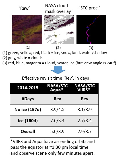
The investigation focuses on winter of 2014 and 2015, since they were amongst the coldest and longest since MODIS and VIIRS launched, and produced substantial ice cover within the study area. In total, 317 days were evaluated, ranging from Day 305 (1 November) in 2013 through Day 110 (20 April) in 2014 and from Day 311 (7 November) in 2014 through Day 91 (1 April) in 2015. The time ranges were selected to include those where ice presence could be inferred from the discharge data quality flag at the Harrisburg gauge (USGS01570500), plus an anterior and posterior buffer period of at least two weeks. While 2015 did not have any notable mid-winter thaws, a thaw period of about two weeks was noted within the 2014 time-range referred to as “ice” period. Visual inspection also showed that ice and snow are mostly concurrent, and thus time periods identified as “ice” also refer approximately to snow/ice cover periods.

On few occasions, data were either missing or otherwise not produced for the shortwave infrared (SWIR) bands used to develop the contrast-based cloud mask, and were treated as non-observations. Non-observations were also grouped together with cloudy data (overall referred to as cloudy), although in some instances the non-observed scene may have been cloud-free. This treatment is not considered to greatly impact any of the conclusions and presented results, since: (1) non-observations were rare; and (2) some of them would likely have been cloudy. For a time range spanning 317 days, MODIS-Terra, MODIS-Aqua and VIIRS, respectively, had seven (Day 345, 2013; Day 31, 2014; Day 73, 2014; Day 346, 2014; Day 50, 2015; Day 56, 2015; Day 63, 2015), one (Day 77, 2015) and two (Day 35, 2014; Day 316, 2014) non-observations.

3.2. MODIS/VIIRS Data

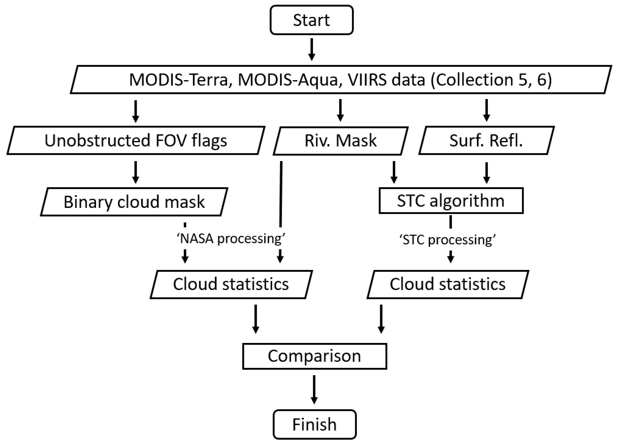
Data from MODIS collection 5 and 6 (MOD/MYD09GA) and VIIRS collection 3110 (NPP_DSRFLD _L2GD) for tile h12v04 were used, obtained from LAADS Web. Both products are similar in that they have surface reflectance data in the visible, near infrared and shortwave infrared bands gridded to 500 m on sinusoidal projection, are atmospherically corrected, include viewing geometry and respective cloud data on 1 km sinusoidal grids. MODIS data include two cloud masks, but only the “external” MOD35 mask was used. A binary cloud mask was derived from the unobstructed field-of-view (FOV) flags that are passed on from the MOD35 cloud products. In both cases, the products are composed of several observations that may have occurred during the day. We only took data from the first layer of the composited product. These data should be considered the best available observations according to the scoring/compositing scheme used [32].

3.3. Binary Cloud Mask for MODIS, VIIRS

The VIIRS (MODIS) cloud masks are categorized as confidently clear (clear), probably clear (not set), probably cloudy (mixed) and confidently cloudy (cloudy). A binary cloud mask was constructed by grouping “confidently clear” and “probably clear” as cloud-free and “probably cloudy” and “confidently cloudy” as clouds. To avoid alignment errors, coarser resolution cloud data were first sampled to 500 m grids via nearest neighbor interpolation, before further sub-setting to the region of study. The region of study consists of 158 by 154 grid cells (24,332 total).

3.4. Land-Water Mask

In order to ensure that identified grid cells mainly consist of water, it was also necessary to develop a land/water mask on 500 m resolution sinusoidal grid. This was accomplished from multispectral (bands 1–5 and 7) maximum likelihood classification of MYD09GA data. The classification was done on imagery from different times during low flows in summer and only those grid cells classified as water in every instance was kept. The process helps to limit sampling to mostly water only grids, and also ensures temporal stability in case of wandering river bed. We did not notice any significant changes in the river bed location during the investigated time periods (2001–2016). The final river mask consists of 402 grid cells, and was used to process all of MODIS and VIIRS data.

3.5. Parameters: Effective Revisit Time, Data, Absolute Cloud Cover

Cloud products and biases were evaluated using the metric “effective revisit time”, rev,

$$rev=\frac{d_{tot}}{data},$$

(1)

$$data=\frac{{{\displaystyle \sum }}_{n=0}^{n=d_{tot}}cf{g}_n}{402}$$

(2)

where d_tot is the number of samples (days), data is the average proportion of cloud free grids (cfg) within d_tot, 402 represents the total number of river grids within the field of view, cfg refers to the number of cloud-free grids (ranging from 0 to 402) on Day n. For example, if the river were fully free of clouds each day (data = d_tot), rev is equal to 1. If on average only half of the river is sampled every day (data = 0.5 × d_tot), rev becomes 2 days, and so forth. While it may be a stretch to refer to results based on analysis of only 317 days as a climatology, results are nonetheless expected to approximate the climatological mean.

Based on data presented in Section 2.2, a cloud cover estimate in terms of effective revisit time can be established. Assuming an absolute winter cloud cover of 75% for MODIS-Terra data yields rev = 4.0 days. Assuming a 5% higher absolute cloud cover of 80% for MODIS-Aqua data yields rev = 5.0 days. These approximate estimates correspond to the mean improvement of STC processing with NASA processing for Winter 2014: prior results, using slightly different cloud masking, yielded rev of 5.1 and 4.1 days, respectively, for NASA(Aqua) and STC(Aqua) [12]. We note that small differences in absolute cloud cover may have a disproportionate impact on effective revisit time: 5% can be the difference from rev = 1.05 to 1.0 days (no clouds), or that of rev = infinite to 20.0 days (100% vs. 95%). Since the base value is already high (~75%) in the region of study, small differences in absolute cloud cover are relevant.

3.6. Contrast-Based Cloud Mask Approach (STC)

The product cloud masks were also compared to cloudiness determined from STC [12]. The primary objective of STC is to detect the easier-to-identify the otherwise error-producing, opaque clouds: clouds which for the application of snow/ice monitoring obstruct the field of view to such a degree that it is not possible to accurately identify water, ice or snow. As indicated by the high occurrence of semitransparent single-layer clouds in the area (Section 2.2), more frequent, reasonably accurate observations may be realized. With respect to semitransparent clouds, it is difficult to ascertain whether a grid is exactly cloud-free or not, and whether a cloud mask truly produced a false detection: the cloud mask may have correctly detected an optically thin cloud, which in some cases may appear as “invisible” under visual inspection. In these cases, the view of the underlying surface is usually sufficiently clear to accurately classify whether there is water, ice/snow or bare land. We showed in previous work that STC(Aqua) vs. NASA(Aqua) outside of snow/ice cover provided similar effective revisit times (4.6 vs. 4.0 days), but performed substantially better during snow/ice cover (3.8 vs. 7.1 days), with no non-detections or false detections with respect to hydrometric station data. Further details on the algorithm and validation for MODIS-Aqua may be found in Kraatz et al. [12]. 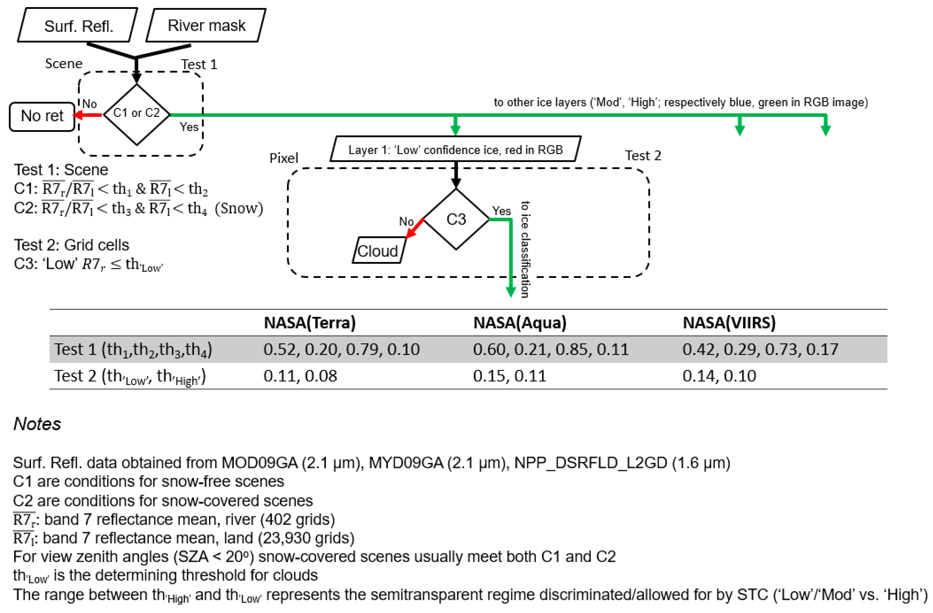The portion of the STC algorithm relevant to cloud screening, with information on the tests, conditions and thresholds is provided in Figure 3.

STC cloud discrimination consists of two test: Test 1 for evaluating the scene for optically thick clouds and if deemed reasonably cloud-free, individual grid cells are evaluated for clouds with Test 2. While the tests are intended to mainly detect view-obstructing opaque clouds, obstructing semitransparent clouds also tend to be routinely identified. Thresholds were derived from band statistics of land and water grid cells for each instrument, and thus are different for each platform. The thresholds for Test 1 were applied to the field of view reflectance mean of all land (river) grids, rather than individual grid cells. The obtained snow/cloud delineating thresholds correspond well with those found in literature. For band 7 (2.1 μm) a threshold of <0.1 was proposed by Dozier [22] and also adopted by Thompson et al. [11].

As part of Test 1, river and land grid cells need to be spectrally separable for snow-free (th₁) and snow-covered (th₃) scenes. Thresholds for snow-free scenes (th₁) requires stricter contrasting thresholds (ranging from 0.4 to 0.6) but allows for higher 1.6 μm (VIIRS) or 2.1 μm (MODIS) mean scene reflectance (th₂) compared to snow-covered scenes (th₄). Low view angle snow-covered scenes often meet both criteria of Test 1. If neither C1 nor C2 of Test 1 is met, the scene is not deemed of sufficient quality and not processed.

For cloud/ice discrimination of Test 2 for the low and moderate confidence layers, cloud delineating thresholds of 0.11, 0.15 (previously 0.19 in [12]) and 0.14 were used for MODIS-Terra, MODIS-Aqua and VIIRS, respectively. To be categorized as high confidence ice the SWIR bands are required to have values less than or equal to 0.08, 0.11 and 0.10 for MODIS-Terra, MODIS-Aqua and VIIRS, respectively. The range between the high and low thresholds represents the semitransparent range allowed (and discriminated) by the algorithm.

Due to how the algorithm is currently implemented, it is rarely possible that an apparently clear-sky, snow-covered scene may not be processed: while not necessarily deemed cloudy, there was not enough contrast to delineate snow-covered land from water/snow/ice grid cells in the band of choice. Overall, due to scenes not being selected by the algorithm at all if not passing Test 1, but being nonetheless partially sampled when cloud products are used, STC estimates of opaque clouds are expected to be somewhat conservative.

3.7. Validation Approach

The cloud-truth at any particular observation time of MODIS/VIIRS within the river reach is unknown. It is also not known a priori which of the cloud masks produces the closest approximation to cloud-truth. Cloud mask inter-comparisons would primarily yield information on their correspondence, rather than truth. While statistics based on rev can be informative and inform on obscuring cloud cover, its validity may be more solidly established via additional information. In this particular study cloud statistics are also linked to more readily verifiable data: that of ice cover maps [4,12]. We are able to evaluate whether STC cloud masking is credible not only by inference from cloud statistics from NASA and STC processing, but also from comparison of resulting ice cover maps to ice presence inferred from hydrometric station data. Unlike other available options, this method is practical and can be expected to provide a reasonable estimate of cloud-truth. Specific evaluations may be done on: (1) individual day basis by visual inspections of false color imagery; (2) ice extent time series for longer term evaluations; and (3) inferences based on effective revisit times.

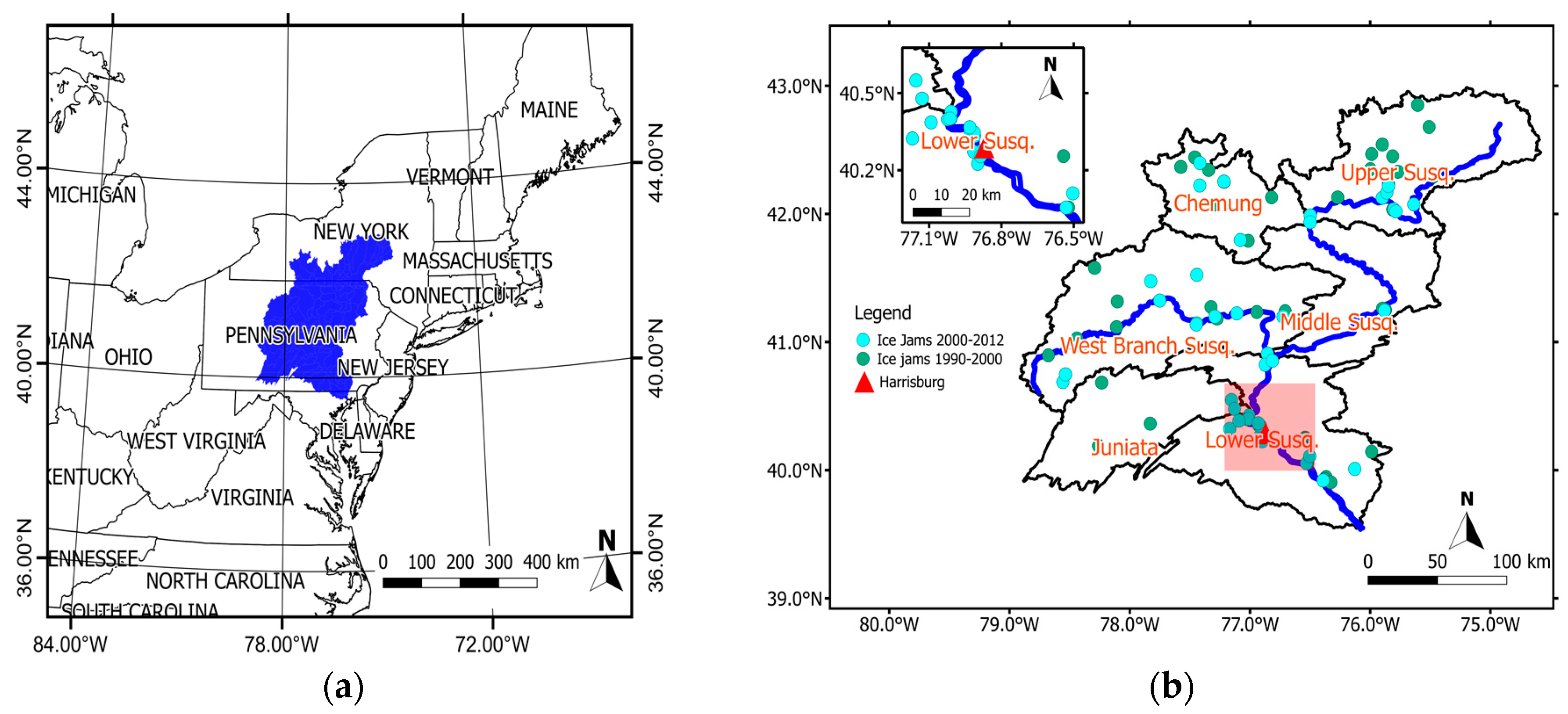
The hydrometric station (USGS 01570500) is located near the center of the field-of-view, at Harrisburg, PA. The station has a record of a daily discharge quality flag (DQF), and we previously showed that it can be reliably used to infer whether the portion of river within the FOV bears ice [12]. The discharge quality flag is set where it is not possible to accurately report discharge/stage within a given tolerance. Specifically, the DQF is set when the gauge malfunctions, or sufficient river ice is present such that it significantly impacts flow determinations. A look at discharge data for a >10-year period revealed that the flag is rarely raised outside of ice periods. Thus, it can be used to reliably inform on the presence of river ice. It is presumed unlikely that areal ice extent could consistently be related to the setting of the DQF, as it depends on the judgment of a Hydrologist. However, a reasonably strict estimate is that it would be set by when 10% river grids are ice covered (

Table 1. The validation criteria for the STC algorithm is a comparison of areal river ice extents obtained from satellite data processing to reach-wide ice cover inferred from a discharge data quality flag (DQF).

	DQF	STC, Ice Extent (% of Grids)
Non-detection (ice)	DQF set	<5
False detection (ice) or Non-detection (cloud, snow)	DQF not set	>10

).

The validation criteria presented in Table 1 allow for some inference with respect to the correct typing between cloud and cloud-free conditions, especially in instances where ice has not been observed or could not have formed due to warm temperatures. Missed opaque clouds, especially outside of ice cover periods, would be clearly represented by false ice detections. Generally, false ice detections are not solely attributable to missed clouds that were classified as ice. More problematic than missed clouds are false ice detections due to adjacent-to-river snow cover, when viewed at larger sensor zenith angle (SZA, e.g., more than 40 degrees). Besides footprint growth issues (more so for MODIS than VIIRS [28]), anisotropic scattering can also be problematic [15]. Both can combine to result in false positives, and from experience false positives due to snow occur more frequently and are more difficult to address using visible and SWIR bands only.

Using ice extent time series or cloud statistics within the field of view to ascertain whether clouds were missed is more difficult during ice/snow periods since: (1) STC is supposed to ignore some clouds, and estimate whether ice is underneath semitransparent clouds; and (2) not only missed clouds, but also adjacent snow cover may be classified as ice. However, by using three independently generated cloud statistics and ice time series, it is possible to ascertain more confidently about whether obscuring clouds are properly detected: significant ice cover overestimates due to e.g., missed clouds, or poor view geometry would be apparent between the three ice cover time series. Cloud errors would also be expected to show in the cloud statistic. However, using ice time series offers a clearer visual comparison.

4. Results

4.1. Cloud Statistics from NASA Processing

Results of NASA processing for 2014 and 2015 data are shown in

Table 2. Comparison of cloud mask statistics over river grid cells, categorized by ice cover, obtained from NASA processing. Data: see Equation (2); Obs: number of days on which at least one grid cell was observed; Rev: see Equation (1), in days. The number in brackets of the first column specifies how many days corresponded to “no ice” or “ice”, as per the discharge quality flag.

2014–2015	NASA(Aqua)			NASA(Terra)			NASA(VIIRS)
	Data	Obs	Rev	Data	Obs	Rev	Data	Obs	Rev
No ice (157 days)	40.1	78	3.9	40.4	82	3.9	50.5	105	3.1
Ice (160 days)	23.0	80	7.0	38.6	88	4.1	59.6	114	2.7
Totals (317 days)	63.1	158	5.0	79.0	170	4.0	110.1	219	2.9

. A break-down of 2014 and 2015 is not shown as results were similar. Table 2 data clearly shows that only NASA(Aqua) features a dramatically larger rev (7.0 vs. 3.9 days) the during snow/ice cover period. NASA(VIIRS) features a relatively smaller 2.7 vs. 3.1 days, while NASA(Terra) results remain nearly the same irrespective of snow/ice cover. NASA(Terra) and NASA(Aqua) revisit times outside of snow/ice periods are identical. NASA(VIIRS) has the by far lowest effective revisit times of 2.9 days compared to 4.0 and 5.0 for NASA(Terra) and NASA(Aqua), respectively. This is equivalent to 31 (40%) and 47 (75%) more full river observations (data) compared to NASA(Terra) and NASA(AQUA), respectively. Most of the difference stems from the 160 days considered “snow/ice” period: NASA(VIIRS) has 21 (54%) and 37 (160%) more full river observations (data) for NASA(Terra) and NASA(Aqua), respectively. We also note that NASA(VIIRS) has the most “Obs”, with 219 out of 317 scenes sampled from, versus 170 and 158 for NASA(Terra) and NASA(Aqua), respectively.

4.2. Cloud Statistics from STC Processing

Results of STC processing for 2014 and 2015 data are shown in

Table 3. Comparison of cloud mask statistics over river grid cells, categorized by ice cover, obtained from the STC algorithm. Data: see Equation (2); Obs: number of days on which at least one grid cell was observed; Rev: see Equation (1), in days. The number in brackets of the first column specifies how many days corresponded to “no ice” or “ice”, as per the discharge quality flag.

2014–2015	STC(Aqua)			STC(Terra)			STC(VIIRS)
	Data	Obs	Rev	Data	Obs	Rev	Data	Obs	Rev
No ice (157 days)	34.7	36	4.5	38.2	41	4.1	39.9	43	3.9
Ice (160 days)	47.4	48	3.4	37.3	38	4.3	46.8	49	3.4
Totals (317 days)	82.1	84	3.9	75.5	79	4.2	86.7	92	3.7

. A break-down of 2014 and 2015 is not shown as results were similar. Table 3 data show that the effective revisit times for STC(Aqua) and STC(VIIRS) are relatively decreased during “ice”: rev is 3.4 days, compared to 4.5 and 3.9 days during “no ice”, respectively. STC(Terra) has a slightly increased effective revisit time during “ice”, increased from 4.1 to 4.3 days. During “ice”, data obtained by STC(Aqua) and STC(VIIRS) are identical, corresponding to 47 full river observations. Overall, effective revisit times are similar: 4.2, 3.9 and 3.7 days, respectively, for STC(Terra), STC(Aqua) and STC(VIIRS). STC(Terra), STC(Aqua) and STC (VIIRS), respectively, fully observe the river 76, 82 and 87 times within the 317 days. Data sampling (“Obs”) is also similar with river observations stemming from 79, 84 and 92 selected scenes, respectively, for STC(Terra), STC(Aqua) and STC(VIIRS). This corresponds to an overall mean sampling rate of 96% of river grids when a scene is selected for processing by STC.

Image selection of STC processing is compared to that of NASA in

Table 4. Shown are the proportion of river grids sampled as clear-sky by NASA processing when STC accepts (few clouds) or rejects (cloudy) a scene for 2014 and 2015. Data: see Equation (2); #: number of days sampled/rejected by CRIOS-STC; Ret: Average cloud-free river grids (Data/#).

Collection 5	2014						2015
	STC Samples			STC Rejects			STC Samples			STC Rejects
	Data	#	Ret	Data	#	Ret	Data	#	Ret	Data	#	Ret
NASA(Terra)	32.8	45	73%	12.9	126	10%	24.8	34	73%	8.5	112	8%
NASA(Aqua)	24.6	44	56%	8.8	127	7%	22.5	40	56%	7.3	106	7%
NASA(VIIRS)	41.5	49	85%	18.9	122	15%	36.4	43	85%	15.3	103	15%

: A breakdown by year is shown, detailing how much data are obtained from NASA processing when STC accepts or rejects a scene. The data provided in Table 4 indicate nearly identical results between 2014 and 2015 data. It shows that NASA(Terra), NASA(Aqua) and NASA(VIIRS), respectively, indicate that 73%, 56% and 85% of river grids are cloud free in scenes accepted by STC and that 9%, 7% and 15% of river grids are cloud free in scenes rejected by STC.

Provided that STC processing overall samples 96% of river grids as cloud free, it samples 23%, 40% and 11% more data from imagery than NASA(Terra), NASA(Aqua) and NASA(VIIRS).

4.3. Ice/Cloud Results from STC Processing

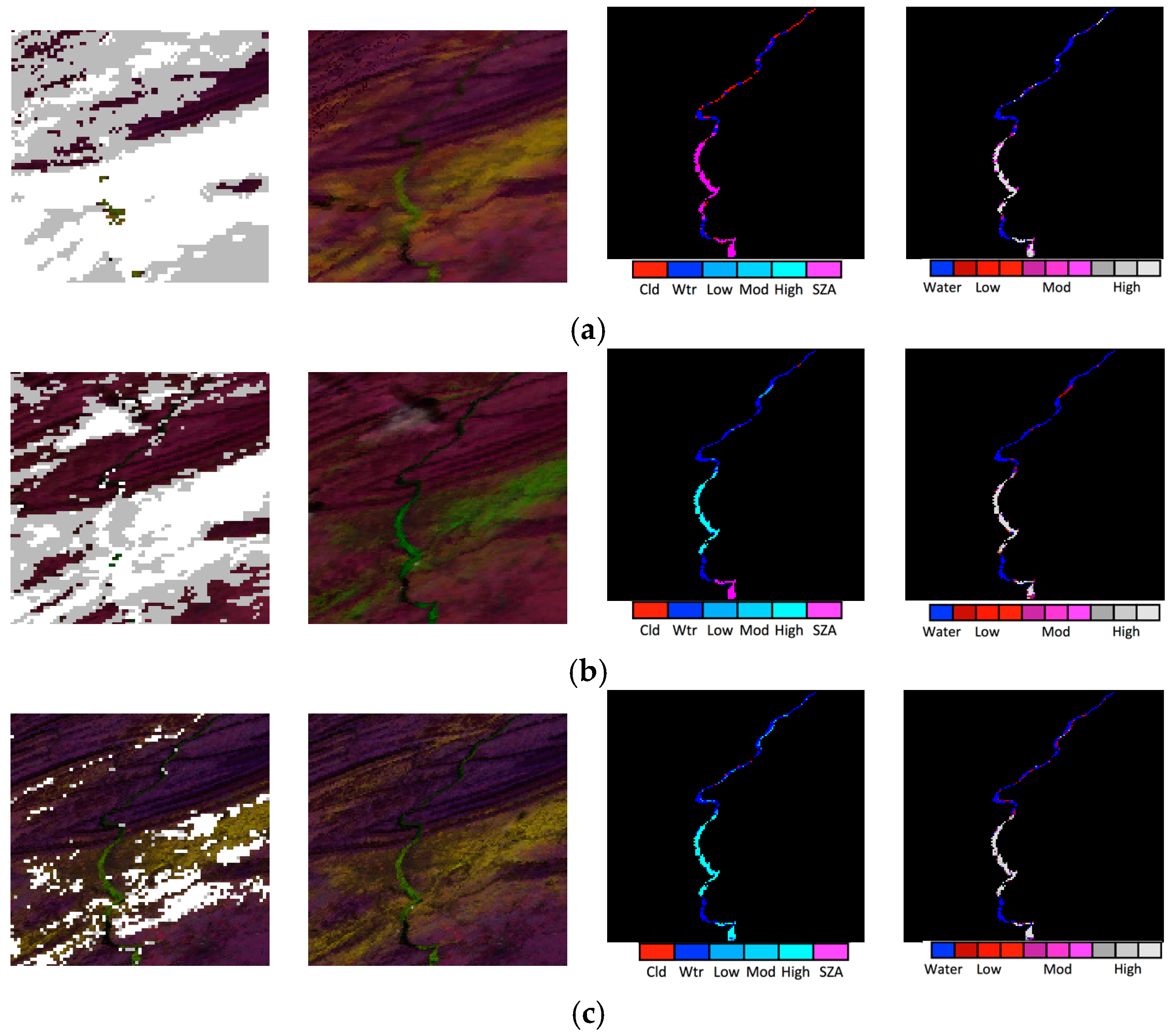
An example of STC processing of data for clouds and ice is provided in Figure 4. The example is for an ongoing ice jam, as identified per the National Weather Service, on 9 January 2014.

The leftmost column shows an overlay of NASA cloud processing results on top of false color imagery. MODIS data are cloudier than VIIRS data. The second column from the left provides the false color imagery, showing that river (black), ice (yellow-green), snow (yellow-green) and land (magenta) can be reasonably well identified by visual inspection. The third column is the main product from which the time series and cloud statistics are developed, and shows the result of STC processing: ice vs. cloud confidence in three levels (“Low”, “Mod”, and “High”), a warning flag for large sensor zenith angle (SZA, >40°, only marked at “ice” grids), water and clouds. Terra data were obtained at poor SZA, and as result STC classified some river grids as clouds in the upper portion of the river. The fourth column shows the running composite. It is only shown here to more clearly indicate the ice/cloud confidence levels, which are further subset according to reflectance magnitude, since the running composite maps do not overlay information on clouds or SZA. The figure shows the cloud-clearing ability of STC vs. NASA processing. All classified ice maps are in good agreement with visual inspection. Ice/water delineations are nearly identical. Ice is classified with similar confidence between the platforms.

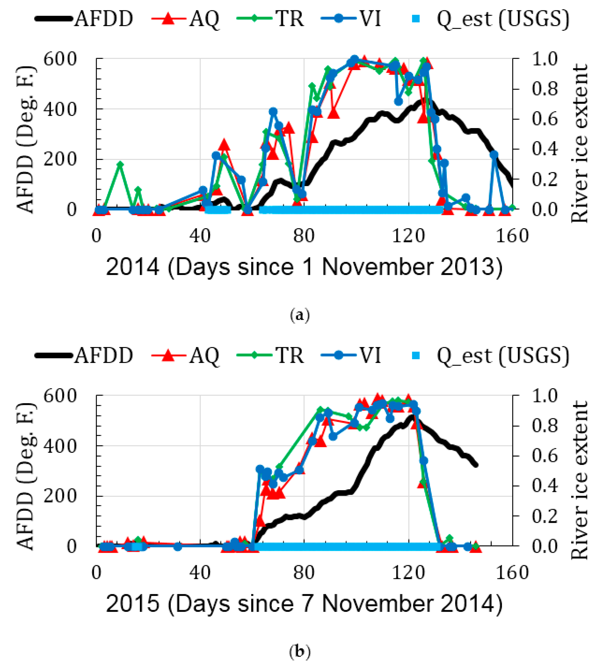
Figure 5 shows the river ice time series for 2014 and 2015, indicating that: (1) ice detection is consistent with that inferred from the hydrometric station; and (2) generally, similar results are obtained irrespective of platform or bands used. Based on the consistency of ice extent time series, a high correlation is evident. The correlations of “ice extent” for the different platform combinations were computed based on >50 common observations from STC for each possible combination and range from 95%–99%. Mean absolute differences of ice extent based on these common observations range from 3%–7%. The accumulated freezing degree-day (AFDD) curve is provided only for contextual, qualitative information regarding whether freezing or thawing air-temperatures persist: it should be interpreted here only in terms of that its increase (decrease) represents below-zero (above-zero) temperatures [12,33,34].

Table 5. Shown are summary error statistics for the 2014–2015, relating to reach-wide ice detection vs. that inferred from hydrometric station data: probability of ice detection (POD), proportion correct (PC), false detection (FD) and non-detection (ND).

	POD (%)	PC (%)	FD (%)	ND (%)
STC(Terra)	95	97	3	0
STC(Aqua)	100	100	0	0
STC(VIIRS)	92	95	4	1

shows the reach-wide ice detection error metrics, for probability of detection of ice (POD), proportion correct (PC), false detections (FD) and non-detections (ND)—after filtering out a gauge malfunction (2015, Days 15 and 16) since it could not be reasonably used as indicator of ice: it was too early in the season and temperatures were too warm, as evident from the AFDD curve. Error metrics indicate good performance overall, with 95%–100% proportion correct.

4.4. On Collection 5 vs. Collection 6 Differences

Collection 6 (C6) NASA(MODIS) features a higher resolution land/water mask (250 m vs. 1 km in C5). Although NASA(MODIS) does not feature a dedicated inland water processing path, the new land/water mask may still lead to improved cloud masking over river grids. For this reason, and to generally assess how STC and NASA processing are impacted by re-processed data, we include a brief comparison between C5 and C6. Results of a direct comparison of NASA(Aqua) data are provided in

Table 6. Comparison of NASA(Aqua) C5 to C6 reprocessing, on river grids cells only. Data: see Equation (2); Obs: number of days on which at least one grid cell was observed; Rev: see Equation (1), in days.

2014–2015	NASA(Aqua), C5			NASA(Aqua), C6
	Data	Obs	Rev	Data	Obs	Rev
No ice (157 days)	40.1	78	3.9	39.9	78	3.9
Ice (160 days)	23.0	80	7.0	23.2	84	6.9
Totals (317 days)	63.1	158	5.0	63.1	162	5.0

and show that there are few, if any, differences between C6 and C5 data with respect to cloud masking over river. On average for MODIS (Terra and Aqua) data, only 10 grids per day (2% of river grids) changed between cloudy and clear. Differences amount to one (zero) fewer full river observations over the 317 days for MODIS-Terra (MODIS-Aqua). Differences in excess of 30% were noted on four occasions, three of which trended towards fewer clear-sky river grids.

Impacts of Collection 6 data on STC were also investigated, but, due to small differences, are not detailed here. The contrast based algorithm is not sensitive to differences between C5 and C6 processing: only on three occasions (one for MODIS-Terra, two for MODIS-Aqua) did the slightly different reflectance magnitudes result in selection (one) or rejection (two) of originally near-threshold scenes. Outside of these scenes, only 0.1 out of the 402 river grids/scene was classified differently in light of collection 6 data. Overall, we find that C5 and C6 data are virtually identical to each other over river grids thus C5 and C6 data may be used interchangeably, and that conclusions drawn from investigation of either should be applicable to both.

5. Discussion

Cloud statistics obtained from NASA processing clearly indicate that there are significant differences with respect to cloud identification. Considering the differences between detector capabilities, algorithm and ancillary data sources used for cloud masking, differences are to be expected. Most relevant to river ice monitoring is that (1) NASA(Aqua) appears to strongly overestimate clouds during snow/ice presence, (2) NASA(MODIS) regularly may identify apparently cloud-free river ice as clouds and (3) NASA(VIIRS) indicates substantially fewer clouds than NASA(MODIS).

5.1. NASA(MODIS) Snow/Ice Underdetections

Attribution is difficult, especially in light of the focus of this work which is an evaluation of an alternate approach to better observe river ice. We point to some of the differences noted in using band 7 (2.1 μm) NDSI, namely that (a) it provides results of up to 5% larger snow extent; (b) the NDSI threshold for snow is substantially larger for NASA(Aqua) than NASA(Terra) (>0.54 vs. >0.40); (c) that the Normalized Difference Vegetation Index (NDVI) portion of the snow decision region has been disabled for NASA(Aqua) due to snow errors and (d) that differences are more apparent in low illumination and dense forests. The NDVI portion of the snow decision region is used to improve snow classification underneath canopies, and this consideration allows for lower-than NDSI threshold data to also be classified as snow.

Most likely, the difference stems from use of a globally calibrated threshold that is not ideal for this region, nor ice detection. Based on the thresholds presented in this and prior work, we can provide an illustrative sample calculation. Our own threshold for snow detection was found to correctly identify 21 out of 22 scenes as having snow and used values of 0.1 for band 7. We further note that a fully snow covered, cloud-free scene may have a mean reflectance as low as 0.05—the point at which contrast-based approach can fail. The values of 0.1 (0.05) may be substituted into the NDSI test, to solve for the required magnitude of visible reflectance. The result yields a required band 4 (0.55 μm) reflectance of at least 0.34 (0.17). Noting that band 7 reflectance over snow covered land is usually much closer to 0.1 than 0.05 in our histograms and that many (including snow covered) land grids may not have a band 4 reflectance in excess of 0.34 (Figure 6 in [12]), it is not surprising that the band 7 based NDSI test may fail in this setting and that snow and ice can instead be identified as clouds. It is important to note that the NDSI tests use at-satellite reflectance data, which are different from our dataset because the latter underwent additional processing via an atmospheric correction algorithm [35].

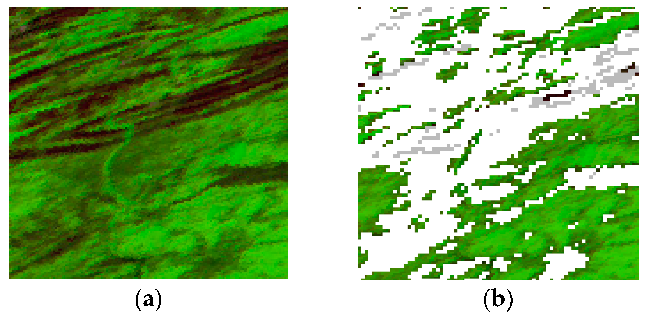
A representative example is provided in Figure 6, showing a snow covered scene. Even under full snow cover, multiple darker appearing features are apparent. More easily identified are those due to terrain (hills, ridges). Less obvious are those patches near the center of the field of view, where river ice is also usually found (Figure 6a). These patches are consistent with snow masked by vegetation (or other) canopy or frozen water. The cloud mask overlay (Figure 6b) shows that the relatively darker patches tend to be identified as clouds, while the brightest grids are “clear”. This is consistent with the general sample computation, indicating that the threshold for NDSI may not be readily met in the vicinity of where river ice is found. It also is not helpful that NASA(Aqua) does not allow for a potentially lower NDSI threshold on basis of vegetation masking of snow, as its NDSI/NDVI decision region is disabled. A second factor is that snow-free or water-ice mixtures tend to have a significantly smaller band 4 reflectance than snow.

With respect to river ice being detected as clouds, we note that ice cover may occur without substantial snow cover. When determining a processing path, NASA(MODIS) refers to the background flag, set by a coarse resolution product (25 km by 25 km). If the grid is only partially snow covered the flag may not be set as snow, no NDSI test is done, and high reflectance grids would be classified as clouds [11].

5.2. NASA(VIIRS) Bias

We find that NASA(VIIRS) detects substantially fewer clouds than NASA(MODIS). Key et al. [28] provide some information on NASA(VIIRS), but their results are reported on basis of only sampling data from “confidently clear” grids. They note substantial errors due to extensive cloud misses and snow overestimates when data are sampled from “probably clear” and “probably cloudy” grids. Even with the strictest cloud mask they noted obvious cloud misses occurring in the midst of large cloud masses, resulting in snow overestimates.

Our own observations and data corroborate the observations made by Key et al. [28]. Our results (Table 4) show that NASA(VIIRS) samples exceedingly from scenes rejected by STC processing—at about twice the rate than NASA(MODIS). STC(VIIRS) selects 92 out of 317 days for processing. At a sampling rate of 15% from rejected scenes, there would be nearly 34 additional full river observations, whereas NASA(Terra) and NASA(VIIRS) would only obtain 19 and 16, respectively. NASA(VIIRS) tendency to sample data from cloudy scenes is also apparent from its high value for “Obs” (Table 3): NASA(VIIRS) samples the river on 30%–40% more days compared to NASA(MODIS). Correspondingly, NASA(VIIRS) also has almost proportionally more data (~40% compared to NASA(Terra)).

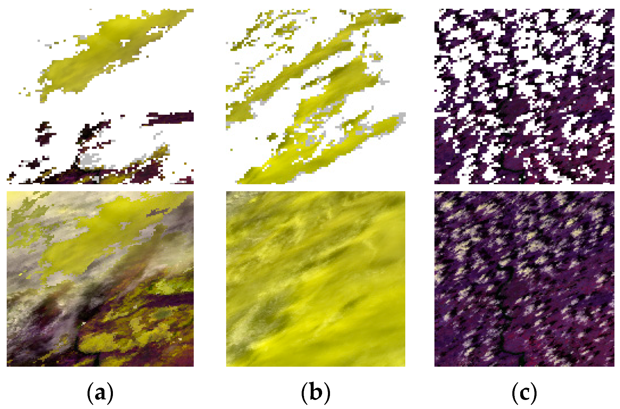
The remaining factor providing NASA(VIIRS) with a lower effective revisit time can be attributed to it identifying 12% and 29% more river grids as clear-sky (STC accepted scenes), compared to NASA(Terra) and NASA(Aqua) (Table 4). Figure 7 presents qualitative examples on how NASA(VIIRS) obtains additional river observations where NASA(MODIS) or STC processing would not allow for a substantial amount of river data to be sampled.

5.3. Diurnal Cloud Cover Discrepancy

NASA processing provided inconclusive data on whether there are fewer clouds in the morning or afternoon. According to Ackerman et al. [31], NASA(Aqua) appears to observe 5% more clouds than NASA(Terra). Our results in Table 2 also indicate a 5% mean absolute cloud cover difference corresponding to the difference in “rev” for NASA(Terra) (4.0 days, 0.75 absolute cloud cover) versus NASA(Aqua) (rev = 5.0 days, 0.80 absolute cloud cover). However, NASA(VIIRS) data suggested a much smaller absolute cloud cover of 0.65, but as shown in Section 5.2. NASA(VIIRS) does not provide reliable information. The reference provided by STC processing suggests that afternoon observations may have 2%–3% less absolute cloud cover. Much of the overall difference stems from the “ice” period, during which afternoon observations suggest an absolute cloud cover of only 0.71 compared to 0.77 for STC(Terra). The precise reason for this difference, mainly occurring only during snow/ice cover period, is unclear. Although STC(VIIRS) uses the 1.6 μm band instead of 2.1 μm for STC (MODIS), both STC(VIIRS) and STC(Aqua) indicate the same. Concluding, it is more likely than not that afternoons are slightly less cloud obstructed, contradicting results obtained from NASA processing.

5.4. Suitability of NASA Processing for River Ice Mapping

Each of the NASA processing was shown to yield substantially different results. NASA(Aqua) is clearly the least well suited for river ice monitoring, as it most frequently identifies ice as clouds, and only samples 56% (Table 4) of river grids in mostly clear scenes. On basis of results in Table 2 and Table 3, NASA(Terra) statistics approximate that of STC more closely than NASA(VIIRS). However, since NASA(MODIS) has a general and somewhat persistent tendency to identify ice as clouds, it is less suitable than indicated by cloud statistics alone: although, on average it may sample 73% of river grids, it may mask the data being sought. NASA(VIIRS) provides the smallest effective revisit times, but we were able to show that much of it is due to clouds that were not identified by NASA(VIIRS). STC(VIIRS) provides good ice and cloud identification (Figure 2 and Figure 3, Table 5), and its results suggest that its effective revisit time should be closer to 3.7 days (0.73 absolute cloud cover) than 2.9 days (0.65 absolute cloud cover) for NASA(VIIRS). Nonetheless, when STC accepted a scene for processing, NASA(VIIRS) sampling most closely approximated STC results: not only because it sampled 85% of the river compared to 96% for STC, but also because there were no obvious, systematic misidentifications of ice as clouds. Owing to these properties NASA(VIIRS) is more suitable for river ice monitoring than NASA(MODIS), but care should to be taken to screen for undetected clouds. These would be more difficult to notice within an ice product while the river already bears ice: it may appear as correctly identified ice, surrounded by clouds (e.g., Figure 7a,b)—although all data should have been classified as cloud.

5.5. Improved River Ice Mapping through Improved Cloud Masking

Figure 2 and Figure 3 and Table 3, Table 4 and Table 5 establish the capabilities of STC processing, that its results are credible and that it is more likely to approximate a cloud truth than any of the NASA processing. Table 3 details that STC processing provided consistent cloud identification across several platforms. Table 4 shows that STC is consistent with the NASA processing results: the fact that STC identified cloud-free scenes correctly is generally corroborated by the fact that 56% (NASA(Aqua)), 73% (NASA(Terra)) and 85% (NASA(VIIRS)) of river grids were also “clear”. Scenes identified as cloudy by STC were likewise generally identified as cloudy by NASA processing. Visual inspection of Figure 4 shows that ice cover is similarly and accurately identified, irrespective of platform or bands used. Thus, through consistency of data and low error rates (Table 3, Table 4 and Table 5), we infer that obstructing clouds must have been accurately identified by STC.

The overall expected effective revisit time appears to be near 4 days for each instrument. While this is approximately comparable to NASA(MODIS), worse than NASA(VIIIRS) and better than NASA(Aqua), the resulting data provide more reliable information and are quality checked. Furthermore, STC processing during “ice” has an effective revisit time of up to 3.4 days. Ice maps are readily composited between the platforms, allowing for a more continuous data record via cloud-clearing by using data obtained at different times or in more favorable physical settings (e.g., better view geometry). Specifically, in Table 3 for STC processing total “Obs” are listed respectively as 84, 79 and 92 for NASA(Aqua), NASA(Terra) and NASA(VIIRS). However, 116 individual days were selected for processing by STC between them. At 96% grids sampled in each of 116 days, out of 317, it is possible to achieve an effective revisit time of 2.8 days. Likewise, it is possible to further reduce errors by substituting the most accurate ice map of either platform. For the investigated time range it is possible to remove two false detections in STC(Terra) and STC(VIIRS) by substitution of STC(Aqua) data for those days. One non-detection for STC(VIIRS) can also be removed by substitution of STC(Terra) data.

6. Conclusions

The main goal of this work was to elucidate on cloud mask performance and suitability over ice-bearing rivers and on improving river ice observations. The goal was accomplished via a series of steps. First, cloud statistics based on binary cloud masks developed from the unobstructed field of view flags from the Moderate Resolution Imaging Spectroradiometer (MODIS) and the Visible Infrared Imaging Radiometer Suite (VIIRS) cloud products (MOD35, MYD35 and VCM) were developed. In all cases, data were sampled only from “confidently clear” and “probably clear” grids. Results show a large possible range for absolute cloud cover while ice and snow are found: 0.63, 0.76 and 0.84, respectively, for NASA(VIIRS), NASA(Terra) and NASA(Aqua). These cloud amounts correspond to one full river observation every 2.7, 4.1 and 7.0 days (effective revisit time), during the ice cover period. We showed that, when data are averaged, these difference become less apparent for MODIS, and obtained effective revisit times matching a 0.05 absolute cloud difference extrapolated from Ackerman et al. [31].

A contrast-based algorithm (STC) operating on MODIS and VIIRS surface reflectance data was used to provide reference cloud statistics. The validity of STC results are established on basis of: (1) providing accurate ice detection relative to that inferred from an in-situ, reach-representing, discharge quality flag; and (2) consistency of cloud statistics and resulting river ice time series to show STC has few, if any, serious cloud detection errors. Cloud statistics obtained from STC processing provided more consistent absolute cloud cover values while ice and snow are found: 0.71, 0.77 and 0.71 for STC (VIIRS), STC(Terra) and STC(Aqua) data, respectively. STC processing suggests that afternoon data are obtained under less cloudy conditions: MODIS-Aqua and the VIIRS data suggested absolute cloud amounts of 0.74 and 0.73 overall, compared to the MODIS-Terra value of 0.76. This conclusion contradicts results obtained from the original MODIS cloud masks, which indicated that the afternoon has 0.05 greater absolute cloud coverage.

We also provided insight and attribution into the reasons for various cloud biases. Our qualitative analysis suggests that differences between NASA(Aqua) and NASA(Terra) is probably due to the modified Normalized Difference Snow Index (NDSI) test that NASA(Aqua) uses. In addition, NDSI test may be more likely to fail for ice or ice/water mixed grids owing to relatively smaller 0.55 μm reflectance compared to snow. As result, these locations would be more frequently mapped as clouds. We also noted a tendency of both MODIS instruments to misidentify ice as clouds, especially when there is no or only partial snow cover, probably due to a scale-related inaccuracy [11]. The substantially smaller absolute cloud cover determined from NASA(VIIRS) was attributed to: (1) its identification of optically thick clouds as “clear” data; and (2) it generally sampling more data from apparently clear scenes as established from both visual inspection and STC processing. Differences and impacts of using Collection 6 (C6) vs. Collection 5 (C5) data in NASA and STC processing were also investigated. Although C6 features various algorithm tweaks and an improved land/water mask, we find that there are no significant differences for river monitoring, and conclude that C6 and C5 data may be used interchangeably.

We also noted how the improved cloud screening (e.g., that provided from STC) may lead to greatly improved river ice mapping capabilities. The improvement is mainly due the additional quality controls providing more reliable data than provided by NASA processing, and reduction of biases present in all of the NASA processing. Furthermore, during ice periods, STC provides lower revisit times than all but NASA(VIIRS) processing. Since the ice and cloud mapping is consistent and done over an identical river mask, the ice maps may be used interchangeably. We show that such cross-platform compositing would allow for an improved effective revisit time of up to 2.8 days. With cross-platform compositing it is also possible to further improve data quality by building ice cover time series based on the best quality observations.

Beyond its utility to river ice monitoring, ice data generated by this approach may be a useful input for ice jam modeling. Statistical modeling approaches have been mainly limited to using AFDD (and its few day difference) and discharge to model river ice dynamics such as break-up or freeze-up timing [36,37,38]. With ice data (reflectance as proxy) in addition to AFDD (air temperatures as proxy), it may be possible to build better models. MODIS has been operational since 2000 and a more complete series of river observations may lead to more accurate determination of break-up timing, freeze-up or other work related to river ice processes and climatology [18,39].

Likewise, it would be of interest to explore the cloud clearing potential of GOES-R, with respect to river ice observations. The GOES-R Advanced Baseline Imager (ABI) is compatible with the STC approach, as it features an appropriate shortwave infrared and 500 m resolution visible band. GOES-R should provide excellent river ice monitoring capability for this stretch of the Susquehanna River.

References

1. Vorosmarty, C.; Askew, A.; Grabs, W.; Barry, R.G.; Birkett, C.; Doll, P.; Goodison, B.; Hall, A.; Jenne, R.; Kitaev, L.; et al. Global water data: A newly endangered species. Eos Trans. Am. Geophys. Union 2001, 82, 54–58. [Google Scholar] [CrossRef]
2. Fekete, B.M.; Robarts, R.D.; Kumagai, M.; Nachtnebel, H.-P.; Odada, E.; Zhulidov, A.V. Time for in situ renaissance. Science 2015, 349, 685–686. [Google Scholar] [CrossRef] [PubMed]
3. Li, S.; Sun, D.; Yu, Y.; Csiszar, I.; Stefanidis, A.; Goldberg, M.D. A new short-wave infrared (SWIR) method for quantitative water fraction derivation and evaluation with EOS/MODIS and landsat/TM data. IEEE Trans. Geosci. Remote Sens. 2013, 51, 1852–1862. [Google Scholar] [CrossRef]
4. Chaouch, N.; Temimi, M.; Romanov, P.; Cabrera, R.; McKillop, G.; Khanbilvardi, R. An automated algorithm for river ice monitoring over the Susquehanna River using the MODIS data. Hydrol. Process. 2012, 28, 62–73. [Google Scholar] [CrossRef]
5. Ackerman, S.A.; Strabala, K.I.; Menzel, W.P.; Frey, R.A.; Moeller, C.C.; Gumley, L.E. Discriminating clear sky from clouds with MODIS. J. Geophys. Res. 1998, 103, 32–141. [Google Scholar] [CrossRef]
6. Riggs, G.A.; Hall, D.K. Reduction of cloud obscuration in the MODIS snow data product. In Proceedings of the 59th Eastern Snow Conference, Stowe VT, USA, 6 June 2002; Volume 5.
7. Strabala, K.I. MODIS Cloud Mask User’s Guide; University of Wisconsin–Madison: Madison, WI, USA, 2005. [Google Scholar]
8. Baker, N. VCM ATBD: VIIRS Cloud Mask Algorithm Theoretical Basis Document: 474-00033 (Rev E); Goddard Space Flight Center: Greenbelt, MD, USA, 2014. [Google Scholar]
9. Sirguey, P.; Mathieu, R.; Arnaud, Y. Subpixel monitoring of the seasonal snow cover with MODIS at 250 m spatial resolution in the Southern Alps of New Zealand: Methodology and accuracy assessment. Remote Sens. Environ. 2009, 113, 160–181. [Google Scholar] [CrossRef]
10. Hall, D.K.; Riggs, G.A. Accuracy assessment of the MODIS snow products. Hydrol. Process. 2007, 21, 1534–1547. [Google Scholar] [CrossRef]
11. Thompson, J.A.; Paull, D.J.; Lees, B.G. An improved liberal cloud-mask for addressing snow/cloud confusion with MODIS. Photogramm. Eng. Remote Sens. 2015, 81, 119–129. [Google Scholar]
12. Kraatz, S.; Khanbilvardi, R.; Romanov, P. River ice monitoring with MODIS: Application over Lower Susquehanna River. Cold Reg. Sci. Technol. 2016, 131, 116–128. [Google Scholar] [CrossRef]
13. Riggs, G.; Hall, D.K. Snow mapping with the MODIS Aqua instrument. In Proceedings of the 61st Eastern Snow Conference, Portland, ME, USA, 10 June 2004; pp. 9–11.
14. Maddux, B.C.; Ackerman, S.A.; Platnick, S. Viewing geometry dependencies in MODIS cloud products. J. Atmos. Ocean. Technol. 2010, 27, 1519–1528. [Google Scholar] [CrossRef]
15. Warren, S.G.; Brandt, R.E.; O’Rawe Hinton, P. Effect of surface roughness on bidirectional reflectance of Antarctic snow. J. Geophys. Res. Planets 1998, 103, 25789–25807. [Google Scholar] [CrossRef]
16. Wilson, A.M.; Parmentier, B.; Jetz, W. Systematic land cover bias in Collection 5 MODIS cloud mask and derived products—A global overview. Remote Sens. Environ. 2014, 141, 149–154. [Google Scholar] [CrossRef]
17. Carroll, M.L.; Townshend, J.R.; DiMiceli, C.M.; Noojipady, P.; Sohlberg, R.A. A new global raster water mask at 250 m resolution. Int. J. Digit. Earth 2009, 2, 291–308. [Google Scholar] [CrossRef]
18. Muhammad, P.; Duguay, C.; Kang, K.K. Monitoring ice break-up on the Mackenzie River using MODIS data. Cryosphere 2016, 10, 569. [Google Scholar] [CrossRef]
19. Godin, R. Joint Polar Satellite System (JPSS) Operational Algorithm Description (OAD) Document for VIIRS Cloud Mask (VCM) Intermediate Product (IP) Software; Goddard Space Flight Center: Greenbelt, MD, USA, 2015. [Google Scholar]
20. Riggs, G.A.; Hall, D.K.; Salomonson, V.V. A snow index for the Landsat thematic mapper and moderate resolution imaging spectroradiometer. In Proceedings of the IEEE International Geoscience and Remote Sensing Symposium—Surface and Atmospheric Remote Sensing: Technologies, Data Analysis and Interpretation, Piscataway, NJ, USA, 8–12 August 1994; Volume 4, pp. 1942–1944.
21. Klein, A.G.; Hall, D.K.; Riggs, G.A. Improving snow cover mapping in forests through the use of a canopy reflectance model. Hydrol. Process. 1998, 12, 1723–1744. [Google Scholar] [CrossRef]
22. Dozier, J. Spectral signature of alpine snow cover from the Landsat Thematic Mapper. Remote Sens. Environ. 1989, 28, 9–22. [Google Scholar] [CrossRef]
23. Warren, S.G. Optical Properties of Snow. Rev. Geophys. 1982, 20, 67–89. [Google Scholar] [CrossRef]
24. Gladkova, I.; Grossberg, M.; Bonev, G.; Romanov, P.; Shahriar, F. Increasing the Accuracy of MODIS/Aqua Snow Product Using Quantitative Image Restoration Technique. IEEE Geosci. Remote Sens. Lett. 2012, 9, 740–743. [Google Scholar] [CrossRef]
25. Gladkova, I.; Shahriar, F.; Grossberg, M.; Frey, R.A.; Menzel, W.P. Impact of the Aqua MODIS Band 6 Restoration on Cloud/Snow Discrimination. J. Atmos. Ocean. Technol. 2013, 30, 2712–2719. [Google Scholar] [CrossRef]
26. Wang, L.; Qu, J.J.; Xiong, X.; Hao, X.; Xie, Y.; Che, N. A new method for retrieving band 6 of Aqua MODIS. IEEE Geosci. Remote Sens. Lett. 2006, 3, 267–270. [Google Scholar] [CrossRef]
27. Li, X.; Shen, H.; Zeng, C.; Wu, P. Restoring Aqua MODIS band 6 by other spectral bands using compressed sensing theory. In Proceedings of the 2012 4th Workshop on Hyperspectral Image and Signal Processing: Evolution in Remote Sensing, Shanghai, China, 4–7 June 2012; pp. 1–4.
28. Key, J.R.; Mahoney, R.; Liu, Y.; Romanov, P.; Tschudi, M.; Appel, I.; Maslanik, J.; Baldwin, D.; Wang, X.; Meade, P. Snow and ice products from Suomi NPP VIIRS. J. Geophys. Res. Atmos. 2013, 118, 12816–12830. [Google Scholar] [CrossRef]
29. Duveiller, G.; Baret, F.; Defourny, P. Crop specific green area index retrieval from MODIS data at regional scale by controlling pixel-target adequacy. Remote Sens. Environ. 2011, 115, 2686–2701. [Google Scholar] [CrossRef]
30. Wynne, T.T.; Stumpf, R.P.; Tomlinson, M.C.; Dyble, J. Characterizing a cyanobacterial bloom in western Lake Erie using satellite imagery and meteorological data. Limnol. Oceanogr. 2010, 55, 2025–2036. [Google Scholar] [CrossRef] [Green Version]
31. Ackerman, S.A.; Holz, R.E.; Frey, R.; Eloranta, E.W.; Maddux, B.C.; McGill, M. Cloud detection with MODIS. Part II: Validation. J. Atmos. Ocean. Technol. 2008, 25, 1073–1086. [Google Scholar] [CrossRef]
32. Vermote, E.F.; Kotchenova, S.Y.; Ray, J.P. MODIS Surface Reflectance User’s Guide; MODIS Land Surface Reflectance Science Computing Facility: Greenbelt, MD, USA, 2011. [Google Scholar]
33. Stefan, J. Über die Theorie der Eisbildung, insbesondere über die Eisbildung im Polarmeere. Ann. Phys. 1891, 278, 269–286. [Google Scholar] [CrossRef]
34. Zubov, N.N. Arctic Ice; Air Force Geophysics Lab: Hanscom AFB, MA, USA, 1979. [Google Scholar]
35. Vermote, E.F.; Vermeulen, A. Atmospheric Correction Algorithm: Spectral Reflectances (MOD09); ATBD Version 4.0; University of Maryland: College Park, MD, USA, 1999. [Google Scholar]
36. Mahabir, C.; Hicks, F.; Fayek, A.R. Neuro-fuzzy river ice breakup forecasting system. Cold Reg. Sci. Technol. 2006, 46, 100–112. [Google Scholar] [CrossRef]
37. Tao, W.; Kailin, Y.; Yongxin, G. Application of artificial neural networks to forecasting ice conditions of the Yellow River in the Inner Mongolia Reach. J. Hydrol. Eng. 2008, 13, 811–816. [Google Scholar] [CrossRef]
38. Massie, D.D.; White, K.D.; Daly, S.F. Application of neural networks to predict ice jam occurrence. Cold Reg. Sci. Technol. 2002, 35, 115–122. [Google Scholar] [CrossRef]
39. Cooley, S.W.; Pavelsky, T.M. Spatial and temporal patterns in Arctic river ice breakup revealed by automated ice detection from MODIS imagery. Remote Sens. Environ. 2016, 175, 310–322. [Google Scholar] [CrossRef]
Figure 1. Overview of the approach used, detailing data and processes used to obtain the cloud statistics for NASA and STC processing. FOV stands for field-of-view.
Remotesensing 09 00229 g001
Figure 2. (a) The general location of the Susquehanna River basin (blue); and (b) its sub-basins (black), major river branches (blue) and locations of past ice jams (teal) obtained from the Ice Jam Database (Available at http://icejams.crrel.usace.army.mil/). The region of study is indicated by the map inset, and is approximately centered at Harrisburg, PA, USA.
Remotesensing 09 00229 g002
Figure 3. Algorithm flow chart for the cloud identification portion of STC, detailing the tests, conditions and thresholds applied to MODIS and VIIRS surface reflectance data.
Remotesensing 09 00229 g003
Figure 4. MODIS-Terra (a); MODIS-Aqua (b); and VIIRS (c) data and results of STC processing for 9 January 2014. False color images were produced by mapping the following bands as red, green and blue: 2 (visual inspection showed that MODIS-Terra band 5 had a minor artifact consisting of narrow, slanted bands of alternating brightness), 4, 7 for MODIS-Terra; 5, 4, 7 for MODIS-Aqua; I2, I1, I3 for VIIRS. The leftmost panels show an overlay of the cloud products for “confidently cloudy” (white) and “mixed” (gray). The second image shows the region of interest in a false color display, with yellow/green color corresponding to snow and ice, magenta colors corresponding to land and greyscale corresponding to optically thick clouds. The third image shows the classified image on water grids, indicating clouds and ice (three confidence levels) and ice viewed at large view angle (SZA > 40°). The rightmost image shows the composited ice cover (at cloud covered grids, the result of most recent classification is used) according to confidence and reflectance magnitude. A collection of ice corresponding to an ice jam is visible in the center of the field of view.
Remotesensing 09 00229 g004
Figure 5. Time series of river ice extent (% river grid classified as ice) obtained from STC processing of MODIS and VIIRS reflectance data are shown for: 2014 (a); and 2015 (b). Markers indicate dates for which data were processed by STC. For reference, the result of the discharge quality flag at the hydrometric station is plotted, where Q_est is taken as ice detection. For contextual reference a plot of the accumulated freezing degree-day curve (AFDD) is provided: its increase (decrease) signifies below (above) freezing temperatures.
Remotesensing 09 00229 g005
Figure 6. Shown are false color images colored in RGB according to 1.24 μm (band 5), 0.55 μm (band 4) and 2.1 μm (band 7), based on MYD09GA data without (a) and with (b) NASA(Aqua) cloud mask overlay. We note that there are significantly darker patches in even fully snow covered landscape: some of these are due to terrain. Others adjacent, to the river are probably due to vegetation canopy. Consistent with the band 7 based NDSI test not being satisfied at these locations, those areas are masked as clouds.
Remotesensing 09 00229 g006
Figure 7. Examples of the more liberal cloud mask by VIIRS (a,b), colored in RGB according to 0.87 μm (I2), 0.64 μm (I1) and 1.61 μm (I3). Top row: Overlay of the VIIRS cloud mask (white: “confidently cloudy”, gray: “probably cloudy”); the rightmost image shows river grids impacted by shadows of broken clouds casting shadows that may result in non-detections of river ice in impacted grids. Bottom: False color images corresponding to the above: (a) Day 355, 2013; (b) Day 342, 2013; and (c) Day 99, 2014.
Remotesensing 09 00229 g007