
Impacts of Land Cover and Seasonal Variation on Maximum Air Temperature Estimation Using MODIS Imagery

Abstract
:
1. Introduction
2. Data and Methods
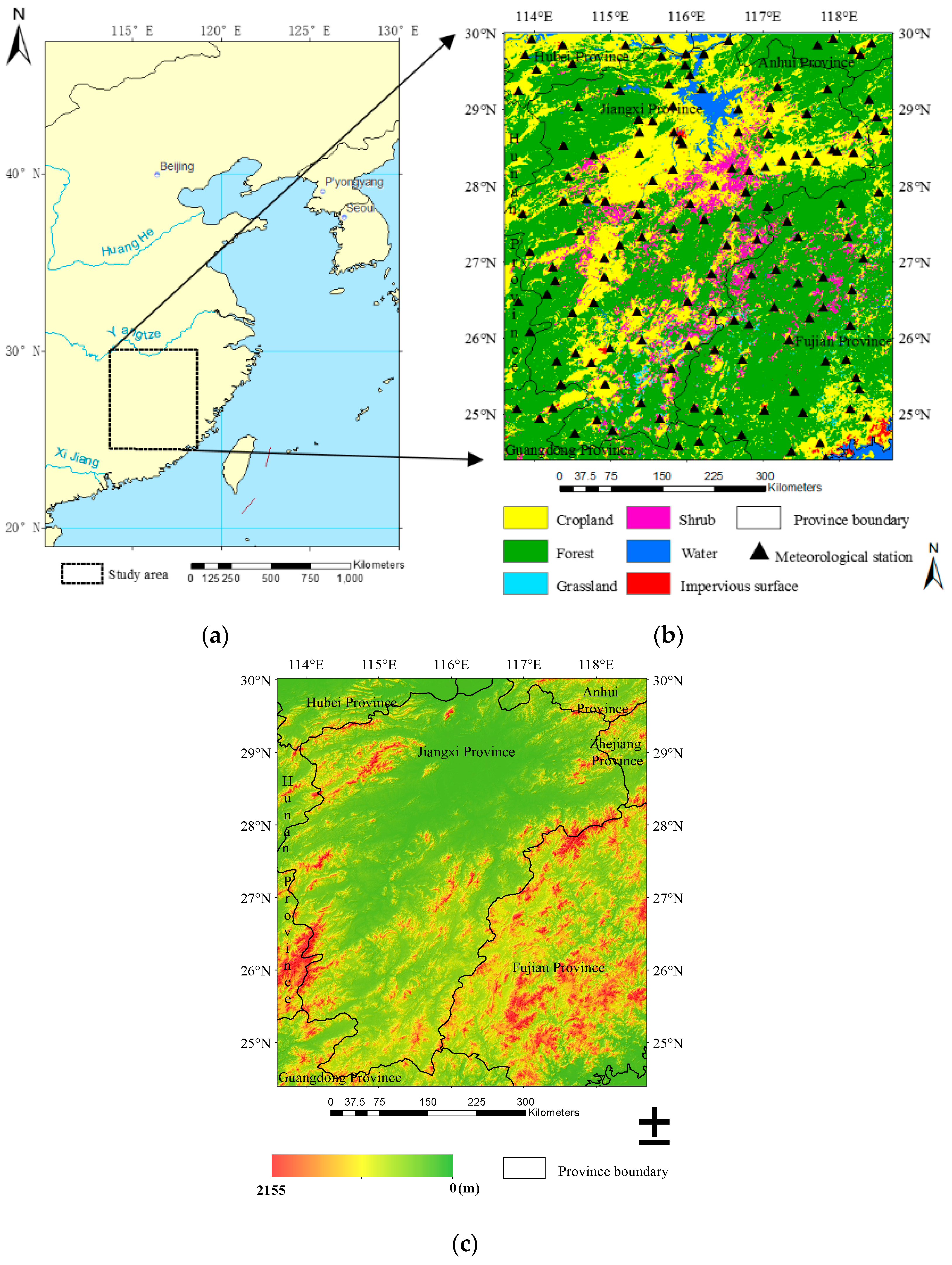
2.1. Study Area
2.2. Air Temperature Meteorological Station Data
2.3. MODIS Land Surface Temperature (LST) Data
2.4. Land-Cover Map
2.5. Model Development and Validation
3. Results
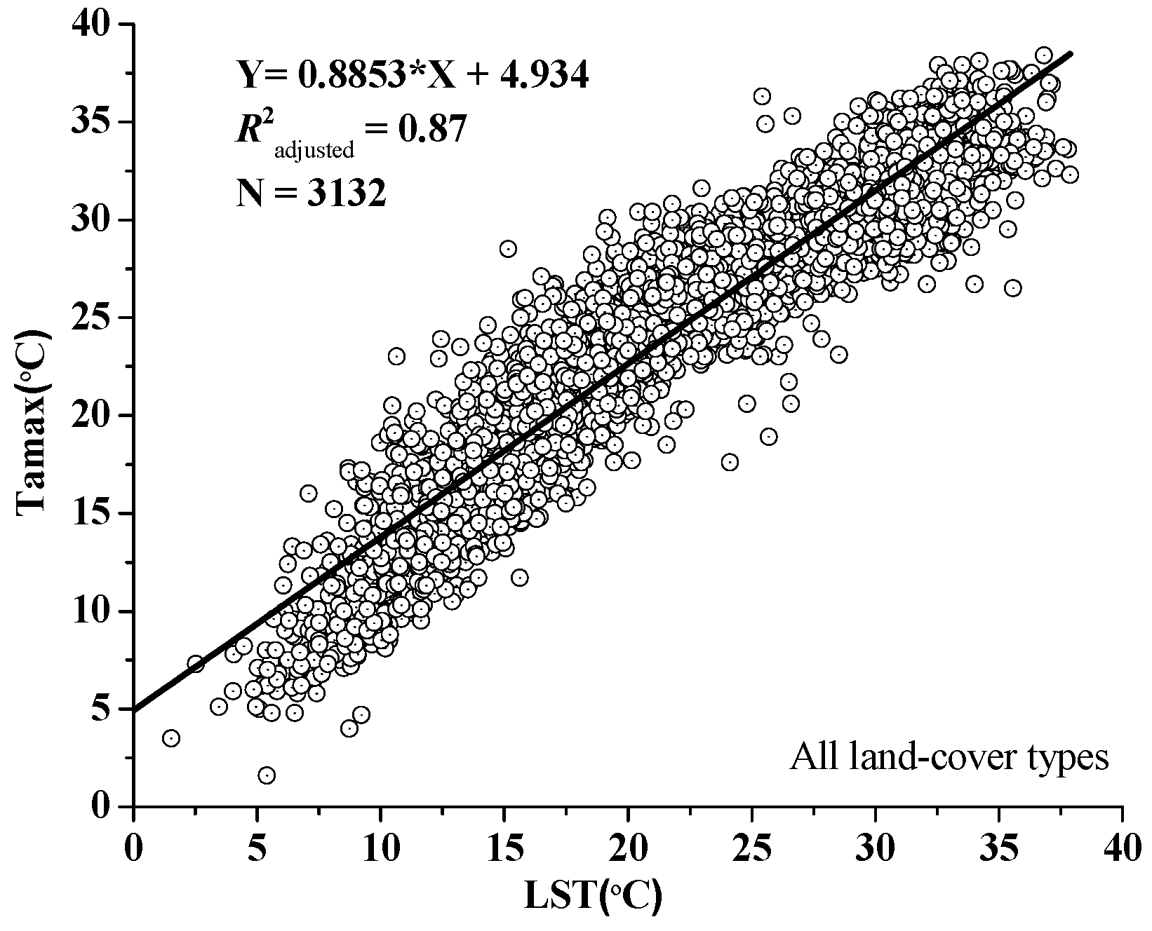
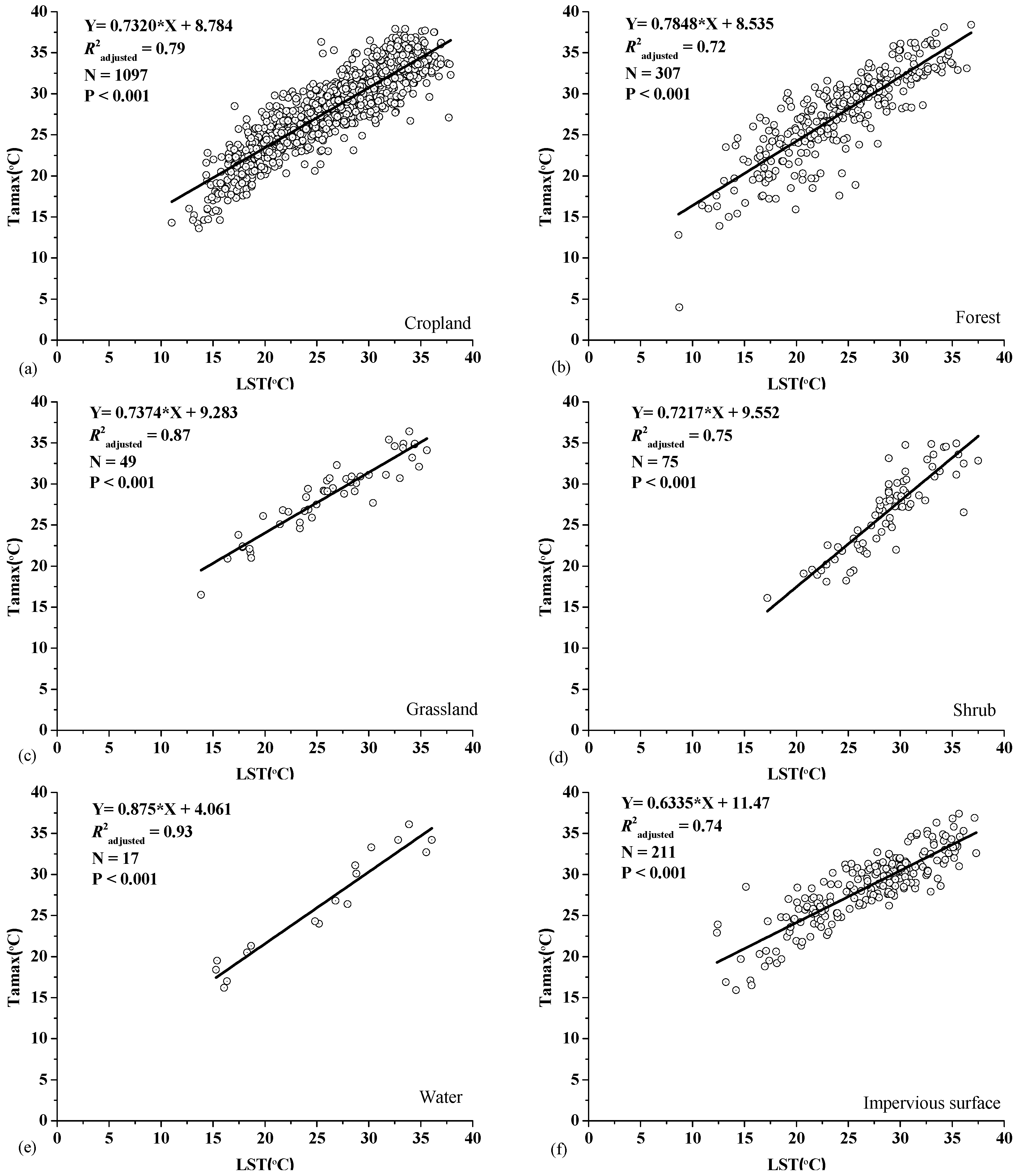
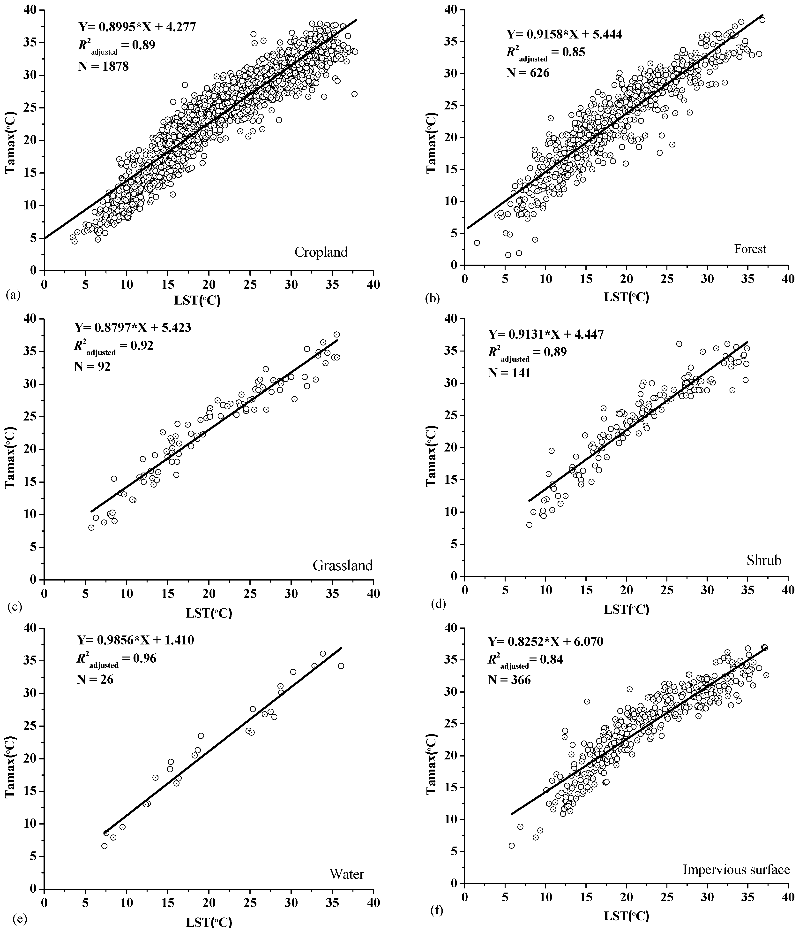
3.1. Estimation of Maximum Air Temperature for Major Land-Cover Types
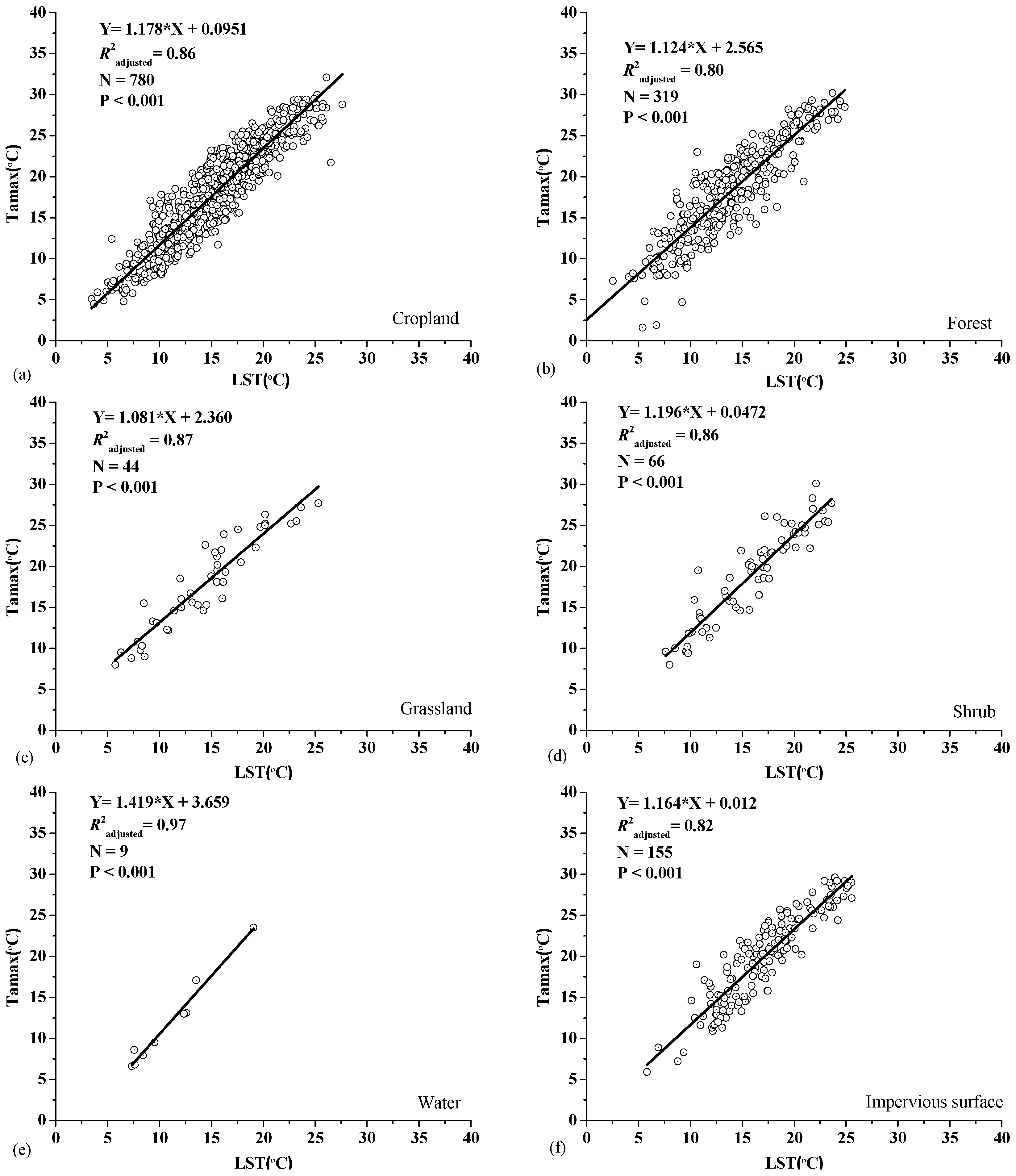
3.2. Estimation of Maximum Air Temperature for Growing and Non-Growing Seasons
4. Discussion
4.1. Impact of Land Cover on the Estimation of Maximum Air Temperature
4.2. Impact of Seasonal Variation on the Estimation of Maximum Air Temperature
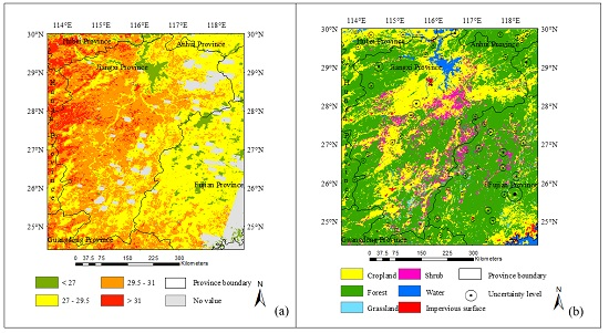
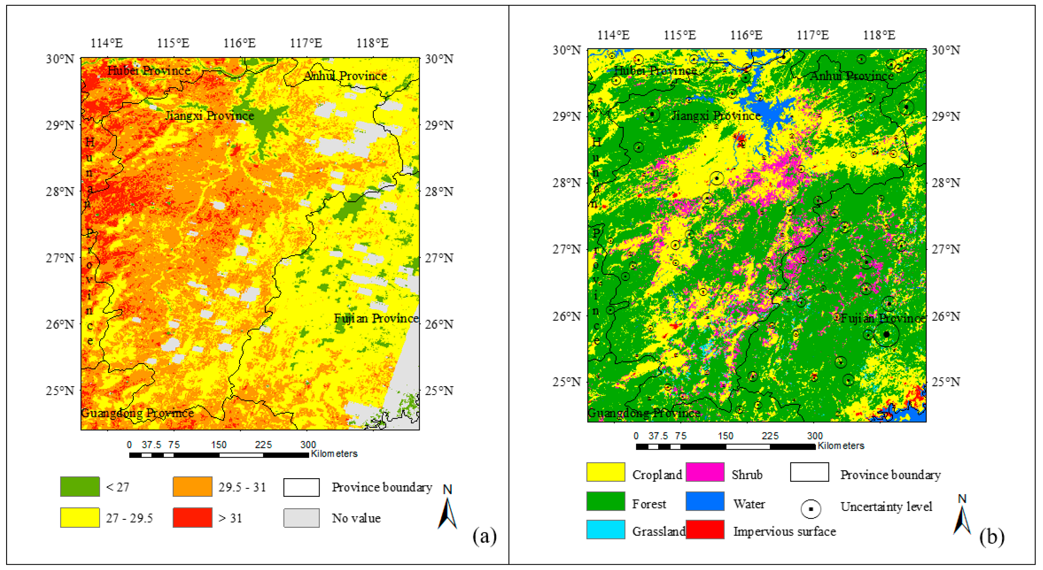
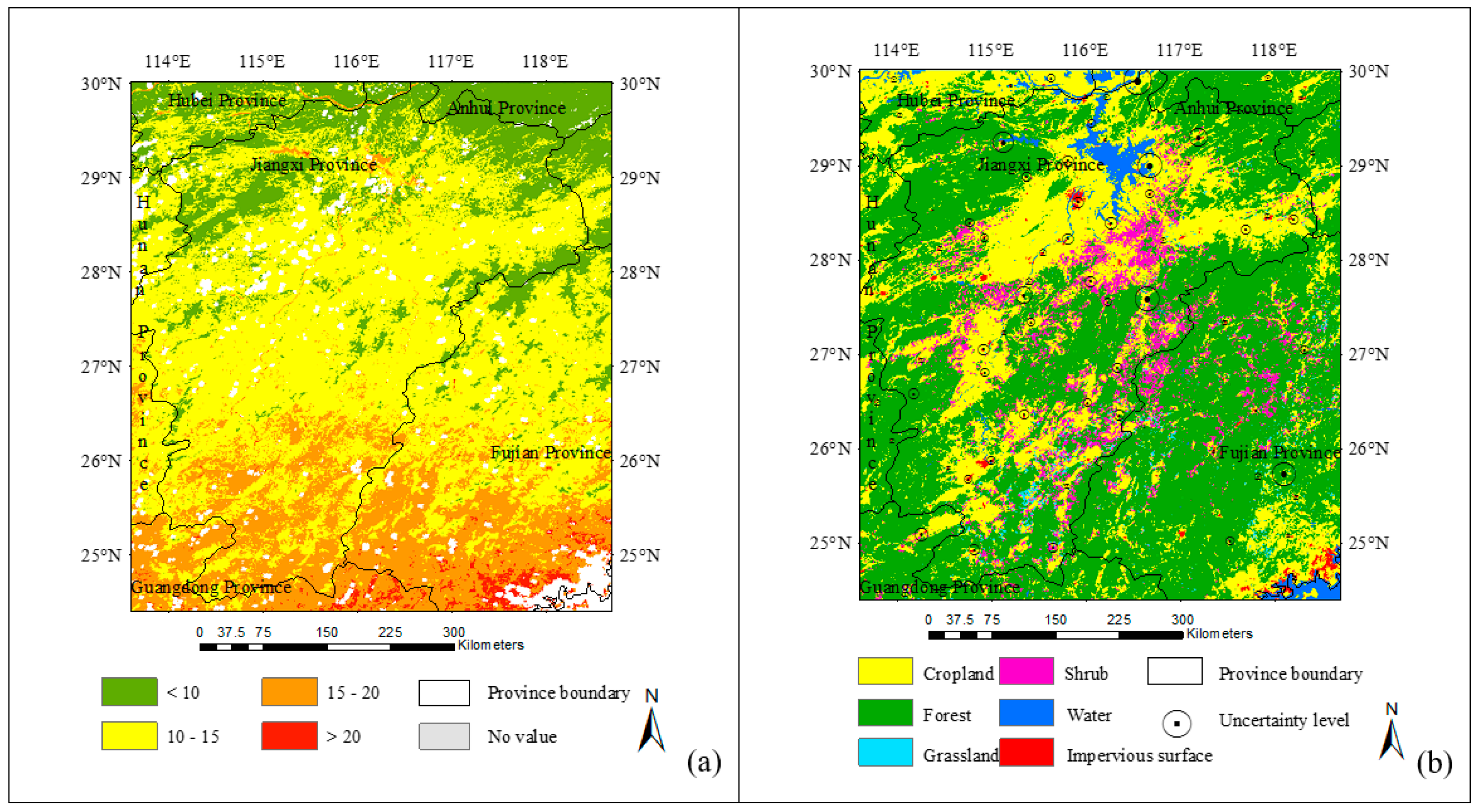
4.3. Spatial Uncertainties in the Estimation of Maximum Air Temperature
5. Conclusions
Acknowledgments
Author Contributions
Conflicts of Interest
References
- Core Writing Team; Pachauri, R.K.; Meyer, L.A. Climate Change 2014. Synthesis Report. Contribution of Working Groups I, II and III to the Fifth Assessment Report of the Intergovernmental Panel on Climate Change; Intergovernmental Panel on Climate Change (IPCC): Geneva, Switzerland, 2014. [Google Scholar]
- Dai, A. Increasing drought under global warming in observations and models. Nat. Clim. Chang. 2013, 3, 52–58. [Google Scholar] [CrossRef]
- Sheffield, J.; Wood, E.F.; Roderick, M.L. Little change in global drought over the past 60 years. Nature 2012, 491, 435–438. [Google Scholar] [CrossRef] [PubMed]
- Nes, E.H.V.; Scheffer, M.; Brovkin, V.; Lenton, T.M.; Ye, H.; Deyle, E.; Sugihara, G. Causal feedbacks in climate change. Nat. Clim. Chang. 2015, 5, 445–448. [Google Scholar]
- Mo, M.C.; Lettenmaier, D.P. Hydrologic Prediction over the Conterminous United States Using the National Multi-Model Ensemble. J. Hydrometeorol. 2014, 15, 1457–1472. [Google Scholar] [CrossRef]
- Weng, Q. Thermal infrared remote sensing for urban climate and environmental studies: Methods, applications, and trends. ISPRS J. Photogramm. Remote Sens. 2009, 64, 335–344. [Google Scholar] [CrossRef]
- Rajasekar, U.; Weng, Q. Urban heat island monitoring and analysis using a non-parametric model: A case study of Indianapolis. ISPRS J. Photogramm. Remote Sens. 2009, 64, 86–96. [Google Scholar] [CrossRef]
- Pichierri, M.; Bonafoni, S.; Biondi, R. Satellite air temperature estimation for monitoring the canopy layer heat island of Milan. Remote Sens. Environ. 2012, 127, 130–138. [Google Scholar] [CrossRef]
- Keramitsoglou, I.; Kiranoudis, C.T.; Sismanidis, P.; Zakšek, K. An Online System for Nowcasting Satellite Derived Temperatures for Urban Areas. Remote Sens. 2016, 8, 306. [Google Scholar] [CrossRef]
- Goetz, S.J.; Prince, S.D.; Small, J. Advances in satellite remote sensing of environmental variables for epidemiological applications. Adv. Parasitol. 2000, 47, 289–307. [Google Scholar] [PubMed]
- Shamir, E.; Georgakakos, K.P. MODIS Land Surface Temperature as an index of surface air temperature for operational snowpack estimation. Remote Sens. Environ. 2014, 152, 83–98. [Google Scholar] [CrossRef]
- Stahl, K.; Moore, R.D.; Floyer, J.A.; Asplin, M.G.; McKendry, I.G. Comparison of Approaches for Spatial Interpolation of Daily Air Temperature in a Large Region with Complex Topography and Highly Variable Station Density. Agric. For. Meteorol. 2006, 139, 224–236. [Google Scholar] [CrossRef]
- Wan, Z.; Dozier, J. A generalized split-window algorithm for retrieving land-surface temperature from space. IEEE Trans. Geosci. Remote Sens. 1996, 34, 892–905. [Google Scholar]
- Wan, Z.; Li, Z.-L. A physics-based algorithm for retrieving land-surface emissivity and temperature from EOS/MODIS data. IEEE Trans. Geosci. Remote Sens. 1997, 35, 980–996. [Google Scholar]
- Vogt, J.; Viau, A.A.; Paquet, F. Mapping regional air temperature fields using satellite derived surface skin temperatures. Int. J. Climatol. 1997, 17, 1559–1579. [Google Scholar] [CrossRef]
- Mostovoy, G.V.; King, R.L.; Reddy, K.R.; Kakani, V.G.; Filippova, M.G. Statistical estimation of daily maximum and minimum air temperatures from MODIS LST data over the state of Mississippi. GISci. Remote Sens. 2006, 43, 78–110. [Google Scholar] [CrossRef]
- Bechtel, B.; Wiesner, S.; Zakšek, K. Estimation of Dense Time Series of Urban Air Temperatures from Multitemporal Geostationary Satellite Data. IEEE J. Sel. Top. Appl. Earth Obs. Remote Sens. 2014, 7, 4129–4137. [Google Scholar] [CrossRef]
- Fan, N.; Xie, G.; Li, W.; Zhang, Y.; Zhang, C.; Li, N. Mapping Air Temperature in the Lancang River Basin Using the Reconstructed MODIS LST Data. J. Resour. Ecol. 2014, 5, 253–262. [Google Scholar]
- Zeng, L.; Wardlow, B.D.; Tadesse, T.; Shan, J.; Hayes, M.J.; Li, D.; Xiang, D. Estimation of Daily Air Temperature Based on MODIS Land Surface Temperature Products over the Corn Belt in the US. Remote Sens. 2015, 7, 951–970. [Google Scholar] [CrossRef]
- Chen, Y.; Quan, J.; Zhan, W.; Guo, Z. Enhanced Statistical Estimation of Air Temperature Incorporating Nighttime Light Data. Remote Sens. 2016, 8, 656. [Google Scholar] [CrossRef]
- Jang, J.D.; Viau, A.A.; Anctil, F. Neural network estimation of air temperatures from AVHRR data. Int. J. Remote Sens. 2004, 25, 4541–4554. [Google Scholar] [CrossRef]
- Meyer, H.; Katurji, M.; Appelhans, T.; Müller, M.U.; Nauss, T.; Roudier, P.; Zawar-reza, P. Mapping daily air temperature for Antarctica based on MODIS LST. Remote Sens. 2016, 8, 732. [Google Scholar] [CrossRef]
- Zaksek, K.; Schroedter-Homscheidt, M. Parameterization of air temperature in high temporal and spatial resolution from a combination of the SEVIRI and MODIS instruments. ISPRS J. Photogramm. Remote Sens. 2009, 64, 414–421. [Google Scholar] [CrossRef]
- Xu, Y.; Qin, Z.; Shen, Y. Study on the estimation of near-surface air temperature from MODIS data by statistical methods. Int. J. Remote Sens. 2012, 33, 7629–7643. [Google Scholar] [CrossRef]
- Benali, A.; Carvalho, A.; Nunes, J. Estimating air surface temperature in Portugal using MODIS LST data. Remote Sens. Environ. 2012, 124, 108–121. [Google Scholar] [CrossRef]
- Chen, F.; Liu, Y.; Liu, Q.; Qin, F. A statistical method based on remote sensing for the estimation of air temperature in China. Int. J. Climatol. 2014, 35, 2131–2143. [Google Scholar] [CrossRef]
- Ho, H.C.; Knudby, A.; Sirovyak, P.; Xu, Y.; Hodul, M.; Henderson, S.B. Mapping maximum urban air temperature on hot summer days. Remote Sens. Environ. 2014, 154, 38–45. [Google Scholar] [CrossRef]
- Xu, Y.; Knudby, A.; Ho, H.C. Estimating daily maximum air temperature from MODIS in British Columbia, Canada. Int. J. Remote Sens. 2014, 35, 8108–8121. [Google Scholar] [CrossRef]
- Noi, P.; Kappas, M.; Degener, J. Estimating Daily Maximum and Minimum Land Air Surface Temperature Using MODIS Land Surface Temperature Data and Ground Truth Data in Northern Vietnam. Remote Sens. 2016, 8, 1002. [Google Scholar] [CrossRef]
- Janatian, N.; Sadeghi, M.; Sanaeinejad, S.H.; Bakhshian, E.; Farid, A.; Hasheminia, S.M.; Ghazanfari, S. A statistical framework for estimating air temperature using MODIS land surface temperature data. Int. J. Climatol. 2016. [Google Scholar] [CrossRef]
- Goward, S.N.; Waring, R.H.; Dye, D.G.; Yang, J. Ecological remote sensing at OTTER: Satellite macroscale observations. Ecol. Appl. 1994, 4, 322–343. [Google Scholar] [CrossRef]
- Prihodko, L.; Goward, S.N.Z. Estimation of air temperature from remotely sensed surface observations. Remote Sens. Environ. 1997, 60, 335–346. [Google Scholar] [CrossRef]
- Vancutsem, C.; Ceccato, P.; Dinku, T.; Connor, S. Evaluation of MODIS land surface temperature data to estimate air temperature in different ecosystems over Africa. Remote Sens. Environ. 2010, 114, 449–465. [Google Scholar] [CrossRef]
- Zhu, W.; Lű, A.; Jia, S. Estimation of daily maximum and minimum air temperature using MODIS land surface temperature products. Remote Sens. Environ. 2013, 130, 62–73. [Google Scholar] [CrossRef]
- Sun, Y.J.; Wang, J.F.; Zhang, R.H.; Gillies, R.R.; Xue, Y.; Bo, Y.C. Air temperature retrieval from remote sensing data based on thermodynamics. Theor. Appl. Climatol. 2005, 80, 37–48. [Google Scholar] [CrossRef]
- Cresswell, M.P. Estimating surface air temperatures, from Meteosat land surface temperatures, using an empirical solar zenith angle. Int. J. Remote Sens. 1999, 20, 1125–1132. [Google Scholar] [CrossRef]
- Shen, S.; Leptoukh, G.G. Estimation of surface air temperature over central and eastern Eurasia from MODIS land surface temperature. Environ. Res. Lett. 2011, 6, 045206. [Google Scholar] [CrossRef]
- Mildrexler, D.J.; Zhao, M.; Running, S.W. A global comparison between station air temperatures and MODIS land surface temperatures reveals the cooling role of forests. J. Geophys. Res. Biogeosci. 2011, 116, 1–15. [Google Scholar] [CrossRef]
- Zhang, W.; Huang, Y.; Yu, Y.; Sun, W. Empirical models for estimating daily maximum, minimum and mean air temperatures with MODIS land surface temperatures. Int. J. Remote Sens. 2011, 32, 9415–9440. [Google Scholar] [CrossRef]
- Urban, M.; Eberle, J.; Hüttich, C.; Schmullius, C.; Herold, M. Comparison of Satellite-Derived Land Surface Temperature and Air Temperature from Meteorological Stations on the Pan-Arctic Scale. Remote Sens. 2013, 5, 2348–2367. [Google Scholar] [CrossRef]
- Kloog, I.; Nordio, F.; Coull, B.A.; Schwartz, J. Predicting spatiotemporal mean air temperature using MODIS satellite surface temperature measurements across the Northeastern USA. Remote Sens. Environ. 2014, 150, 132–139. [Google Scholar] [CrossRef]
- Pielke, R.A.; Davey, C.A.; Niyogi, D.; Fall, S.; Steinweg-Woods, J.; Hubbard, K.; Lin, X.; Cai, X.; Lim, Y.; Li, H.; et al. Unresolved issues with the assessment of multidecadal global land surface temperature trends. J. Geophys. Res. Almos. 2017, 112, 177–180. [Google Scholar] [CrossRef]
- Wei, W.; Chang, Y.; Dai, Z. Streamflow changes of the Changjiang (Yangtze) River in the recent 60 years: Impacts of the East Asian summer monsoon, ENSO, and human activities. Q. Int. 2014, 336, 98–107. [Google Scholar] [CrossRef]
- Gu, C.; Hu, L.; Zhang, X.; Wang, X.; Guo, J. Climate change and urbanization in the Changjiang River Delta. Habitat Int. 2011, 35, 544–552. [Google Scholar] [CrossRef]
- Guo, H.; Hu, Q.; Jiang, T. Annual and seasonal streamflow responses to climate and land-cover changes in the Poyang Lake basin, China. J. Hydrol. 2008, 355, 106–122. [Google Scholar] [CrossRef]
- Shankman, D.; Keim, B.D.; Song, J. Flood frequency in China’s Poyang Lake region: Trends and teleconnections. Int. J. Climatol. 2006, 26, 1255–1266. [Google Scholar] [CrossRef]
- Sun, S.; Chen, H.; Ju, W.; Yu, M.; Hua, W.; Yin, Y. On the attribution of the changing hydrological cycle in Poyang Lake Basin, China. J. Hydrol. 2014, 514, 214–225. [Google Scholar] [CrossRef]
- Fu, G.; Shen, Z.; Zhang, X.; Shi, P.; Zhang, Y.; Wu, J. Estimating air temperature of an alpine meadow on the Northern Tibetan Plateau using MODIS land surface temperature. Acta Ecol. Sin. 2011, 3, 8–13. [Google Scholar] [CrossRef]
- Wan, Z. New refinements and validation of the MODIS Land-Surface Temperature/Emissivity products. Remote Sens. Environ. 2008, 112, 59–74. [Google Scholar] [CrossRef]
- Coll, C.; Caselles, V.; Galve, J.M.; Valor, E.; Niclos, R.; Sanchez, J.M.; Rivas, R. Ground measurements for the validation of land surface temperatures derived from AATSR and MODIS data. Remote Sens. Environ. 2005, 97, 288–300. [Google Scholar] [CrossRef]
- Gong, P.; Wang, J.; Yu, L.; Zhao, Y.C.; Zhao, Y.Y.; Liang, L.; Niu, Z.G.; Huang, X.M.; Fu, H.H.; Liu, S.; et al. Finer resolution observation and monitoring of global land cover: First mapping results with Landsat TM and ETM+ data. Int. J. Remote Sens. 2013, 34, 2607–2654. [Google Scholar] [CrossRef]
- Yu, L.; Liang, L.; Wang, J.; Zhao, Y.Y.; Cheng, Q.; Hu, L.Y.; Liu, S.; Yu, L.; Wang, X.Y.; Zhu, P.; et al. Meta-discoveries from a synthesis of satellite-based land cover mapping research. Int. J. Remote Sens. 2014, 35, 4573–4588. [Google Scholar] [CrossRef]
- Lu, P.; Xie, C. The current situation and quality improving strategy of forest resources in Jiangxi Province. J. Fujian Forest. Sci. Technol. 2008, 35, 259–262. [Google Scholar]
- Wei, W.; Wang, P.; Guo, H. Forest Carbon Sink of Jiangxi Province Based on Forest Resource Inventory Data. Meteorol. Dis. Reduct. Res. 2008, 31, 18–23. [Google Scholar]
- Wu, D.; Shao, Q.Q.; Li, J.; Liu, J.Y. Carbon fixation estimation for the main plantation forest species in the red soil hilly region of southern-central Jiangxi Province, China. Acta Ecol. Sin. 2012, 32, 142–150. [Google Scholar]
- Huang, Z.Q.; Lu, L.; Dai, N.H.; Jiao, G.Y. Vacancy analysis on the development of nature reserves in Jiangxi Province. Acta Ecol. Sin. 2014, 34, 3099–3106. [Google Scholar]
- Guo, Y.; Yan, Y.; Lei, P.; Yuan, R.; Wu, S. The forest stock volume composition characteristics along altitudinal gradient on the northwest slope of Huanggang Mountain in Wuyi mountain of Jiangxi province. South China Forest. Sci. 2015, 5, 10–17. [Google Scholar]
- Jiangxi Provincial Bureau of Statistics. Jiangxi Statistical Yearbook. 2015. Available online: http://www.jxstj.gov.cn/resource/nj/2015CD/indexch.htm (accessed on 8 July 2016). [Google Scholar]
- Fujian Provincial Bureau of Statistics. Fujian Statistical Yearbook. 2015. Available online: http://www.stats-fj.gov.cn/tongjinianjian/dz2015/index-cn.htm (accessed on 8 July 2016). [Google Scholar]
- Godwin, C.; Chen, G.; Singh, K.K. The impact of urban residential development patterns on forest carbon density: An integration of LiDAR, aerial photography and field mensuration. Landsc. Urban Plan. 2015, 136, 97–109. [Google Scholar] [CrossRef]
- Johnson, K.R.; Ingram, B.L. Spatial and temporal variability in the stable isotope systematics of modern precipitation in China: implications for paleoclimate reconstructions. Earth Planet. Sci. Lett. 2004, 220, 365–377. [Google Scholar] [CrossRef]
- Liu, Q.; Yang, Z.; Cui, B. Spatial and temporal variability of annual precipitation during 1961–2006 in Yellow River Basin, China. J. Hydrol. 2008, 361, 330–338. [Google Scholar] [CrossRef]
- Lee, X.; Goulden, M.L.; Hollinger, D.Y.; Barr, A.; Black, T.A.; Bohrer, G.; Bracho, R.; Drake, B.; Goldstein, A.; Gu, L.; et al. Observed increase in local cooling effect of deforestation at higher latitudes. Nature 2011, 497, 384–387. [Google Scholar] [CrossRef] [PubMed]


| Land-Cover Type | Cropland | Forest | Grassland | Shrub | Water | Impervious Surface |
|---|---|---|---|---|---|---|
| Percentage (%) | 29.27 | 60.81 | 1.21 | 5.78 | 2.29 | 0.63 |
| Area (km2) | 92,158 | 191,459 | 3817 | 18,191 | 7215 | 1985 |
| Land-Cover Type | R2adjusted | MAE (°C) | RMSE (°C) | Change in MAE (%) | Change in RMSE (%) |
|---|---|---|---|---|---|
| All combined | 0.87 | 2.04 | 2.55 | \ | \ |
| Cropland | 0.89 | 1.97 | 2.42 | 3.4 | 5.1 |
| Forest | 0.85 | 2.35 | 3.05 | −15.2 | −19.6 |
| Grassland | 0.92 | 1.89 | 2.40 | 7.4 | 5.9 |
| Shrub | 0.89 | 2.01 | 2.45 | 1.5 | 3.9 |
| Water | 0.96 | 1.93 | 2.22 | 5.4 | 12.9 |
| Impervious surface | 0.84 | 1.98 | 2.48 | 2.9 | 2.8 |
© 2017 by the authors. Licensee MDPI, Basel, Switzerland. This article is an open access article distributed under the terms and conditions of the Creative Commons Attribution (CC BY) license ( http://creativecommons.org/licenses/by/4.0/).
Share and Cite
Cai, Y.; Chen, G.; Wang, Y.; Yang, L. Impacts of Land Cover and Seasonal Variation on Maximum Air Temperature Estimation Using MODIS Imagery. Remote Sens. 2017, 9, 233. https://doi.org/10.3390/rs9030233
Cai Y, Chen G, Wang Y, Yang L. Impacts of Land Cover and Seasonal Variation on Maximum Air Temperature Estimation Using MODIS Imagery. Remote Sensing. 2017; 9(3):233. https://doi.org/10.3390/rs9030233
Chicago/Turabian StyleCai, Yulin, Gang Chen, Yali Wang, and Li Yang. 2017. "Impacts of Land Cover and Seasonal Variation on Maximum Air Temperature Estimation Using MODIS Imagery" Remote Sensing 9, no. 3: 233. https://doi.org/10.3390/rs9030233
APA StyleCai, Y., Chen, G., Wang, Y., & Yang, L. (2017). Impacts of Land Cover and Seasonal Variation on Maximum Air Temperature Estimation Using MODIS Imagery. Remote Sensing, 9(3), 233. https://doi.org/10.3390/rs9030233