Bohai Sea Ice Parameter Estimation Based on Thermodynamic Ice Model and Earth Observation Data

Abstract

We estimate two essential sea ice parameters—namely, sea ice concentration (SIC) and sea ice thickness (SIT)—for the Bohai Sea using a combination of a thermodynamic sea ice model and Earth observation (EO) data from synthetic aperture radar (SAR) and microwave radiometer. We compare the SIC and SIT estimation results with in-situ measurements conducted in the study area and estimates based on independent EO data from near-infrared/optical instruments. These comparisons suggest that the SAR-based discrimination between sea ice and open-water works well, and areas of thinner and thicker ice can be distinguished. A larger comprehensive training dataset is needed to set up an operational algorithm for the estimation of SIC and SIT.

1. Introduction

A large portion of the Bohai Sea is typically covered by sea ice during the winter from December to March. The average level-ice thickness can be as thick as 20 to 40 cm depending on the weather conditions [1], and the maximum thickness can reach 50 cm in very cold winters [2]. The maximum ice extent often occurs in early February. A large portion of the Bohai Sea is covered by sea ice during normal winters. This sea ice causes serious hazards for marine transportation, offshore oil/gas production, the fishing industry, and coastal construction [3]. Even in mild winters, sea ice can damage certain off-shore activities. Therefore, operational monitoring of sea ice conditions is of high importance, and has been carried out for many years [4,5]. In-situ sea ice observations are conducted in the coastal regions, and ice thickness and drift measurements are also carried out at off-shore oil platforms. Satellite remote sensing data from optical/near-infrared sensors such as the Moderate Resolution Imaging Spectroradiometer (MODIS) and microwave sensors (radiometers, radars) have been utilized for retrieving various sea ice parameters, such as sea ice type, ice concentration, as well as ice thickness and extent.

In this paper, we present new empirical methods to retrieve sea ice concentration (SIC) and sea ice thickness (SIT) in the Bohai Sea using synthetic aperture radar (SAR) imagery, microwave radiometer data, and a thermodynamic sea ice model. We targeted the winter of 2012–2013 due to the availability of RADARSAT-2 (RS-2) ScanSAR imagery over the Bohai Sea. The resulting SIC and SIT maps are compared to those estimated from fine-resolution MODIS and HuanJing-1B imagery, and to in-situ measurements.

We thus first present an overview of previous studies on SIC and SIT estimation using Earth Observation (EO) data and focusing mainly on the Bohai Sea ice. Section 2 describes our study area, and in Section 3 the data sets and their pre-processing methods. Our novel methods for SIC and SIT retrieval, examples of the SIC and SIT charts, and their validation studies are presented in Section 4. An estimation of the Bohai Sea ice volume based on the SIC and SIT retrievals is presented in Section 5. In Section 6 (Discussion), we compare our methods and results to previous work, and finally, we give our conclusions in Section 7.

1.1. Overview of Previous Studies on Sea Ice Concentration and Thickness Retrieval

1.1.1. Sea Ice Concentration

The current operational SIC products are based on microwave radiometer data with a spatial resolution on the order of 6.25 to 25 km (e.g., [6,7]). SIC in a finer resolution can be retrieved from optical or thermal infrared imagery [8], but its acquisition requires cloud-free conditions, and in addition, optical imaging is possible only in daylight conditions. These circumstances typically lead to long temporal data gaps over an area of interest. So far, SAR imagery with fine spatial resolution, large spatial coverage, and the capability to acquire data through cloud cover, has not been widely used for the SIC estimation. Some studies on using single-band SAR for the SIC estimation have, however, been conducted [9,10,11,12,13,14,15,16,17]. Automated sea ice classification schemes—which implicitly include SIC or an open-water class—based on single-band SAR texture have been proposed [18,19,20,21,22,23,24]. These methods use multiple techniques such as the gray-level co-occurrence texture features [25], Markov random fields [26], and Gabor filters [18,27] to classify the SAR imagery. It has been shown that open-water detection and SIC estimates that are based solely on SAR co-polarized (HH) channel backscattering magnitude can be improved by including cross-polarized (HV) channel information. Especially at incidence angles lower than 35 degrees, the HV imagery contains complementary sea ice information [28]. In low-to-moderate wind conditions, backscattering from open-water is typically strong at co-polarized channels (HH or VV), but low at cross-polarized channels, thereby allowing improvement in open water detection [29,30]. Better SIC estimation results can be achieved by using a combination of HH and HV (or VV and VH) channels, radar incidence angle information, and texture features (contextual information), such as auto-correlation (AC) [10,11,31]. Additionally, the co-polarization ratio (VV/HH) can be used to improve open-water detection and sea ice classification based on the SAR backscattering magnitude alone [32]. A recently case study proposed the utilization of deep convolutional neural networks for the estimation of SIC [33].

We thus conclude that the SIC estimation using RS-2 C-band dual-polarization (HH, HV) SAR imagery should be based—in addition to backscattering levels—on multiple segment-wise textural features. For the development of an empirical SIC estimation method, high-quality reference data (based on in-situ observations or reliable EO data) are indeed needed.

1.1.2. Sea Ice Thickness

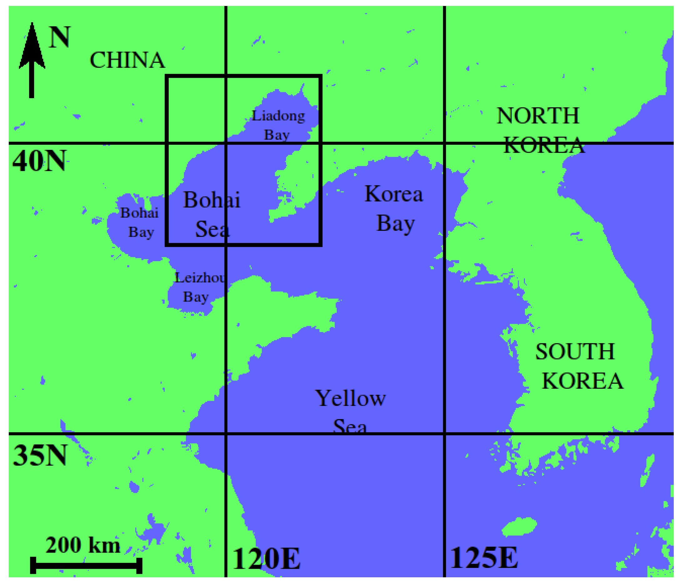
Space-borne remote sensing of SIT can be conducted based on Archimedes’ law and satellite radar or laser altimeter measurements of sea ice freeboard [34,35,36]. However, this method produces large relative errors for thin-ice [34], and is thus not suitable for the Bohai Sea where only thin first year ice occurs. A recent study [37] concluded that high-frequency (36 and 89 GHz) microwave radiometer data can be used to identify thin-ice (<30 cm) areas within thicker ice fields with reasonable accuracy; however, the thickness of the thin-ice can not be estimated. Low frequency L-band radiometer data from Soil Moisture and Ocean Salinity (SMOS) satellite have been used to retrieve ice thickness up to half a meter [38], but the spatial resolution of the SMOS data (30–50 km) is too coarse for the Bohai Sea. Estimation of thin-ice thickness can be also conducted using satellite infrared imagery-based ice surface temperatures ($T_s$), together with atmospheric forcing data through an ice surface heat balance equation [39,40]. This method is suitable for monitoring level-ice SIT in the Bohai Sea under cold weather conditions [41]. SIT can also be estimated using optical spectrometer data through the empirical relationships between sea ice reflectance spectra or albedo and SIT [42,43,44,45]. However, the resulting SIT estimates may have large errors due to impurities (sand, dissolved organic matter) in the Bohai Sea ice, which then reduce the surface albedo [46]. In addition, the effect of a possible snow layer on thin sea ice is currently omitted in these empirical models.

Estimation of SIT using SAR data (from single polarization data to multi-frequency polarimetric data) has been investigated in many case studies, but no operational methods solely based on SAR data exist to date. It has been demonstrated that estimation of deformed ice thickness for the Baltic Sea under dry snow conditions is possible through a statistical relationship between SAR backscatter and mean freeboard (proportional to SIT) [47]. Another simple SIT estimation method is based on the relationship between the co-polarization ratio and level-ice SIT [48]. The co-polarization ratio is correlated with the SIT through its physical relationship with sea ice surface salinity, which determines the ice surface dielectric constant.

A sea ice backscattering model has been combined with a sea ice thermodynamic model to assess the determination of thin-ice thickness in the Bohai Sea based on SAR data at different frequencies, polarizations, and incidence angles [49]. These results suggest that the co-polarization ratio can be used to retrieve thin-ice thickness from C- and X-band SAR, while the co-polarization correlation coefficient can be used to retrieve thin-ice thickness from L-, C-, and X-band SAR. Zhang et al. [50] presented a three-component scattering model to decompose the RS-2 polarimetric SAR data of sea ice into an incoherent summation of surface, double-bounce, volume, and residual scattering components. The proposed polarimetric decomposition approach helped distinguish different ice types and offered a proxy for SIT (>10 cm) estimation.

SIT estimation using SAR imagery and SIT background data from ice charts or sea ice models, or using SAR along with other sensor data have also been studied. For the Baltic Sea, an operational level-ice thickness chart is provided daily. It combines the SIT information from the Finnish Ice Service (FIS) ice chart (mainly manual interpretation) and C-band SAR imagery [51,52]. The SAR images are used to spatially produce a more accurate level-ice thickness chart (around 500 m resolution) than that given by the FIS ice chart (resolution ≈10 km). Karvonen et al. [14] studied ice thickness estimation in the Gulf of St. Lawrence using HH-polarized RS-2 imagery together with a background level ice SIT field based on a thermodynamic sea ice model.

In summary, SIT estimation for the Bohai Sea from SAR data seems to be feasible even with a simple empirical relationship between SIT and SAR data. However, the development of such a relationship requires an extensive in-situ data set on SIT or ice surface topography. The co-polarization ratio (HH/VV) has shown promise for direct SIT estimation, but simultaneous HH- and VV-polarization SAR data are unfortunately not currently operationally available.

We therefore suggest that the most promising approach for an operational SIT estimation over the Bohai Sea is based on dual-polarization (HH and HV) imagery available from RS-2 (used here) or SENTINEL-1 SAR and a SIT background field derived from an ice chart (as has been conducted for the Baltic Sea [53,54]), or from a sea ice model, as for the Barents and Kara Seas [55,56]. SAR backscatter statistics are used to modify this background SIT field into a finer spatial resolution.

2. Study Area

Our study area here is Liaodong Bay in the Bohai Sea, which is at least partly ice covered every winter season (Figure 1). The entire Liaodong Bay has been covered in the past by sea ice during severe winters (e.g., 1936, 1947, and 1969). According to oil platform weather station data during our study period of January–February 2013, daily mean air temperatures were around −10 ${}^{°}$C in January and around −5 ${}^{°}$C during the first 10 days of February, then increased to 0 ${}^{°}$C and even higher by mid-February.

In general, the ice season of 2012–2013 was severe in Liaodong Bay. Sea ice appeared on 4 December 2012 and disappeared on 20 March 2013; i.e., the whole ice season lasted 106 days. On 8 February 2013, the sea ice extent reached the annual maximum and started to retreat about a week later. The ice conditions over the west coast were more severe than the climatological average, while ice conditions over the east coast were milder than those close to the west coast.

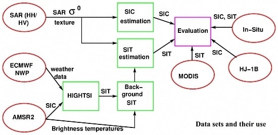
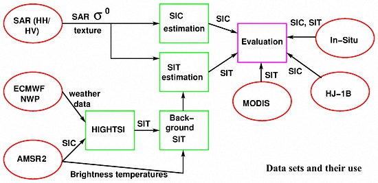
3. Data Sets and Their Processing

In this section, we describe the data sets used in the SIC and SIT estimation and validation over the Bohai Sea. RADARSAT-2 SAR imagery was the basis for both SIC and SIT retrieval. AMSR2 radiometer data and the thermodynamic ice model HIGHTSI (High-Resolution Thermodynamic Snow/Ice model) were used to construct a background ice thickness field for the SAR-based SIT retrieval. In-situ data and SIC and SIT estimates from the MODIS and Chinese HuanJing-1B (HJ-1B) optical imagery were utilized in the evaluation (including both visual assessment and numerical validation) of the SIC and SIT retrieval methods. The HIGHTSI model used the European Centre for Medium-Range Weather Forecasts (ECMWF) ERA-Interim reanalysis data and a SIC product based on the AMSR2 radiometer [7] as its input. A general diagram of the SIC and SIT estimation algorithms with the used datasets is presented in Figure 2.

3.1. RADARSAT-2 SAR

RADARSAT-2 (RS-2) has a dual-polarized mode in ScanSAR Wide (SCW) mode imaging, enabling acquisition of HH/HV (transmitting horizontal polarization, H, and receiving both horizontal H- and vertical V-polarization) or VV/VH (transmitting V polarization, and receiving both V- and horizontal H-polarization) polarization combinations with a wide swath width of approximately 500 km. This RS-2 mode with a large spatial cover is especially suitable for operational sea ice monitoring. We used eleven RADARSAT-2 ScanSAR Wide mode images with HH/HV combination, acquired during the period from 2 January to 19 February 2013. The SAR images, their acquisition times, orbit (ascending/descending), and center locations are listed in

Table 1. RADARSAT-2 ScanSAR Wide mode SAR imagery acquired over the Bohai Sea in January–February 2013. All the SAR imagery were acquired with HH/HV polarization combination (dual-polarized data).

Date	Acquisition Start Time (UTC)	Orbit	Center (Lat, Long) (${}^{\circ }$)
2 January 2013	09:56:20	Ascending	38.85 N, 120.05 E
6 January 2013	21:53:00	Descending	38.89N, 122.89E
9 January 2013	22:06:16	Descending	39.18N, 119.79E
16 January 2013	22:02:01	Descending	39.29N, 120.87E
23 January 2013	21:57:52	Descending	39.16N, 121.88E
26 January 2013	09:56:29	Ascending	39.44N, 119.91E
2 February 2013	22:06:14	Descending	39.27N, 119.81E
9 February 2013	22:02:01	Descending	39.30N, 120.86E
12 February 2013	10:00:38	Ascending	39.27N, 118.90E
16 February 2013	21:57:51	Descending	39.14N, 121.88E
19 February 2013	09:56:17	Ascending	38.76N, 120.08E

. SCW mode imagery has a nominal swath width of about 500 km and a pixel spacing of about 50 m. The resolution of these images is 73–163 m (range) by 100 m (azimuth), depending on the incidence angle. The number of equivalent looks was larger than six, and the radiometric error was less than 1 dB [57]. The RADARSAT-2 orbit is sun-synchronous, and the morning passes are in a descending orbit, while evening/afternoon passes have an ascending orbit.

3.1.1. SAR Data Pre-Processing

The SAR data were calibrated and rectified to a latitude–longitude coordinate system. The resolution of the rectified imagery was 100 m (exactly at latitude 39 ${}^{°}$N). After calibration, an incidence angle correction procedure was performed as described in [17]. The correction was linear for the HH channel and nonlinear for the HV channel. The HV channel correction also tried to equalize the HV noise floor.

For the SIC and SIT estimation, the SAR imagery was re-sampled to a reduced resolution of 500 m. The re-sampled SAR images were segmented using the Iterated Conditional Modes (ICM) [58] algorithm. Any small SAR segments with a size less than 100 pixels (corresponding to an area of 25 km${}^2$) were combined to adjacent larger segments with the closest HH-polarization backscattering coefficient via an iterative process. Segmentation was applied to principal component images which combine the HH and HV channel images as a linear combination. The minimum segment size is also 100 pixels, corresponding to an area of 5 × 5 km square.

3.1.2. SAR Features

In addition to the calibrated backscattering coefficients with incidence angle correction, multiple texture features were extracted from the SAR data: entropy, auto-correlation, cross-correlation, and the number of corner points for each segment and variograms. These texture features have been used in the SIC and SIT estimation in our earlier studies (e.g., in [17]). The features are straightforward to compute; the only parameter for them is the size of the feature computation window. We included many features, because in the training phase we used feature selection that was based on varying the number of the features and the selected features. This process guarantees that the best sets of features for the SIC and SIT estimation were selected from all the features involved. The backscattering coefficients are denoted by ${\sigma }_{HH}^0$ and ${\sigma }_{HV}^0$ for the HH and HV polarization channels, respectively. Texture features (auto-correlations and entropies) were computed for full-resolution (100 m) SAR images in regularly-shaped circular windows and then down-sampled to a 500 m resolution. The features were computed in a window with a diameter of 11 pixels (i.e., the window has a radius of 5 pixels and has an odd size such that it has a center point in the middle of a pixel location). The window radius is also equivalent to the down-sampling rate, and adjacent feature windows overlap each other by the radius size in both coordinate directions. This method has proven to be a suitable combination of down-sampling and the window size. The boundaries between fields with different characteristics described by the texture feature are correctly located in the reduced resolution and sharpness. Additionally, the window size is large enough for computing the texture features; smaller window sizes are more sensitive to the radar speckle, while on the other hand larger window sizes lead to coarser resolution with less detail. The window size was also selected based on the properties of the SAR data (needs to be large enough to deal with the speckle and on the other hand be able to locate sea ice details in a high-enough resolution (e.g., for ship navigation in ice). This window size has also been used in the SIC estimation [16,17].

Entropy E was computed as

$$E=-\sum _{k=0}^{255}{p}_{k}lo{g}^2{p}_k,$$

(1)

where $p_k$’s are the proportions of each gray tone k within each computation window [59]. Auto-correlation $C_A$ was computed as

$$C_A(k,l)=\frac{{\sum }_{ij\in W}\left(I(i-k,j-l)-{\mu }_W\right)\left(I(i,j)-{\mu }_W\right)}{|W|{\sigma }_W^2},$$

(2)

where $I(i,j)$ is the pixel value at location $(i,j)$. i and j refer to the row and column coordinates of the image pixel, respectively. k and l here refer to the displacement of the row and column coordinates from $(i,j)$. Mean over the directions horizontal, vertical, and diagonal directions (i.e., $(k,l)=(0,1)$, $(k,l)=(1,0)$, $(k,l)=(1,1)$ and $(k,l)=(1,-1)$) were used because the statistic $C_A$ describes two-dimensional data [31,60]. The size of the computation window W in pixels was denoted by $|W|$. The diameter of the sliding texture feature computation window W was eleven pixels. ${\sigma }_W$ and ${\mu }_W$ are the window mean and standard deviation, respectively.

The cross-correlation $C_c$ between the SAR HH and HV channels—denoted by $I_{HH}$ and $I_{HV}$, respectively, is

$$\begin{array}{c}{C}_c(k,l)=\frac{1}{N{\sigma }_{HH}{\sigma }_{HV}}\times \sum _{i,j\in W}\left(I_{HH}(k+i,l+j)-{\mu }_{HH}\right)\left(I_{HV}(k+i,l+j)-{\mu }_{HV}\right),\end{array}$$

(3)

where N is the number of pixels within the computation window W. Round-shaped windows with a radius of five pixels ($R=5$) were used for $C_c$, and final values of the segment-wise features are the median values of each feature within a segment. The mean values ${\mu }_{HH}$ and ${\mu }_{HV}$ are computed as averages of the pixel values in W. The corner point counts ($N_c$) were also extracted for each segment using local binary patterns [61] in a similar way to what was presented in [62].

The number of corner points with respect to each segment area was computed for both polarization channels and used as texture features. These are denoted by $N_C^{HH}$ and $N_C^{HV}$.

Based on the segmentation result using the ICM method and the above features, the segment-wise median values of each feature were calculated and linearly scaled to 8 bits-per-pixel (bpp) images. $C_A$ and $C_c$ were scaled such that the pixel value of one corresponds to auto-correlation zero and pixel value 255 to 1. The HH (HV) channel entropy was scaled such that pixel value one corresponds to entropy 3.6 (3.2) or less and 255 corresponds to entropy values 5.3 (4.4) or higher. The corner segment-wise counts value 1 corresponds to no corner points and value 255 corresponds to that of all the segment points that are corner points. These scalings were selected experimentally earlier for the Baltic Sea SAR imagery in [17].

We also computed certain features based on variograms which also described the spatial auto-correlation in a slightly different manner. The variograms were locally estimated in a window with a radius of 11 pixels using the original SAR resolution (100 m); the results were down-sampled to 500 m resolution. Assuming a stationary and isotropic process, the variogram γ is (locally) dependent only on the inter-distance (h), and can be estimated as [63]

$$\gamma (h)=\frac{1}{2|N_h|}\sum _{i,j\in N_h}{|z_i-z_j|}^2,$$

(4)

where $z_i$ and $z_j$ are the pixel values at locations i and j, whose distance is h. $N_h$ is the set of pairs of observation z with indices k and l such that $|z_k-z_l|=h$ and $|N_h|$ is the number of such pairs. We modeled the range of the variogram from the origin (nugget) to the sill by fitting a linear variogram as a function of h on this interval. The slope and intercept value of the linear fit were used as features. The slopes and intercepts are referred to here as $V_1^{ch}$ and $V_2^{ch}$, respectively, where the superscript $ch$ is the SAR channel, either HH or HV.

3.2. AMSR2 Radiometer

The AMSR2 level L1B brightness temperature swath data were acquired from JAXA for our study period. The footprints for the AMSR2 L1B data are 7 km by 12 km for the 36 GHz channel and 3 km by 5 km for the 89 GHz channel A- and B-horn data [64]. The 89 GHz channel data were first resampled into a spatial resolution of 3 km and the 36 GHz channel into a spatial resolution of 7 km, and then processed to daily brightness temperature mosaics with an approximately 6 km pixel size for both channels. The AMSR-2 data were used to calculate the polarization ratio (PR) for the 36 GHz channel (i.e., $f=$ 36 Ghz in Equation (5)):

$$\begin{array}{cc}& \mathrm{PR}(f)=\frac{T_{\mathrm{B}}(f,V)-T_{\mathrm{B}}(f,H)}{T_{\mathrm{B}}(f,V)+T_{\mathrm{B}}(f,H)},\hfill \end{array}$$

(5)

and the H-polarized spectral gradient ratio (GR) between 89 and 36 GHZ channels (i.e., $f1=$ 89 GHz, $f2=$ 56 GHz, and $p=$ H in Equation 6):

$$\begin{array}{cc}& \mathrm{GR}(f1,f2,p)=\frac{T_{\mathrm{B}}(f1,p)-T_{\mathrm{B}}(f2,p)}{T_{\mathrm{B}}(f1,p)+T_{\mathrm{B}}(f2,p)}.\hfill \end{array}$$

(6)

The advantage of PRs compared to using brightness temperatures is that it reduces the dependence of the sea ice signatures on snow and ice temperature [65]. The linear discriminant analysis (LDA) score [37] was applied to a combination of PR and GR; for more details, see Section 4.1. The resolution of the LDA score is equivalent to that (6 km) of the PR and GR mosaics. The AMSR2 PR and GR data are used to modify SIT estimates from the HIGHTSI thermodynamic sea ice model. For this, the LDA scores were further interpolated to a 1 km grid.

3.3. HJ-1B Optical Imagery

We used two images from the Chinese HuanJing-1B (HJ-1B) optical sensor for validation of our new SAR-based SIC product. These images were acquired over the Bohai Sea on 9 January 2013 02:09:12 and 02:10:01 (UTC). HJ-1B is equipped with a CCD camera with four bands in the 430–900 nm wavelength range. The spatial resolution of the images is 30 m and the swath width is 360 km.

After radiometric correction, land masking and manual cloud masking, the near-infrared (NIR) band image (band 4) was classified pixel-wise to sea ice and open-water classes with an experimentally defined threshold pixel value of 23. Because the used HJ-1B data was cloud-free and the boundary of sea ice and open-water was very clear, this threshold value could be determined visually. The pixel value describes the surface reflectance, and therefore it is unitless. From the resulting water/sea ice classification, the reference SIC values for each SAR segment were estimated as proportions of the open-water grid points with respect to all the grid points within each SAR segment.

3.4. MODIS Spectrometer Imagery

MODIS spectrometer imagery for cloud-free conditions over the Bohai Sea was processed to pixel-wise open-water-sea ice charts (optical 250 m imagery) and SIT charts (nighttime thermal infrared 1000 m imagery).

3.4.1. MODIS Ice Thickness Charts

We previously developed a SIT retrieval method for the Bohai Sea based on the ice surface temperature from the MODIS thermal infrared imagery [41]. The overall bias and root-mean-squared error of the MODIS SIT charts over the Liaodong Bay was found to be −1.4 cm and 3.9 cm, respectively, compared to in situ observations from two offshore oil platforms during the winter of 2009–2010. Here we processed MODIS SIT charts for the winter of 2013, following the method in [41]. Atmospheric forcing data was from the European Centre for Medium-Range Weather Forecasts (ECMWF) ERA-Interim reanalysis data. We found several good cloud-free MODIS images for estimation of the ice thickness, with four of them matching the dates of the SAR acquisitions. However, SIT estimation based on the MODIS data is not very reliable in such warm air and ice surface temperature conditions [39,40], as was the case during our study period (RS-2 imagery from 2 January to 19 February 2013), and thus only one SIT chart of 9 January 2013 had an accuracy comparable to the charts in [41]. On average, winter in 2009–2010 was significantly colder than the winter of 2013. This one selected MODIS SIT chart is used as reference for visually evaluating the quality of other SIT estimates in our study.

3.4.2. MODIS Optical Imagery Open-Water-Sea Ice Chart

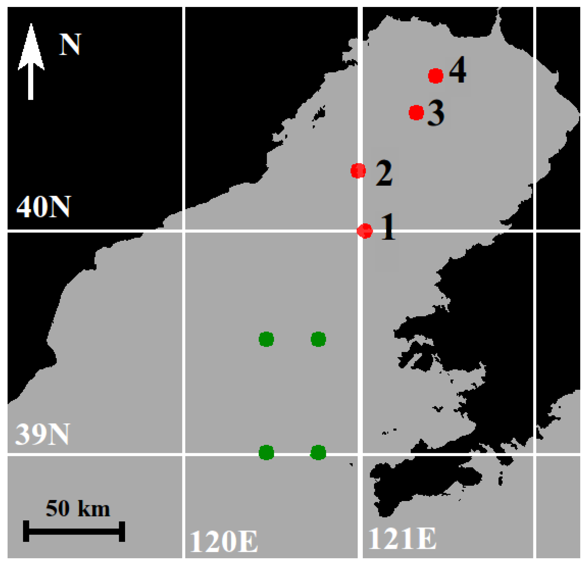
Previously, Su et al. [66] successfully conducted open-water-sea ice classification in the Bohai Sea using MODIS optical imagery from bands 1 (659 nm) and 2 (865 nm), which have 250 m resolution. In the classification, they utilized the reflectance ratio ($R_r$) between bands 1 and 2 (band 1/band 2). The average $R_r$ was higher for the open ocean (around 2.5) than it was for sea ice (around 1.3). Sea ice was identified using R values from 1.0 to 1.8. We also target here to use $R_r$ for open-water-sea ice classification, as it is based on the MODIS data at the finest possible resolution.

First, we acquired Aqua and Terra MODIS optical imagery for the development and validation of our new SAR-based SIC product. We found a total of 12 MODIS images co-incident with RS-2 SAR images having large cloud-free areas over the Liaodong Bay. MODIS data were rectified to UTM 51N projection using NASA’s MODIS Swath Tool, and the top of the atmosphere (TOA) reflectances were calculated. The images were land-masked and cloud-masked using both automatic and manual methods similar to those in [40]. The automated cloud mask applied before manual refinement was extracted from the MOD35 cloud mask product [67]. The pixel size of the cloud mask was 10 km. Here we only utilize the two 250 m bands (i.e., the ratio $R_r$) for pixel-wise open water–sea ice classification.

Next, windows of 11 by 11 pixels were selected manually over open-water, bare sea ice, and snow-covered sea ice using the Terra-MODIS 250 m RGB-images (bands 2,1,1). The number of windows for the three surface types was 103, 142, and 49, respectively. The reflectance data for these windows were used to study bands 1 and 2 reflectance and $R_r$ statistics of the three surface types; e.g., probability density functions (pdf’s) and mean values.

For open-water and bare ice, the average reflectance clearly decreased from band 1 to band 2 (659 to 865 nm), but for snow-covered ice it stayed roughly constant. open-water and snow-covered ice pdfs were well separated at both bands 1 and 2, but the pdf of bare ice was somewhat mixed with that of the open-water. $R_r$ is typically clearly larger for open-water than it is for snow-covered ice, but as in the case of band 1 or band 2 reflectance, $R_r$ pdfs for open-water and bare ice overlapped. Next, the $R_r$ data for bare ice and snow-covered ice were combined to detect general sea ice $R_r$ signatures as the study objective was open-water–sea ice classification. The two pdfs have an intersection point at 1.8, which coincided with the upper $R_r$ threshold for sea ice detection by [66]. Using the $R_r$ threshold of 1.8 for open-water–sea ice classification, around 14% of open-water pixels were classified as sea ice and 5% of sea ice pixels were erroneously classified as open-water.

We note that the same data set was used in training the $R_r$ classifier and in its error estimations. This procedure was due to having a small amount of data. When the $R_r$ classifier is applied to the MODIS data, additional error sources include a sensor angle variation (reflectances depend on it), atmospheric effects, fog, thin unmasked clouds, and the MODIS sensor striping effect. It is possible that better classification accuracy would be achieved by also using 500 m bands (e.g., shortwave broadband albedo), but at the cost of poorer spatial resolution compared to the RS-2 SAR images.

It was not possible to determine the effect of SIC within a single 250 m pixel in the classification; e.g., what is the maximum (minimum) SIC (from 0% to max SIC) when a pixel is typically classified as open-water (sea ice). In addition, it is not known how good the $R_r$ classifier is in separating very thin-ice (<5 cm) from open-water. Visual analysis revealed cases when thin-ice was classified as open water. An example of the MODIS open-water–sea ice classification is presented in Figure 3. The MODIS open-water–sea ice map with a 250 m resolution was aggregated over larger areas for SIC estimates.

3.5. In-Situ Data

In-situ sea ice observations were conducted on four Chinese oil platforms; see Figure 4: JinXian1-1 (JX1-1, denoted by the number 1 in Figure 4), JinZhou25-1S (JZ25-1S, 2), JinZhou20-2 (JZ20-2, 3), and JinZhou9-3 (JZ9-3, 4). The locations of the oil platforms were (39.9775 ${}^{°}$N, 121.058 ${}^{°}$E) for JX1-1, (40.243 ${}^{°}$N, 121.025 ${}^{°}$E) for JZ25-1S, (40.500 ${}^{°}$N, 121.352 ${}^{°}$E) for JZ20-2, and (40.664 ${}^{°}$N, 121.462 ${}^{°}$E) for JZ9-3. The measurements were carried out hourly during the daytime (7:00–18:00 local time; i.e., UTC + 8).

The drifting ice was broken by the oil-platform pillars. Upturned ice floes were visually observed to estimate SIT. For very thin-ice (less than 10 cm), the observations were liable to errors since an ice floe is often cut into pieces and does not upturn; however, for thicker ice (10–40 cm), the visual observation error is usually less than 5%. The SIT range in the vicinity of the oil platform was also observed and mainly used to validate our new Bohai Sea SIT product. The ice type was visually inspected according to World Meteorological Organization (WMO) sea ice nomenclature. SIC was estimated at 360 degrees around the platform within the visible range using a method following [68].

The total number of in-situ SIT measurements conducted on the oil platforms in Figure 4 used in this study was 31. The measurements are listed in

Table 2. Ice thickness in-situ measurements in the Liaodong Bay.

Date (2013)	Time (UTC)	Thickness (cm)
Platform		JX1-1	JZ9-3	JZ20-2	JZ25-1S
2 January 2013	09:55		4–7	10–25
6 January 2013	21:53		6–13	10–20
9 January 2013	22:05		10–18	20–40
16 January 2013	22:01		2–7	10–20	5–20
23 January 2013	21:57		5–9	5–10	5–15
26 January 2013	09:55	5–10	4–10	3–8	5–15
2 Fabruary 2013	22:05	5–10	7–25	3–12	15–30
9 February 2013	22:01	10–30	20	5–15	5–15
12 February 2013	09:59	10–30	20	5–15	10–25
16 February 2013	21:58	10–30	15–40	10–25

. Additionally, four locations in the open-water area were used in the SIC estimation to represent zero SIC; see Figure 4. The data were divided into training and test data sets by random selection such that the sizes of training and test data sets were equal.

3.6. Thermodynamic Sea Ice Model HIGHTSI

HIGHTSI is a high-resolution thermodynamic snow and ice model that calculates seasonal thermodynamic growth and melting of snow and ice. Since its early applications for the Baltic Sea and Antarctic [69,70,71,72], the model has been further developed to investigate snow and ice thermodynamics in the Arctic Ocean [73] and lakes [74,75]. The snow and ice temperature regimes are solved by the partial-differential heat conduction equations applied for snow and ice layers, respectively. The surface temperature is defined as the upper boundary condition solved by the Norton iterative method from a detailed surface heat/mass balance equation. Atmospheric forcing for HIGHTSI is calculated on the basis of the wind speed, air temperature, air humidity, cloudiness, and precipitation. The turbulent surface fluxes are parametrized taking the thermal stratification into account. Short- and long-wave radiative fluxes can either be parametrized or prescribed based on results of numerical weather prediction (NWP) models. The penetration of solar radiation into the snow and ice is parametrized according to cloud cover, albedo, and optical properties of snow and ice. The surface temperature is also used to determine whether surface melting occurs. At the lower boundary, the ice growth/melt is calculated on the basis of the difference between the ice–water heat flux and the conductive heat flux in the ice. The snow-to-ice transformation processes through re-freezing of flooded and melted snow are taken into account [76,77].

Although thermodynamics is the major driving force for ice growth and decay in a seasonally ice-covered sea, omitting ice dynamics could lead to an overestimation of SIT and the total volume of ice produced in the basin. In this study, the ice drift in the Bohai Sea was taken into account by incorporating information on changes in SIC into the HIGHTSI model. The SIC product is based on the AMSR2 radiometer data and the ARTIST (Arctic Radiation and Turbulence Interaction Study) sea ice (ASI) SIC algorithm [7]. This SIC product has a resolution of 3.125 km. The ASI SIC chart was generated for the Bohai Sea for the first time for the winter 2012/2013. The entire Bohai Sea domain was divided into 5274 grid points. The HIGHTSI model was applied at each grid point using ECMWF operational analyses as external weather forcing, and short term forecasts were applied. When a grid cell is at least partly covered by sea ice (SIC > 20%), the ice growth is calculated at that particular grid cell. If SIC at a certain grid cell is reduced below 20%, SIT will remain at the value of the previous time step. The calculation of ice growth is resumed once SIC is again larger than 20%. Snow was not taken into account in this study, as the snow layer is typically very thin on the Bohai Sea ice. The oceanic heat flux is parametrized as a function of SIC. This assumption is related to the low latitudes, where increasing amounts of open-water are usually associated with increasing solar energy absorbed by the ocean, consequently increasing the oceanic heat flux. The HIGHTSI-estimated SIT—using the SIC product or without using SIC product as input—at the oil platform JZ202 is shown in Figure 5; the model results are presented with and without the use of ASI as input. The in-situ measurements showed spatial and temporal variations of SIT. A large difference between the HIGHTSI SIT and in-situ observations occurring around day 390 (25 January 2013, the Julian day 0 here is 1 January 2012) is associated with ice drift and new ice formation in open leads. During day 370–380 (from 5–15 January 2013), the ice growth indicated by HIGHTSI is in agreement with the minimum observed SIT. A model run without the SIC input clearly overestimated the total SIT.

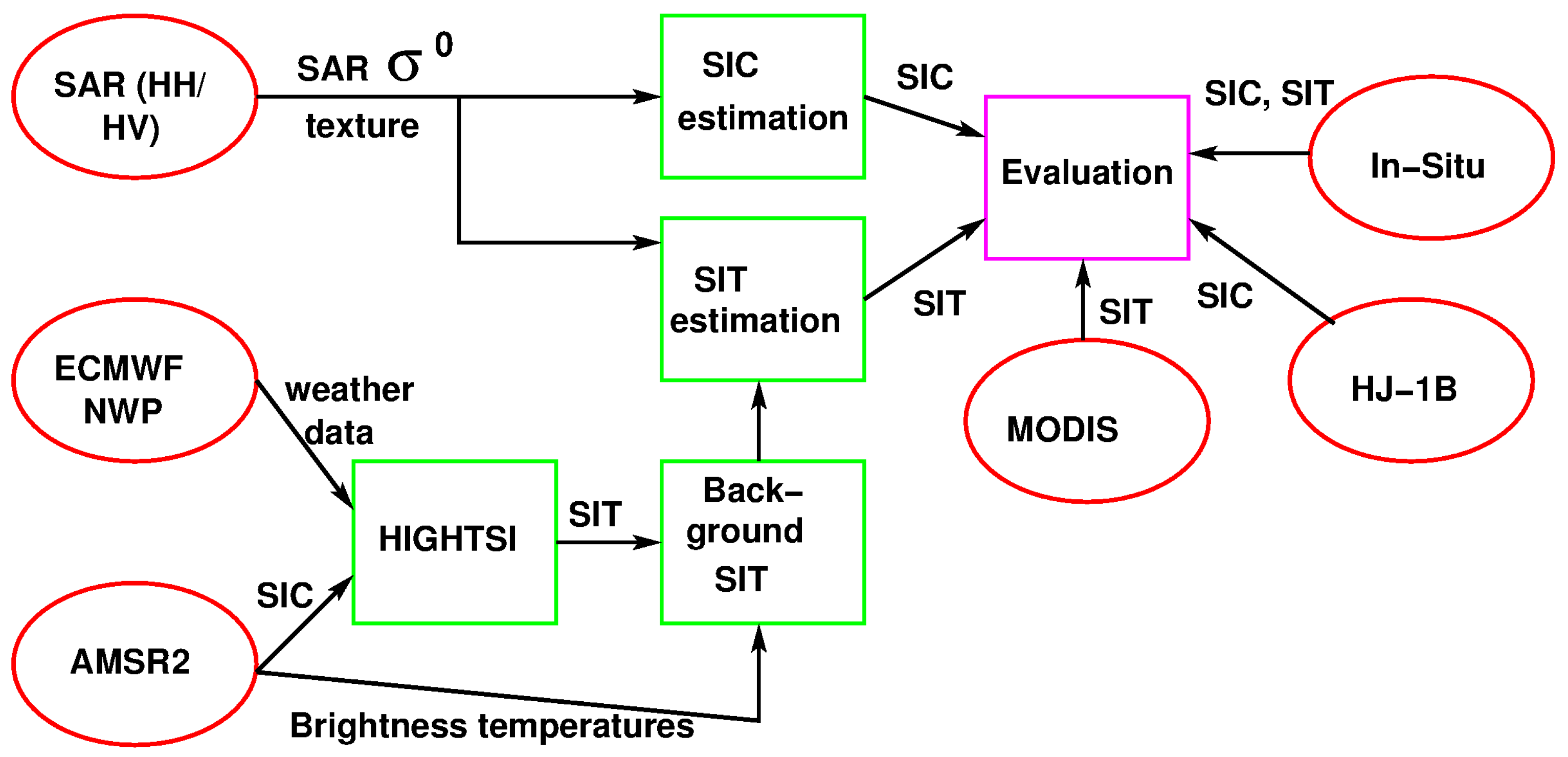
4. Estimation of Sea Ice Concentration and Thickness

Here, the developed SIC and SIT retrieval methods for the RS-2 SCW dual-polarized SAR imagery are presented. The SIC estimation methods were developed using either the in-situ data or the MODIS SIC data as a reference. The SIT estimation is based on a modification of the background SIT field derived from the AMSR2 and HIGHTSI data, with SAR backscatter statistics.

The estimation results were evaluated by dividing the in-situ data sets into training and test data sets—both representing about half of the available measurements—and evaluating the algorithm results using the independent test data set. The SIC estimates were also compared to the SIC estimates from the MODIS and HJ-1B imagery over the cloud-free areas. The SIT estimates were also qualitatively and visually compared to one MODIS SIT product.

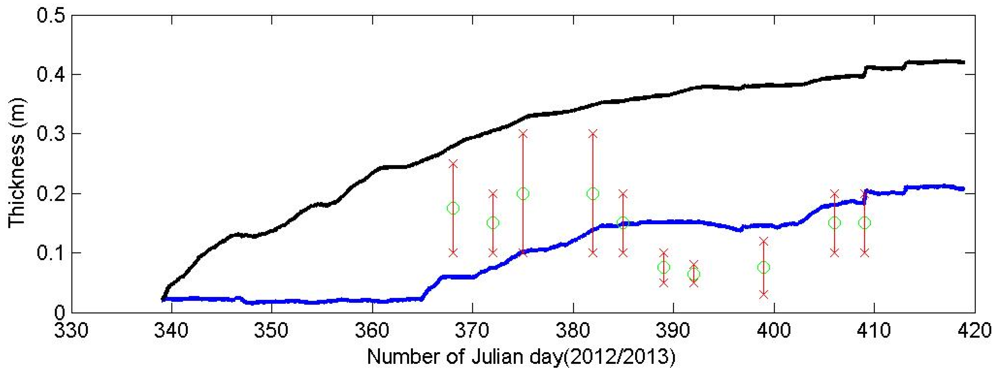
4.1. Background Ice Thickness Fields Based on HIGHTSI and AMSR2 Radiometer Data

The background ice thickness ($h_B$ in cm) was estimated using the HIGHTSI model and AMSR2 radiometer data, which were both interpolated to 1 km pixel size.

As described in Section 3.6, the thermodynamic sea ice growth for the Bohai Sea is modeled using HIGHTSI. The deficiency associated with HIGHTSI is that it is a 1-D model, and ice drift is only taken into account by assimilating SIC information. Hence, the local-scale spatial distribution of SIT is often inadequately described by the model. This explains, for example, the negligible correlation between the in-situ and HIGHTSI SIT ($r=0.1$). To put this result in perspective, we must consider that the atmospheric forcing for HIGHTSI is given on a spatial scale of tens of kilometers, whereas point-wise in-situ measurements are taken on scales of up to a few hundred meters only. However, earlier studies [69] demonstrated that the HIGHTSI model is capable of estimating the thermodynamic growth of sea ice with reasonable accuracy. Hence, we assumed that the HIGHTSI results for the total ice growth in the Bohai Sea could be used as an approximation for the total ice volume ($V_i$) increase in the area. The uncertainty of the HIGHTSI estimate for $V_i$ is unknown.

Here, the AMSR2 data were used to improve the description of the spatial distribution of $V_i$ in the $h_B$ grid. In our earlier study [37] for thin-ice detection in the Kara and Barents Seas, a linear combination of GR8936H (GR) and PR36 (PR) were mostly able to discriminate between thin-ice (<30 cm) and thick ice (>30 cm) areas in cold conditions. The LDA scores $s=a\times GR+b\times PR+c$ were used in the classification between the ice classes of thicker ($h_T>30$ cm) and thinner ($h_T<30$ cm) ice. The thickness values $h_T$ refer to the MODIS-based SIT, which were calculated according to the algorithm in [40]. We note that the weighting parameters $(a,b,c)$ of the GR and PR statistics were determined by the linear discriminant analysis (LDA) and were dependent on sea ice surface properties—among others, the surface temperature. In [37], the reference data set consisted of $h_T$ thickness values, which were mostly computed when the air temperature $T_a$ was below $-25{}^{°}$C in the Kara and Barents Seas.

In the Liaodong Bay, $T_a$ is in general much higher than in the Kara and Barents Seas. Therefore, we cannot use the LDA score parametrization from our earlier study [37] for the Bohai Sea. Due to lack of MODIS SIT charts over the Bohai Sea, we extracted a sub-set of $h_T$ and (GR,PR) pairs for warmer conditions with $T_a$ above −20 ${}^{°}$C over the Barents and Kara Seas. This Arctic data set contained 11,363 thin-ice samples with $h_T<30$ cm and 1641 samples with $h_T>30$ cm. The LDA score parameters were calculated as in [37], and they are $(a,b,c)=(33.72,38.54,-1.14)$. The whole Arctic data set is referred to with $A=(h_T,s)$. The difference to [37] is that now PR has a slightly larger weight than GR, but in [37], the weight of GR was about twice of that of PR. There were also other sources of uncertainties for the LDA approach, e.g., the (GR,PR)-distributions for the two ice classes are only roughly Gaussian, whereas the LDA assumes that they are exactly Gaussian.

To inspect the relationship between $h_T$ and the LDA scores s, we extracted from A those observations which fulfilled two criteria: (i) the $h_T$ value was below 30 cm and (ii) the corresponding s value was positive. The $h_T$ limit was set to 30 cm because it was the largest thickness value in our in-situ data set. The restriction to only positive s values was done because only positive s values occurred in the Liaodong Bay. As in the Arctic seas, negative s values were also obtained for thin-ice; we can conclude that in the warmer conditions the LDA values are somewhat larger than in the cold Arctic conditions.

From each 10 cm thickness range (1–10 cm, 11–20 cm, 21–30 cm), we randomly sampled 1000 observations. Then, we fitted in the resulting $(s,h_T)$ set a nonparametric regression curve and its 99% confidence interval using the Loess method [78] (Figure 6).

It is evident that there exists a trend between s and $h_T$. When SIT increases, the LDA value on average decreases for thin-ice. The large dispersion around the regression curve indicates that it is not possible to predict SIT using only the LDA scores—the uncertainty is too large. Instead, s can be used as a crude indicator of SIT magnitude.

The following procedure to construct a weighting function for $h_B$ was used. On the basis of the observation that the Bohai Sea s values are generally larger than the Arctic ones, we determined the weight function so that for a fixed s the weight is close to the thickest $h_T$ value occurring in the Arctic data set. Hence, the weight value is also geophysically possible in the Arctic, although with a small likelihood. The weight function describes the relative thickness differences over the range of s.

The weight function w depending on s shown in Figure 6 is defined as follows:

$$\begin{array}{ccc}\hfill w(s)& =& 0.7\times (5.5-1)\times s+8,\mathrm{if}s\in [0,5.5]\hfill \\ & =& 5,\mathrm{if}s\in [5.5,7]\hfill \\ & =& 1,\mathrm{if}s\in [7,11].\hfill \end{array}$$

In Figure 6, the function $w(s)$ was drawn only from $s=0$ to $s=5.5$.

The weights were normalized to one over the whole ice cover. Applying these weights, we multiplied the total ice volume $V_i$ modeled by HIGHTSI. The result was the HIGHTSI/AMSR2 background field $h_B$.

To exemplify how the addition of the AMSR2 data changes the HIGHTSI field, we present a series of four different images in Figure 7.

We can see that the MODIS-based SIT chart agrees well with the HIGHTSI/AMSR2 background field. Additionally, the visual interpretation of SAR imagery supports the matching of these two SIT charts. In the HIGHTSI-based SIT chart, the thickest ice occurs at a different location than in other charts.

The impact of the addition of the AMSR2 data can also be seen in the correlation between $h_B$ and the in-situ measurements. The correlation coefficient r was around 0.5 in this data set ($n=27$), whereas it was close to zero between the HIGHTSI SIT values and the in-situ measurements. We excluded four in-situ measurements from the computations, which according to the SAR images were situated in open-water. The bootstrap-based 95% confidence interval for r was (0.25, 0.80) when bootstrapped 1000 times.

Considering that the LDA scores and the point-wise in-situ measurements were at highly different scales (≈100 km${}^2$ vs. 0.25 km${}^2$), we regard the $r=0.5$ value as acceptable. The SIT variation in 100 km${}^2$ area is so large that we cannot expect a very high correspondence between the point-wise in-situ measurements and the mean SIT over a large area. Additionally, the small sample size affected the r value and the width of its confidence interval.

The open-water area in the HIGHTSI SIT field was based on the ASI SIC product. In $h_B$, we used the same open-water areas as in the HIGHTSI model runs. Visually comparing the LDA s images to the SAR images, we noted that the values $s\in [7.11]$ usually indicated low SIC. Hence, a negligible weight was set for these s values.

The land spill effect (e.g., [79]) is present in the AMSR2 data. Based on a visual inspection, it affected the s values up to 4–5 km from the coast by reducing s and hence by increasing the estimated SIT near the coast. In the estimation of $h_B$, we have not explicitly taken this effect into account.

A simple approach to reducing the land spill effect would be to exclude the near-coast grid points (within a radius or 4–5 km) and then extrapolate the values in the coastal areas. This approach would just lead to a different kind of estimation errors. We also notice that the possible overestimation due to the land-spill effect is at least partially reversed by the SAR-based SIT estimation.

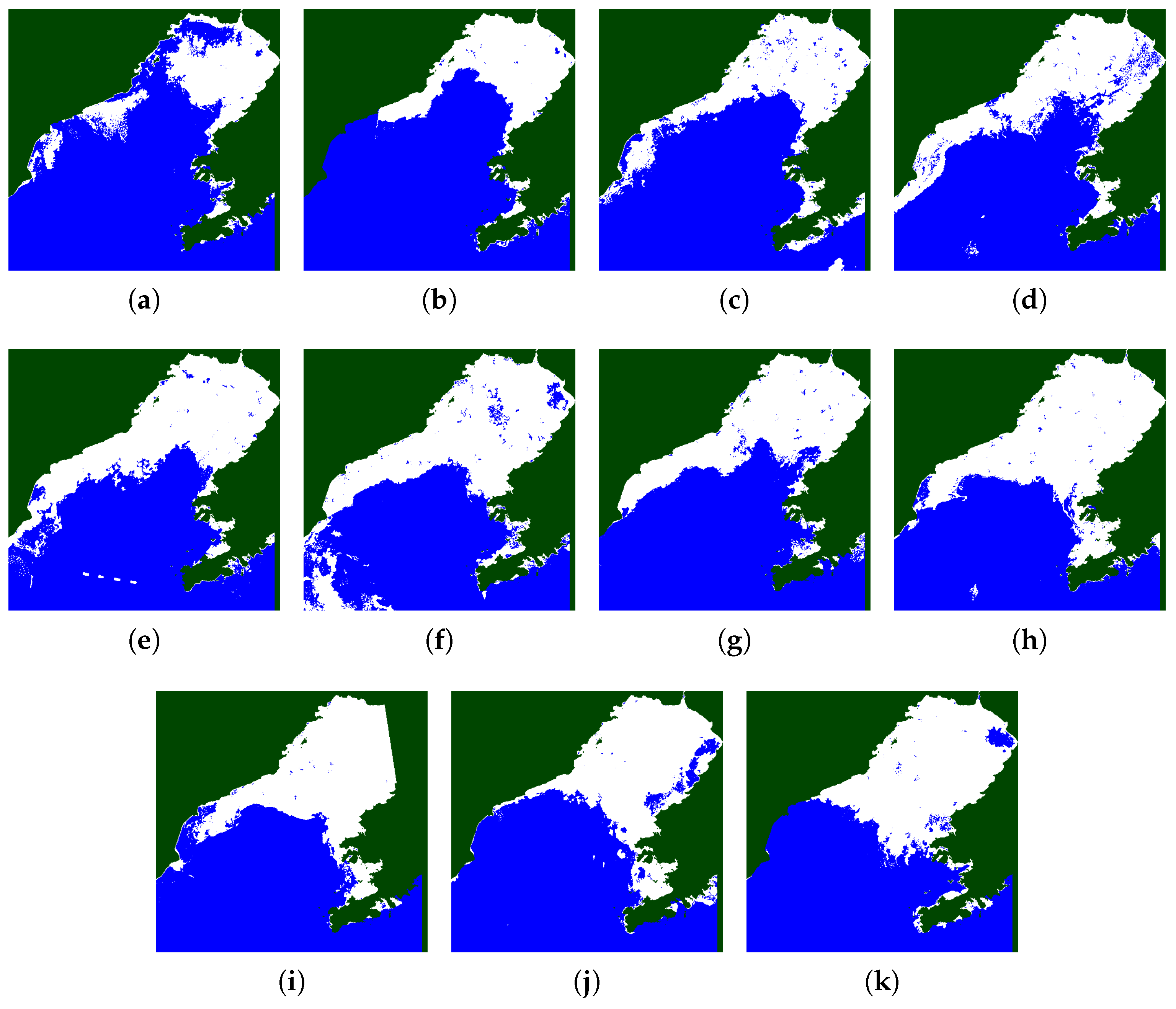
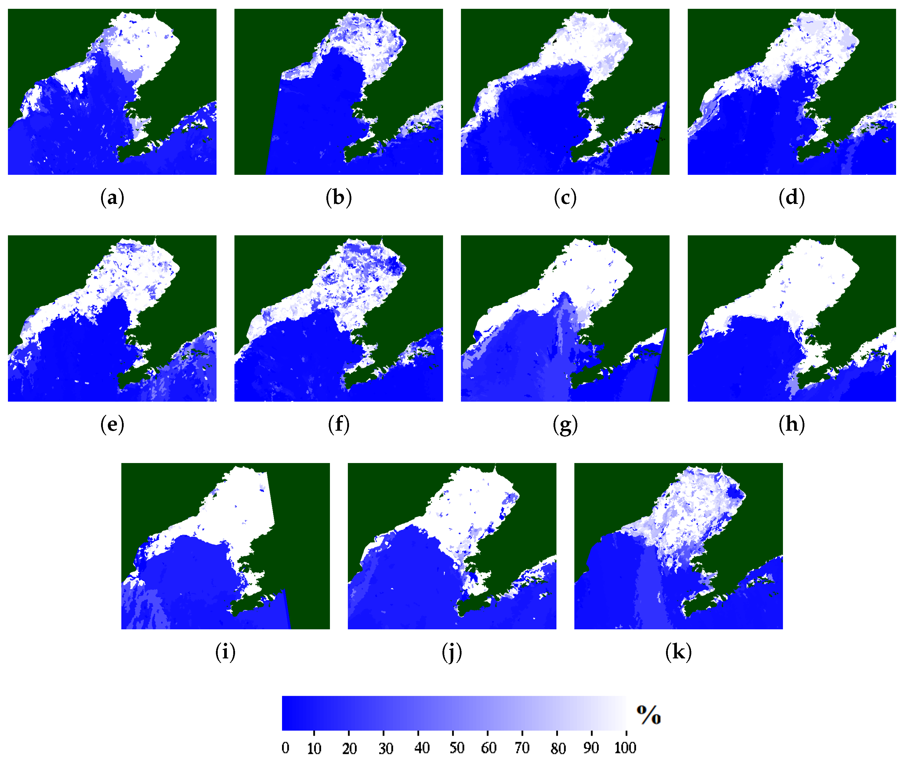
4.2. Sea Ice Concentration Estimation and Ice/Open-Water Discrimination Based on SAR Imagery

In the following, we first introduce a linear SIC estimation method defined as using in-situ SIC data as a reference, and then another nonlinear method using the MODIS SIC data as a reference. This is followed by a validation study. The RS-2 SAR imagery used in our experiments as thumbnail images are shown in Figure 8 (HH-channel) and Figure 9 (HV-channel).

4.2.1. Linear Model Between in-Situ SIC and SAR Data

We studied SIC estimation based on a linear model between the reference SIC data and segment-wise SAR backscatter and various textural features. The reference SIC data consisted of the in-situ data and also selected open-water points outside the ice-covered area; see Figure 4. A selection criterion for the open-water points was that they remained open throughout the study period. Original in-situ SIC data consisted of minimum and maximum data, which were averaged for the reference data. The reference SIC data were divided into training and test data. The training data consisted of 36 points (the open-water reference points were included), and the test data consisted of 35 points.

Sea ice and open-water were distinguished based on a linear regression (least squares fit) using the minimum sum of squared residuals as the feature selection criterion (i.e., selecting the $N_f$ features producing the smallest estimation error for a given number of the features $N_f$). It was possible to search through all the feature combinations for each $N_f$, because the amount of training data was so small.

Based on the training SIC data set, five features were found to be enough. These automatically selected features were $C_A^{HH}$, $E^{HH}$, $N_c^{HH}$, $V_1^{HV}$, and $V_2^{HV}$. The values of $R^2$ were 0.98 ($n=36$) and 0.97 ($n=35$) for the training and test data sets, respectively, and the corresponding absolute estimation error was five percentage points for both data sets.

The equation for the linear SIC (C) estimation was

$$C=a_c{f}_c+N(0,\sigma ),$$

(7)

where $a_c$ is the vector consisting of a set of linear coefficients and the feature vector $f_c=[C_A^{HH}{E}^{HH}{N}_c^{HH}{V}_1^{HV}{V}_2^{HV}1]$. The last value 1 in the feature vector $f_c$ corresponds to the constant (intercept) term. $N(0,{\sigma }^2)$ is a Gaussian error term with zero mean and with an unknown variance ${\sigma }^2$. The estimation results for the training and test data sets are shown in Figure 10, and the estimation results for all the SAR imagery are shown in Figure 11. Figure 10 indicates that the linear method gives good estimates for both training and test data sets for both high and low SIC values. In the left part of Figure 10a,b (representing open-water areas), we see that the estimated SIC for the open-water areas is 20% or less for both the training and test data sets.

As there were mostly high SIC values (close to 100%) in the training data set and on the other hand the open-water points (i.e., zero SIC values), the linear equation is not very accurate for estimation of the intermediate SICs. However, it is efficient for distinguishing between open-water and sea ice. This mask is applied to the SAR imagery before the SIT estimation. The SIC threshold for distinguishing between open-water and sea ice applied here was 50%. The resulting masks are depicted in Figure 12.

4.2.2. SIC Estimation with a Neural Network Approach

We also studied a nonlinear method for the SIC estimation. The nonlinear approach utilizes Multi-Layer Perceptron (MLP) neural networks [80]. The amount of in-situ measurements was not large enough for the MLP training, and thus the MODIS open-water/ice classification was used to derive segment-wise (corresponding to SAR segments) SIC estimates to be used as the training data set for the MLP approach. An MLP with 20 nonlinear hidden layer neurons was applied, and the same five SAR features as those selected in the linear estimation were applied to estimate SIC. Four SAR images were selected for training and three for testing, and the MODIS SIC segment medians (corresponding to SAR segmentation) as the target were used. The features were medians over the SAR segments, and the MODIS SIC was estimated by counting the ratio of open-water pixels to the number of all the pixels within each SAR segment. The estimation results are presented in

Table 3. Multi-Layer Perceptron (MLP) ice concentration estimation results compared to the MODIS estimates. The values are given in percentage points. MSE: mean squared error.

Data Set	Bias	Absolute Error	MSE	R${}^2$
train	10.8	17.6	28.2	0.64
test	−0.65	15.7	26.9	0.64

, and the corresponding SIC estimate images are shown in Figure 13. For the training data set, there was a bias of over 10 percentage points (indicating overestimation), which was not the case for the test data set. This was a surprising result, indicating that the training data set likely included some contradictory samples. These contradictory samples are likely to be produced by the time differences between the reference data set and the SAR data set and ice drift between their acquisitions. The computed absolute error of 17.6 percentage points (training data set) and 15.7 percentage points (test data set), the mean-square-errors of 28.3 and 26.9 percentage points, and $R^2$ of 0.64 for both the data sets indicate that SIC can be rather well estimated for the data sets (even when the training data set may include some inconsistent data), although it naturally needs to include enough (a dominant portion) consistent data. There were more values of the lower and higher ends of the SIC distribution present in the training data. The proportion of open-water input vectors was 15.1%, and the proportion of the inputs with SIC values in the range of 0–10% (including open water) was 33.9%. In the upper end, the proportion of the input values with SIC in the range of 90–100% was 20.4% and the proportions of the input values with SIC range 80–90%, 70–80% and 60–70% were 9.1%, 9.7%, and 8.1%, respectively. The proportions for the other ten percent ranges were from 1.6% to 5.4%, indicating that the proportion for the SIC range 20–60% is clearly under-represented in the data. This can affect the estimation accuracy of the mid-range SIC values.

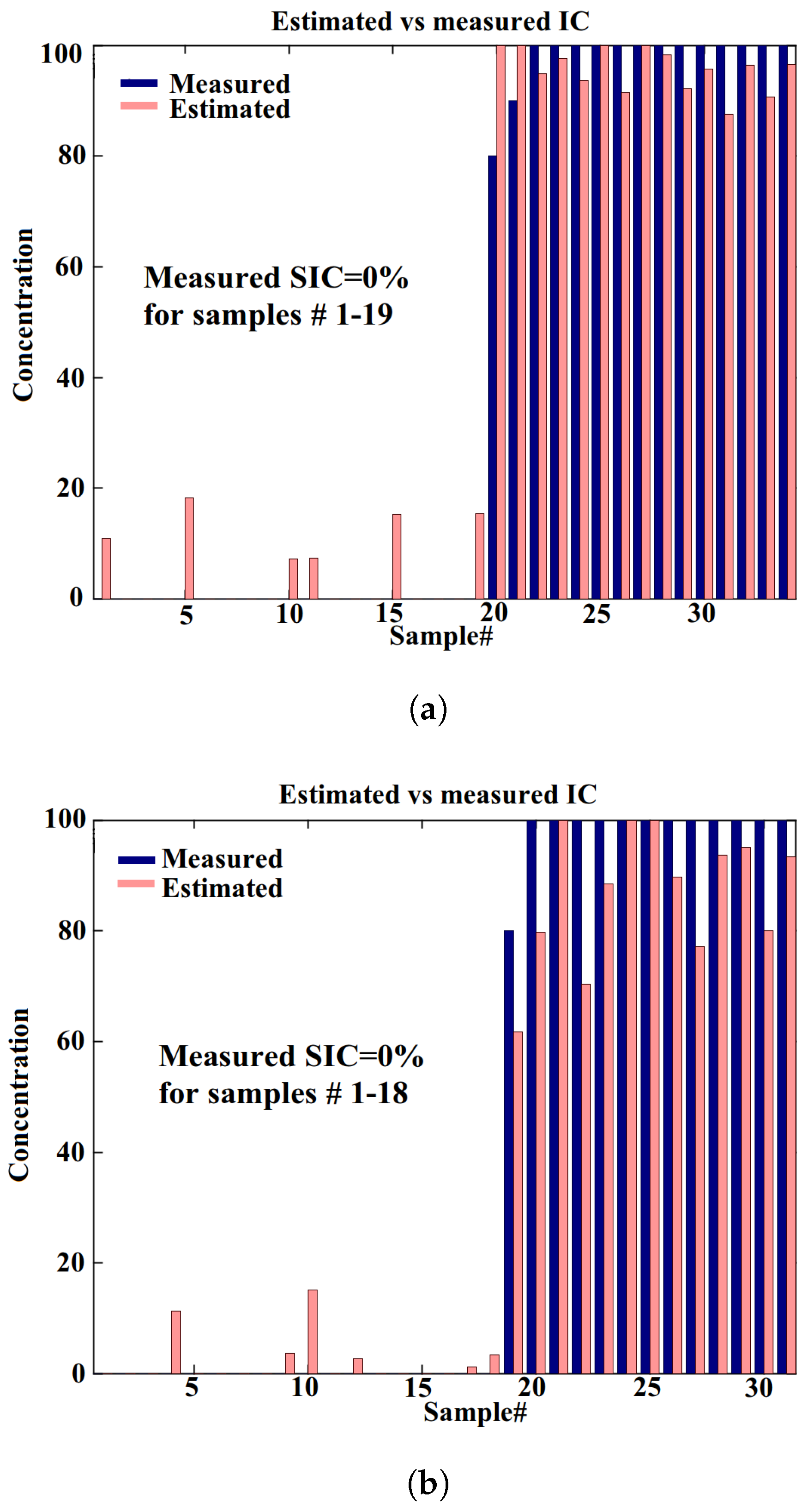
4.2.3. Evaluation of the SIC Estimates

The SAR-based SIC estimates were compared to the SAR segment-wise SIC computed from open-water/sea ice classification based on the HJ-1B (9 January 2013) optical image. The SIC estimates for HJ-1B and SAR are presented in Figure 14. The evaluation was performed by randomly sampling a total of $n=10,000$ grid points (higher N did not change the evaluation statistics) in a resolution of 500 m. $R^2$ between the HJ-1B and SAR-based SIC estimates were 0.65 ($n=10,000$) for the linear model and 0.71 ( $n=10,000$) for the MLP model. The $R^2$ values for this larger data set were significantly smaller than those for the small test data with the linear model. In Figure 14, we can see that the linear method seems to overestimate SIC near the ice edge, and in some high-SIC areas underestimates SIC with respect to the HJ-1B estimates. The MLP method seems to overestimate SIC in the areas of mid-range SIC, but large sea ice areas with SIC close to 100% and larger open-water are well distinguished. The differences between the SIC estimates can partly be explained by the different resolutions of the data sets and partly by the fact that the restricted (not totally representative) training data sets for both the linear and MLP approaches contributed to the increased differences.

The SAR segment-wise SIC estimates differ from the MODIS and HJ-1B estimates, and indeed in some areas SAR seems to overestimate SIC. Additionally, the SAR SIC estimates (linear method and MLP) differ from each other. Better estimates could possibly be extracted by combining these methods, but as the reference data are also based on the EO data with their own uncertainties, evaluation of the real quality of the methods is difficult.

Some of the differences are also due to the time differences between the data acquisitions (they were just restricted to be made during the same day), and also misclassification of thin-ice to open-water or vice versa by either of the methods.

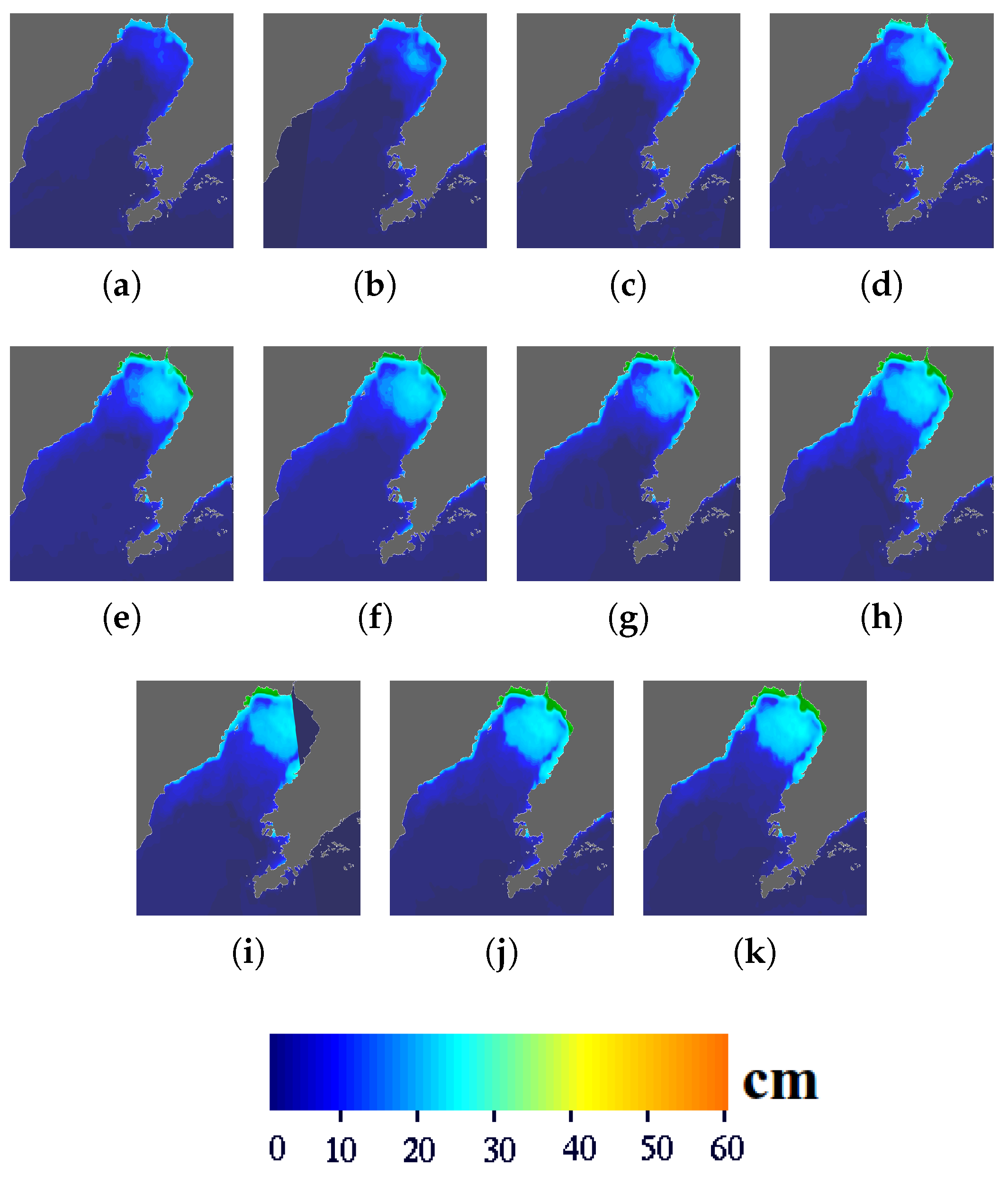
4.3. Ice Thickness Estimation Based on the Background Field and SAR

Ice thickness estimation was performed using a linear model including the background SIT field $h_B$ and SAR-based features. For training and testing purposes, the in-situ SIT data (see Table 2) was divided into training and test data sets. The training data set consisted of 14 measurements, and the size of the test data set was also 14 measurements. The estimation was made for the area with SIC larger than 50% (linear SAR SIC estimation). The in-situ measurements consisted of the SIT range, and the average SIT (the average of the lower and upper bounds of the SIT range).

Selection of the SAR features was done by minimizing the squared sum of residuals of a least squares (LS) linear fit for the training data set; i.e., selecting the features minimizing the estimation error in a similar manner as for the SIC data. The estimation model used here was a linear model that included a modulation term between $h_B$ and each feature; i.e., SIT estimates H were of the form

$$H=\sum _{i=1}^{N_f}[a_i{f}_i+b_i{(f_i{h}_B)}^{1/2}]+c,$$

(8)

where $a_i$, $b_i$ and c are defined by the linear least squares fit, $f_i$ are the $N_f$ selected features.

The best results using the Liaodong Bay data set were achieved using only one automatically selected feature: the scaled entropy $E^{HV}$. The most significant term for this case was the cross-product term between $E^{HV}$ and $h_B$. For $E^{HV}$, the coefficient $b_1$ of this term was approximately 0.3, and the value of $a_1$ was in practice negligible (≈−0.0038). The results for this selection are shown in Figure 15. The value of $R^2$ for the training and test data sets was 0.71 ($n=14$) and 0.74 ($n=14$), respectively. Even though the number of samples n is so small, the linear dependence is statistically significant, as the Pearson correlation $R=0.86$ and $R^2=0.74$ are so high. Adding more features improved the estimation accuracy for the training data set as expected, but the estimation accuracy for the test data set then became worse. The results for up to three features are shown in

Table 4. Sea ice thickness estimation errors.

Features: ${\mathit{E}}_{\mathit{HV}}$
Set	Bias (cm)	Abs. Error (cm)	MSE (cm)	R${}^{\mathbf{2}}$
Train	0.25	2.89	4.13	0.71
Test	−1.21	3.53	4.17	0.74
Features: ${\mathit{E}}_{\mathit{HV}}$, ${\mathit{C}}_{\mathit{c}}$
Train	0.08	2.39	3.48	0.79
Test	−2.97	4.08	5.27	0.62
Features: ${\mathit{\sigma }}_{\mathit{HV}}^{\mathbf{0}}$${\mathit{E}}_{\mathit{HV}}$, ${\mathit{C}}_{\mathit{A}}^{\mathit{HH}}$
Train	0.11	2.35	2.98	0.85
Test	−0.72	3.74	4.72	0.57

. In order to better evaluate the estimation error, we undertook a cross-validation approach: we made a leave-one-out experiment (i.e., using all the SIT samples except one for training and the one sample left out for testing, then repeating the leaving out for all the samples) using the one and three-feature setups selected automatically. The results of the leave-one-out experiments are shown in Figure 16. In this case, the one feature model also gave the best SIT estimation result (RMSE = 4.5 cm); the three-feature case RMSE was 6 cm. This probably indicates that our data set was not fully representative due to its limited size, but some conclusions of the method’s performances can still be made based on this data set and the auxiliary EO data sets.

The modeled SIT by HIGHTSI for all of the studied SAR images are shown in Figure 17, the $h_B$ images (from the MODIS and AMSR2 data) are shown in Figure 18, and the SAR-based SIT estimates are shown in Figure 19. In this experiment, SIT was only estimated for the areas not classified as open water based on the linear SIC estimation and thresholding illustrated in Figure 12.

The HIGHTSI and the background SIT fields in Figure 17 and Figure 18 offer a general view of the ice development, but by only including the SAR data, there is a more realistic and detailed spatial distribution of SIT (Figure 19). As the SAR SIT charts include information on thin and thick ice in a high spatial resolution, they are useful, for example, in terms of ship navigation.

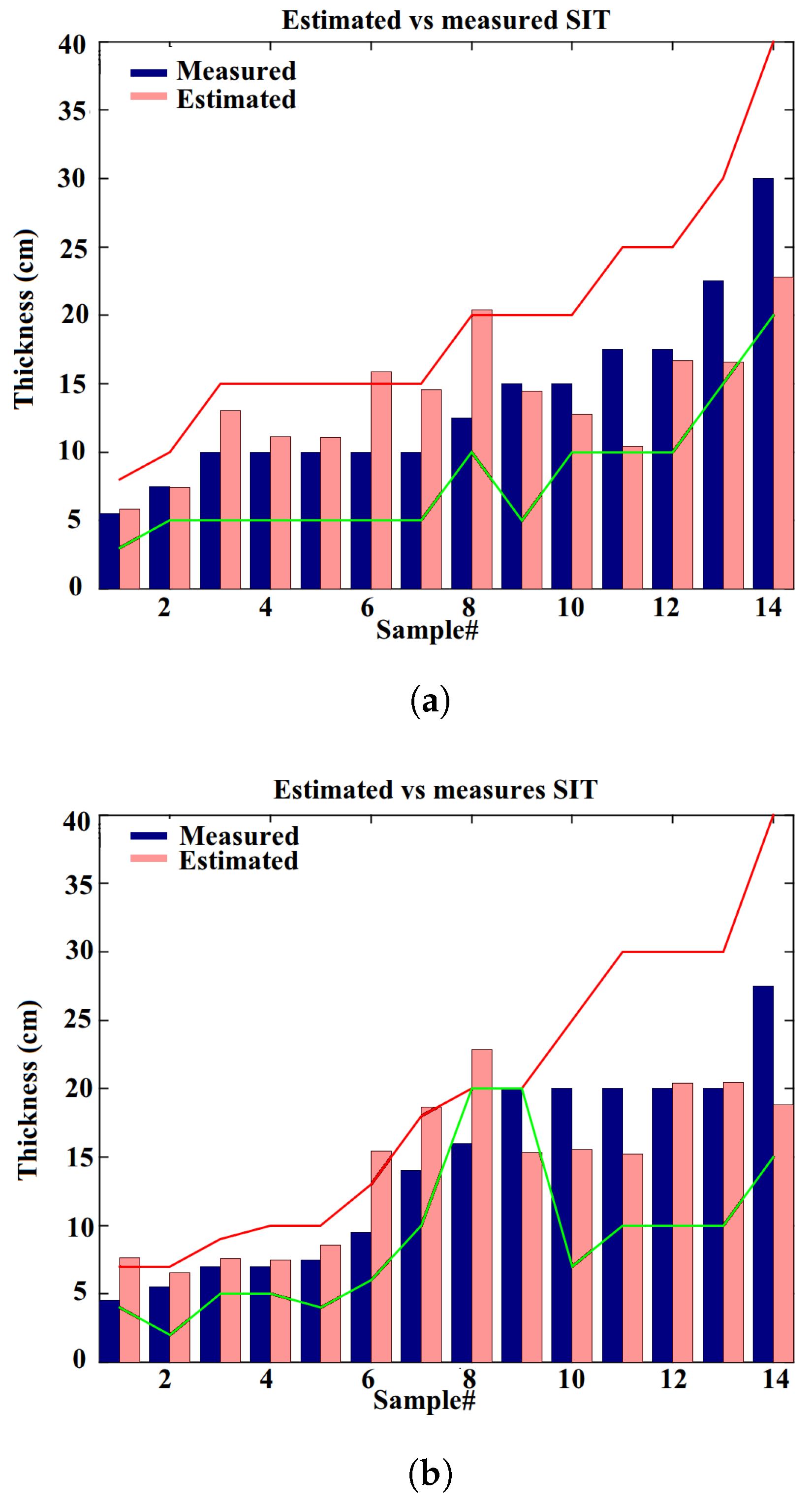
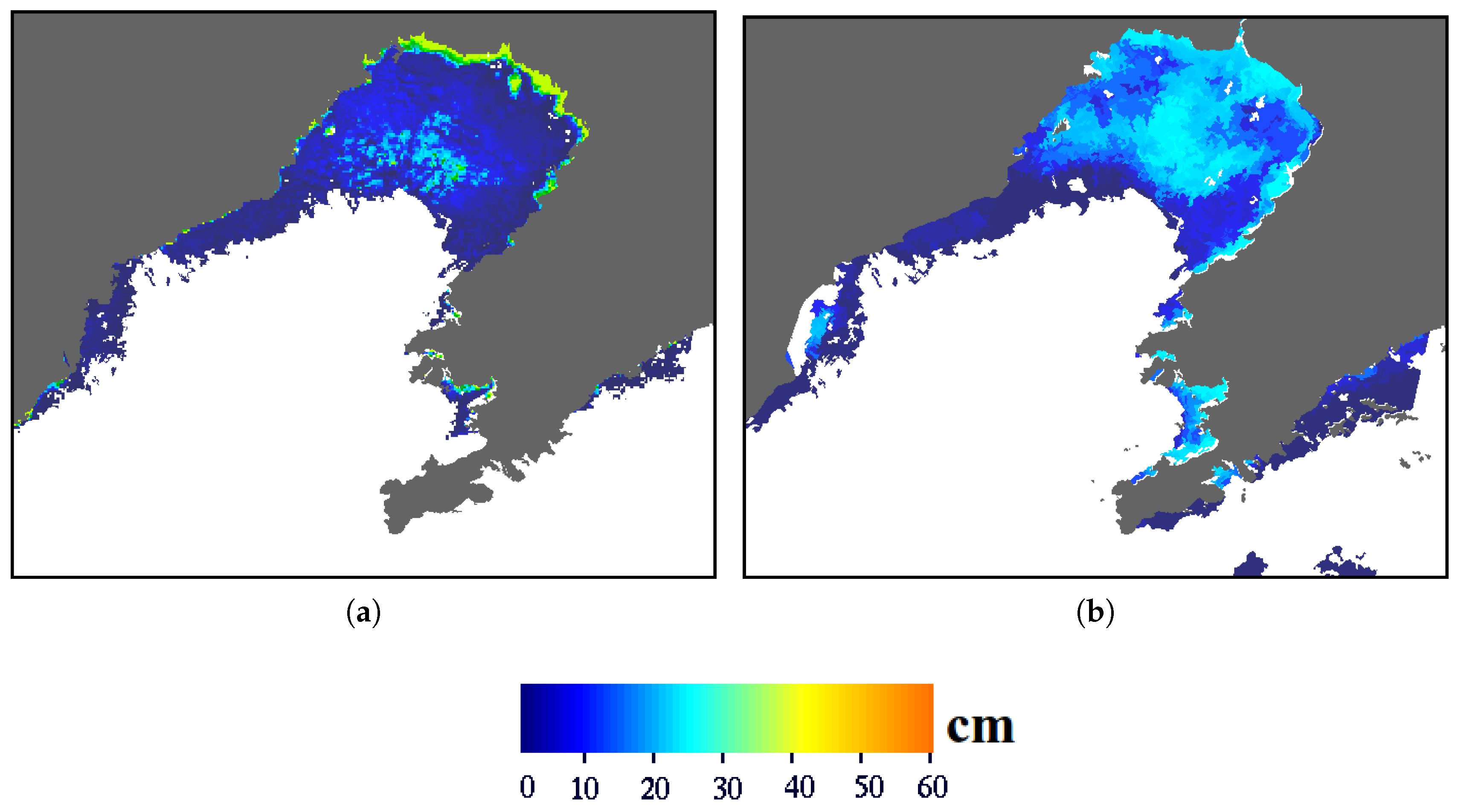
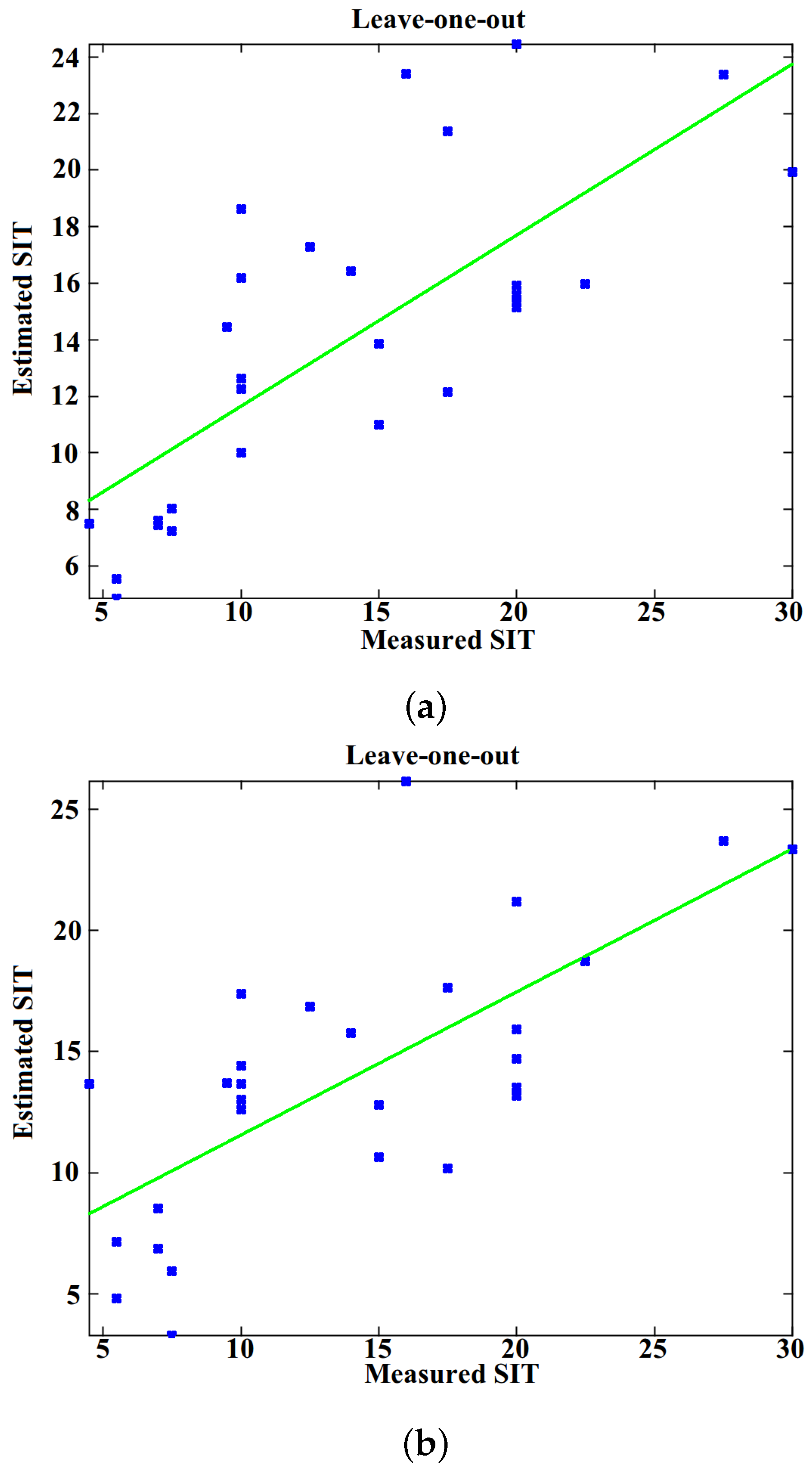
Evaluation of the SIT Estimates Using MODIS SIT

We had four MODIS SIT products at our disposal and we studied the use of them in the evaluation of our SIT estimates. The average difference between the SAR SIT and MODIS SIT was about 5 cm for cold days (9 January and 16 January 2013) and over 10 cm for the other two cases (12 February and 19 February 2013). The MODIS-based ice thickness for the Bohai Sea is sensitive to the changes of air temperature and only works reliably in cold air and ice surface conditions—presumably, $T_a$ below −10 ${}^{°}$C [41]. There was also approximately a 9 h time difference between the acquisitions of the MODIS and RS-2 imagery.

Therefore, we only made and show a comparison with one MODIS SIT product in Figure 20, 9 January 2013 (with cloudless weather conditions over most of the study area) and relatively cold weather conditions ($T_a$ was approximately −9 ${}^{°}$C). The MODIS SIT in general was thinner compared with SAR SIT in a large part of the Liaodong Bay. In the northern coast, MODIS SIT was certainly overestimated (50 cm), because the in situ observed ice thickness near the coast was typically 20–30 cm (Yu Liu, personal communication), very close to the SAR SIT product shown in Figure 20b. Due to the dynamic nature of the Bohai Sea ice and the time differences between the in-situ and SAR data, the estimation error increases because of temporal variations. This situation also applies to the time gaps between EO data acquired at different times, as we here only required that they are from the same day. Additionally, the different resolutions of the EO instruments contributed to comparison errors. Considering these potential error sources, we suggest that our new SIT estimation method is feasible for the Bohai Sea, but further validation with more MODIS SIT charts and other auxiliary SIT data would be desirable.

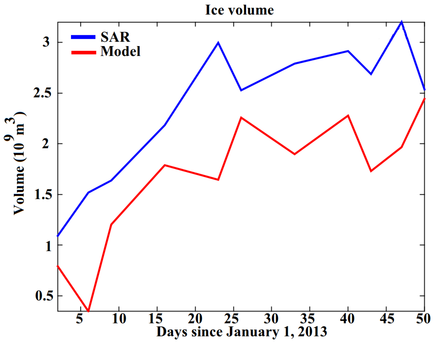
5. Bohai Sea Ice Volume

We also estimated the ice volume $V_{ice}$ for the study area based on the computed SIC (linear method) and SIT estimates C and H. This estimation was performed for the dates of the existing SAR data. The estimate for $V_{ice}$ was computed as

$$V_{ice}=A_p\sum _{(r,c)\in W}C(r,c)H(r,c),$$

(9)

where $A_p$ is one product grid cell (pixel) area (0.25 km${}^2$). The study area is denoted by W. In Figure 21, the estimated ice volume of the study area is based on the SIT and SIC estimates (linear method), and for comparison we have provided a $V_{ice}$ estimate using the HIGHTSI model and a SIC based on the National Snow and Ice Data Center (NSIDC) bootstrap algorithm [6,81] and the AMSR2 data. We used the bootstrap SIC algorithm because we specifically wanted to perform the comparison with $V_{ice}$ based on the thermodynamic evolution and with an independent SIC estimate (AMSR2 data is not used in our SIC estimation, it is used only in the SIT estimation). Actually, the SAR based SIC in combination with HIGHTSI produced very similar results. $V_{ice}$ has been computed over the common area of all the available SAR images. Both the SAR- and HIGHTSI model-based ice volumes were in a growing phase in January and February. The trends for January are quite the same, because the ice growth in January was rapid. Thermodynamics gave a major contribution to the increase of the total $V_{ice}$. From late January onward, the increase of $V_{ice}$ was slowing down, and the temporal differences between the SAR and model-based $V_{ice}$ grew. The ice extent often reaches its maximum in early February when SIT reaches its thermal equilibrium stage, and the convergence/divergence due to ice motion (such as ice drift) and internal stress tend to dominate the spatial and temporal variation of the total ice volume.

6. Discussion

We performed a study of sea ice concentration (SIC) and sea ice thickness (SIT) estimation based on a sea ice model, RS-2 SAR and AMSR2 microwave radiometer data in the Bohai Sea during the 2013 ice season (January–February). The northern Bohai Sea has a seasonal sea ice cover, but a typical ice season is relatively short—only a few months. However, as marine transportation and offshore activities (e.g., oil exploration and drilling) continue, exact knowledge of the prevailing ice conditions is crucial. Additionally, we used available in-situ data measured on the oil platforms in the study area and auxiliary EO data to train and evaluate the developed algorithms. Unfortunately, our available in-situ data set was relatively small, but we were still able to demonstrate the potential of the studied methods for high-resolution SIC and SIT estimation over the Bohai Sea. The in-situ measurements were not exactly compatible in time with the RS-2 SAR imagery used. As Bohai Sea ice is dynamic, it also made its contribution to the SIC and SIT estimation accuracy when comparing the estimates with the in-situ measurements of the training and test data sets. Against this background, we can consider our results good. The absolute error for the SIC estimates were about five percentage points for the linear estimation method for both training and test data sets. The absolute error for the nonlinear Multi-Layer-Perceptron (MLP) neural network SIC estimate was higher, at around 15 percentage points. This larger error of the MLP method can partially be explained by the different acquisition times for the MODIS SIC data used as reference and the RS-2 SAR imagery and the ice drift between the acquisition times. The training SIC data set was not representative in this case. In some cases, the SIC estimates were better for the test data set than for the training data set. This issue can also be explained by inconsistencies due to the ice drift. Exact coincidental in-situ and SAR data would likely have given better estimation accuracies. The absolute error for the linear SIT estimates was around 3 cm, which can be considered a good result even for thin seasonal sea ice.

For operational SIC estimation, the available algorithms are mainly based on microwave radiometers [6,7], with a coarse resolution of several kilometers. High-resolution SIC estimates based on SAR backscatter and SAR texture measures were presented earlier (e.g., in [9,10,11,12,13,14,15,16,17]). However, these methods have different performances in different conditions. To be able to reliably estimate (especially the intermediate SIC values), a large training data set that includes SIC values over the whole SIC range from low to intermediate and further to high SIC, would be needed. In typically available SIC training data sets such as digitized ice charts, there exist more SIC values near to 100% or 0% than values in the SIC mid-range (roughly 20–80%). This circumstance was the case for our in-situ SIC data as well. Because of the restricted amount of the SIC in-situ data, we studied here a rather simple linear model to estimate SIC, and concluded that we reached a good discrimination between open-water and sea ice classes based solely on the SAR data. Due to a lack of suitable in-situ SIC data, a rigorous evaluation in the intermediate SIC value range was not possible. Classification into open-water and sea ice classes based on SIC thresholding was then used as an input for the SIT estimation algorithm (i.e., SIT was estimated for the sea ice class only). For this purpose, the obtained high-resolution SIC estimates proved to be both useful and reliable. In conditions of somewhat thicker seasonal sea ice, (e.g., in the Baltic Sea), the SAR-based SIC estimates seemed to have a smaller estimation error [16,17]. This result may have been due to the fact that for the Baltic Sea there was very good SIC data from the digitized Finnish ice charts available for the SIC algorithm training and evaluation.

SIT estimation for the Bohai Sea from SAR data seems to be feasible, even with a relatively straightforward empirical relationship between the SIT and SAR data [47,82]. However, defining this relationship would require an extensive in-situ data set on SIT or the ice surface topography. In [82], the relationship between Bohai Sea deformed sea ice thickness and the C-band ${\sigma }_{VV}^0$ was defined only for one SAR image, resulting in a good fit ($R^2\approx$ 0.9, $n=65$). Level-ice thickness was defined based on the visible/near-infrared (VIS/NIR) reflectance imagery. Another practical problem for using VIS/NIR imagery is that they require cloud-free conditions and solar illumination. As we were using only microwave data, neither was required.

However, studies conducted in other sea areas with seasonal sea ice [14,52,54] do show that the relationship between C-band or X-band SAR ${\sigma }^0$ and SIT is not that straightforward, but rather depends on several factors, such as the imaging geometry (local incidence angle), wetness of the surface, and overlaying snow cover properties. Co-polarized backscattering from open-water—and also from leads and cracks—varies a lot depending on the wave conditions in the open-water (high backscattering from open-water can be caused by waves through Bragg scattering). Open-water can thus produce similar backscattering as different ice surfaces, leading to various erroneous SIT estimates over the open-water. Cross-polarized backscattering does not have this property, and it is typically low for open-water, but it is also low for level-ice and even for ice with some minor deformations. We have included the SAR texture features computed for both co-polarized and cross-polarized channels in our estimation method to overcome the problems related to using backscattering directly. Utilization of the SAR co-polarization ratio has been shown to be a promising quantity for SIT estimation [49,83], but both co-polarized channels are not available in the current operational SAR modes; they are available only in polarimetric modes, which cover areas too small for operational sea ice monitoring. In the near future, this situation will be improved when SAR instruments with a circular polarimetric (compact polarimetry) mode—such as the Canadian RADARSAT Constellation Mission—are available.

The most promising approach for the C-band SAR based SIT estimation using the currently available wide swath SAR data suitable for operational sea ice monitoring is probably the approach wherein a background SIT field is refined into a finer resolution based on automated SAR image analysis utilizing the level of ${\sigma }^0$ and the texture features derived from the spatial variations of ${\sigma }^0$. This approach can be complemented by microwave radiometer data to improve the detection of thin-ice areas. Such approaches have been proposed, for example, in [53,54,55,56]. The method developed here is a variant of this approach, combining a background SIT field from an ice model and microwave radiometer data and SAR backscattering and texture features for a fine-resolution SIT estimation.

Radar altimetry [34,35,36] is not suitable for a high-resolution SIT estimation of relatively thin sea ice. The SIT estimates based on radar altimetry, such as CryoSat-2, include many uncertainties, especially in the freeboard-to-thickness conversion [84], which typically contributes more to the SIT estimate than does the typical ice thickness in the Bohai Sea.

We used one MODIS SIT chart during a cold period for a qualitative comparison between the MODIS SIT chart and our new SAR-based SIT chart for the same day. On the basis of this limited data set, the comparative results suggest that our SAR-based method seems to somewhat overestimate SIT compared to the MODIS SIT in the Liaodong bay. However, in the coastal zone, there was underestimation. In general, the two methods yielded mutually similar estimates for the areas of thinner and thicker ice.

7. Conclusions

We studied sea ice concentration (SIC) and sea ice thickness (SIT) estimation for the Bohai Sea during the winter 2012–13 using RS-2 dual-polarized SAR imagery, AMRS2 radiometer data, and SIT data based on the thermodynamic sea ice model HIGHTSI. The advantage of using SAR and AMSR2 is that SIT can be estimated even during cloudy periods and without daylight illumination. The SIC and SIT estimation methods were developed and validated using in-situ data, SIC and SIT charts from the MODIS imagery (SIC,SIT), and the HJ-1B spectrometer (SIC) imagery. The available in-situ data sets were relatively small, but nevertheless we were able to demonstrate the potential of dual-polarized C-band SAR data in estimating the Bohai Sea SIC and SIT.

The SIC estimation results suggested that ice and open-water discrimination works well using a simple linear SIC model that has various SAR textural features as input. We also tested a nonlinear approach based on the MLP neural network for the SAR-based SIC estimation using MODIS open-water-sea ice charts as the reference data. In the MLP method, exactly the same set of SAR features were used as in the linear SIC estimation method. The MLP results were not as good as the results of the linear method, but this may be because the training and test data sets were not exactly coincident, and some ice drift between the acquisitions of the different data sets probably occurred. The reference SIC estimates were also based on another EO data set (HJ-1B), and the training and test data sets were larger than our very limited in-situ data set. Yet still, the SIC data sets were not representative; i.e., they were not covering all kinds of variations of the SIC range. These are all factors that affect the SIC estimation process and its quality. We can conclude, however, that SAR SIC estimates can be used to distinguish between ice-covered and open-water areas in most cases in the Bohai Sea. Both tested methods followed by thresholding offer a useful classification for sea ice and open water classes, but in this case, the linear method seemed to work slightly better. The SIC estimation can be improved by using a larger and more comprehensive and timely (coincident training and test data sets) training data set.

For the further development of the SIT estimation method, the number of in-situ measurements was restricted, but it was still possible to set up a linear SIT estimation model and test it based on the data set. We were able to extract and demonstrate useful SIT estimates using a leave-one-out approach. However, nonlinear complex estimation approaches, such as the MLP approach, cannot be established with such a small amount of (training) data.

A major factor affecting the evaluation results here was that the in-situ measurements and SAR data were not acquired simultaneously. There were time differences of up to a day, and the relatively thin Bohai Sea ice is also highly dynamic by the nature. The temporal differences between the reference data sets (in-situ data used in training and testing) and the remote sensing data were also the reason for occasional inconsistencies between the data sets used for training and testing the algorithms, and explain the cases where the results were even better for the test data set than for the training data set. This result indicated more inconsistency in the corresponding randomly selected training data set than in the test data set. Simultaneous in-situ measurements and SAR data would likely have led to better estimation results, especially for SIT.

In any case, the results obtained were promising, and operational ice monitoring based on the studied methods does seem possible. The proposed methods can provide SIC and SIT estimates in a very high resolution, independently of cloud cover and solar illumination, thus enabling operational sea ice monitoring in all conditions. Additionally, ice volume from a basin scale to local scales can be derived from the high-resolution SIC and SIT estimates in a straightforward manner. This study also offers guidelines for implementing high-resolution SIC and SIT estimation and monitoring in the Bohai Sea and other similar semi-enclosed sea (or large lake) areas that have a seasonal sea ice cover. However, a much larger and more representative training data set that describes all possible ice conditions in an area will be required to set up a reliable operational SIC and SIT estimation system when utilizing the proposed methodology.

References

1. Bai, S.; Liu, Q.; Hai, H.L. Sea ice in the Bohai Sea of China. Mar. Forecast 1999, 16, 1–9. (In Chinese) [Google Scholar]
2. Li, Z.; Wang, Y. Statistical ice conditions of Bohai Sea. In Proceedings of the International Conference on Offshore Mechanics and Arctic Engineering, Rio de Janeiro, Brazil, 3–8 June 2001; Volume 4, pp. 1–6.
3. Yang, G. Bohai Sea Ice Conditions. J. Cold Reg. Eng. 2000, 14, 54–67. [Google Scholar] [CrossRef]
4. Wu, H. Mathematic representations of sea ice dynamic thermodynamic processes. Oceanol. Limnol. Sin. 1991, 22, 321–328. (In Chinese) [Google Scholar]
5. Shan, S.; Wu, H. Numerical sea ice forecast for the Bohai Sea. Acta Meteorol. Sin. 1998, 2, 139–153. (In Chinese) [Google Scholar]
6. Comiso, J.C. SSM/I Sea Ice Concentrations Using the Bootstrap Algorithm; NASA Reference Publication 1380; Goddard Space Flight Center: Greenbelt, MD, USA, 1995.
7. Spreen, G.; Kaleschke, L.; Heygster, G. Sea ice remote sensing using AMSR-E 89-GHz channels. J. Geophys. Res. 2008, 113, C02S03. [Google Scholar] [CrossRef]
8. Drüe, C.; Heinemann, G. High-resolution maps of the sea-ice concentration from MODIS satellite data. Geophys. Res. Lett. 2004, 31, L20403. [Google Scholar] [CrossRef]
9. Bovith, T.; Andersen, S. Sea Ice Concentration from Single-Polarized SAR data using Second-Order Grey Level Statistics and Learning Vector Quantization; Scientific Report 05-04; Danish Meteorological Institute: Copenhagen, Denmark, 2005. [Google Scholar]
10. Berg, A. Spaceborne SAR in Sea Ice Monitoring: Algorithm Development and Validation for the Baltic Sea; Technical Report 47L; Chalmers University of Technology: Gothenburg, Sweden, 2011. [Google Scholar]
11. Berg, A.; Eriksson, L.E.B. SAR Algorithm for Sea Ice Concentration—Evaluation for the Baltic Sea. IEEE Geosci. Remote Sens. Lett. 2012, 9, 938–942. [Google Scholar] [CrossRef]
12. Berg, A. Spaceborne Synthetic Aperture Radar for Sea Ice Observations, Concentration and Dynamics. Ph.D. Thesis, Chalmers University of Technology, Gothenburg, Sweden, 2014. [Google Scholar]
13. Karvonen, J. Baltic Sea Ice Concentration Estimation Based on C-Band HH-Polarized SAR Data. IEEE J. Sel. Top. Appl. Earth Obs. Remote Sens. 2012, 5, 1874–1884. [Google Scholar] [CrossRef]
14. Karvonen, J.; Cheng, B.; Vihma, T.; Arkett, M.; Carrieres, T. A method for sea ice thickness and concentration analysis based on SAR data and a thermodynamic model. Cryosphere 2012, 6, 1507–1526. [Google Scholar] [CrossRef]
15. Karvonen, J. Baltic Sea ice concentration estimation based on C-Band HH-Polarized SAR data. IEEE J. Sel. Top. Appl. 2012, 5, 1874–1884. [Google Scholar] [CrossRef]
16. Karvonen, J. Baltic Sea ice concentration estimation based on C-Band Dual-Polarized SAR data. IEEE Trans. Geosci. Remote Sens. 2014, 52, 5558–5566. [Google Scholar] [CrossRef]
17. Karvonen, J. Evaluation of the operational SAR based Baltic Sea ice concentration products. Adv. Space Res. 2015, 56, 119–132. [Google Scholar] [CrossRef]
18. Clausi, D.A.; Jernigan, M.E. Designing Gabor filters for optimal texture separability. Pattern Recognit. 2000, 33, 1835–1849. [Google Scholar] [CrossRef]
19. Clausi, D.A. Comparison and fusion of co-occurrence, Gabor, and MRF texture features for classification of SAR sea ice imagery. Atmos. Oceans 2001, 39, 183–194. [Google Scholar] [CrossRef]
20. Deng, H.; Clausi, D.A. Gaussian MRF rotation- invariant features for image classification. IEEE Trans. Pattern Anal. Mach. Intell. 2004, 26, 951–955. [Google Scholar] [CrossRef] [PubMed]
21. Deng, H.; Clausi, D.A. Unsupervised segmentation of synthetic aperture radar sea ice imagery using a novel Markov random field model. IEEE Trans. Geosci. Remote Sens. 2005, 43, 528–538. [Google Scholar] [CrossRef]
22. Maillard, P.; Clausi, D.A.; Deng, H. Map-guided sea ice segmentation and classification using SAR imagery and a MRF segmentation scheme. IEEE Trans. Geosci. Remote Sens. 2005, 43, 2940–2951. [Google Scholar] [CrossRef]
23. Yu, Q.; Clausi, D.A. SAR sea-ice image analysis based on iterative region growing using semantics. IEEE Trans. Geosci. Remote Sens. 2007, 45, 3919–3931. [Google Scholar] [CrossRef]
24. Ochilov, S.; Clausi, D.A. Operational SAR Sea-Ice Classification. IEEE Trans. Geosci. Remote Sens. 2012, 50, 4397–4408. [Google Scholar] [CrossRef]
25. Haralick, R.M.; Shanmugam, K.; Dinstein, I. Textural Features for Image Classification. IEEE Trans. Syst. Man Cybern. 1973, SMC-3, 610–621. [Google Scholar] [CrossRef]
26. Rue, H.; Held, L. Gaussian Markov Random Fields: Theory and Applications; CRC Press: Boca Raton, FL, USA, 2005. [Google Scholar]
27. Pichler, O.; Teuner, A.S.; Hosticka, B.J. A comparison of texture feature extraction using adaptive Gabor filtering, pyramidal and tree structured wavelet transforms. Pattern Recognit. 1996, 29, 733–742. [Google Scholar] [CrossRef]
28. Scheuchl, B.; Flett, D.; Caves, R.; Cumming, I. Potential of RADARSAT-2 data for operational sea ice monitoring. Can. J. Remote Sens. 2004, 30, 448–461. [Google Scholar] [CrossRef]
29. Horstmann, J.; Koch, W.; Lehner, S.; Tonboe, R. Wind Retrieval over the Ocean using Synthetic Aperture Radar with C-band HH Polarization. IEEE Trans. Geosci. Remote Sens. 2000, 38, 2122–2130. [Google Scholar] [CrossRef]
30. Vachon, P.W.; Wolfe, J. C-Band Cross-Polarization Wind Speed Retrieval. IEEE Geosci. Remote Sens. Lett. 2011, 8, 456–459. [Google Scholar] [CrossRef]
31. Karvonen, J.; Simila, M.; Makynen, M. Open Water Detection from Baltic Sea Ice Radarsat-1 SAR Imagery. IEEE Geosci. Remote Sens. Lett. 2005, 2, 275–279. [Google Scholar] [CrossRef]
32. Geldsetzer, T.; Yackel, J.J. Sea ice type and open water discrimination using dual co-polarized C-band SAR. Can. J. Remote Sens. 2009, 35, 73–84. [Google Scholar] [CrossRef]
33. Scott, K.A.; Xu, L.; Clausi, D.A. Sea ice concentration estimation during melt from dual-pol SAR scenes using deep convolutional neural networks: A case study. IEEE Trans. Geosci. Remote Sens. 2016, 54, 4524–4533. [Google Scholar]
34. Laxon, S.; Peacock, N.; Smith, D. High interannual variability in sea ice thickness in the Arctic region. Nature 2003, 425, 947–950. [Google Scholar] [CrossRef] [PubMed]
35. Kwok, R.; Rothrock, D.A. Decline in Arctic sea ice thickness from submarine and ICESat records: 1958–2008. Geophys. Res. Lett. 2009, 36, L15501. [Google Scholar] [CrossRef]
36. Lee, S.; Im, J.; Kim, J.; Kim, M.; Shin, M.; Kim, H.-C.; Quackenbush, L.J. Arctic Sea Ice Thickness Estimation from CryoSat-2 Satellite Data Using Machine Learning-Based Lead Detection. Remote Sens. 2016, 8. [Google Scholar] [CrossRef]
37. Mäkynen, M.; Similä, M. Thin ice detection in the Barents and Kara Seas with AMSR-E and SSMIS radiometer data. IEEE Trans. Geosci. Remote Sens. 2015, 53, 5036–5053. [Google Scholar] [CrossRef]
38. Kaleschke, L.; Tian-Kunze, X.; Maass, N.; Mäkynen, M.; Drusch, M. Sea ice thickness retrieval from SMOS brightness temperatures during the Arctic freeze-up period. Geophys. Res. Lett. 2012, 39, L05501. [Google Scholar] [CrossRef]
39. Yu, Y.; Rothrock, D.A. Thin ice thickness from satellite thermal imagery. J. Geophys. Res. 1996, 101, 25753–25766. [Google Scholar] [CrossRef]
40. Makynen, M.; Cheng, B.; Simila, M. On the accuracy of thin-ice thickness retrieval using MODIS thermal imagery over Arctic first-year ice. Ann. Glaciol. 2013, 54, 87–96. [Google Scholar] [CrossRef]
41. Zeng, T.; Shi, L.; Mäkynen, M.; Cheng, B.; Zou, J.; Zhang, Z. Sea ice thickness analyses for the Bohai Sea using MODIS thermal infrared imagery. Acta Oceanol. Sin. 2016, 35, 96–104. [Google Scholar] [CrossRef]
42. Ning, L.; Xie, F.; Gu, W.; Xu, Y.; Huang, S.; Yuan, S.; Cui, W.; Levy, J. Using remote sensing to estimate sea ice thickness in Bohai Sea, China based on ice type. Int. J. Remote Sens. 2009, 30, 4539–4552. [Google Scholar] [CrossRef]
43. Su, H.; Wang, Y. Using MODIS data to estimate sea ice thickness in the Bohai Sea (China) in the 2009–2010 winter. J. Geophys. Res. 2012, 117, C10018. [Google Scholar] [CrossRef]
44. Yuan, S.; Gu, W.; Xu, Y.; Wang, P.; Huang, S.; Le, Z.; Cong, J. The estimate of sea ice resources quantity in the Bohai Sea based on NOAA/AVHRR data. Acta Oceanol. Sin. 2012, 31, 33–40. [Google Scholar] [CrossRef]
45. Liu, C.; Wei, G.; Chao, J.; Yuan, S.; Xu, Y. Spatio-temporal characteristics of the sea-ice volume of the Bohai Sea, China, in winter 2009/10. Ann. Glaciol. 2013, 54, 97–104. [Google Scholar] [CrossRef]
46. Xu, Z.; Yang, Y.; Wang, G.; Cao, W.; Li, Z.; Sun, Z. Optical properties of sea ice in Liaodong Bay, China. J. Geophys. Res. 2012, 117, C03007. [Google Scholar] [CrossRef]
47. Similä, M.; Mäkynen, M.; Heiler, I. Comparison between C band synthetic aperture radar and 3-D laser scanner statistics for the Baltic Sea ice. J. Geophys. Res. Oceans 2010, 115, C10056. [Google Scholar] [CrossRef]
48. Wakabayashi, H.; Matsuoka, T.; Nakamura, K.; Nishio, F. Polarimetric characteristics of sea ice in the Sea of Okhotsk observed by airborne L-band SAR. IEEE Trans. Geosci. Remote Sens. 2004, 42, 2412–2425. [Google Scholar] [CrossRef]
49. Zhang, X.; Zhang, J.; Meng, J.; Su, T. Analysis of multi-dimensional SAR for determining the thickness of thin ice sea ice in the Bohai Sea. Chin. J. Oceanol. Limnol. 2013, 31, 681–698. [Google Scholar] [CrossRef]
50. Zhang, X.; Dierking, W.; Zhang, J.; Meng, J. A polarimetric decomposition method for ice in the Bohai Sea using C-band PolSAR data. IEEE J. Sel. Top. Appl. Earth Obs. Remote Sens. 2015, 8, 47–66. [Google Scholar] [CrossRef]
51. Karvonen, J.; Similä, M.; Heiler, I. Ice Thickness Estimation Using SAR Data and Ice Thickness History. In Proceedings of the IEEE International Geoscience and Remote Sensing Symposium 2003 (IGARSS’03), Toulouse, France, 21–25 July 2003; pp. 74–76.
52. Karvonen, J.; Cheng, B.; Vihma, T. Estimation of Sea Ice Parameters Based on X-Band SAR Data and Thermodynamic Snow/Ice Modelling for the Caspian Sea. In Proceedings of the International Conferences on Port and Ocean Engineering under Arctic Conditions (POAC’13), Espoo, Finland, 9–13 June 2013; Available online: http://www.poac.com/Papers/2013/pdf/POAC13_029.pdf (accessed on 2 March 2013).
53. Karvonen, J.; Cheng, B.; Similä, M. Baltic Sea Ice Thickness Charts Based on Thermodynamic Ice Model and SAR Data. In Proceedings of the International Geoscience and Remote Sensing Symposium 2007 (IGARSS’07), Barcelona, Spain, 23–27 July 2007; pp. 4253–4256.
54. Karvonen, J.; Cheng, B.; Simila, M. Ice thickness charts produced by C-band SAR imagery and HIGHTSI thermodynamic ice model. In Proceedings of the Sixth Workshop on Baltic Sea Ice Climate, Lammi, Finland, 25–28 August 2008; pp. 71–81.
55. Similä, M.; Mäkynen, M.; Cheng, B.; Rinne, E. Multisensor data and thermodynamic sea-ice model based sea-ice thickness chart with application to the Kara Sea, Arctic Russia. Ann. Glaciol. 2013, 54, 241–252. [Google Scholar] [CrossRef]
56. Similä, M.; Mäkynen, M.; Karvonen, J.; Gegiuc, A.; Gierisch, A. Modeled sea ice thickness enhanced by remote sensing data. In Proceedings of the European Space Agency Living Planet Symposium, Prague, Czech Republic, 9–13 May 2016.
57. RADARSAT-2 Product Description; RN-SP-52-1238, Issue 1/13; MacDonald, Dettwiler and Associates Ltd.: Richmond, BC, Canada, 2016.
58. Besag, J. On the statistical analysis of dirty pictures. J. R. Stat. Soc. B 1986, 48, 259–302. [Google Scholar] [CrossRef]
59. Shannon, C.E. A Mathematical Theory of Communication. Bell Syst. Tech. J. 1948, 27, 623–656. [Google Scholar] [CrossRef]
60. Simila, M. SAR image segmentation by a two-scale contextual classifier. In Proceedings of the SPIE Conference Image and Signal Processing for Remote Sensing, Rome, Italy, 26 September 1994; Volume 2315, pp. 434–443.
61. Ojala, T.; Pietikainen, M.; Harwood, D. A Comparative Study of Texture Measures with Classification Based on Feature Distributions. Pattern Recognit. 1996, 29, 51–59. [Google Scholar] [CrossRef]
62. Karvonen, J. Virtual radar ice buoys—A method for measuring fine-scale sea ice drift. Cryosphere 2016, 10, 29–42. [Google Scholar] [CrossRef]
63. Cressie, N. Statistics for Spatial Data; Wiley: New York, NY, USA, 1993; pp. 69–101. [Google Scholar]
64. Japan Aerospace Exploration Agency (JAXA). Global Change Observation Mission Water (GCOM-W1) AMSR2 Level 1 Product Format Specification; Report No. SGC-120003; Japan Aerospace Exploration Agency (JAXA): Tokyo, Japan, 2012.
65. Steffen, K.; Key, J.; Cavalieri, D.J.; Comiso, J.; Gloersen, P.; St. Germain, K.; Rubinstein, I. The estimation of geophysical parameters using passive microwave algorithms. In Microwave Remote Sensing of Sea Ice; Carsey, F.D., Ed.; American Geophysical Union: Washington, DC, USA, 1992; pp. 201–231. [Google Scholar]
66. Su, H.; Wang, Y.; Yang, J. Monitoring the spatiotemporal evolution of sea ice in the Bohai Sea in the 2009–2010 winter combining MODIS and meteorological data. Estuar. Coasts 2012, 35, 281–291. [Google Scholar] [CrossRef]
67. Ackerman, S.A.; Strabala, K.I.; Menzel, W.P.; Frey, R.A.; Moeller, C.C.; Gumley, L.; Baum, B.A.; Schaaf, C.; Riggs, G. Discriminating Clear-Sky From Cloud with MODIS Algorithm Theoretical Basis Document (MOD35), EOS ATBD Web Site. 1997. Available online: https://modis-atmos.gsfc.nasa.gov/_docs/MOD35_ATBD_Collection6.pdf (accessed on 2 March 2017). [Google Scholar]
68. Worby, A.P.; Comiso, J.C. Studies of the Antarctic sea ice edge and ice extent from satellite and ship observations. Remote Sens. Environ. 2004, 92, 98–111. [Google Scholar]
69. Launiainen, J.; Cheng, B. Modelling of ice thermodynamics in natural water bodies. Cold Reg. Sci. Technol. 1998, 27, 153–178. [Google Scholar] [CrossRef]
70. Vihma, T.; Uotila, J.; Cheng, B.; Launiainen, J. Surface heat budget over the Weddell Sea: buoy results and comparisons with large-scale models. J. Geophys. Res. 2002, 107, C2. [Google Scholar] [CrossRef]
71. Cheng, B.; Vihma, T.; Launiainen, J. Modelling of the superimposed ice formation and subsurface melting in the Baltic Sea. Geophysica 2003, 39, 31–50. [Google Scholar]
72. Cheng, B.; Vihma, T.; Pirazzini, R.; and Granskog, M. Modeling of superimposed ice formation during spring snowmelt period in the Baltic Sea. Ann. Glaciol. 2006, 44, 139–146. [Google Scholar] [CrossRef]
73. Cheng, B.; Zhang, Z.; Vihma, T.; Johansson, M.; Bian, L.; Li, Z.; Wu, H. Model experiments on snow and ice thermodynamics in the Arctic Ocean with CHINARE 2003 data. J. Geophys. Res. 2008, 113, C09020. [Google Scholar] [CrossRef]
74. Yang, Y.; Leppäranta, M.; Cheng, B.; Li, Z. Numerical modelling of snow and ice thickness in Lake Vanajavesi, Finland. Tellus A 2012, 64, 17202. [Google Scholar] [CrossRef]
75. Semmler, T.; Cheng, B.; Yang, Y.; Rontu, L. Snow and ice on Bear Lake (Alaska) —Sensitivity experiments with two lake ice models. Tellus A 2012, 64, 17339. [Google Scholar] [CrossRef] [Green Version]
76. Saloranta, T.M. Modeling the evolution of snow, snow ice and ice in the Baltic Sea. Tellus A 2000, 52, B108. [Google Scholar] [CrossRef]
77. Cheng, B.; Vihma, T.; Rontu, L.; Kontu, A.; Kheyrollah Pour, H.; Duguay, C.; Pulliainen, J. Evolution of snow and ice temperature, thickness and energy balance in Lake Orajarvi, northern Finland. Tellus A 2014, 66, 21564. [Google Scholar] [CrossRef]
78. Hastie, T.; Tibshirani, R.; Friedman, J. The Elements of Statitical Learning; Springer: New York, NY, USA, 2004. [Google Scholar]
79. Markus, T.; Cavalieri, D.J. The AMSR-E NT2 sea ice concentration algorithm: its basis and implementation. J. Remote Sens. Soc. Jpn. 2009, 29, 216–225. [Google Scholar]
80. Haykin, S.S. Neural Networks, a Comprehensive Foundation, 2nd ed.; Prentice Hall: Upper Saddle River, NJ, USA, 1999; pp. 183–196. [Google Scholar]
81. Comiso, J.C. Characteristics of Arctic Winter Sea Ice From Satellite Multispectral Microwave Observations. J. Geophys. Res. 1986, 91, 975–994. [Google Scholar] [CrossRef]
82. Liu, C.; Chao, J.; Gu, W.; Xu, Y.; Xie, F. Estimation of sea ice thickness in the Bohai Sea using a combination of VIS/NIR and SAR images. GISci. Remote Sens. 2015, 52, 1–16. [Google Scholar] [CrossRef]
83. Nakamura, K.; Wakabayashi, H.; Uto, S.; Naoki, K.; Nishio, F.; Uratsuka, S. Sea-ice thickness retrieval in the Sea of Okhotsk using dual-polarization SAR data. Ann. Glaciol. 2006, 44, 261–268. [Google Scholar] [CrossRef]
84. Ricker, R.; Hendricks, S.; Helm1, V.; Skourup, H.; Davidson, M. Sensitivity of CryoSat-2 Arctic sea-ice freeboard and thickness on radar-waveform interpretation. Cryosphere 2014, 8, 1607–1622. [Google Scholar] [CrossRef] [Green Version]
Figure 1. The study area in the Liaodong Bay, Northern Bohai Sea, indicated by the black frame in the figure.
Remotesensing 09 00234 g001
Figure 2. A general diagram of the Bohai Sea sea ice concentration (SIC) and sea ice thickness (SIT) estimation algorithms (green boxes) with used datasets. ECMWF: European Centre for Medium-Range Weather Forecasts; NWP: Numerical Weather Prediction; HIGHTSI: High-Resolution Thermodynamic Snow/Ice mode; HJ-1B; HuanJing-1B; MODIS: Moderate Resolution Imaging Spectroradiometer; SAR: Synthetic Aperture Radar; AMSR2: Advanced Microwave Scanning Radiometer 2.
Remotesensing 09 00234 g002
Figure 3. MODIS open-water-sea ice classification on 9 January 2013 using the ratio between MODIS bands 1 and 2 reflectances. Open-water = dark blue, sea ice = light blue, cloud mask = yellow, and land = red.
Remotesensing 09 00234 g003
Figure 4. Locations of the oil platforms where the in-situ measurements were conducted. The oil platforms are indicated by the red dots, and additionally, four reference points of open-water, indicated by green dots, were used in the study.
Remotesensing 09 00234 g004
Figure 5. The modeled and observed level-ice thickness at the JZ-202 site. The lines show the modeled ice thickness without using SIC (black) and with using AMSR2 SIC (blue) as an input for the HIGHTSI model. The green dots are the mean observed SIT with standard deviation indicated by the red lines. The Julian day runs from the beginning of December 2012 (Julian day 340 corresponds to 6 December 2012) to late February (Julian day 420 corresponds to 24 February 2013).
Remotesensing 09 00234 g005
Figure 6. The linear discriminant analysis (LDA) scores (s) vs. The MODIS thicknesses ( h T ) in our reference data set collected mainly in the Barents and Kara Sea. We included only h T values up to 30 cm and the corresponding LDA scores ( s > 0 ). The regression function with 99% confidence interval as well as the weight function are shown.
Remotesensing 09 00234 g006
Figure 7. (a) RADARSAT-2 HH channel SAR; (b) HIGHTSI SIT; (c) HIGHTSI/AMSR2 SIT used as a background field for our SIT estimation algorithm; and (d) MODIS SIT estimate on 9 January 2013.
Remotesensing 09 00234 g007
Figure 8. RADARSAT-2 ScanSAR Wide mode HH-polarization channel SAR imagery: (a) 2 january 2013; (b) 6 January 2013; (c) 9 January 2013; (d) 16 January 2013; (e) 23 January 2013; (f) 26 January 2013; (g) 2 February 2013; (h) 9 February 2013; (i) 12 February 2013; (j) 16 February 2013; (k) 19 February 2013; ©MDA.
Remotesensing 09 00234 g008
Figure 9. RADARSAT-2 ScanSAR Wide mode HV polarization channel SAR imagery: (a) 2 january 2013; (b) 6 January 2013; (c) 9 January 2013; (d) 16 January 2013; (e) 23 January 2013; (f) 26 January 2013; (g) 2 February 2013; (h) 9 February 2013; (i) 12 February 2013; (j) 16 February 2013; (k) 19 February 2013; ©MDA.
Remotesensing 09 00234 g009
Figure 10. SIC estimation results for (a) the training data and (b) the test data using five features. The SIC values have been ordered into ascending order (from left to right) based on the in-situ SIC value; i.e., the low SIC values (short bars) are on the left.
Remotesensing 09 00234 g010
Figure 11. Linear ice concentration estimation results corresponding to the RADARSAT-2 SAR images: (a) 2 january 2013; (b) 6 January 2013; (c) 9 January 2013; (d) 16 January 2013; (e) 23 January 2013; (f) 26 January 2013; (g) 2 February 2013; (h) 9 February 2013; (i) 12 February 2013; (j) 16 February 2013; (k) 19 February 2013.
Remotesensing 09 00234 g011
Figure 12. Open-water (blue) and sea ice (white) discrimination for the RADARSAT-2 SAR imagery: (a) 2 january 2013; (b) 6 January 2013; (c) 9 January 2013; (d) 16 January 2013; (e) 23 January 2013; (f) 26 January 2013; (g) 2 February 2013; (h) 9 February 2013; (i) 12 February 2013; (j) 16 February 2013; (k) 19 February 2013; using the 50% threshold for the ice concentration. The green indicates either land or areas of no SAR data.
Remotesensing 09 00234 g012
Figure 13. MLP-based ice concentration estimates for the RADARSAT-2 SAR imagery, presented in the same order as in Figure 11 and Figure 12: (a) 2 january 2013; (b) 6 January 2013; (c) 9 January 2013; (d) 16 January 2013; (e) 23 January 2013; (f) 26 January 2013; (g) 2 February 2013; (h) 9 February 2013; (i) 12 February 2013; (j) 16 February 2013; (k) 19 February 2013.
Remotesensing 09 00234 g013
Figure 14. (a) HuanJing-1B (HJ-1B)-based pixel-wise classification into ice and water by thresholding; (b) HJ-1B based ice concentration computed for the SAR segments; (c) SAR ice concentration estimate computed using the linear approach; and (d) the MLP approach. Cloud contaminated HJ-1B areas were excluded.
Remotesensing 09 00234 g014
Figure 15. Sea ice thickness estimation result for (a) the training data set; and (b) for the test data set. The reference data is ordered in ascending order. R 2 = 0.71 and RMSE = 4.13 cm for the training data set, and R 2 = 0.74 and RMSE = 4.16 cm for the test data set. The lower and upper values of the ice thickness range are indicated by the green and red curves, respectively.
Remotesensing 09 00234 g015
Figure 16. The results for the sea ice thickness estimation leave-one-out experiment with (a) one feature and (b) three features. RMSE = 4.5 cm (one feature) and RMSE = 6.0 cm (three features).
Remotesensing 09 00234 g016
Figure 17. Sea ice thickness modeled applying the HIGHTSI model corresponding to the RADARSAT-2 SAR imagery used: (a) 2 january 2013; (b) 6 January 2013; (c) 9 January 2013; (d) 16 January 2013; (e) 23 January 2013; (f) 26 January 2013; (g) 2 February 2013; (h) 9 February 2013; (i) 12 February 2013; (j) 16 February 2013; (k) 19 February 2013.
Remotesensing 09 00234 g017
Figure 18. Sea ice thickness background field based on the HIGHTSI model and AMSR2 radiometer data: (a) 2 january 2013; (b) 6 January 2013; (c) 9 January 2013; (d) 16 January 2013; (e) 23 January 2013; (f) 26 January 2013; (g) 2 February 2013; (h) 9 February 2013; (i) 12 February 2013; (j) 16 February 2013; (k) 19 February 2013.
Remotesensing 09 00234 g018
Figure 19. Sea ice thickness estimation using the RADARSAT-2 SAR imagery: (a) 2 january 2013; (b) 6 January 2013; (c) 9 January 2013; (d) 16 January 2013; (e) 23 January 2013; (f) 26 January 2013; (g) 2 February 2013; (h) 9 February 2013; (i) 12 February 2013; (j) 16 February 2013; (k) 19 February 2013.
Remotesensing 09 00234 g019
Figure 20. Ice thickness based (a) on MODIS and (b) on SAR, January 9 2013. Cloud contaminated areas have been excluded.
Remotesensing 09 00234 g020
Figure 21. Sea ice volume calculated from the RADARSAT-2 SAR SIC and SIT estimates (blue) and from the HIGHTSI ice model (red). For the ice model-based ice volume, the SIC was produced from AMSR2 bootstrap algorithm. The ice volume is computed only over the common area of all the SAR images.
Remotesensing 09 00234 g021