Combining Spectral Data and a DSM from UAS-Images for Improved Classification of Non-Submerged Aquatic Vegetation

Abstract

Monitoring of aquatic vegetation is an important component in the assessment of freshwater ecosystems. Remote sensing with unmanned aircraft systems (UASs) can provide sub-decimetre-resolution aerial images and is a useful tool for detailed vegetation mapping. In a previous study, non-submerged aquatic vegetation was successfully mapped using automated classification of spectral and textural features from a true-colour UAS-orthoimage with 5-cm pixels. In the present study, height data from a digital surface model (DSM) created from overlapping UAS-images has been incorporated together with the spectral and textural features from the UAS-orthoimage to test if classification accuracy can be improved further. We studied two levels of thematic detail: (a) Growth forms including the classes of water, nymphaeid, and helophyte; and (b) dominant taxa including seven vegetation classes. We hypothesized that the incorporation of height data together with spectral and textural features would increase classification accuracy as compared to using spectral and textural features alone, at both levels of thematic detail. We tested our hypothesis at five test sites (100 m × 100 m each) with varying vegetation complexity and image quality using automated object-based image analysis in combination with Random Forest classification. Overall accuracy at each of the five test sites ranged from 78% to 87% at the growth-form level and from 66% to 85% at the dominant-taxon level. In comparison to using spectral and textural features alone, the inclusion of height data increased the overall accuracy significantly by 4%–21% for growth-forms and 3%–30% for dominant taxa. The biggest improvement gained by adding height data was observed at the test site with the most complex vegetation. Height data derived from UAS-images has a large potential to efficiently increase the accuracy of automated classification of non-submerged aquatic vegetation, indicating good possibilities for operative mapping.

1. Introduction

Unmanned aircraft systems (UASs) offer a potential data source for detailed surveying of aquatic vegetation with images having centimetre-level spatial resolutions [1]. At this high level of spatial resolution, distinguishing structural details of individual plants is possible, for example, floating leaves on the water surface. In a previous study [2], we showed that a true-colour UAS-orthoimage with 5-cm pixels allowed for automated classification of growth-forms and six dominant taxa of non-submerged aquatic vegetation in a lake in northern Sweden. In the previous study, we used object-based image analysis and a Random Forest classification based on spectral and textural features. Using polygons as the spatial assessment unit, overall accuracies ranged from 56% to 83% for the growth-form level and from 52% to 69% for the dominant-taxon level. We found that classification accuracy decreased with increasing vegetation complexity. One main reason for misclassification was the confusion of taxa that appeared similar in the UAS-orthoimage, but belonged to different growth forms (emergent versus floating-leaved). While floating-leaved vegetation generally grows a couple of centimetres above the water surface, emergent plants can reach a considerable vegetation height, for example, 1–4 m for Phragmites australis, 1–3 m for Schoenoplectus lacustris, and 0.3–1.5 m for Equisetum fluviatile [3].

Several remote sensing methods are available which can provide three-dimensional (3D) data on surface and vegetation height, for example, LiDAR [4]. A method with a long tradition is stereoscopy that uses pairs of photographs of the same area taken from different positions to measure the height of objects on the Earth’s surface [5]. Thanks to recent developments in digital photogrammetry and computer vision, in particular the Structure-from-Motion approach, dense 3D point clouds can be built directly from overlapping images, for example, from images taken from a UAS [6,7]. Cunliffe et al. [8] showed that this approach is able to resolve the vegetation structure even for small plants such as grasses and shrubs. A variety of software programs for UAS-image processing are available that can produce digital surface models [here called UAS-DSMs] and orthorectified image mosaics (here called UAS-orthoimages; [7]).

The majority of research on using height data in combination with spectral data for the classification of vegetation has been primarily made related to forestry (e.g., [9,10,11]). However, there are considerable differences in height and spatial extent between trees and aquatic plants. Reese et al. [12,13] studied the use of spectral data, elevation data (elevation above sea level, slope, and a wetness index), and 3D data from image matching (10 m × 10 m grid cells), as well as laser scanning (average point density of 1.4 m⁻²) for low growing mountain vegetation classes including shrubs and grasses under 2 m in height. The overall classification accuracy increased with the inclusion of 3D data from both image matching and laser scanning compared to using spectral and elevation data alone. Gillan et al. [14] estimated the height of low-growing rangeland vegetation from aerial stereo images with 3-cm pixels and found a good correlation between field measurements and the vegetation height estimated from the images, even though the latter tended to be underestimated. Rampi et al. [15] combined LiDAR data (digital elevation model, DSM, compound topographic index, and intensity) and aerial imagery to map wetlands versus other land cover types in three ecoregions with an object-based image analysis approach and achieved high classification accuracies (>90%).

Height data derived from UAS-images, in most cases with Structure-from-Motion software, has been used, for example, for landslide detection [16] and segmentation of buildings [17]. Lechner et al. [18] mapped the vegetation extent of upland swamps surrounded by eucalyptus woodland in Australia. The UAS was equipped with two cameras to record the visible and infrared spectrum with a resolution of 4 cm. A UAS-DSM derived from the infrared images was used for an initial classification which was then refined using spectral information from true-colour UAS-images, among other parameters. Kuria et al. [19] analysed seasonal vegetation changes in a Tanzanian wetland, based on 0.8 m spatial resolution true-colour image data acquired with a UAS, a DSM derived from UAS-images, and commercial radar data. Thirteen land cover classes were identified, including several classes with emergent aquatic vegetation. The land cover classes were then combined to five generalized classes which showed an overall accuracy of ~90% for two analysed seasons [19]. Tamminga et al. [20] used a true-colour UAS-orthoimage with 2.5-cm pixels to map geomorphic and aquatic habitat features for river management. In addition to the mapping, a digital elevation model derived from the UAS-images was used for hydrodynamic modelling of water depth and velocity. Boon et al. [21] delineated wetlands and assessed wetland vegetation health in South Africa based on a true-colour 1.8-cm spatial resolution UAS-orthoimage in combination with height data from 3D point clouds (3.8-cm resolution in the wetland area and 29-cm resolution in the surrounding area). They found that the inclusion of height data significantly enhanced wetland delineation and classification. These studies demonstrate that height data can contribute critical information in the classification process and have the potential to increase classification accuracy as compared to the use of spectral data from UAS-images alone.

In this study we test the hypothesis that the inclusion of height data derived from overlapping UAS-images in the form of a UAS-DSM in addition to spectral and textural features from a UAS-orthoimage increases the classification accuracy of non-submerged aquatic vegetation at two levels of thematic detail: (a) Growth forms and (b) dominant taxa in comparison to a classification which only used spectral and textural features from the UAS-orthoimage [2]. In particular we expect that the confusion between taxa that appear spectrally similar in the UAS-orthoimage, but belong to different growth forms, will be reduced.

2. Materials and Methods

2.1. Study Area, Image Acquisition, Test Sites, and Aquatic Plant Taxa

Lake Ostträsket (64°55′N, 21°02′E) is a boreal lake in northern Sweden with a surface area of 1.8 km² [2]. The littoral zone of the lake was surveyed with a miniature fixed-wing aircraft of the type flying wing, the Personal Aerial Mapping System (PAMS) by SmartPlanes AB (Skellefteå, Sweden), in August 2011 [2]. The PAMS was equipped with an off-the-shelf Canon Ixus 70^® digital compact camera (Canon Inc., Tokyo, Japan) with a seven megapixel sensor and an RGB colour filter (380–750 nm). The camera was fitted into the body of the aircraft and collected nadir image data. The flying height of 150 m resulted in a ground sampling distance of 5.6 cm. The along- and across-track image overlap was set to 70%. A true orthoimage was produced by an external image provider with Inpho^® software (INPHO GmbH, Stuttgart, Germany) based on a high resolution surface model with a grid size of 30 cm derived from a dense point cloud (100–400 points per m²) and was georeferenced using ground control points identified in aerial photographs from the Swedish National Land Survey (spatial resolution 0.5 m). The internal planar precision of the orthoimage (i.e., the relative errors within individual photo blocks) was 4–5 cm and the internal height precision was 8–9 cm. The pixel size of the produced orthoimage was 5 cm. More details on PAMS, the camera, weather conditions, and orthoimage production can be found in Husson et al. [2]. From the resulting true-colour UAS-orthoimage with 5-cm pixels, five test sites (100 m × 100 m each) were selected [2]: four sites represented the natural variability of the lake with varying vegetation complexity (proportion of mixed vegetation stands, vegetation cover and density, and taxa composition). Vegetation complexity increased from Site I to Site IV. At Site I there were mainly single-taxa stands surrounded by open water. Site IV was almost entirely covered by mixed vegetation. At the fifth test site, the UAS-orthoimage had poor image quality caused by a combination of wave action, blur, specular reflection of clouds, and sunglint. This test site showed medium vegetation complexity and was included to test the classification robustness given poor image quality. Non-submerged aquatic plant taxa present at Lake Ostträsket include helophytes (i.e., emergent taxa: Equisetum fluviatile, Schoenoplectus lacustris, and Phragmites australis) as well as nymphaeids (i.e., floating-leaved taxa: Potamogeton natans, Sparganium spp., and Nymphaea/Nuphar spp.; [2], Figure S1). Sparse and dense stands of E. fluviatile looked very different and were therefore divided into two classes: sparse stands of E. fluviatile having 10%–50% area coverage (from now on called “sparse E. fluviatile”) and dense stands of E. fluviatile having >50% area coverage (from now on called “dense E. fluviatile”; [2]). Not all taxa were present at all test sites (

Table 1. Taxa present at each test site given in order of decreasing area in which the respective taxon was dominant (i.e., it was the taxon with the highest % cover).

Site	Taxa
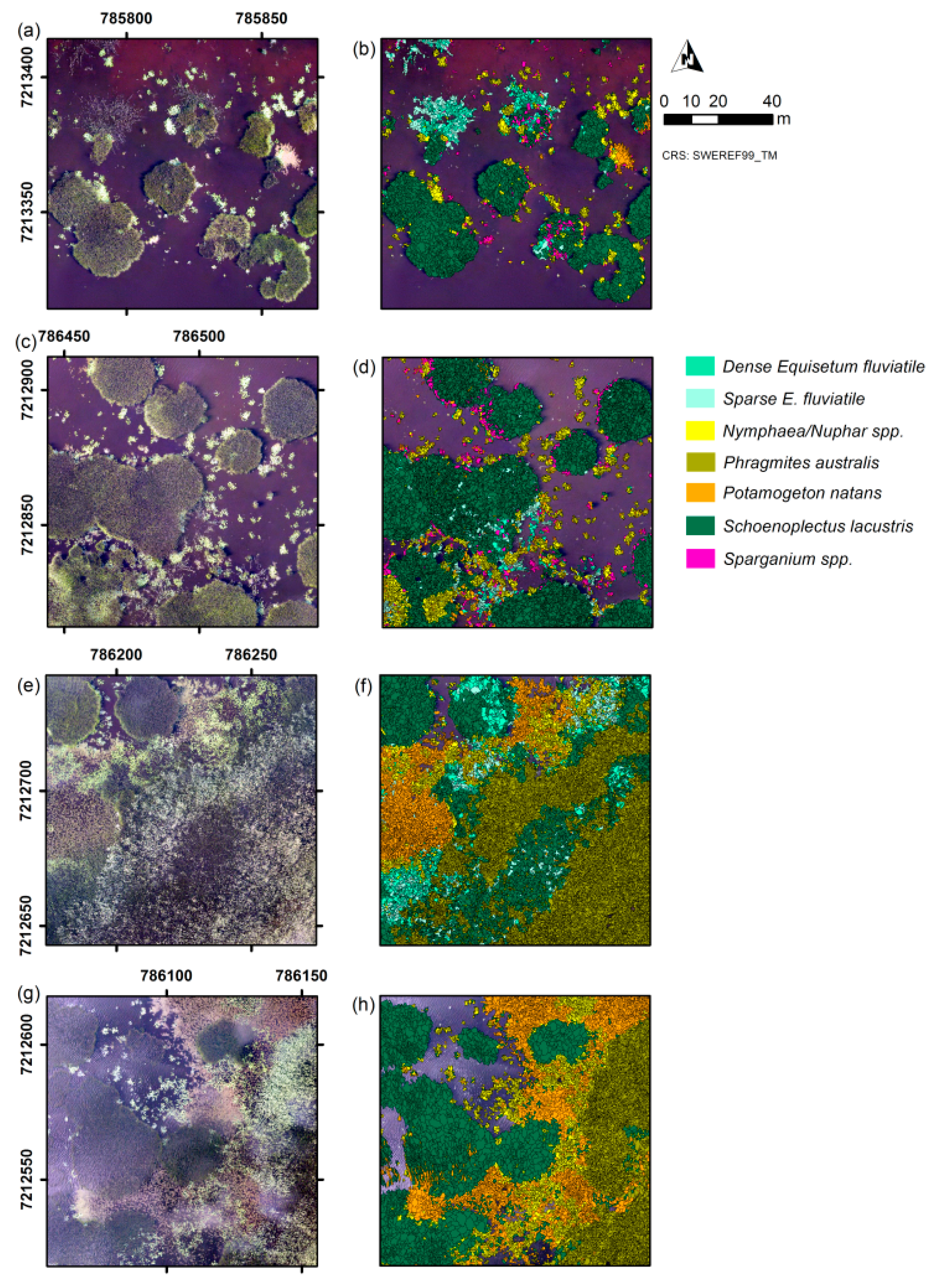
I	Schoenoplectus lacustris, Nymphaea/Nuphar spp., Equisetum fluviatile (dense), E. fluviatile (sparse), Potamogeton natans, Sparganium spp.
II	S. lacustris, Nymphaea/Nuphar spp., P. natans, Sparganium spp., E. fluviatile (sparse), E. fluviatile (dense)
III	Nymphaea/Nuphar spp., E. fluviatile (sparse), E. fluviatile (dense), P. natans, Sparganium spp.
IV	Phragmites australis, S. lacustris, P. natans, Nymphaea/Nuphar spp., E. fluviatile (dense), E. fluviatile (sparse)
V	S. lacustris, P. natans, P. australis, Nymphaea/Nuphar spp.

). More details on Ostträsket, the five test sites, and the vegetation can be found in Husson et al. [2].

2.2. Height Data

Point cloud data from which vegetation height was determined for the five test sites was derived from the original overlapping single UAS-images using the Structure-from-Motion software PhotoScan^® (Professional edition, v. 1.2.4, Agisoft LLC, St. Petersburg, Russia), because the original UAS-DSM from the orthoimage production by the external image provider was not available for this study. For each test site, the images of the respective flight block and the camera positions recorded during image acquisition were loaded into PhotoScan^®. The user-specified accuracy of the camera coordinates was set to 10 m. Blurred images were excluded from the dataset and the images were aligned (accuracy: high; pair preselection: reference; key point limit: 40,000; tie point limit: 4000). Points with low image count (≤2), high reprojection error (≥0.45), and low projection accuracy (≥40) were deleted. Camera alignment optimisation was then run in PhotoScan^® and the surface was reconstructed (building of mesh (face count: low) and texture). Ground control points with coordinates measured in the field were not available for our study. To minimize the displacement of the DSM compared to the orthoimage which was georeferenced from the beginning, 12–25 reference points per test site were selected in the orthoimage and manually placed as markers for georeferencing in PhotoScan^®. The reference points were evenly distributed throughout the whole test site with additional reference points at the corners and in the centre of the image. The user-specified accuracy of the reference points was set to 0.005 m in PhotoScan. We manually added reference points until the total XY error (average mean square error) of the reference points reached a minimum, indicating that the displacement between the DSM and the orthoimage was at a minimum. The displacement (i.e., the total XY error) at the five test sites was ≤5.6 cm. We did not have any field-based height measurements for these points. Therefore, we selected reference points at the water surface, mainly floating leaves, and assigned a value of zero as the height. Since we used the water surface as the zero height level we also subtracted 15 m from the z-values of the recorded camera positions because Lake Ostträsket is located at 15 m above sea level. When the markers were placed, a dense point cloud was produced (quality setting: high; depth filtering: mild) that was used to build a DSM (Figure 1). Due to the movement of waves and since the UAS-images were not taken simultaneously, image matching was difficult for open water surfaces and some sparse vegetation stands at Site V in regions with poor image quality. We therefore disabled interpolation for the DSM production. Initial tests showed that DSMs produced with interpolation displayed unreasonably high and/or low height values in areas with open water. By disabling interpolation, the areas with unreasonable height values could be reduced. The produced DSMs for the five test sites had a ground sampling distance of ~9 cm and a point density of ≥106 points per m². The UAS-DSMs were exported as GeoTiff-files with a pixel size of 5 cm in order to match the pixel size of the UAS-orthoimage.

2.3. Object-Based Image Analysis and Accuracy Assessment

Object-based image analysis in combination with Random Forest classification was applied to the five test sites using the software eCognition Developer^® (v. 9.1, Trimble Germany GmbH, Munich, Germany). In the current study, we performed the Random Forest classification on the growth-form and the dominant-taxon level based on spectral and textural features from the UAS-orthoimage as described in Husson et al. [2] with the only difference being that the UAS-DSM was loaded as an additional image layer in eCognition^® and a new feature for classification was added: “Mean DSM” (i.e., the mean height value for each segment). The growth-form level included three classes: Water, nymphaeid, and helophyte. For the classification at the dominant-taxon level, the water area was masked out [2]. We defined the dominant taxon as the taxon that covered the largest area in the respective vegetation stand. Seven classes were included according to the dominant taxa given in

Table 2. Overall classification accuracy (%, segment-, and area-based), Cohen’s Kappa coefficient, overall quantity disagreement (%), and overall allocation disagreement (%) for the classification based on height data combined with spectral and textural features for test sites I–V presented by the level of thematic detail (growth forms and dominant taxa). For comparison, the results from our previous study [2] based on spectral and textural features alone were reproduced in this table. Bold numbers indicate a statistically significant difference with the inclusion of height data (N = 5, α < 0.05).

Level of Thematic Detail	Growth Forms					Dominant Taxa
Site	I	II	III	IV	V	I	II	III	IV	V
Overall accuracy (segment-based)
Height, spectral, and textural features	84.6	87.1	78.9	77.7	78.0	79.1	81.1	66.4	81.9	85.4
Spectral and textural features	80.3	83.4	74.3	56.3	63.4	68.6	64.7	63.0	52.2	65.4
Difference	4.3	3.7	4.6	21.4	14.6	10.5	16.4	3.4	29.7	20.0
Overall accuracy (area-based)
Height, spectral, and textural features	94.7	92.9	82.3	76.6	74.3	82.7	85.3	63.2	82.1	86.2
Spectral and textural features	93.6	91.6	77.8	56.4	64.8	72.7	70.3	61.0	51.8	74.6
Difference	1.0	1.2	4.5	20.2	9.5	9.9	15.0	2.3	30.2	11.7
Cohen’s Kappa coefficient
Height, spectral, and textural features	0.75	0.76	0.58	0.54	0.64	0.68	0.67	0.38	0.74	0.81
Spectral and textural features	0.69	0.69	0.51	0.25	0.40	0.54	0.46	0.34	0.39	0.54
Difference	0.07	0.07	0.07	0.29	0.24	0.14	0.21	0.04	0.35	0.27
Overall quantity disagreement
Height, spectral, and textural features	6.9	6.9	11.1	18.6	11.4	10.7	10.8	20.7	13.5	6.0
Spectral and textural features	8.0	7.4	14.6	36.3	10.9	14.6	23.1	22.7	30.8	2.9
Difference	−1.1	−0.6	−3.4	−17.7	0.6	−3.9	−12.2	−2.0	−17.3	3.1
Overall allocation disagreement
Height, spectral, and textural features	8.6	6.0	10.0	3.7	10.6	10.2	8.1	12.9	4.7	8.6
Spectral and textural features	11.7	9.1	11.1	7.3	25.7	16.8	12.2	14.3	17.0	31.7
Difference	−3.1	−3.1	−1.1	−3.7	−15.1	−6.6	−4.2	−1.4	−12.4	−23.1

. To ensure full comparability between the current study and Husson et al. [2], the segments from Husson et al. [2] obtained by “Multiresolution Segmentation” based on the UAS-orthoimage alone, were used. For each test site, 40 training sample-segments per class were randomly selected from the sites’ “Reference Maps” which were manually produced with visual interpretation. More details on the production of the Reference Maps are provided in Husson et al. [2], including the classification scheme for visual interpretation with image examples for all taxa in the Supplementary Materials. At Site I, we selected only 30 training samples per dominant taxa class because there were two classes with a low total number of segments (59 and 60 segments; [2]). The training sample-segments used in both studies were identical. Also, for accuracy assessment we used exactly the same validation sample-segments as in Husson et al. ([2]; i.e., 350 randomly selected sample-segments per site). In cases where a class was represented by only a few segments, we randomly selected more samples so that there were at least ten segments for that class [2]. To evaluate the classification, a segment-based error matrix was produced. We calculated overall, Producer’s, and User’s accuracy, Cohen’s Kappa coefficient [22], as well as overall quantity disagreement and overall allocation disagreement [23]. Producer’s accuracy is the probability that a polygon belonging to a given category on the ground has also been labelled that category in the map while User’s accuracy is the probability that a polygon classified into a given category actually represents that category on the ground. The Kappa statistic takes into account the fact that even assigning labels at random results in a certain degree of accuracy. The Kappa coefficient has however been criticised as being misleading and redundant in remote sensing applications [23,24]; for this reason we have also included quantity and allocation disagreement as an alternative to Kappa [23]. Overall quantity disagreement is defined as the difference between two data sets due to an imperfect match in proportions of the mapped categories. Overall allocation disagreement is defined as the difference between two data sets due to an imperfect match between the spatial allocations of the mapped categories. Since the validation sample-segments varied in size, we also produced an area-based error matrix (related to the number of pixels inside the selected validation segments) and calculated the overall, Producer’s, and User’s accuracies to evaluate the map’s usability by assessing the correctly classified area as proposed by Radoux et al. [25].

2.4. Statistical Analysis

We used non-metric, one-sided Wilcoxon matched pairs signed-rank tests [26] at both levels of thematic detail to test for a potential increase in classification accuracy due to incorporation of height data. In other words, we compared the results from our previous study which were based on spectral and textural features from the UAS-orthoimage only [2], to our new results which were based on spectral and textural features from the UAS-orthoimage and height data from the UAS-DSM. For overall accuracy (both segment- and area-based), Kappa, overall quantity disagreement, and overall allocation disagreement, the sample size N was five and we used a significance level of α < 0.05. We also compared the Producer’s and User’s accuracies (both segment-, and area-based) with and without height data at each level of thematic detail for all classes and sites combined. Here the sample size was larger (N = 15 for growth forms and N = 27 for dominant taxa) and we used three significance levels, namely * for α < 0.025, ** for α < 0.005, and *** for α < 0.0005. For the statistical analysis we used Statistica^® software (v. 13, Dell Inc., Tulsa, OK, USA).

3. Results

The use of height data combined with spectral and textural features resulted in better classification results at all test sites, as compared to using spectral and textural features alone. The increase in overall accuracy (segment- and area-based) was statistically significant at both levels of thematic detail (T₅ = 0, p = 0.043 for all four tests).

At the growth-form level, the use of height combined with spectral and textural features gave an overall accuracy of 78%–87% (segment-based). For the five test sites, this represented an average increase of 10% (range 4%–21%, Table 2). The increase in accuracy was largest at Sites IV and V (Table 2). The correctly classified area after the inclusion of height data was 74%–95% (Table 2, area-based overall accuracy). For the five test sites, this represented an average increase of 7% (range 1%–20%, Table 2).

At the dominant-taxon level, the use of height data combined with spectral and textural features gave an overall accuracy of 66%–85% (segment-based). For the five test sites, this represented an average increase of 16% (range 3%–30%, Table 2). The correctly classified area after the inclusion of height data was 63%–86% (Table 2, area-based overall accuracy) which represented an average increase of 14% for the five test sites (range 2%–30%, Table 2). The largest increase (30%) in overall accuracy (segment- and area-based) was observed at Site IV (Table 2, Figure 2e,f), which was the site with the most complex vegetation and that showed the lowest overall classification accuracy in the study without height data [2]. In comparison to the other test sites, the increase at Site III was small (3% in the segment-based and 2% in the area-based assessment; Table 2). The orthoimages and produced vegetation maps for dominant taxa at Sites I, II, IV, and V are included in Figure 2.

Kappa increased for all test sites when the height data were added (Table 2). At both levels of thematic detail the increase of Kappa was statistically significant (T₅ = 0, p = 0.043 for both tests). Overall quantity disagreement increased slightly at Site V (Table 2), but decreased at all other sites (Table 2), however, the difference was not statistically significant (growth-form level: T₅ = 1.5, p = 0.110; dominant-taxon level: T₅ = 2.0, p = 0.140). Overall allocation disagreement decreased significantly at all test sites and levels of thematic detail (Table 2; T₅ = 0, p = 0.043 for both levels of thematic detail). At both levels of thematic detail, the overall quantity disagreement was larger than the overall allocation disagreement at the majority of sites. Complete error matrices for both levels of thematic detail at all test sites and differences between error matrices from the classifications with and without height data are included in the Supplementary Material (Table S1).

Producer’s and User’s accuracies at the growth-form level increased by including height data for the majority of classes and sites (

Table 3. Producer’s and User’s accuracy (%, segment-, and area-based), number of validation segments, and total area of validation segments (m²) for the classification of growth-forms based on height data combined with spectral and textural features presented by test site and class: water (W), nymphaeid (N), and helophyte (H). For comparison, the results from our previous study [2] based on spectral and textural features alone were reproduced in this table. Bold numbers indicate a statistically significant increase when height data were included and stars indicate the level of significance (* for α < 0.025, ** for α < 0.005, and *** for α < 0.0005). Valid N is the total number of differences with either a positive or negative sign.

	Site I			Site II			Site III			Site IV			Site V			Wilcoxon Signed-Rank Test
	W	N	H	W	N	H	W	N	H	W	N	H	W	N	H	Valid N	T	p
Producer’s accuracy (segment-based)
Height, spectral, and textural features	83	88	84	89	68	95	65	83	75	90	90	74	93	88	65	12	0	0.002 **
Spectral and textural features	81	82	79	89	59	92	63	78	69	90	82	49	93	68	53
User’s accuracy (segment-based)
Height, spectral, and textural features	98	65	88	86	94	86	83	93	43	25	58	98	38	88	87	14	11	0.009 *
Spectral and textural features	97	58	84	89	84	82	85	92	35	25	33	92	39	74	63
No. of validation segments	106	68	176	57	87	206	52	246	52	10	71	274	28	163	159
Producer’s accuracy (area-based)
Height, spectral, and textural features	97	87	89	96	63	96	90	74	80	92	89	73	96	86	62	12	0	0.002 **
Spectral and textural features	97	83	87	96	54	96	89	70	68	92	77	49	96	69	56
User’s accuracy (area-based)
Height, spectral, and textural features	99	64	91	96	94	90	90	93	58	35	57	98	32	93	88	15	8	0.003 **
Spectral and textural features	99	59	89	97	89	88	87	92	49	35	30	92	34	80	73
Total area of validation segments	458	37	177	162	39	176	145	121	66	18	42	201	30	120	168

), and the overall increases of segment- and area-based Producer’s and User’s accuracies were statistically significant (T and p values given in Table 3). The largest increases were observed for the classes of nymphaeid and helophyte at Sites IV and V (Table 3). For water, Producer’s and User’s accuracies were only marginally affected by the inclusion of height data (Table 3).

Producer’s and User’s accuracies at the dominant-taxon level varied between classes and sites (

Table 4. Producer’s and User’s accuracy (%, segment-, and area-based), number of validation segments, and total area of validation segments (m²) for the classification of dominant taxa based on height data combined with spectral and textural features for Sites I–V presented by vegetation class. For comparison, the results from our previous study [2] based on spectral and textural features alone were reproduced in this table. Vegetation classes have been abbreviated as follows: Equisetum fluviatile (E.f.), Nymphaea/Nuphar spp. (N./N. spp.), Phragmites australis (P.a.), Potamogeton natans (P.n.), Schoenoplectus lacustris (S.l.), and Sparganium spp. (S. spp.). Bold and italic numbers indicate an increase of ≥5% when height data were included.

	Vegetation Class
	Sparse E.f.	Dense E.f.	N./N. spp.	P.a.	P.n.	S.l.	S. spp.
Site I
Producer’s accuracy (segment-based)
Height, spectral, and textural features	60	56	83		80	83	50
Spectral and textural features	60	48	79		80	68	40
User’s accuracy (segment-based)
Height, spectral, and textural features	45	44	93		53	97	16
Spectral and textural features	41	33	78		47	92	11
No. of validation segments	15	27	95		10	206	10
Producer’s accuracy (area-based)
Height, spectral, and textural features	76	43	86		91	87	48
Spectral and textural features	76	41	83		91	74	31
User’s accuracy (area-based)
Height, spectral, and textural features	38	49	91		72	98	13
Spectral and textural features	33	33	71		66	95	8
Total area of validation segments	12	24	50		10	214	5
Site II
Producer’s accuracy (segment-based)
Height, spectral, and textural features	50	80	71		20	90	70
Spectral and textural features	50	70	70		20	65	70
User’s accuracy (segment-based)
Height, spectral, and textural features	21	47	93		11	97	35
Spectral and textural features	12	29	84		6	92	27
No. of validation segments	10	10	90		10	230	10
Producer’s accuracy (area-based)
Height, spectral, and textural features	63	61	73		13	91	72
Spectral and textural features	63	59	71		13	72	72
User’s accuracy (area-based)
Height, spectral, and textural features	26	44	89		5	99	33
Spectral and textural features	15	18	81		3	96	23
Total area of validation segments	7	4	40		4	205	5
Site III
Producer’s accuracy (segment-based)
Height, spectral, and textural features	50	59	70		50		70
Spectral and textural features	48	59	66		50		70
User’s accuracy (segment-based)
Height, spectral, and textural features	54	28	95		13		30
Spectral and textural features	44	24	94		13		32
No. of validation segments	40	22	273		12		10
Producer’s accuracy (area-based)
Height, spectral, and textural features	64	71	61		72		67
Spectral and textural features	62	71	57		72		67
User’s accuracy (area-based)
Height, spectral, and textural features	80	37	95		18		36
Spectral and textural features	75	32	95		20		38
Total area of validation segments	61	22	131		11		7
Site IV
Producer’s accuracy (segment-based)
Height, spectral, and textural features	90	20	66	100	94	59
Spectral and textural features	80	40	61	48	88	43
User’s accuracy (segment-based)
Height, spectral, and textural features	30	10	87	93	79	97
Spectral and textural features	17	9	68	81	38	69
No. of validation segments	10	10	41	170	33	100
Producer’s accuracy (area-based)
Height, spectral, and textural features	98	13	59	100	96	74
Spectral and textural features	92	23	56	43	89	51
User’s accuracy (area-based)
Height, spectral, and textural features	32	12	82	95	82	96
Spectral and textural features	19	11	70	83	34	77
Total area of validation segments	9	12	22	95	22	97
Site V
Producer’s accuracy (segment-based)
Height, spectral, and textural features			95	100	76	74
Spectral and textural features			55	53	78	73
User’s accuracy (segment-based)
Height, spectral, and textural features			83	89	85	84
Spectral and textural features			49	53	79	80
No. of validation segments			78	85	96	91
Producer’s accuracy (area-based)
Height, spectral, and textural features			93	100	77	85
Spectral and textural features			49	62	79	84
User’s accuracy (area-based)
Height, spectral, and textural features			82	83	87	89
Spectral and textural features			53	57	77	87
Total area of validation segments			41	51	89	134

). For the majority of classes and sites, Producer’s and User’s accuracies increased when height data were included (Table 4), and the overall increases of segment- and area-based Producer’s and User’s accuracies were statistically significant (T and p values given in

Table 5. Valid N-, T-, and p-values from one-sided Wilcoxon matched pairs signed-rank tests for Producer’s and User’s accuracy (segment- and area-based) at the dominant taxon level for all classes and sites combined. Bold numbers indicate a statistically significant increase when height data were included and stars indicate the level of significance (* for α < 0.025, ** for α < 0.005, and *** for α < 0.0005). Valid N is the total number of differences with either a positive or negative sign.

	Valid N	T	p
Producer’s accuracy (segment-based)	19	18	0.00194 **
User’s accuracy (segment-based)	27	5	0.00001 ***
Producer’s accuracy (area-based)	20	20	0.00151 **
User’s accuracy (area-based)	27	8	0.00001 ***

). The class of P. australis (emergent, present at Sites IV and V) showed the largest increase of Producer’s accuracy (Table 4). At Site IV, the reduced confusion of all taxa with P. australis resulted in increased User’s accuracies (≥12%) for all classes except for dense E. fluviatile which increased by only 1% (Table 4 and Table S1). Also at Site IV, the confusion between floating-leaved P. natans and emergent S. lacustris was reduced (Table S1). At Site V, mainly the confusion between floating-leaved Nymphaea/Nuphar spp. and emergent P. australis was reduced (Table S1). At Sites I and II, the confusion of emergent S. lacustris with all other taxa was reduced (Table S1). In the study based on spectral and textural features alone, the two E. fluviatile classes, P. natans and Sparganium spp., in all cases had a lower User’s accuracy than Producer’s accuracy, indicating a large number of false inclusions [2]. The inclusion of height data reduced most differences between the User’s and Producer’s accuracies, but User’s accuracies were still lower than Producer’s accuracies in all cases except for sparse E. fluviatile at Site III (Table 4). For the two classes that were most reliably classified without height data, Nymphaea/Nuphar spp. and S. lacustris, the inclusion of height data further increased both Producer’s and User’s accuracies at all sites (generally between 0.3% and 44%; Table 4).

4. Discussion

When height data from a UAS-DSM were included in the classification along with spectral and textural features from a UAS-orthoimage, the classification accuracy was higher than when spectral and textural features alone were used. The inclusion of height data successfully reduced the confusion between taxa that belonged to different growth forms (emergent and floating-leaved). In contrast to the study based on spectral and textural features alone [2], where emergent P. australis was confused with all other taxa, it now belonged to the most reliably classified taxa. P. australis was the tallest taxa in our classification [3]. It has a bright green colour (similar to Nymphaea/Nuphar spp., Sparganium spp., and sun exposed S. lacustris) which is easy to detect against a darker background of, for example, dark green vegetation or water.

In the previous study [2], the classification of S. lacustris was also problematic due to the high variation in spectral appearance within this taxon. Typically, at the edge of stands of S. lacustris, stems are bent and more exposed to the sun than those in the interior of the stands. This results in the former looking more brightly green than the majority of S. lacustris stems. In addition, we observed areas with low cover within S. lacustris stands, where stems were probably straighter than the majority of S. lacustris stems; these areas appeared darker. Therefore, in the classification based on spectral and textural features alone, S. lacustris was often confused with other taxa which decreased the User’s accuracy, especially of taxa that covered smaller total areas than the relatively common S. lacustris. With the inclusion of height data, the classification of S. lacustris was more reliable.

Compared to the other two emergent taxa, E. fluviatile was the least affected by the inclusion of height data. E. fluviatile had the lowest vegetation height among the emergent taxa in this study [3]. The two E. fluviatile classes were mainly confused with each other and S. lacustris (also emergent) but, especially at Site III it was also confused with Nymphaea/Nuphar spp. (floating-leaved). The inclusion of height data could not substantially reduce the confusion between these classes even though they belong to different growth forms. E. fluviatile has a straight, needle-like shape, and the fine leaves are also needle-like and were almost invisible on the UAS-images. At Site III, E. fluviatile rarely formed stands that were dense enough to completely obscure the water surface and formed to a large extent mixed vegetation stands with Nymphaea/Nuphar spp. This probably led to a larger variation in mean height values for E. fluviatile-covered segments at this site. In our previous study, we found that Site III had the highest proportion of misclassifications where a non-dominant taxon was wrongly classified as the dominant taxon. E. fluviatile was the only emergent taxa present at Site III, which explains the relatively small increase in classification accuracy at this test site.

The addition of height data also helped to reduce the confusion among emergent taxa, for example, between P. australis and S. lacustris (Sites IV and V), between P. australis and E. fluviatile (Site IV), and between S. lacustris and E. fluviatile (Sites I, II, and IV). This indicates that the UAS-DSM successfully resolved even smaller differences in vegetation height than between emergent and floating-leaved taxa.

The reduced confusion among growth forms and taxa resulted in very good classification accuracies (at least ~80%) at most test sites, both at the growth-form and the dominant-taxon level, including the site with the largest vegetation complexity. At Site V, the test site with low image quality, the overall classification accuracy increased, indicating that the inclusion of height data further increased the robustness of the classification process. These results show good potential for operative mapping and monitoring of aquatic vegetation at a high level of thematic detail and in an automated way, which is important to time-efficiently cover larger areas.

Conventional orthoimage production is often based on less dense point clouds from which objects with heights above ground level such as vegetation or buildings are removed. Our suggested method requires the production of true orthoimages with unfiltered dense point clouds (ca. >100 points per m²). This implies increased operator time and computational costs compared to conventional orthoimages. Thanks to recent developments in digital photogrammetry and computer vision, an increasing number of user-friendly software programmes for UAS-image processing are available. The calculation of 3D point clouds from overlapping UAS-images is usually integrated in the workflow of these programmes and is typically part of the production of a true UAS-orthoimage with high spatial accuracy. The height information from image-based dense point clouds generated with Structure-from-Motion software based on algorithms such as Semi-Global Matching [27] can be comparable to that from airborne LiDAR [28] and even low-cost systems such as a UAS equipped with a consumer grade camera allow for surface reconstructions of high quality when the image overlap is high [29]. Once a dense point cloud is constructed, the production of a UAS-DSM is only a minor effort. Regarding the high increase in accuracy achieved in our study, UAS-DSMs have a large potential to efficiently improve the classification results when combined with spectral data.

For our study, UAS-DSMs for the test sites were produced after the original UAS-orthoimage production and independent from the orthoimage. This was done because the original UAS-orthoimage was produced by an external image processing company and the point cloud was not initially made available for our study. The independent production of the UAS-orthoimage and UAS-DSMs resulted in a spatial displacement between the two, which is a potential source of error in our classification. The spatial displacement varied from site to site but had an average of 4.5 cm, and a maximum of 5.6 cm, which is about the size of one pixel (5 cm). For future studies, we recommend producing the UAS-DSM together with the UAS-orthoimage to avoid differences in data co-registration.

Ground control points with height measurements were missing in our study. This was solved by using the water surface as the zero level. In our study, the internal relative differences in vegetation height were most important since our focus was on the classification of different growth-forms with relatively large differences in vegetation height. The maximum vegetation heights in the UAS-DSMs of the five test sites are plausible. However, when the UAS-DSM is to be used for the extraction of absolute height values, for example, for biomass estimation, height measurements of reference points in the field are recommended for calibration.

5. Conclusions

At five test sites with varying vegetation complexity and image quality at a lake in northern Sweden, the inclusion of height data in addition to spectral and textural features from a true-colour UAS-orthoimage with 5-cm pixels significantly increased the classification accuracy of non-submerged aquatic vegetation as compared to using spectral and textural features alone. The inclusion of height data reduced the confusion between taxa that appeared similar in the image but belonged to different growth forms (emergent and floating-leaved), as well as among emergent taxa. The overall classification accuracy increased to at least ~80% at all five test sites for growth forms and at four out of five test sites for dominant taxa. The combination of true-colour UAS-orthoimages with height data derived from dense 3D point clouds from image matching has a large potential to efficiently increase the accuracy of automated classification. This approach improves the possibilities for operative mapping and monitoring of non-submerged aquatic vegetation at a high level of thematic detail covering larger areas such as entire lakes.

References

- Anderson, K.; Gaston, K.J. Lightweight unmanned aerial vehicles will revolutionize spatial ecology. Front. Ecol. Environ. 2013, 11, 138–146. [Google Scholar] [CrossRef]
- Husson, E.; Ecke, F.; Reese, H. Comparison of manual mapping and automated object-based image analysis of non-submerged aquatic vegetation from very-high-resolution UAS images. Remote Sens. 2016, 8, 724. [Google Scholar] [CrossRef]
- Mossberg, B.; Stenberg, L. Den Nya Nordiska Floran; Wahlström & Widstrand: Aurskog, Norge, 2006. [Google Scholar]
- Tempfli, K.; Kerle, N.; Huurneman, G.C.; Janssen, L.L.E. Principles of Remote Sensing; ITC: Enschede, The Netherlands, 2009. [Google Scholar]
- Colwell, R. Manual of Photographic Interpretation; American Society of Photogrammetry: Washington, DC, USA, 1960. [Google Scholar]
- Madden, M.; Jordan, T.; Bernardes, S.; Cotten, D.L.; O’Hare, N.; Pasqua, A. Unmanned aerial systems and structure from motion revolutionize wetlands mapping. In Wetlands: Applications and Advances; Tiner, R.W., Lang, M.W., Klemas, V.V., Eds.; CRC Press: Boca Raton, FL, USA, 2015; pp. 195–219. [Google Scholar]
- Colomina, I.; Molina, P. Unmanned aerial systems for photogrammetry and remote sensing: A review. ISPRS J. Photogramm. Remote Sens. 2014, 92, 79–97. [Google Scholar] [CrossRef]
- Cunliffe, A.M.; Brazier, R.E.; Anderson, K. Ultra-fine grain landscape-scale quantification of dryland vegetation structure with drone-acquired structure-from-motion photogrammetry. Remote Sens. Environ. 2016, 183, 129–143. [Google Scholar] [CrossRef] [Green Version]
- Ke, Y.H.; Quackenbush, L.J.; Im, J. Synergistic use of Quickbird multispectral imagery and Lidar data for object-based forest species classification. Remote Sens. Environ. 2010, 114, 1141–1154. [Google Scholar] [CrossRef]
- Nordkvist, K.; Granholm, A.-H.; Holmgren, J.; Olsson, H.; Nilsson, M. Combining optical satellite data and airborne laser scanner data for vegetation classification. Remote Sens. Lett. 2012, 3, 393–401. [Google Scholar] [CrossRef]
- Granholm, A.H.; Olsson, H.; Nilsson, M.; Allard, A.; Holmgren, J. The potential of digital surface models based on aerial images for automated vegetation mapping. Int. J. Remote Sens. 2015, 36, 1855–1870. [Google Scholar] [CrossRef]
- Reese, H.; Nordkvist, K.; Nyström, M.; Bohlin, J.; Olsson, H. Combining point clouds from image matching with Spot 5 multispectral data for mountain vegetation classification. Int. J. Remote Sens. 2015, 36, 403–416. [Google Scholar] [CrossRef]
- Reese, H.; Nyström, M.; Nordkvist, K.; Olsson, H. Combining airborne laser scanning data and optical satellite data for classification of alpine vegetation. Int. J. Appl. Earth Obs. Geoinf. 2014, 27, 81–90. [Google Scholar] [CrossRef]
- Gillan, J.K.; Karl, J.W.; Duniway, M.; Elaksher, A. Modeling vegetation heights from high resolution stereo aerial photography: An application for broad-scale rangeland monitoring. J. Environ. Manag. 2014, 144, 226–235. [Google Scholar] [CrossRef] [PubMed]
- Rampi, L.P.; Knight, J.F.; Pelletier, K.C. Wetland mapping in the upper midwest United States: An object-based approach integrating Lidar and imagery data. Photogramm. Eng. Remote Sens. 2014, 80, 439–448. [Google Scholar] [CrossRef]
- Al-Rawabdeh, A.; He, F.N.; Moussa, A.; El-Sheimy, N.; Habib, A. Using an unmanned aerial vehicle-based digital imaging system to derive a 3D point cloud for landslide scarp recognition. Remote Sens. 2016, 8, 95. [Google Scholar] [CrossRef]
- Vetrivel, A.; Gerke, M.; Kerle, N.; Vosselman, G. Segmentation of UAV-based images incorporating 3D point cloud information. In Proceedings of the Joint ISPRS Conference on Photogrammetric Image Analysis (PIA) and High Resolution Earth Imaging for Geospatial Information (HRIGI), Munich, Germany, 25–27 March 2015.
- Lechner, A.M.; Fletcher, A.; Johansen, K.; Erskine, P. Characterising upland swamps using object-based classification methods and hyper-spatial resolution imagery derived from an umanned aerial vehicle. In Proceedings of the XXII ISPRS Congress, Melbourne, Australia, 25 August–1 September 2012.
- Kuria, D.N.; Menz, G.; Misana, S.; Mwita, E.; Thamm, H.; Alvarez, M.; Mogha, N.; Becker, M.; Oyieke, H. Seasonal vegetation changes in the Malinda wetland using bi-temporal, multi-sensor, very high resolution remote sensing data sets. Adv. Remote Sens. 2014, 3, 33–48. [Google Scholar] [CrossRef]
- Tamminga, A.; Hugenholtz, C.; Eaton, B.; Lapointe, M. Hyperspatial remote sensing of channel reach morphology and hydraulic fish habitat using an unmanned aerial vehicle (UAV): A first assessment in the context of river research and management. River Res. Appl. 2015, 31, 379–391. [Google Scholar] [CrossRef]
- Boon, M.A.; Greenfield, R.; Tesfamichael, S. Wetland assessment using unmanned aerial vehicle (UAV) photogrammetry. In Proceedings of the XXIII ISPRS Congress, Prague, Czech Republic, 12–19 July 2016.
- Congalton, R.G. A review of assessing the accuracy of classifications of remotely sensed data. Remote Sens. Environ. 1991, 37, 35–46. [Google Scholar] [CrossRef]
- Pontius, R.G.; Millones, M. Death to kappa: Birth of quantity disagreement and allocation disagreement for accuracy assessment. Int. J. Remote Sens. 2011, 32, 4407–4429. [Google Scholar] [CrossRef]
- Olofsson, P.; Foody, G.M.; Herold, M.; Stehman, S.V.; Woodcock, C.E.; Wulder, M.A. Good practices for estimating area and assessing accuracy of land change. Remote Sens. Environ. 2014, 148, 42–57. [Google Scholar] [CrossRef]
- Radoux, J.; Bogaert, P.; Fasbender, D.; Defourny, P. Thematic accuracy assessment of geographic object-based image classification. Int. J. Geogr. Inf. Sci. 2011, 25, 895–911. [Google Scholar] [CrossRef]
- Zar, J.H. Biostatistical Analysis; Prentice-Hall Inc.: Upper Saddle River, NJ, USA, 1999. [Google Scholar]
- Hirschmüller, H. Stereo processing by semi-global matching and mutual information. IEEE Trans. Pattern Anal. Mach. Intell. 2008, 30, 328–341. [Google Scholar] [CrossRef] [PubMed]
- Leberl, F.; Irschara, A.; Pock, T.; Meixner, P.; Gruber, M.; Scholz, S.; Wiechert, A. Point clouds: Lidar versus 3D vision. Photogramm. Eng. Remote Sens. 2010, 76, 1123–1134. [Google Scholar] [CrossRef]
- Haala, N.; Cramer, M.; Rothermel, M. Quality of 3D point clouds from highly overlapping UAV imagery. In Proceedings of the Conference on Unmanned Aerial Vehicles in Geomatics (UAV-g), Rostock, Germany, 4–6 September 2013.