Estimating Snow Mass and Peak River Flows for the Mackenzie River Basin Using GRACE Satellite Observations

Abstract

Flooding is projected to increase with climate change in many parts of the world. Floods in cold regions are commonly a result of snowmelt during the spring break-up. The peak river flow (Q_peak) for the Mackenzie River, located in northwest Canada, is modelled using the Gravity Recovery and Climate Experiment (GRACE) satellite observations. Compared with the observed Q_peak at a downstream hydrometric station, the model results have a correlation coefficient of 0.83 (p < 0.001) and a mean absolute error of 6.5% of the mean observed value of 28,400 m³·s⁻¹ for the 12 study years (2003–2014). The results are compared with those for other basins to examine the difference in the major factors controlling the Q_peak. It was found that the temperature variations in the snowmelt season are the principal driver for the Q_peak in the Mackenzie River. In contrast, the variations in snow accumulation play a more important role in the Q_peak for warmer southern basins in Canada. The study provides a GRACE-based approach for basin-scale snow mass estimation, which is largely independent of in situ observations and eliminates the limitations and uncertainties with traditional snow measurements. Snow mass estimated from the GRACE data was about 20% higher than that from the Global Land Data Assimilation System (GLDAS) datasets. The model is relatively simple and only needs GRACE and temperature data for flood forecasting. It can be readily applied to other cold region basins, and could be particularly useful for regions with minimal data.

1. Introduction

Forecasting peak river flow is of great interest to flood control and emergency service agencies, hydropower plant operators, and anyone interested in regulating river flows and flood plain ecosystem assessment. Flooding is one of the most damaging natural disasters in the world. It results in human hardship, negative effects on human activities, and billions of dollars of economic loss per year [1,2]. On the other hand, the magnitudes of peak river flows or floods are critical to a healthy environment. Floods can benefit the natural environment and sustain many ecosystems. For instance, the recurrent inundation of the Peace-Athabasca Delta in the Mackenzie River Basin (MRB) in Canada has fostered an environment in which plant and animal life has achieved a balance dependent on flooding. In fact, water spilling across the floodplain nourishes the wetlands of many major deltas in Canada [3]. Floods are projected to increase with a warming climate in the future [4]. Thus, it is of considerable value to apply new technologies to improve forecasts regarding the timing and magnitude of peak river flows.

Peak river flow in cold regions is commonly a result of snowmelt during the spring break-up, or the subarctic nival regime [5]. During winter most of the precipitation is in the form of snow, which accumulates in the basins until the spring breakup. As the spring freshet season approaches, the importance of temperature variations increases. A late gradual spring warming may release the water from the snowpack slowly, producing a small peak. By contrast, a rapid increase in the air temperature above 0 °C may lead to a rapid snowmelt, resulting in huge quantities of water released from the snowpack. Meltwater is unable to infiltrate frozen ground and runs off over the ground surface to rivers and lakes, resulting in large peak flows or floods. As such, major factors determining the magnitude of river peaks or floods during the freshet usually include the amount of snow water equivalent (SWE) accumulated during the winter season and the temporal patterns of air temperature variations in the snowmelt season.

Snowmelt runoff floods are the most common type of flooding in Canada [3,6,7,8]. Forecasting peak flows or floods for rivers in cold regions, regardless of the methods being used, heavily relies on information for SWE and air temperature. Basin-scale SWE can be estimated by the difference of snowfall and water loss from snow sublimation and blowing snow over the basin. Unfortunately, accurately estimating snowfall, even at the site level, is difficult and often has large uncertainties. For example, previous studies show that the snow gauge measurement errors at climate stations can be as high as 50% due to the wind-induced under-catch and the difficulties in recording the many trace events [9]. Snow sublimation and blowing snow estimations are even more difficult and often have large uncertainties due to the poor understanding of the cold region processes and lack of reliable data [10,11]. In addition, cold regions commonly have very sparse observational networks. For instance, the density of climate stations in the Canadian Northwest Territory is only about two stations per 100,000 km² [12]. This sparse density of stations, together with the possible limitations in the spatial representativeness of the stations, makes the up-scaling of SWE from site to basin-scale extremely unreliable.

Remote sensing satellites using optical or microwave sensors can be used to map the spatial distribution of snow cover and to address the weakness of regional representativeness of the site measurements (e.g., [13,14]). For the estimation of SWE, these remote sensing approaches rely on indirect estimates for retrieving snow parameters such as snow cover area, snowpack depth, density, liquid and ice content, etc. The retrieval of these snow parameters from satellite data can be significantly affected by the conditions of climate (such as the temperature effect on snow density), atmosphere (such as cloud contamination impact on optical imagery), land surface (such as vegetation cover and topography impacts), and snowpack thickness [15]. Moreover, the SWE models from remote sensing approaches heavily depend on in situ data for calibration and validation, which will propagate the errors in the in situ measurements to the remote sensing SWE products [16]. Due to the difficulties mentioned above, spatial snow products from traditional in situ or remote sensing approaches often have large uncertainties. Recent studies have found that errors in snow data are the principal contribution to the water budget imbalance in cold-region basins [17,18,19]. Consequently, accurate estimation of basin-scale SWE is a key challenge in improving flood forecasting over cold region rivers.

The Gravity Recovery and Climate Experiment (GRACE) satellite mission provides a new tool for monitoring variations in the terrestrial total water storage (TWS) based on measured temporal variations of the Earth’s gravity field [20]. GRACE-based estimates of terrestrial TWS include the variations of groundwater, soil moisture, surface water, snow, and ice. TWS data from GRACE have been successfully used in hydrological studies including characterizing basin storage-river discharge relationships (e.g., [21]) and glacier and ice cap changes (e.g., [22]). A variety of methods are used to separate SWE from other TWS components [23,24,25]. A big advantage of GRACE over other remote sensing SWE retrieval methods is that it neither requires the data for snowfall and snow loss nor the site-to-basin upscaling process. It also eliminates most of the limitations imposed by the climate, atmosphere, land surface, and snowpack thickness conditions as mentioned above. Comparisons of GRACE-based SWE with model results and microwave observations [23,25,26] have demonstrated a high degree of confidence in the ability of correctly retrieving SWE from the GRACE TWS. 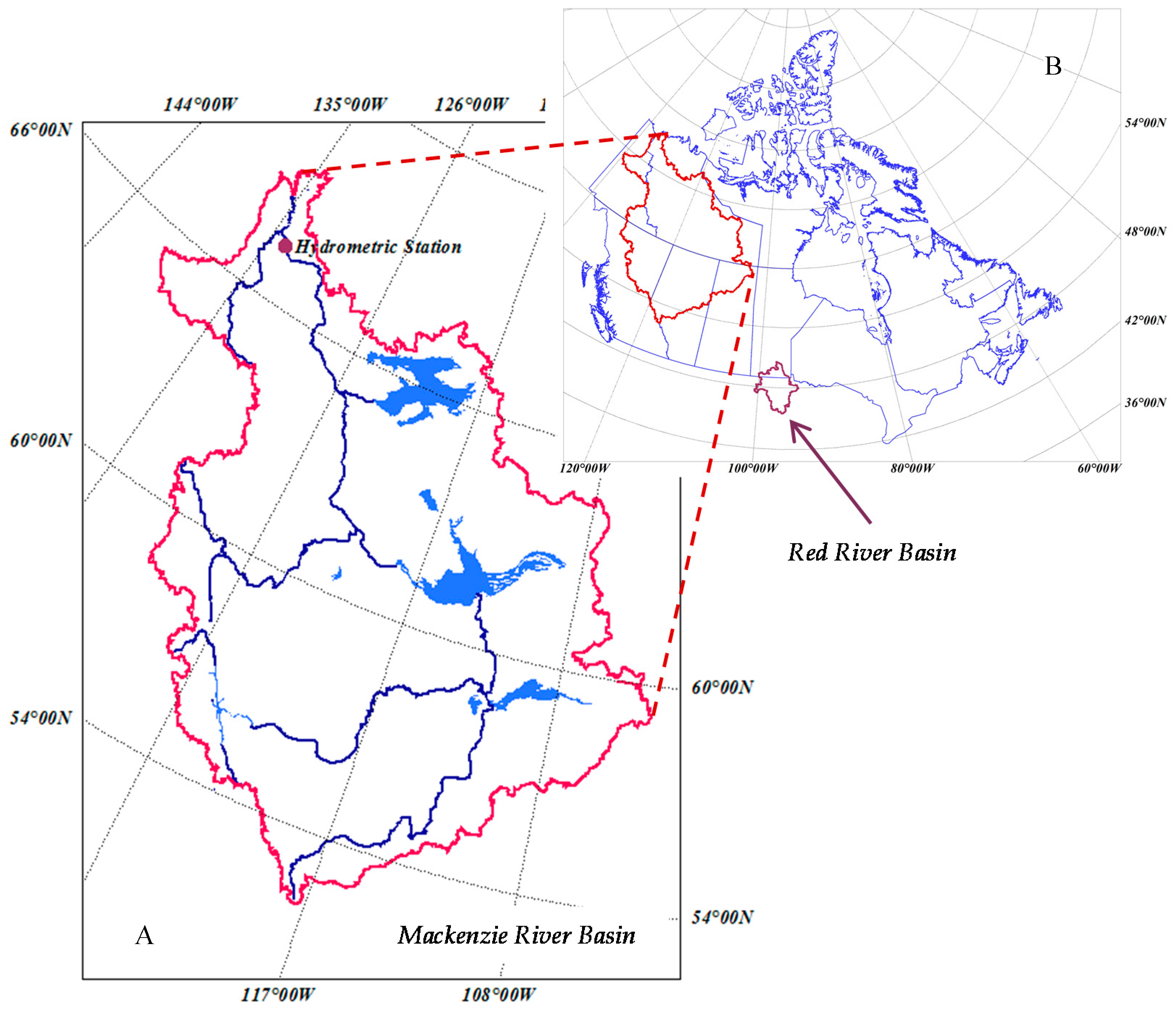In a recent study, Wang and Russell [27] developed a mass balance-based method for estimating SWE from GRACE TWS and, for the first time, applied it in developing a flood forecasting model. The model was applied to the Red River Basin (RRB), a USA-Canada transboundary basin located in central North America (Figure 1). Peak river flows estimated by the model were found to compare very well with the observed values.

The GRACE data has a relatively coarse resolution of about ~330 km (108,900 km²) at degree 60. The RRB has a drainage area of 116,500 km², which is at the nominal resolution scale of the GRACE satellites. The size limitation was found to contribute significantly to the data uncertainties in the GRACE TWS for the basin, which substantially impacted the accuracy in the peak flow estimates [27]. Nevertheless, it was found that the SWE accumulation during the snow season is the major driver determining the peak flow magnitude for the RRB, with temperature variations playing the secondary role. Whether this conclusion applies to, and what the major drivers in other basins are, still remain to be identified.

The objectives of this study are: (1) to evaluate and assess the performance of the Wang and Russell model [27] in estimating the peak river flows for the Mackenzie River Basin (MRB, Figure 1). The MRB has a large drainage area of 1.8 × 10⁶ km². This largely eliminates the constraints imposed by the coarse resolution of GRACE data; (2) to investigate differences in the major drivers controlling the peak flows for the two basins (MRB and RRB). The results were also compared to that for the Lower Fraser River (LFR) obtained in a separate study to help better understand the roles of environmental factors in determining flood and their variations with different hydroclimatic conditions; (3) to provide a mass balance-based approach for SWE estimates using GRACE data. It is worth noting that the MRB is among the most extensively studied basins in the world [28] due to its significance in local and global climate and hydrology. Several recent studies have quantified the temporal flow patterns and the water budget for the MRB as well as its sub-basins using GRACE observations [18,29,30]. The focus of this study is not the physically-based process modelling, but the use of GRACE observations to examine Mackenzie basin scale performance of peak river flows. A general goal of this study is to demonstrate a relatively simple method that only needs GRACE and temperature data input for peak river flow or flood forecasting. The model can be particularly useful for regions with spare observation networks, and can be used in combination with other available methods to help improve the accuracy in river flood forecasting over cold regions.

2. Methods

2.1. Model Description

The model simulates the magnitude of peak river flows for basin scale discharge by calculating two components of peak surface runoff from snowmelt and baseflow. The major calculations include: estimating the snow season baseflow using a modified linear reservoir model, estimating snow mass or SWE at the time of spring break up using GRACE observations, estimating daily peak snowmelt rate using a temperature index model, and determining the magnitudes of peak river flows as the sum of estimated peak surface runoff and baseflow (Figure 2). The major modelling steps are described below.

Step 1: Determining snow season

This study is only concerned with the snow season, defined as the time period from the start (t₀) of snow accumulation in late autumn to the snow breakup (t_b) the next spring (Figure 3). The t₀ is determined by the criteria of (1) the first precipitation event in late fall when the daily average temperature T_a is below 0 °C and (2) the accumulated T_a after this date remains negative. The first criterion is applied to ensure that the precipitation is in the form of snow. The second criterion is to exclude temporary snowfalls that are likely to melt away in early winter. After the date of t₀, the net snow mass from snowfall, snow sublimation, blowing snow, etc., accumulates over the basin in the winter season during which the T_a remains far below 0 °C as shown in Section 3.1. The spring breakup time t_b is determined when (1) the daily average temperature T_a rises above 0 °C and (2) the accumulated T_a after this date remains above zero. These criteria are applied to ensure that the heat conditions of the basin will lead to the spring breakup, while possible minor snowmelt events in the snow season, in case the T_a momentarily rises above 0 °C, are excluded.

Step 2: Determining total water storage change at time t₀ and t_b

The total basin water storage at t₀, i.e., TWS₀, is estimated by linearly interpolating the GRACE TWS for the two months before and after t₀. Similarly, the basin total water storage at t_b, i.e., TWS_b, is estimated by linearly interpolating the GRACE TWS for the two months before and after t_b. The simple interpolation treatment reflects the limitations of the monthly temporal resolution of GRACE data on our snowmelt modelling scheme which is at the daily time step. Fortunately, the variations of TWS around t₀ and t_b are small as can be seen in Figure 4c, which largely reduce the uncertainties in the TWS₀ and TWS_b estimates. Indeed, we tested the modelling approaches by determining TWS₀ using the minimum TWS for the two months before and after t₀, and determining TWS_b using the maximum TWS for the two months before and after t_b. We found the impacts on the modelling results are small. This will be discussed more in the Discussion Section. The TWS₀ represents the maximum amount of non-snow water in the basin during the snow season. It mainly consists of the surface water (e.g., in rivers and lakes), soil water, and groundwater, part of which will be discharged out of the basin in the snow season. The TWS_b represents the sum of snow mass accumulated during the snow season (S_b) and the non-snow water left in the basin at time t_b (W_n-s). Obviously, the W_n-s is the TWS₀ minus the total basin discharge during the snow season Q_sum (Figure 3). As such, to determine the snow mass at the spring breakup S_b, it is required to estimate Q_sum.

Step 3: Modelling baseflow rate Q_base and snow season total discharge Q_sum

Besides the requirement of Q_sum for estimating S_b as mentioned above, the baseflow rate Q_base also needs to be known as it is one component in the final peak river flows and floods estimates. While Q_sum and Q_base can be obtained directly from measurements for gauged basins when winter river flow measurements are available, here we use the model to estimate them to reduce the data demands for later model applications. In winter, due to the frozen soil and snow cover, water infiltration and soil evaporation at the soil surface are both minimal. Therefore, the change of non-snow water (W) in the basin, dW(t)/dt, is mainly determined by the basin discharge or baseflow (Figure 3). In this study, the winter baseflow Q_base rate is simulated using Equation (1):

$$Q_{base}(t)=-dW(t)/dt=a(W(t)-b)$$

(1)

where a in this first order differential equation represents the lump conductivity of the basin for water discharge, and b represents the threshold value of W at which the basin discharge would be zero. The model is a modified version of the linear reservoir model which is commonly used in baseflow recession calculations [31]. It characterizes the basin water discharge as proportional to the water storage above a threshold value and the lump conductivity of the basin for discharge.

With the above model and the initial condition of W(t₀) = TWS₀, the total water discharge in the snow season, Q_sum, can be calculated as:

$$Q_{sum}={\displaystyle {\int }_{t_0}^{t_b}{Q}_{base}}(t)dt=TW{S}_0-(TW{S}_0-b)e^{-a(t_b-t_0)}-b$$

(2)

The values for the parameters of a and b are calculated numerically during the model calibration by finding the least square error between the observed and modelled Q_sum for the study years. The observed Q_sum is calculated as the snow season sum of daily flow measurement at hydrometric stations. Once parameters a and b are determined, the baseflow rate at any time in the snow season can be calculated as:

$$Q_{base}(t)=a(TW{S}_0-b)e^{-at}$$

(3)

Step 4: Determining snow water equivalent at spring break-up S_b

After Q_sum is calculated by Equation (2), the snow water equivalent (S_b) at t_b can be calculated by Equation (4) as the sum of Q_sum and the snow season change of TWS (i.e., TWS_b–TWS₀) from the GRACE data based on water balance of the basin (Figure 3). The GRACE measured TWS at t_b consists of the snow mass and non-snow water storage of the basin at that time.

The S_b provides the snow melt model (described in Step 5) with the initial value of snow mass that is to be melted following the temporal trajectory of the air temperature T_a. Note that snow loss due to sublimation or blowing snow in winter is implicitly included in the estimate of S_b as GRACE measures the net change of water storage, which reflects the difference between snowfall and snow loss due to snow sublimation and blowing snow in winter.

$$S_b=Q_{sum}+TW{S}_b-TW{S}_0=TW{S}_b-W_{n-s}$$

(4)

Step 5: Modelling snowmelt rate (M) and peak surface runoff (Q_runoff)

The snowmelt rate is estimated at a daily time step by the following temperature index model:

$$M(t)=\min (S(t),\alpha (T_a(t)-\beta ))$$

(5)

where M(t) is the daily snowmelt rate, S(t) is the amount of snow mass available for melting on day t, β is a parameter representing the base temperature for snowmelt, and α is a parameter representing the snowmelt rate per unit of T_a above β. The S(t) is calculated as S(t−1)−M(t−1) with the initial value of S(0) = S_b. Equation (5) calculates the actual snowmelt rate from the potential snowmelt rate driven by temperature, i.e., α(T_a(t) −β), and the available amount of snow mass for melting, i.e., S(t), whichever is less, on a given date t. The daily time series of snowmelt rate is calculated using the daily T_a time series. The values for parameters α and β are solved during the model calibration using a nested numerical iteration scheme by finding the best correlation between the peak snowmelt rate and the observed peak surface runoff. The observed peak surface runoff is obtained as the difference between the observed peak river flow and the corresponding baseflow obtained using Equation (3) in Step 3. After the values for α and β are obtained, the model can then be used to estimate peak surface runoff Q_runoff from the peak snowmelt rate.

Step 6: Modelling peak river flow

The modelled peak river flow Q_peak is calculated as the sum of peak surface runoff Q_runoff and the corresponding baseflow Q_base obtained above:

$$Q_{peak}=Q_{base}+Q_{runoff}$$

(6)

The model includes a total of four parameters: a and b, which can be calibrated using the total flow measurement in the snow season, and α and β, which can be calibrated using the observed peak flow measurement and the estimated baseflow. After calibration, the model only requires GRACE TWS and the T_a data as inputs for determining peak river flows during spring snow breakup. It is worth noting that, while the model gives the date for peak snowmelt from the time series of daily snowmelt, the model is not able to predict the date for peak flows since it does not include the physical river flow process within the basin. However, as the date for peak river flows is available from the in situ daily Q observations at the hydrometric station, it enables us to estimate the difference between the two dates, or the time lag for the observed peak river flow with regards to the modelled peak snowmelt. This time lag represents the travel time for the peak snowmelt water to reach the hydrometric station.

2.2. Model Evaluation

The modelled and observed peak river flow values (Q_mod vs. Q_obs) were compared for the 12 (N) snow years of 2003–2014 when GRACE observations are available. We evaluated the model using the mean absolute error (MAE, Equation (7)), the Pearson correlation coefficient (r, Equation (8)) and t-test for significance level (p), as well as the Nash–Sutcliffe model efficiency coefficient (NSE, Equation (9)). The NSE is a normalized statistic that determines the relative magnitude of the residue variance compared to the measured data variance. It indicates how well the plot of observed versus simulated data fits the 1:1 line. NSE is commonly used to assess the predictive power of hydrological models.

$$MAE={\displaystyle {\sum }_{n=1}^N(Q_{\mathrm{mod},n}-Q_{obs,n})}/N$$

(7)

$$r=\frac{{\displaystyle {\sum }_{n=1}^N(Q_{\mathrm{mod},n}-Q_{\mathrm{mod},mean})}(Q_{obs,n}-Q_{obs,mean})}{\sqrt{{\displaystyle {\sum }_{n=1}^N{(Q_{\mathrm{mod},n}-Q_{\mathrm{mod},mean})}^2}}\sqrt{{\displaystyle {\sum }_{n-1}^{|N}{(Q_{obs,n}-Q_{obs,mean})}^2}}}$$

(8)

$$NSE=1-\frac{{\displaystyle {\sum }_{n=1}^N{(Q_{\mathrm{mod},n}-Q_{obs,n})}^2}}{{\displaystyle {\sum }_{n-1}^N{(Q_{obs,n}-Q_{obs,mean})}^2}}$$

(9)

The model performance in peak river flow forecasting is evaluated using the leave-one-out cross-validation (LOO-CV) approach [32]. Specifically, one of the 12 snow years in the study was left out of each time for model calibration. This resulted in a total of 12 models trained using the 12 sets of 11 snow year samples. These 12 models were used to forecast the peak river flow for the year that was left out for model testing. The LOO-CV approach is commonly used for testing model performance in forecasting. The main reason for using the LOO-CV approach instead of other conventional testing approaches, such as partitioning the data set into two subsets with similar sample size for training and testing, is that the amount of data samples (N = 12) is very limited. The result from this LOO-CV evaluation is generally regarded as a more conservative estimate of the model performance than that trained on all samples. The model results were also compared with those from other basins to investigate the differences in the mechanisms underlying the interannual variations of peak river flows over different hydroclimatic regions.

3. Study Region and Data

In this section, the physiographic and hydroclimatic conditions of the Mackenzie River Basin (MRB) are first characterized, mainly based on datasets described in Section 3.2 for the study period of 2003–2014. A brief description for the Red River Basin (RRB) is also given to facilitate intercomparison of the results between the two basins. The datasets used in this study include GRACE TWS, daily air temperature T_a as a model input, and in situ measurement of daily river flow Q for model calibration. They are introduced in Section 3.2.

3.1. Study Region

The MRB study area is in northwest Canada between 52° N–70° N (Figure 1) and has a surface area of about 1.8 × 10⁶ km². It is the second largest river basin in North America and occupies 20% of the landmass of Canada. It encompasses three major physiographical regions. In the west, the Western Cordillera consists of a series of mountain chains and valleys or high plateaus. Many ridges of the Rocky Mountain chain exceed 2000 m elevation, and some have glaciers occupying the mountain tops and high valleys. To the east is the Canadian Shield, a rolling terrain with a myriad of lakes and valley-wetlands separating upland outcrops of Precambrian bedrock. The central zone is part of the Interior Plains, with wetlands, lakes, and vegetation that ranges from prairie grassland in the south, through the boreal and subarctic forests, to the tundra in the north [33]. There are a large number of lakes across the basin, with the three largest lakes (i.e., Great Bear Lake, Great Slave Lake, and Lake Athabasca) having a total surface area of over 67,000 km². The basin has approximately 49% of its area as wetland and 75% as permafrost. The Mackenzie river’s main stem flows 1738 km in a northerly direction to the Arctic Ocean. Most of the Mackenzie River is a broad, slow-moving waterway with small elevation drops. The river discharges more than 325 km³ of water each year, accounting for roughly 11% of the total river flow into the Arctic Ocean. With large amounts of warmer fresh water mixing with the cold seawater, the Mackenzie River outflow plays a major role in the local and global climate [34].

The MRB extends across several climatic regions, including cold temperate, mountain, subarctic, and arctic zones. According to the climate data used in this study (see Section 3.2), the basin-average daily T_a ranged from a lowest value of −36 °C to a highest value of 21 °C during the 12 study years (Figure 4). The 12-year average T_a of the basin varied from −22.6 °C in winter to 16.4 °C in summer, with an annual mean of −2.4 °C. The temperature drops below 0 °C in mid-October and rises above 0 °C at the end of April, with an annual average of more than 200 days having temperatures below 0 °C. In winter, the basin is in a deep frozen state and precipitation as snowfall accumulates until spring breakup. Annual precipitation over the 12 years ranged from a minimum of 311 mm to a maximum of 432 mm, with an average of 386 mm (Figure 4). Annual precipitation during the winter time when T_a < 0 °C ranged from 124 mm to 189 mm, of which the average was 157 mm, or 41% of the annual precipitation. However, it is generally recognized that the snow values could be underestimated due to the problems of in situ snowfall measurement as discussed in the Introduction. This will be further discussed in Section 4 using our GRACE-based estimates.

The MRB has strong seasonal variations in water storages as shown by the GRACE TWS (Figure 4). The highest values occur around April before snow breakup and the lowest values occur around October just before snow starts to accumulate. The mean intra-annual peak to peak variation range was 116 mm for the 12 years. The pronounced seasonal variations is mainly a result of snow accumulation combined with extremely low evapotranspiration and river discharge in winter, and high evapotranspiration combined with high river discharge in summer [35,36]. The TWS has moderate interannual variations among the 12 years, with the maximum differences reaching 68 mm in April and 77 mm in October.

The MRB has the greatest river flow around the beginning of June (Figure 4). The observed peak flows for the study period varied from a low of 24,200 m³·s⁻¹ in 2010 to a high of 35,000 m³·s⁻¹ in 2013 (Figure 4). The 12-year average peak flow was 28,400 m³·s⁻¹. The date when peak river flow occurred was June 3 on average, with the earliest on May 15 in 2005 and latest on July 12 in 2007. In the climate change context, studies have shown that the MRB is experiencing a shift of peak river flows to earlier in the spring due to earlier snowmelt and river ice breakup [33,37,38]. The discharge in winter gradually decreases and at the time of spring breakup, the observed 12-year average flow was around 3700 m³·s⁻¹ (Figure 4). In summer, although the total amount of rain was higher than the winter snowfall, the peak river discharge was significantly lower, mainly due to the high evapotranspiration, recharge of water to the soil and aquifers, and relatively even distribution of rain over the season. The large lakes in the basin also provide natural regulation to the system.

The Red River Basin is located in the middle of the North America Continent between 46° N–50° N (Figure 1). It originates in the US states of Minnesota and North Dakota, and flows northward into Lake Winnipeg in Canada. The length of the river is about 885 km. The RRB has a drainage area of 116,500 km², with 89% in the United States and the rest in Canada [6]. The basin terrain is remarkably flat and uniform. The basin has a continental climate with moderately warm summers and cold winters. Daily T_a ranged from −30 °C to +30 °C. On average, the T_a drops below 0 °C in mid-November and rises above 0°C in late March. Winter snowfall has a large range from 38 mm to 110 mm, with an average of 88 mm, or 17% of the annual total precipitation. The peak river flow also has a large range from 314 m³·s⁻¹ to 2570 m³·s⁻¹, with an average of 1420 m³·s⁻¹. The average seasonal variation range of TWS (peak to peak) was 124 mm based on GRACE observations. Compared with the MRB, the RRB has warmer temperatures and a smaller amount of winter snowfall. The interannual variations in snowfall for the RRB, however, are much larger than that for the MRB. As a result, the RRB has earlier peak flows with much larger interannual variations than the MRB. More detailed information about the RRB can be found in Wang and Russell [27].

3.2. Data

The data used by the model for estimating peak flow includes GRACE TWS and daily air temperature T_a. The observed daily river flow Q is required for model parameter estimation. The GRACE Release-05 TWS datasets from spherical harmonic solutions were downloaded from the GRACE Tellus website (ftp://podaac-ftp.jpl.nasa.gov/allData/tellus/L3/land_mass/RL05/) [39]. The datasets include monthly TWS time series from three data processing centers: namely CSR (University of Texas/Center for Space Research), GFZ (GeoForschungsZentrum Potsdam), and JPL (Jet Propulsion Laboratory). The GRACE models contain recoverable gravity change signals up to a maximum spherical harmonic (SH) degree 60, which approximately represents a spatial resolution of ~330 km. The datasets are provided in a spatial sampling of 1 degree grids in both latitude and longitude. The land grid scale factor, a set of scaling coefficients intended to restore much of the energy removed by the destriping, gaussian, and degree 60 filters to the land grids, is provided with the TWS datasets [40]. The scaling coefficients were computed by applying the same filters applied to the GRACE data to a numerical land-hydrology model, i.e., the US National Center for Atmospheric Research (NCAR) Community Land Model (CLM4). A detailed description of the data processing and accuracy assessment can be found in Landerer and Swenson [41]. The TWS time series were multiplied by the corresponding scaling factor at each 1 degree bin position to minimize the difference between the model’s smoothed and unfiltered monthly water storage variations at any geographic location. Monthly error estimate in the GRACE TWS for the MRB, which is based on combined measurement and leakage error following Wahr et al. [42], is estimated at 9.9 mm, which is about 8.5% of the average seasonal variation of TWS. The impact on the TWS error estimate due to the uncertainty in the CLM4 land surface model was evaluated by comparing with the error estimate using a different land surface model of NOAH in an independent study [18]. The magnitudes of errors from the two studies were found to be similar. The differences of the three TWS datasets over Canada’s landmass were investigated in [35]. The differences for the MRB have an average value of 5.4 mm, which is minor compared with the seasonal variations of TWS for the basin. In this study, the average TWS of the three datasets was used. The study covers 12 snow-years from the fall of 2002 to the spring of 2014. The baseline of the TWS, which was based on the average from January 2004 through December 2009 in the original data, was re-adjusted to the minimum value found over the 12 snow year period.

The basin average T_a was calculated from the Global Land Data Assimilation System (GLDAS) meteorological forcing of temperature, which is provided at a 3-h time step and a spatial resolution of 0.25 × 0.25 degree latitude/longitude. The T_a time series for 2002–2014 were downloaded from the Goddard Earth Sciences Data and Information Service Center (http://mirador.gsfc.nasa.gov/). The daily T_a of the grids is taken as the average of the eight readings of the day, and the daily T_a of the basin is the average of the T_a values of all the GLDAS grids within the basin. The GLDAS precipitation is also processed to assist our discussion. The daily precipitation of each grid is the sum of the eight readings of the day, and the daily value of the basin is the average of all the grids within the basin.

The observed daily Q at the hydrometric station of Mackenzie River at Arctic Red River (station ID: 10LC014, Latitude: 67°27′21″ N, Longitude: 133°45′11″ W) was downloaded from the Water Survey of Canada website (http://www.ec.gc.ca/rhc-wsc/). The Q collected at this location, before the river branches into many distributaries, is considered as the total flow for the Mackenzie River system. The station controls an area of 1,679,100 km² (>90% of the basin). The original Q is in m³·s⁻¹ and it was converted to water depth (mm) using the basin area. The peak flow is defined as the maximum daily flow (the highest average flow for an entire day) in a year at the station. It is worth noting that the Q data is only required for model calibration or parameters estimation. Once the model is calibrated, the model will only need TWS and T_a for peak river flow estimation.

4. Results

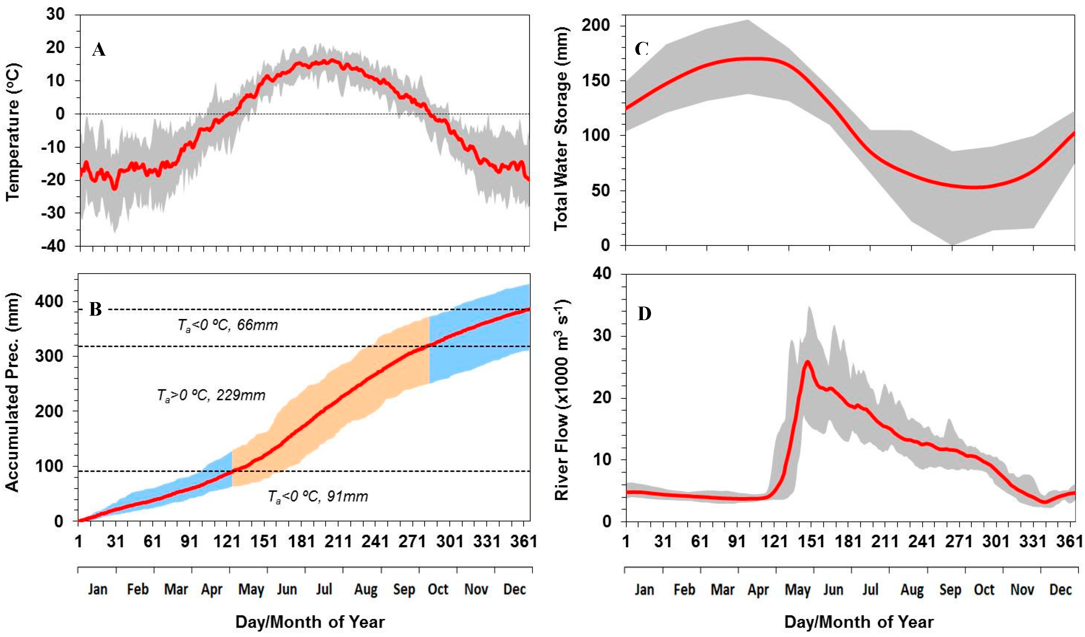
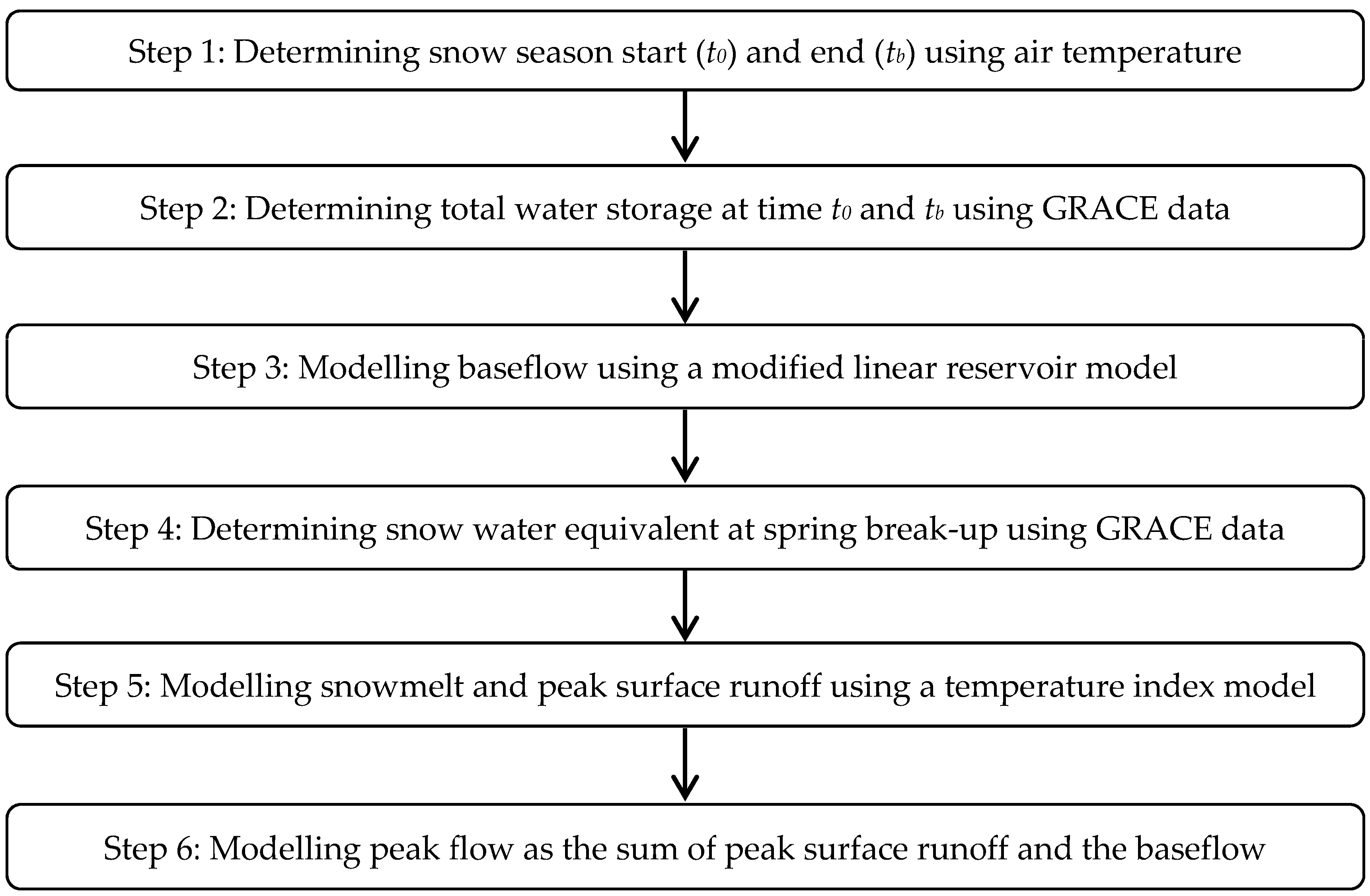
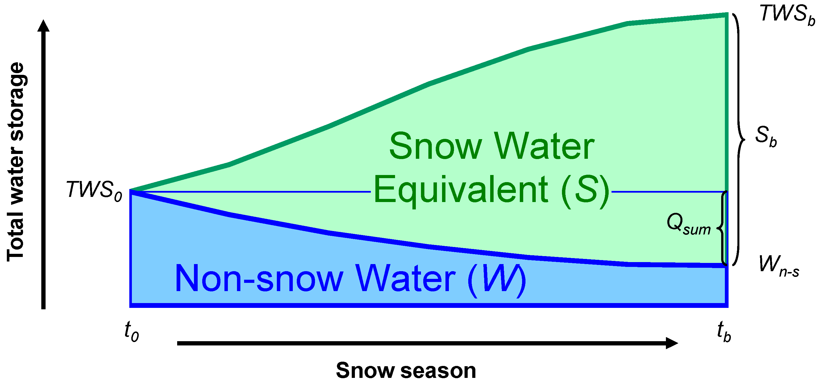
The model gives an average estimate for the start of snow season (t₀) on October 14, and the spring breakup (t_b) on April 29, for the MRB. The average SWE accumulated during this 197-day period is S_b = 160 mm. Note that the SWE is the basin-level amount mainly determined by GRACE, which may differ from an individual site measurement. For comparison, the corresponding total precipitation amount from the GLDAS datasets (see Section 3) for the MRB is 150 mm during this time period. Given a basin-average water loss of 22 mm due to snow sublimation based on Wang et al. [11], the total snow mass during this time period (t₀ to t_b) is 128 mm. The GLDAS-based snow estimate is about 20% lower than the GRACE-based estimate. Snow products such as GLDAS which is benchmarked by in situ measurements likely underestimate the average condition of the entire basin. Many efforts have been made to correct the biases [43,44]. This will be further discussed in Section 5.

The model results show that the MRB has a lump conductivity of a = 1.07 × 10⁻³ day⁻¹ for water discharge, and a threshold value of b = −195.9 mm below which the basin would have no discharge (

Table 1. Baseflow model calibrations and performance evaluations.

n	a (×10−3 Day−1)	B (mm)	r	p	Mean Value (mm)	Mean Absolute Error		Nash Sutcliffe Efficienvy
						(mm)	(%)
12	1.07	−195.9	0.73	<0.007	48.77	2.37	4.9%	0.53

). Compared with the RRB which has a = 0.49 × 10⁻³ day⁻¹ and b = 9.2 mm, the model results suggest that MRB has a relatively high conductivity for water discharge and high water storage state. This is consistent with the facts that the MRB has about 49% of its area as wetland and a large number of lakes which are highly effective in providing large storage capacities and are easy for water discharge. According to Wang et al. [11], annual evapotranspiration for the basin is less than 60% of its annual precipitation, so the basin has a large water surplus for soil and aquifer recharge as well as lake and wetland replenishment to sustain the winter low flows. In contrast, the RRB has a very flat terrain (the slope of the river averages <10 cm·km⁻¹). It also has high evapotranspiration which is close to its precipitation in summer, resulting in a very low water storage state prior to winter. The model results also agree with the observed difference in winter flows, which are as low as 5.8 mm·day⁻¹ for the RRB but as high as 48.8 mm·day⁻¹ for the MRB, as discussed next.

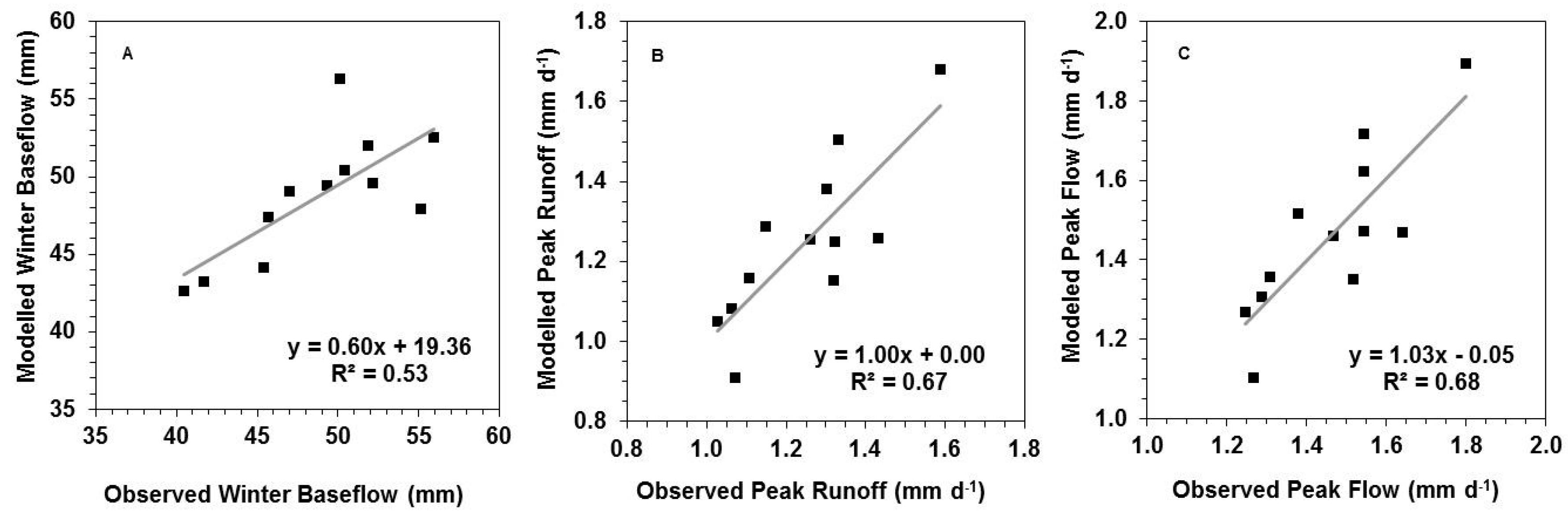
The model performance in estimating winter baseflow for the MRB is given in Table 1 and Figure 5A. Compared to the mean observed baseflow for the study period of 48.8 mm in the snow season, the model has a mean absolute error of MAE = 2.37 mm·day⁻¹, or 4.9% of the observed value. The modelled winter baseflow for the 12 snow years has a correlation coefficient of r = 0.73 with the observed values at a significance level of p < 0.007. The Nash–Sutcliffe model efficiency coefficient for baseflow estimates is NSE = 0.53. The results suggest that the basin winter discharge is primarily driven by its water storage prior to winter. Indeed, surface runoff is minimal in winter due to the lack of liquid precipitation. Water exchange between soil and groundwater is also minimal due to the frozen soil. River flow in winter is thus sustained by groundwater and lake discharge that is controlled by pre-winter storage conditions. Determining groundwater and lake water storage at the basin scale is extremely difficult by traditional methods. The above results underscore the advantages of using GRACE satellite observations in estimating basin water storages and discharge in winter.

The snowmelt model suggests a daily snowmelt rate of α = 17.0 mm per unit of temperature above a base temperature of β = 2.1 °C (

Table 2. Snowmelt and peak surface runoff model evaluation.

n	α (mm·°C−1)	β (°C)	r	p	Mean Value (mm·Day−1)	Mean Absolute Error		Nash Sutcliffe Efficienvy
						(mm·Day−1)	(%)
12	17.0	2.1	0.82	<0.001	1.26	0.10	7.6	0.50

) for the MRB. Compared with the results obtained for the RRB which has α = 18.2 mm per unit temperature and β = 1.0 °C [27], the MRB has a lower heat efficiency and higher base temperature for snowmelt than the RRB. The results are anticipated and they reflect the impacts of other environmental variables on snowmelt that are not included in the model. For example, solar radiation is higher in the RRB than in the MRB, which contributes to the higher snow melting power of temperature in RRB. The relatively small snow amount for the RRB as compared to the MRB (see discussions in Section 5) also results in lower surface albedo due to increased exposure fraction of ground surface [45], which contributes to the more radiative energy absorption and thereafter higher snow melting power per unit temperature in the RRB. Comprehensive and physically based snowmelt models are available and they have the advantages of simulating the integrated impact of all environmental variables (e.g., radiation, humidity, wind speed) on snowmelt [46,47,48], but these kinds of process-based models are data demanding and difficult for operational use over data scarce regions. We use the temperature index model in this study as it needs minimal data input and is easy to implement. In fact, our results demonstrate that the temperature index model performs fairly well, consistent with some other studies [49,50].

The model performance for estimating peak surface runoff Q_runoff is given in Table 2 and Figure 5B. Compared with the observed mean value of 1.26 mm·day⁻¹ over the study period, the model has a mean absolute error of MAE = 0.1 mm·day⁻¹, or 7.6% of the observed value. The modelled peak surface runoff for the 12 snow years has a correlation coefficient of r = 0.82 with the observed values at a significance level of p < 0.001. The Nash–Sutcliffe model efficiency coefficient for surface runoff estimates is NSE = 0.50, slightly lower than that for the baseflow estimates.

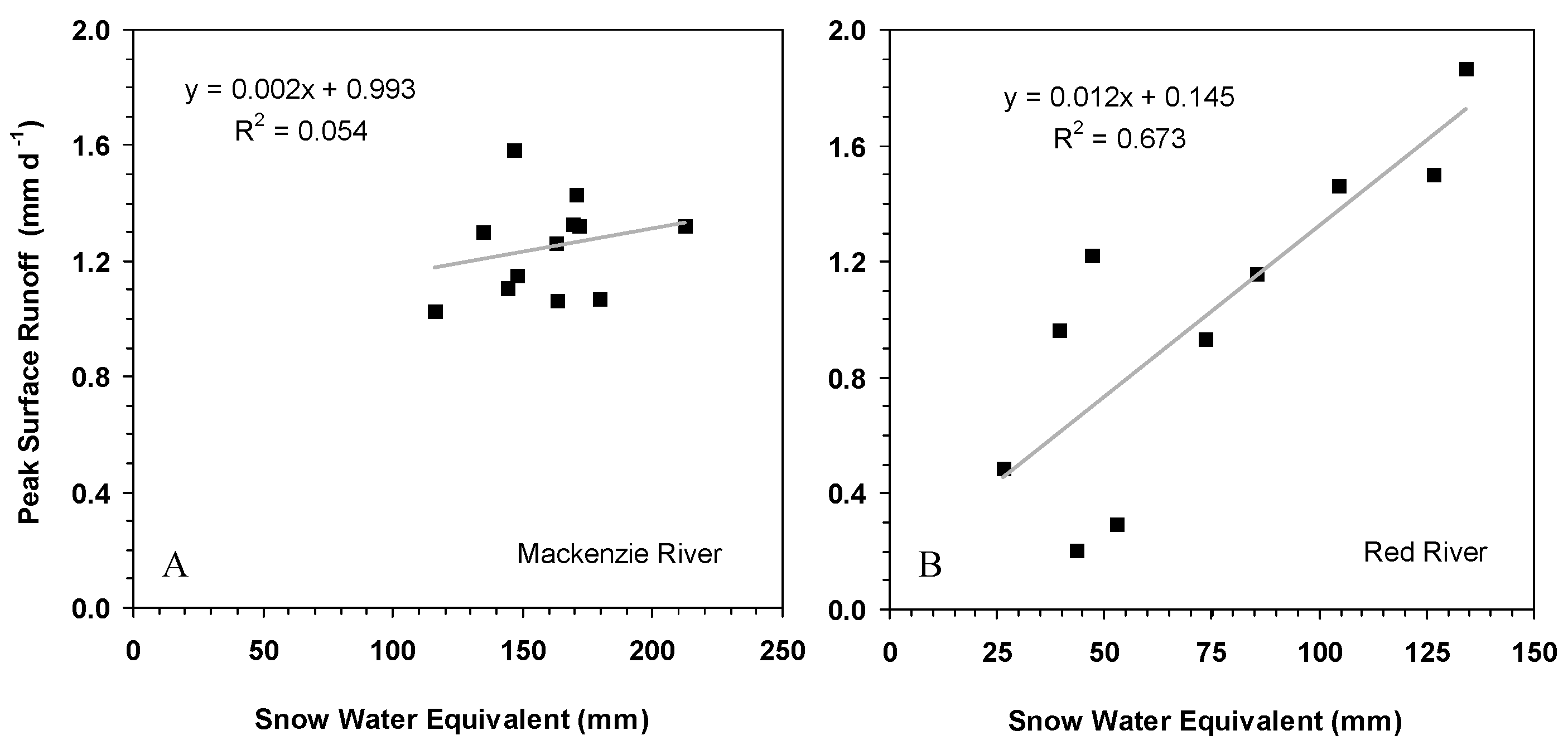
To further examine the relative importance of temperature and snow mass in controlling the peak surface runoff, we analyzed the relationship between S_b and Q_runoff (Figure 6). It was found that Q_runoff had little correlation with S_b. The result indicates that the SWE at spring breakup has little impact on the Q_runoff. Instead, it is the rising temperature during the snowmelt season that mainly drives the interannual variations of Q_runoff for the MRB. In contrast, the correlation between S_b and Q_runoff for the RRB was found to be fairly strong (Figure 6). Specifically, without including T_a, the S_b by itself explained more than two thirds (the coefficient of determination r² = 0.673) of the interannual variations in Q_runoff, suggesting that the major driver for Q_runoff is S_b for the RRB [27]. In a separate study by the British Columbia Ministry of Forests, Lands and Natural Resource Operations [51], the peak flows for the Lower Fraser River (LFR) were analyzed. It was reported that the snow mass contributes about 20%–40%, and the weather factors (mainly temperature) contribute about 60%–80% to the flood risk. The LFR is located in the latitudes between the MRB and the RRB. The above results for the three basins are consistent and appear to suggest that the principal drivers for peak river flows vary with basins. For far north basins, temperature plays a more important role, whereas for southern basins, the amount of snow accumulation plays a more important role in determining the peak river flows or floods.

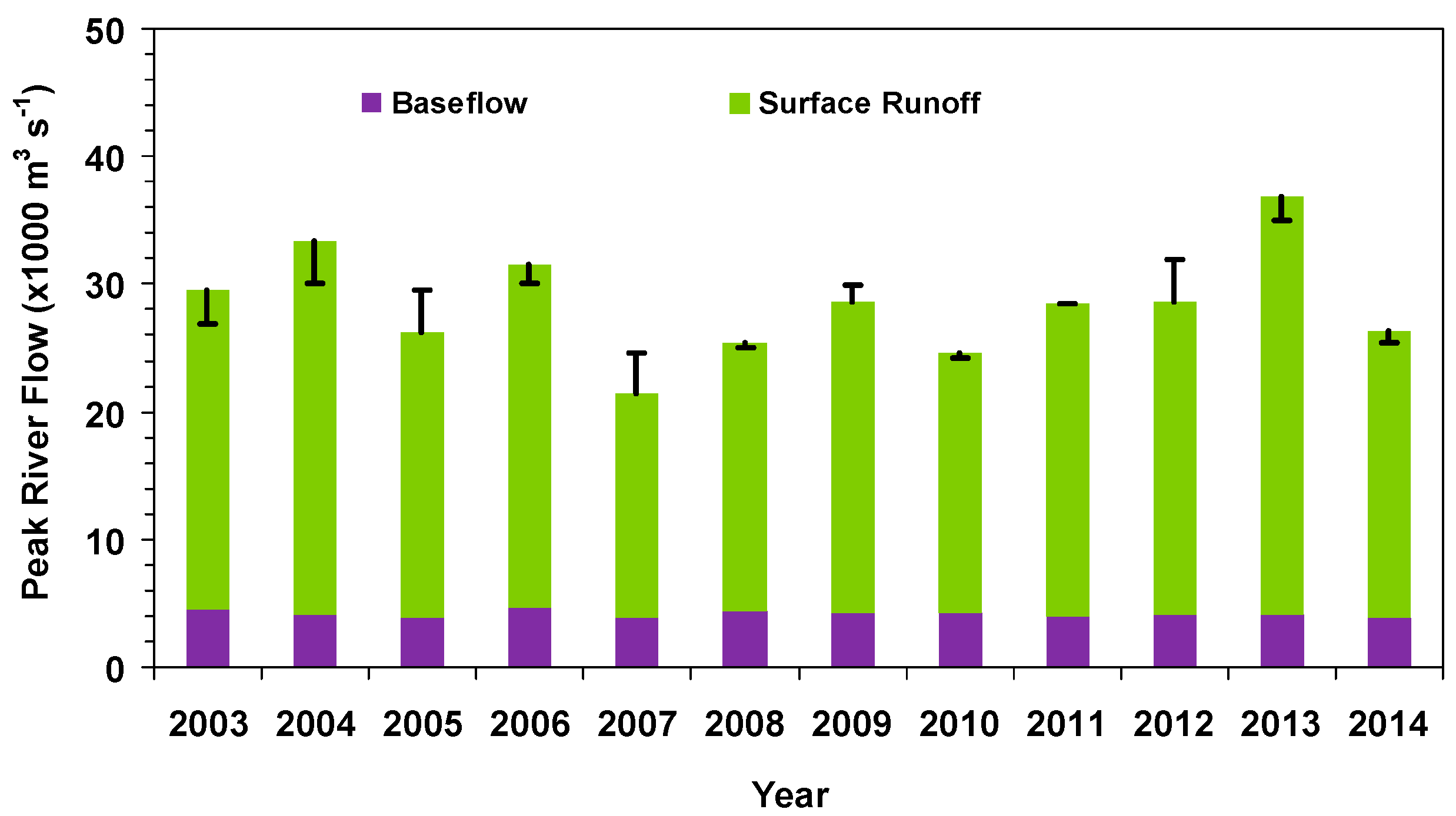
The model performance for estimating peak river flow Q_peak, based on the above results for Q_base and Q_runoff, is given in

Table 3. Peak river flow model evaluation.

n	r	p	Mean Value (mm·Day−1)	Mean Absolute Error		Nash Sutcliffe Efficienvy
				(mm·Day−1)	(%)
12	0.83	<0.001	1.46	0.1	6.5	0.51

and Figure 5C. Compared to the observed mean Q_peak of 1.46 mm·day⁻¹ (28,400 m³·s⁻¹) over the study period, the model result has a mean absolute error of MAE = 0.1 mm·day⁻¹ (1878 m³·s⁻¹), or 6.5% of the mean Q_peak value. The modelled Q_peak for the 12 years has a correlation coefficient of r = 0.83 with the observed values at a significance level of p < 0.001. The Nash–Sutcliffe model efficiency coefficient for peak river flow estimates is NSE = 0.51. Of the peak river flow, 15% is contributed by baseflow and 85% by surface runoff. 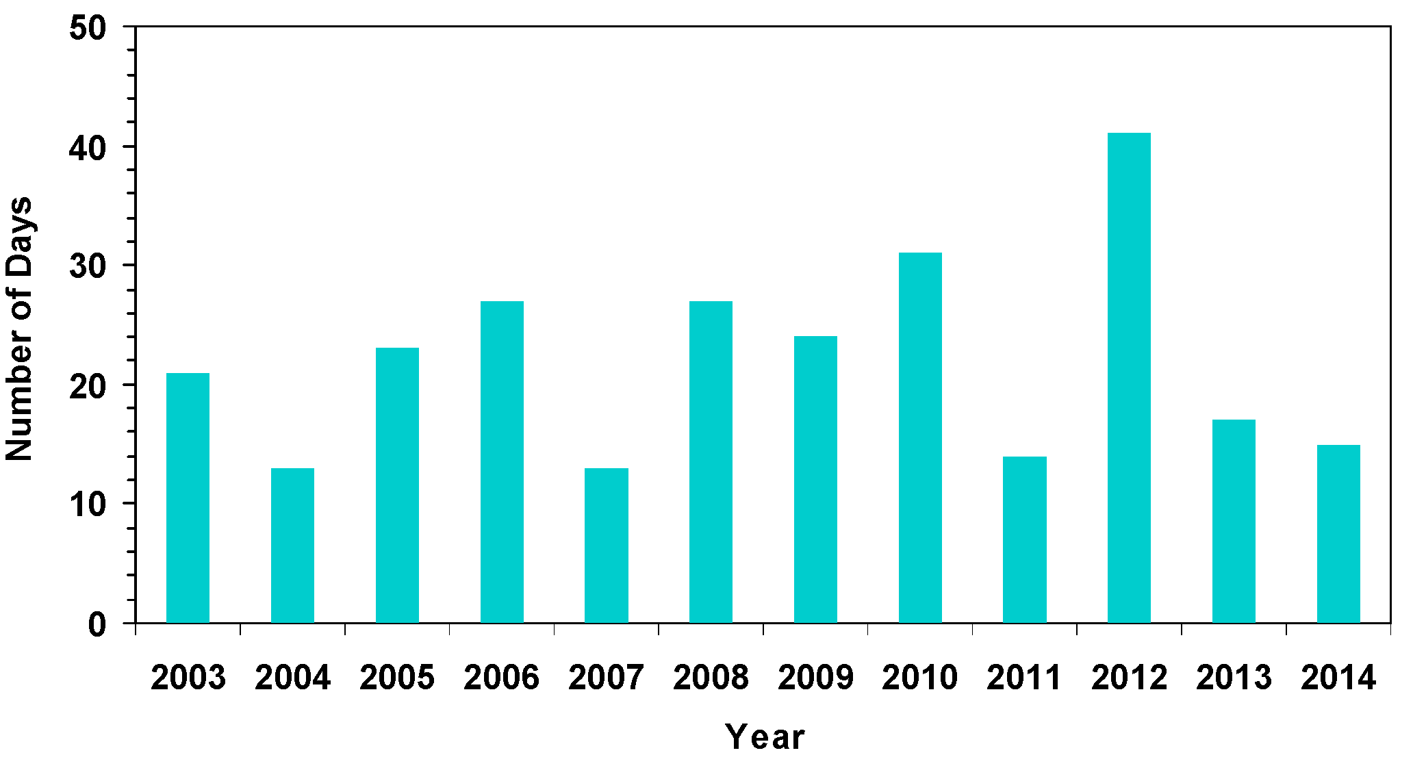As such, the modelling accuracy in Q_base plays a less important role in the modelling accuracy of peak river flows or flood forecasts. Compared to the modelled dates for peak snowmelt, the observed dates for the peak river flow at the station had a delay varying from 13 to 41 days among the 12 years (Figure 7). On average, the delay was about 22 days. The hysteresis indicates the average travel time for the snowmelt water over the basin to reach the hydrometric station. The travel time can be affected by the drainage network density, slope, channel roughness, and soil infiltration characteristics. The large interannual variations of the travel time reflect the impacts of the spring temporal warming process and spatial variations in SWE. For example, a faster increase in spring temperature above 0 °C would result in higher peak flow and a shorter travel time. When more snow is distributed in the downstream region of the watershed, the travel time would also be shorter due to the shorter travel distance.

Results from the LOO-CV show that the 12 models trained using the 12 sets of n−1 (11 years) samples all achieved a correlation coefficient of r > 0.8 with the observed peak river flows at a significance level of p < 0.003, except for the model with year 2013 left-out which had a r = 0.71 and a significance level of p < 0.014. The model forecasts for peak river flows based on the 12 models (Figure 8) had r = 0.72 and MAE = 0.14 mm·day⁻¹, or 9.7% of the observed mean Q_peak value. Compared with the model trained using all the data, the deterioration of the model performance in forecasting the peak river flows from LOO-CV reflects the limited number of data samples due to the short records of the GRACE data. As the GRACE observation continues, and with the follow-up mission of GRACE-FO, it would be necessary to recalibrate the model to refine the parameter values and to increase the model robustness for peak river flow estimates and flood forecasting.

The impact of measurement and leakage error in the GRACE TWS on the model results was investigated by running the model with TWS adjusted by the error either at the pre-winter time (for baseflow) or at the spring breakup (for surface runoff). The impact of the TWS error on the peak river flow estimates was found to be mostly under MAE = 0.06 mm·day⁻¹, or 4% of the mean Q_peak value, which is substantially lower than the modelling error. Compared with that for the RRB [27], the impact of the GRACE TWS error on the modelling results is much smaller for the MRB. This is mainly due to the facts that the error in the GRACE TWS for the MRB is small due to its large area (see Section 3.2). A recent study comparing three GRACE TWS products from mascon and spherical harmonics solutions showed that the differences among GRACE solutions increase with decreasing the basin size by up to a factor of three when going from basins ≥500,000 km² to ≤100,000 km², indicating that the processing approach and uncertainties may be critical for small basins [52]. In addition, the small impact for the MRB is also contributed by the relatively large snow amount and low sensitivity of the peak river flow to S_b for this large basin as discussed above.

5. Discussion

Underestimation of snowfall in cold regions has been long recognized in many studies (e.g., [17,19]) due to the problems as discussed in the Introduction section. This is particularly so for our study region as the available measurement sites, while extremely sparse, are mostly located in valleys or lowlands where people live. Snowfalls at these sites are likely smaller than those at high elevations. Snow products benchmarked by the measurements likely underestimate the average condition of the entire basin. Many efforts have been made to correct the biases [43,44], but they are largely constrained by the difficulties in accurately knowing the amount of snow at the basin-scale. Our study provides a new GRACE-based approach for estimating SWE at the basin-scale. The approach is largely independent of in situ snowfall observations, thus eliminating most of the constraints and uncertainties brought up by the snow gauge measurements and the site-to-basin up-scaling process.

The modelled vs. observed peak river flows have a relatively lower correlation coefficient for the MRB (r = 0.83) than that for the RRB (r = 0.95) obtained in Wang and Russell [27]. This is not surprising as the interannual variations in snow amounts and peak flows of the RRB is much larger than that of the MRB (see discussions below), which provides advantages for more rigorous model calibration and achieves a higher r value. Moreover, the MRB is a much more complicated basin with large spatial heterogeneities in physiographic and climatic conditions than the RRB. As a result, different regions in the MRB were found to have varying flow regimes [33]. For instance, most of the tributary rivers in the southern basin and at low altitudes have peak flows in early May, but in tributary rivers at higher latitudes and high altitudes where snowmelt is delayed, spring peaks occur later. In glacierized basins, the glacier ablation intensifies in the summer which, together with snowmelt at high elevations, prolongs the high flows into summer. Large lakes and reservoirs are highly effective in providing large storage capacities to reduce high flows. The Mackenzie River flow, although exhibiting essentially a subarctic nival regime of snowmelt-induced peak flow, is in fact a combination of many varying flow regimes of its tributary rivers. In contrast, the physiographic and climatic conditions for the RRB are more monotonous and homogeneous, which contribute to the stronger connections between the peak river flows and its peak snowmelt rate modelled for the basin.

The model simulation has moderate NSE values of just above 0.50, r values of above 0.7 (or r² > 0.5), and very small bias (Table 1). The NSE and r values can be judged as satisfactory following the recommendations of Moriasi et al. [53], Santhi et al. [54], and Van Liew et al. [55]. The relative magnitudes of NSE and r varied with modelled variables. For example, the NSE showed a higher value for baseflow than those for peak runoff and river flows, but r values had an opposite pattern. A major reason for the contrasting results is that the baseflow model was calibrated using the least square error while the other two models were calibrated using the r value. Optimizing square errors during model calibration may give high NSE but at the expense of low r, and vice versa. In addition, the variation range of winter baseflow was much smaller than that of peak daily runoff and total flow, which made the r for baseflow over-sensitive to data outliers. The baseflow was likely to have smaller measurement errors than that for the peak runoff and river flow, as the former represents a seasonal total value while the latter represent values at a daily time step. Typically, model simulations tend to be poorer for shorter time steps than for longer time steps [56]. Smaller measurement errors for the total baseflow may provide advantages for achieving higher NSE. Overall, the NSE values for our models are at the lower end of the satisfactory level, partially due to the limited number of data samples and the model calibration approach of optimizing r. The percent biases of our model results showed extremely small values compared with the model evaluation guidelines from other studies (e.g., [53]). This is mainly due to the fact that magnitude of the flows for the Mackenzie River is large, but its interannual variation is very small. Our results suggest that special considerations are required when evaluating the model performance using different statistical parameters. These considerations could include single-event simulation, sample size, quality of measured data, model calibration procedure, evaluation of time step, and project scope and magnitude.

The difference in the main drivers for determining the peak flows of the MRB and RRB is largely due to the difference in their hydroclimatic conditions. The RRB has a mean snow accumulation at spring breakup of 73.3 mm, which is less than half of that for the MRB which is 160.0 mm. On the other hand, the RRB has much larger interannual variations of snow than that for the MRB. The coefficient of variation (CV), or the relative standard deviation (RSD), of the snow amount at spring breakup, which is calculated as the ratio of one standard deviation to the mean, is as high as 49.2% for the RRB. In contrast, the CV is only 14.7% for the MRB. The relatively small amount but large interannual variations of snow in the RRB lead to the fact that years having large snow amount often correspond to severe floods, and years having small snow amount often correspond to very low flows [27]. In contrast, the relatively large and stable snow amounts in the MRB result in the small interannual variations of peak flows and they are mainly determined by the temperature variations during the snowmelt season. Interestingly, this result is found to be consistent with that found for the LFR basin in a separate study [51]. The identification of major drivers for peak flows of different basins is of importance in river flow modelling and flood forecasting.

Some other environmental variables and processes may have significant impacts on the peak river flows over cold regions. For instance, spring floods could be primed by the antecedent conditions of above-average precipitation in the previous fall which fills the available surface and subsurface storage, and by the cold weather prior to the first major snowfall which permits deep freezing of the ground and creates an impermeable surface for the following spring [8]. The water processes during the period from the beginning of snowmelt to the peak flow, such as rain, evapotranspiration, soil thaw-induced surface infiltration or groundwater recharge, and lake storage and river ice dynamics, could have large impacts on the magnitudes of peak flows. The impacts of these processes are not explicitly included in the model and could have contributed to the discrepancies between the model results and the observations. Analysis by Riegger and Tourian [30], however, indicated that the runoff of the MRB during the snowmelt season is mainly determined by the storage discharge, and the impact from net precipitation input (precipitation—evapotranspiration) is close to zero. The soil thaw-induced surface infiltration and groundwater recharge may also have relatively small impacts, as the water flow is mainly from south to north and the lower river sub-basin is usually in a frozen state when the melted water from the south arrives. Moreover, the recharge of groundwater during this time period would lead to an increase in baseflow, which offsets the impact of reduction in surface runoff due to infiltration of the snowmelt water. The calibration of the model using actual peak river flows reduces the impact of this process on the peak river flow modelling. Nevertheless, the impact of the above-mentioned water processes on peak river flows may vary with basins. Further assessment of improvement in model performance by explicitly including these processes in the model needs to be investigated.

This study is mostly based on empirical approaches and focused on characterizing the basin-scale contribution to peak flows using GRACE data of which the footprint is at the scale of 10⁵ km². The approach is not developed to study the detailed hydrological processes within the basin or at the sub-basin scale. Consequently, the model does not address the spatial variations in snow mass, snow break-up date, snowmelt rate, and water flow regimes within the basin. Quantifying the impacts of sub-basin heterogeneity on river flows would require process-based modeling which is beyond the scope of this study. In fact, the above-mentioned sub-basin scale spatial heterogeneities exist even for small basins such as the RRB, as discussed in Wang and Russell [27]. The spatial variations of these variables determine the shape of the flow curve around the peak. The impacts on our results are reflected in the interannual variations and modelling errors. Nevertheless, with the minimal data input requirement and simplified approach, the model has achieved encouraging results on peak river flow or flood forecasting even for a highly heterogeneous basin with very complicated physiographic and climatic conditions. In practice, this GRACE-based approach can be used in combination with other available data and methods to help improve the accuracy in peak flow or flood forecasts.

The GRACE TWS data, which has a monthly temporal resolution, is only used to determine the initial conditions of SWE for the snowmelt model. As the changes of snow mass at the end of the winter season are found to be rather small, the impact of coarse temporal resolution of GRACE data on the model results is largely reduced. Nevertheless, GRACE TWS derived on a higher temporal resolution basis, such as the daily global solutions of Kurtenbach et al. [57] which was found to contain high-frequent temporal gravity field information particular in higher latitudes, or the daily regional solutions of Ramillien et al. [58] which have the advantages of being less smoothed than the global solutions, would better fit our modelling scheme (e.g., the daily time step snowmelt model). The high temporal resolution products are expected to further improve the model performance. This needs to be studied when GRACE daily products are made available.

6. Conclusions

The peak river flow of the MRB is modelled using GRACE satellite observations and temperature data. The model estimates peak river flow by simulating peak surface runoff from snowmelt and the baseflow separately. The results indicate:

(1)

The modelled interannual variations of peak river flows have fairly strong correlations with the observed values at a downstream hydrometric station.

(2)

On average the travel time for the snowmelt water to reach the hydrometric station is about 22 days.

(3)

The major driver for the peak flows of the MRB was found to be air temperature variations in the snowmelt season. In contrast, the snow variations play a more important role in the peak flows for warmer southern basins in Canada.

(4)

Snow mass estimated from the GRACE data was about 20% higher than that from the GLDAS datasets.

(5)

Compared with the RRB, the results indicate that the MRB has relatively high water state and water discharge capability, and low snowmelt efficiency per unit temperature.

This study advances the applications of space-based time-variable gravity measurements in cold region flood forecasting. This GRACE-based model can be readily applied to other cold region basins, and could be particularly useful for regions with minimal data. In practice, it can be used in combination with other available data and methods such as real-time flow data and physically-based flow routing models to help improve the accuracy in river flood forecasting, and develop operation procedures for flood and water resources management.

References

1. Hirabayashi, Y.; Mahendran, R.; Koirala, S.; Konoshima, L.; Yamazaki, D.; Watanabe, S.; Kim, H.; Kanae, S. Global flood risk under climate change. Nat. Clim. Chang. 2013, 3, 816–821. [Google Scholar] [CrossRef]
2. Burton, H.; Rabito, F.; Danielson, L.; Takaro, T.K. Health effects of flooding in Canada: A 2015 review and description of gaps in research. Can. Water Resour. J. 2016, 1–12. [Google Scholar] [CrossRef]
3. Andrews, J. Canada Water Book on Flooding; Environment Canada: Ottawa, ON, Canada, 1993. [Google Scholar]
4. Arnell, N.; Gosling, S. The impacts of climate change on river flood risk at the global scale. Clim. Chang. 2014, 1–15. [Google Scholar] [CrossRef]
5. Church, M. Hydrology and Permafrost with Reference to Northern North America. In Proceedings of the Workshop Seminar on Permafrost Hydrology, Calgary, AB, Canada, 26–28 February 1974; Canadian National Committee, International Hydrological Decade: Ottawa, ON, Canada, 1974; pp. 7–20. [Google Scholar]
6. International Joint Commission. Living with the Red, a Report to the Government of Canada and the United States on Reducing Flood Impacts in the Red River Basin; International Joint Commission: Ottawa, ON, Canada; Washington, DC, USA, 2000; p. 273. [Google Scholar]
7. Yang, D.; Zhao, Y.; Armstrong, R.; Robsinson, D. Yukon River Streamflow Response to Seasonal Snowcover Changes. Hydrol. Process. 2009, 23, 109–121. [Google Scholar] [CrossRef]
8. Rannie, W. The 1997 flood event in the Red River basin: Causes, assessment and damages. Can. Water Resour. J. 2015, 41, 45–55. [Google Scholar] [CrossRef]
9. Goodison, B.E.; Louie, P.Y.T.; Yang, D. WMO Solid Precipitation Measurement Intercomparison; WMO/TD 872; World Meteorological Organization: Geneva, Switzerland, 1998; p. 212. [Google Scholar]
10. Wang, S.; Yang, Y.; Luo, Y.; Rivera, A. Spatial and seasonal variations in evapotranspiration over Canada’s landmass. Hydrol. Earth Syst. Sci. 2013, 17, 3561–3575. [Google Scholar] [CrossRef]
11. Wang, S.; Pan, M.; Mu, Q.; Shi, X.; Mao, J.; Brümmer, C.; Jassal, R.S.; Krishnan, P.; Li, J.; Black, T.A. Comparing evapotranspiration from eddy covariance measurements, water budgets, remote sensing, and land surface models over Canada. J. Hydrometeorol. 2015, 16, 1540–1560. [Google Scholar] [CrossRef]
12. Metcalfe, J.R.; Ishida, S.; Goodison, B.E. A Corrected Precipitation Archive for the Northwest Territories. Mackenzie Basin Impact Study Interim Report No. 2; Environment Canada: Downsview, ON, USA, 1994; pp. 110–117.
13. Hall, D.K.; Riggs, G.A.; Salomonson, V.V.; DiGirolamo, N.E.; Bayr, K.J. MODIS snow-cover products. Remote Sens. Environ. 2002, 83, 181–194. [Google Scholar] [CrossRef]
14. Dong, J.; Walker, J.; Houser, P. Factors affecting remotely sensed snow water equivalent uncertainty. Remote Sens. Environ. 2005, 97, 68–82. [Google Scholar] [CrossRef]
15. Nolin, A.W. Recent advances in remote sensing of seasonal snow. J. Glaciol. 2010, 56, 1141–1150. [Google Scholar] [CrossRef]
16. Hall, D.K.; Riggs, G.A. Accuracy assessment of the MODIS snow products. Hydrol. Process. 2007, 21, 1534–1547. [Google Scholar] [CrossRef]
17. Wang, S.; McKenney, D.W.; Shang, J.; Li, J. A national-scale assessment of long-term water budget closures for Canada’s watersheds. J. Geophys. Res. Atmos. 2014, 119, 8712–8725. [Google Scholar] [CrossRef]
18. Wang, S.; Huang, J.; Li, J.; Rivera, A.; McKenney, D.W.; Sheffield, J. Assessment of water budget for sixteen large drainage basins in Canada. J. Hydrol. 2014, 512, 1–15. [Google Scholar] [CrossRef]
19. Wang, S.; Huang, J.; Yang, D.; Pavlic, G.; Li, J. Long-term water budget imbalances and error sources for cold region drainage basins. Hydrol. Process. 2015, 29, 2125–2136. [Google Scholar] [CrossRef]
20. Tapley, B.D.; Bettadpur, S.; Ries, J.C.; Thompson, P.F.; Watkins, M.M. GRACE measurements of mass variability in the Earth system. Science 2004, 305, 503–505. [Google Scholar] [CrossRef] [PubMed]
21. Sproles, E.A.; Leibowitz, S.G.; Reager, J.T.; Wigington, P.J., Jr.; Famiglietti, J.S.; Patil, S.D. GRACE storage-runoff hystereses reveal the dynamics of regional watersheds. Hydrol. Earth Syst. Sci. 2015, 19, 3253–3272. [Google Scholar] [CrossRef]
22. Jacob, T.; Wahr, J.; Pfeffer, W.T.; Swenson, S. Recent contributions of glaciers and ice caps to sea level rise. Nature 2012, 482, 514–518. [Google Scholar] [CrossRef] [PubMed]
23. Frappart, F.; Ramillien, G.; Famiglietti, J.S. Water balance of the Arctic drainage system using GRACE gravimetry products. Int. J. Remote Sens. 2011, 32, 431–453. [Google Scholar] [CrossRef] [Green Version]
24. Niu, G.-Y.; Seo, K.-W.; Yang, Z.-L.; Wilson, C.; Su, H.; Chen, J.; Rodell, M. Retrieving snow mass from GRACE terrestrial water storage change with a land surface model. Geophys. Res. Lett. 2007, 34, L15704. [Google Scholar] [CrossRef]
25. Frappart, F.; Ramillien, G.; Biancamaria, S.; Mognard, N.M.; Cazenave, A. Evolution of highlatitude snow mass derived from the GRACE gravimetry mission (2002–2004). Geophys. Res. Lett. 2006, 33, L02501. [Google Scholar] [CrossRef]
26. Swenson, S. Assessing High-Latitude Winter Precipitation from Global Precipitation Analyses Using GRACE. J. Hydrometeorol. 2010, 11, 405–420. [Google Scholar] [CrossRef]
27. Wang, S.; Russell, H. Forecasting snowmelt-induced flooding using GRACE satellite data: A case study for the Red River watershed. Can. J. Remote Sens. 2016, 42, 203–213. [Google Scholar] [CrossRef]
28. Woo, M.K. Cold Region Atmospheric and Hydrologic Studies. The Mackenzie GEWEX Experience; Volume 2, Hydrologic Processes; Springer: Heidelberg, Germany, 2008. [Google Scholar]
29. Lorenz, C.; Kunstmann, H.; Devaraju, B.; Tourian, M.J.; Sneeuw, N.; Riegger, J. Large-Scale Runoff from Landmasses: A Global Assessment of the Closure of the Hydrological and Atmospheric Water Balances. J. Hydrometeorol. 2014, 15, 2111–2139. [Google Scholar] [CrossRef]
30. Riegger, J.; Tourian, M.J. Characterization of runoff-storage relationships by satellite gravimetry and remote sensing. Water Resour. Res. 2014, 50, 3444–3466. [Google Scholar] [CrossRef]
31. Sánchez-Murillo, R.; Brooks, E.S.; Elliot, W.J.; Gazel, E.; Boll, J. Baseflow recession analysis in the inland Pacific Northwest of the United States. Hydrogeol. J. 2015, 23, 287–303. [Google Scholar] [CrossRef]
32. Arlot, S.; Celisse, A. A survey of cross-validation procedures for model selection. Stat. Surv. 2010, 4, 40–79. [Google Scholar] [CrossRef]
33. Woo, M.K.; Thorne, R. Streamflow in the Mackenzie Basin, Canada. Arctic 2003, 56, 328–340. [Google Scholar] [CrossRef]
34. Arnell, N.W. Implications of climate change for freshwater inflows to the Arctic Ocean. J. Geophys. Res. 2005, 110, D07105. [Google Scholar] [CrossRef]
35. Wang, S.; Li, J. Terrestrial water storage climatology for Canada from GRACE satellite observations in 2002–2014. Can. J. Remote Sens. 2016, 42, 190–202. [Google Scholar] [CrossRef]
36. Li, J.; Wang, S.; Zhou, F. Time Series Analysis of Long-term Terrestrial Water Storage over Canada from GRACE Satellites Using Principal Component Analysis. Can. J. Remote Sens. 2016, 42, 161–170. [Google Scholar] [CrossRef]
37. Prowse, T.; Shrestha, R.; Bonsal, B.; Dibike, Y. Changing spring air temperature gradients along large northern rivers: implications for severity of river-ice floods. Geophys. Res. Lett. 2010, 37, 201–215. [Google Scholar] [CrossRef]
38. Yang, D.; Shi, X.; Marsh, P. Variability and extreme of Mackenzie River daily discharge during 1973–2011. Quat. Int. 2014. [Google Scholar] [CrossRef]
39. Swenson, S.C. GRACE Monthly Land Water Mass Grids NETCDF RELEASE 5.0; Ver. 5.0; PO.DAAC: Pasadena, CA, USA, 2012. [Google Scholar]
40. Swenson, S.C.; Wahr, J. Post-processing removal of correlated errors in GRACE data. Geophys. Res. Lett. 2006, 33, L08402. [Google Scholar] [CrossRef]
41. Landerer, F.W.; Swenson, S.C. Accuracy of scaled GRACE terrestrial water storage estimates. Water Resour. Res. 2012, 48, W04531. [Google Scholar] [CrossRef]
42. Wahr, J.; Swenson, S.; Velicogna, I. Accuracy of GRACE mass estimates. Geophys. Res. Lett. 2006, 33, L06401. [Google Scholar] [CrossRef]
43. Woo, M.K.; Heron, R.; Marsh, P.; Steer, P. Comparison of weather station snowfall with winter snow accumulation in High Arctic basins. Atmos. Ocean 1983, 21, 312–325. [Google Scholar] [CrossRef]
44. Yang, D.; Kane, D.; Zhang, Z.; Legates, D.; Goodison, B. Bias-corrections of long-term (1973–2004) daily precipitation data over the northern regions. Geophys. Res. Lett. 2005, 32, L19501. [Google Scholar] [CrossRef]
45. Wang, S.; Davidson, A. Impact of climate variations on surface albedo of a temperate grassland. Agric. For. Meteorol. 2007, 142, 133–142. [Google Scholar] [CrossRef]
46. Wang, S.; Trishchenko, A.P.; Sun, X. Simulation of canopy radiation transfer and surface albedo in the EALCO model. Clim. Dyn. 2007, 29, 615–632. [Google Scholar] [CrossRef]
47. Wang, S. Simulation of evapotranspiration and its response to plant water and CO2 transfer dynamics. J. Hydrometeorol. 2008, 9, 426–443. [Google Scholar] [CrossRef]
48. Zhang, Y.; Wang, S.; Barr, A.G.; Black, T.A. Impact of snow cover on soil temperature and its simulation in the EALCO model. Cold Reg. Sci. Technol. 2008, 52, 355–370. [Google Scholar] [CrossRef]
49. Li, L.; Simonovic, S.P. System dynamics model for predicting floods from snowmelt in North American prairie watersheds. Hydrol. Process. 2002, 16, 2645–2666. [Google Scholar] [CrossRef]
50. Griessinger, N.; Seibert, J.; Magnusson, J.; Jonas, T. Assessing the benefit of snow data assimilation for runoff modeling in alpine catchments. Hydrol. Earth Syst. Sci. Discuss. 2016. [Google Scholar] [CrossRef]
51. British Columbia Ministry of Forests, Lands and Natural Resource Operations. Flow Forecasting for the Lower Fraser River (from Hope to the Ocean); Prepared by River Forecast Centre, B.C. Ministry of Forests, Lands and Natural Resource Operations, Water Management Branch; 2012. Available online: http://bcrfc.env.gov.bc.ca/freshet/lower_fraser/Flow%20Forecasting%20for%20the%20Lower%20Fraser%20River.pdf (accessed on 9 March 2017).
52. Scanlon, B.R.; Zhang, Z.; Save, H.; Wiese, D.N.; Landerer, F.W.; Long, D.; Longuevergne, L.; Chen, J. Global evaluation of new GRACE mascon products for hydrologic applications. Water Resour. Res. 2016, 52. [Google Scholar] [CrossRef]
53. Moriasi, D.N.; Arnold, J.G.; van Liew, M.W.; Bingner, R.L.; Harmel, R.D.; Veith, T.L. Model evaluation guidelines for systematic quantification of accuracy in watershed simulations. Trans. ASABE 2007, 50, 885–900. [Google Scholar] [CrossRef]
54. Santhi, C.; Arnold, J.G.; Williams, J.R.; Dugas, W.A.; Srinivasan, R.; Hauck, L.M. Validation of the SWAT model on a large river basin with point and nonpoint sources. J. Am. Water Resour. Assoc. 2001, 37, 1169–1188. [Google Scholar] [CrossRef]
55. Van Liew, M.W.; Arnold, J.G.; Garbrecht, J.D. Hydrologic simulation on agricultural watersheds: Choosing between two models. Trans. ASAE 2003, 46, 1539–1551. [Google Scholar] [CrossRef]
56. Engel, B.; Storm, D.; White, M.; Arnold, J.G. A hydrologic/water quality model application protocol. J. Am. Water Resour. Assoc. 2007, 43, 1223–1236. [Google Scholar] [CrossRef]
57. Kurtenbach, E.; Eicker, A.; Mayer-Gürr, T.; Holschneider, M.; Hayn, M.; Fuhrmann, M.; Kusche, J. Improved daily GRACE gravity field solutions using a Kalman smoother. J. Geodyn. 2012, 59–60, 39–48. [Google Scholar] [CrossRef]
58. Ramillien, G.; Frappart, F.; Gratton, S.; Vasseur, X. Sequential estimation of surface water mass changes from daily satellite gravimetry data. J. Geod. 2015, 89, 259–282. [Google Scholar] [CrossRef]
Figure 1. Map for the the Mackenzie River Basin (MRB) and the hydrometric station for river flow measurement (A), and its location in Canada’s landmass (B). The Red River Basin (RRB) is also shown on the map of Canada.
Remotesensing 09 00256 g001
Figure 2. Flowchart for the modelling processes.
Remotesensing 09 00256 g002
Figure 3. Diagram illustrating snow accumulation (S) and non-snow water (W) discharge for the Mackenzie River Basin in snow cover season. t0 and tb: start and breakup time of the snow season; TWS0 and TWSb: basin total water storage (S + W) at time t0 and tb; Wn-s: non-snow water at time tb; Sb: Snow Water Equivalent at tb; Qsum: accumulated basin water discharge in the snow season.
Remotesensing 09 00256 g003
Figure 4. Hydroclimate characterization for the Mackenzie River Basin during the study period of 2003–2014. (A) Daily air temperature; (B) Accumulated precipitation during a year (blue represents snow; orange represents rain); (C) Total water storage change from the Gravity Recovery and Climate Experiment (GRACE) satellite observations; and (D) Daily river flow measured at the hydrometric station. More details on the data sources can be found in Section 3.2. Red lines in all panels represent the mean values over the study period of 2003–2014. Shadowed areas represent the maximum and minimum variation ranges within the study years.
Remotesensing 09 00256 g004
Figure 5. Comparison of model results for the Mackenzie River Basin. (A): modeled vs. observed total baseflow in winter; (B): modeled vs. observed daily peak surface runoff; (C): modeled vs. observed daily peak river flow.
Remotesensing 09 00256 g005
Figure 6. Comparison of the Mackenzie River Basin (A) vs. the Red River Basin (B) for the relationships between peak surface runoff (Qrunoff) and snow water equivalent at spring break-up (Sb).
Remotesensing 09 00256 g006
Figure 7. The time difference for the study period of available GRACE data between the dates for modeled peak snowmelt and observed peak river flow at the hydrometric station. The average is a 22 day offset.
Remotesensing 09 00256 g007
Figure 8. The leave-one-out cross-validation (LOO-CV) results for peak river flow forecasts. The error bar is the difference between forecasted and observed peak river flows for each year.
Remotesensing 09 00256 g008