Glacier Mass Loss during the 1960s and 1970s in the Ak-Shirak Range (Kyrgyzstan) from Multiple Stereoscopic Corona and Hexagon Imagery

Abstract

Comprehensive research on glacier changes in the Tian Shan is available for the current decade; however, there is limited information about glacier investigations of previous decades and especially before the mid 1970s. The earliest stereo images from the Corona missions were acquired in the 1960s but existing studies dealing with these images focus on single glaciers or small areas only. We developed a workflow to generate digital terrain models (DTMs) and orthophotos from 1964 Corona KH-4 for an entire mountain range (Ak-Shirak) located in the Central Tian Shan. From these DTMs and orthoimages, we calculated geodetic mass balances and length changes in comparison to 1973 and 1980 Hexagon KH-9 data. We found mass budgets between −0.4 ± 0.1 m·w.e.a⁻¹ (1964–1980) and −0.9 ± 0.4 m·w.e.a⁻¹ (1973–1980) for the whole region and individual glaciers. The length changes, on the other hand, vary heterogeneously between +624 ± 18 m (+39.0 ± 1.1 m·a⁻¹) and −923 ± 18 m (−57.7 ± 1.1 m·a⁻¹) for 1964–1980. An automation of the processing line can successively lead to region-wide Corona data processing allowing the analysis and interpretation of glacier changes on a larger scale and supporting a refinement of glacier modelling.

1. Introduction

Tian Shan glaciers are important for the water cycle of the arid Central Asian regions [1,2] and experienced a pronounced mass loss in the outer ranges and only moderate mass loss in the Central Tian Shan [3,4]. Within the Khan Tengri-Jengish Chokusu region, the Central Tian Shan contains the most glacierised region within the entire Tien Shan. The Ak-Shirak massif (~40 × 40 km²), located at the western margin of the Central Tian Shan (sometimes also considered Inner Tian Shan, Figure 1), was covered by more than 150 glaciers with an area of ~380 km² in 1964 and showed the highest glacier mass loss in the Central Tian Shan [5]. In the Ak-Shirak area, which is also well known for surge-type glaciers [6,7], an important part of the accumulation process takes place in summer [8]. At the Tian Shan meteorological station (3614 m a.s.l.), the mean annual temperature between 1964 and 1980 was −7.5 °C and the annual precipitation was 321 mm, from which 85% occurred between April and October. Thus, there is a strong dependency on the amount of precipitation at low summer temperatures. Hence, the observed negative precipitation trend especially in the summer months [4] and a general temperature rise [9] might be responsible for the negative glacier mass budgets. To better link climate change to glacier melting, a long observation period of glacier changes is favourable.

Previous research on Ak-Shirak glaciers, based on topographic maps, tachymetric measurements and aerial photographs found a mean mass loss of 0.20 ± 0.10 m·w.e.a⁻¹ for the 1943 to 1977 period, which cumulates to almost 30% of the estimated total ice volume [10,11]. Mass loss rates of 0.51 ± 0.25 m·w.e.a⁻¹ were found for the following period from 1975 to 1999 [5]. This study and few others [12,13,14] used Hexagon satellite data for their analysis and illustrated the high potential of the declassified data.

The satellite reconnaissance imagery of the Hexagon and Corona missions, acquired as part of the Key Hole program of the United States of America, was declassified in the years 1995, 2002 and 2013 [2,15]. With the start of the KH-4 program in 1962, the Corona system offers stereo capabilities and therefore the possibility to compute digital terrain models (DTMs). The Corona mission tasks were followed by the Hexagon missions in 1971, also offering stereo and sometimes even tri-stereo capabilities. These two programs open the door to the extraction of large amounts of geospatial data that can be used for historical analysis of processes of interest.

Little research has been done in this field especially on Corona data. Beck et al. [16] and Altmaier and Kany [17] rectified Corona imagery in low elevated terrain without ice and snow cover with an accuracy of 5–8 m and 10 m, respectively. Further studies mainly focussed on 2D changes [18,19,20] and did not exploit the full potential of the data for 3D observations and processing. Focusing on small area or single glaciers only, previous research used the stereoscopic capabilities of declassified Corona imagery to extend existing mass budget series back in time [21,22,23,24]. A recent study on Corona data [24] using KH-4B imagery resulted in a DTM with an accuracy of 4 m for an area of ~3 × 1.5 km². They [21,22,23,24] found negative geodetic mass budgets for the Khumbu Himalaya and the Kyrgyz Ala-Too for several periods based on Corona KH-4 data.

In contrast, the research on processing Hexagon imagery made definite progress by studies of Pieczonka and Bolch [5] processing the data partially automated for a glacierised area of ~5000 km². One step further, Maurer and Rupper [25] developed an automated processing line for Hexagon DTM generation and determined glacier mass budgets for a sample of glaciers in the Bhutanese Himalaya [12].

The objective of the present study is therefore to present a workflow for Corona imagery DTM generation for glacier change studies focusing on entire Ak-Shirak range (Figure 1a). Furthermore, previous studies investigated glacier mass budgets [5,10,26] and allow evaluation of our results generated using declassified data only. Additionally, short-term glacier changes are studied to investigate surge-type characteristics and elevation change patterns not detectable in long-term studies considering several decades.

2. Materials and Methods

2.1. Data

2.1.1. Corona and Hexagon Imagery

The Corona reconnaissance satellite program operated between 1959 and 1972 as part of the US Key Hole program [27]. The main objective was to obtain information about the territory of the former Soviet Union in the beginning and all restricted regions worldwide later on. Consequently, the coverage in Central Asia is dense with several image series per year for most areas (we found >300 scenes for the Ak-Shirak massif).

The KH-4 mission satellites were the first to acquire stereo imagery from space. For that purpose, they carried two panoramic cameras tilted, respectively, 15° forward (FWD) and backward (AFT) at an orbit of ~200 km. The cameras are characterised by a focal length of 602.6 mm, a fixed aperture width of 5.265°, a pan angle of 71.16° and a light sensitive panchromatic film with a resolution between 50 and 160 lines/mm [27,28]. This results in scenes with a ground coverage between 14 × 188 km² and 17 × 232 km² in flat terrain at sea level [27,28]. Nearly every ground point is covered by two images with a nadir resolution between 1.8 m and 7.6 m [15,17]. Due to the panoramic camera system, the scenes are highly distorted in several directions (Figure 2) [29]. We processed the scenes using the Remote Sensing Software Package Graz (RSG) Version 7.46.17, which includes the unique unpublished Corona KH-4/A/B camera model. The main differences between the missions are the orbital height above the earth surface and the different film resolutions of the three different satellites resulting in variable ground resolutions while the camera specifics are similar.

In this study, we used scenes from the KH-4A mission 1014 acquired in November 1964, which provides the first usable dataset for the Ak-Shirak range we could find. Besides cloud and snow coverage, the dependency on the solar altitude, which is reinforced through the camera tilt, needs to be considered in terms of image selection. Each KH-4A scene covers an area of ~17 × 232 km² with a nadir ground resolution between 2.7 m and 7.6 m [27,28]. The Ak-Shirak is located close to the centre of the scenes (Figure 3), which results in comparably low image distortions. All Corona images were manually scanned by USGS with a scan resolution of 14 μm and provided in four parts with a varying overlap 20%–30% of the single parts.

The KH-9 Hexagon Mapping Camera (MC) operated from 1973 until 1980. The MC used the same film as the KH-4 missions capturing images but had a much larger ground coverage of about ~125 × 250 km² [31,32]. The existence of 1058 reseau crosses per scene in Hexagon imagery is extremely helpful to provide a basis for geometric rectification [32]. The Hexagon images used are scanned with a scan resolution of 14 μm in two parts with ~13% overlap. All scene parts, Hexagon as well as Corona, were assembled before further processing to restore the original image geometry. We used Hexagon KH-9 imagery (Figure 3) from 1980 for DTM generation and orthophoto generation, glacier mapping, and to illustrate the potential of the data. The KH-9 scenes from 1973 were used for the data quality potential illustration. The KH-9 1973 DTM (co-registered to SRTM) was provided as a fully processed dataset (cf. [5]). It was used for co-registration since the resolution is higher than the SRTM. Furthermore, it was used for mass budget calculation purposes as well as the corresponding outlines for length change assessment.

2.1.2. Reference Data

We used the panchromatic bands of Landsat 7 ETM+ and Landsat 8 OLI for georeferencing, as no ground control points were available (

Table 1. Input datasets.

Sensor	Date	Scene ID/Path-Row	Spatial Resolution	Usage
Corona KH-4A	18/11/1964	DS1014-2134DA088	7.6 m	DTM generation; Mass budget; Glacier mapping
		DS1014-2134DA089
		DS1014-2134DA090
		DS1014-2134DF084
		DS1014-2134DF085
		DS1014-2134DF086
Hexagon KH-9 DTM	31/07/1973	DZB1206-500069L010001	7.6 m (DTM 25 m)	Mass budget; Co-registration
		DZB1206-500069L011001
		DZB1206-500069L012001
Hexagon KH-9	21/08/1980	DZB1216-500277L021001	7.6 m	DTM generation; Mass budget; Glacier mapping
		DZB1216-500277L022001
		DZB1216-500277L023001
SRTM	11/02/2000	n41_e076	~30 m	Vertical reference
		n41_e077
Landsat 7 ETM+	17/08/1999	LE71480301999229EDC00	15 m	Geocoding
	19/08/2000	LE71480312000232SGS00
	09/09/1999	LE71490311999252SGS00
	29/10/2000	LE71490302000303SGS00
Landsat 8 OLI	02/10/2013	lc81480312013275lgn00	15 m	Geocoding

). Shuttle Radar Topography Mission (SRTM) data (~30 m, 1-arc s, v3) formed a rough basis for disparity prediction information (Section 3.2) during the DTM generation process (Table 1) and was used as vertical reference for ground control points (GCPs). The reported horizontal and vertical accuracy of the SRTM data is below 20 m and 16 m, respectively [33]. Furthermore Berthier et al. [34] found elevation variances of +7 m up to −10 m for alpine regions in the French Alps. All datasets were downloaded from EarthExplorer [35].

2.2. Methods

2.2.1. DTM Generation

RSG, developed by the Joanneum Research Graz, was used for Corona DTM generation. The workflow follows a basic photogrammetric approach as shown in Figure 4. Since the study region is located in the centre of the scenes, we created image subsets of 18,001 by 3801 pixel (px). To determine the orientation parameters of the camera, we manually measured between 20 GCPs for scene DF084 and 40 GCPs for scene DF086 (

Table 2. Geometric parameter adjustment results for absolute orientation. x, parallax across flight direction; y, parallax in flight direction.

Image	No. of GCPs	RMS Res X	RMS Res Y
DA88	24	2.94	2.80
DA89	35	2.82	2.88
DA90	36	2.86	2.04
DF84	20	2.35	3.14
DF85	24	2.56	2.65
DF86	40	2.99	2.78

) with the integrated point measurement tool of RSG. The RSG software provides a Corona-adapted image distortion model, which is essential to set up a geometric model. The model is based on a classical photogrammetric collinearity equation with a modification concerning the panoramic geometry. With the help of the GCPs, the model is optimised and leads to maximum residuals of ~3 px (Table 2). The specific Corona camera input parameter values are listed in

Table 3. Default scene parameter values. Ω, viewing angle across flight direction; φ, forward and backward camera tilt; κ, flight direction (0° = east).

Scene	Omega (ω)	Phi (φ)	Kappa (κ)	Flying Height (m)	Focal Length (mm)	Size (px)
FWD	0°	15°	61°	200,000	609.602	18,001 × 3801
AFT		−15°

. Successively, the corresponding scenes were combined into stereo image blocks.

For the main step of DTM generation, we registered the two stereo partner images to each other. RSG provides a matching-based automated Tie-Point (TP) measurement tool to generate TPs for all stereo pairs, which forms the basis for the image registration. The tool uses the Foerstner operator [36] to detect most significant points of previously generated image sub-windows. The collected points are matched to the corresponding scene. We used the forward scenes for the point detection as they are mostly of higher contrast for this scene series.

Table 4. Geometric parameter adjustment results for relative orientation. x, parallax across flight direction; y, parallax in flight direction.

Stereo Pair	Tie Points	RMS Res (px)		MIN Res (px)		MAX Res (px)
		x	y	x	y	x	y
DA88_DF84	131	14.81	1.44	−34.76	−3.11	32.44	3.02
DA88_DF85	75	5.16	0.31	−8.40	−0.86	12.21	0.65
DA89_DF85	139	24.68	2.18	−54.84	−4.87	51.56	4.79
DA89_DF86	108	31.25	1.31	−74.55	−2.85	76.14	2.90
DA90_DF86	149	25.25	1.92	−55.60	−4.31	62.53	4.63

shows the intermediate geometric adjustment results with an expected high parallax across and a low parallax in flight direction. Due to a parallax of more than one pixel, we had to use a polynomial rectification registration approach instead of an epipolar registration. This process, however, leads to a higher processing time and lower quality owing to a two-dimensional point search and higher probability of wrongly assigned pixels. Thereby, the polynomial approach results in a relatively small search window for the matching process while an epipolar registration would lead to corresponding points on epipolar lines and thus a much faster and more stable one-dimensional matching process.

To optimise the processing time and the robustness of the matching, we calculated matching disparity predictions in both directions based on the registered geometric image models and SRTM data. Due to the generated matching prediction raster, we were able to minimise the extent of the matching search window. This led to two major tweaks: the processing time of this approach is significantly reduced (~4 times faster) and the opportunity of wrongly assigned pixels is diminished. The matching was performed in three pyramid-based levels with two different search window extents of 5 × 11 px (top level) and 5 × 5 px (2nd and 3rd level). The result is a four-band disparity raster, which depicts low disparities in column direction (band 1) and various disparities in line direction (band 2) caused by the camera viewing angles (Figure 5). Bands 3 and 4 contain feature and backmatching distance information, respectively.

We used a threshold filter based on the disparity map bands 3 and 4 to eliminate mismatched regions. The values of the quality and backmatching threshold were defined considering that the quality values of the notably mismatched regions are higher than the local minimum of the corresponding band 3 histogram curve (Figure 6). Regarding the backmatching distance, the focused regions show the same values of ~1 px for all matchings we run. The histogram curve (Figure 6) shows the already manually observed behaviour and has a major peak at ~1. Consequently, we set the backmatching distance threshold to 0.99. Most regions assigned as mismatched regions were snow covered or shadowed regions with low contrast. The interpolation of mismatched stable terrain sections could lead to delusive high DTM elevation inaccuracies. Therefore, in terms of DTM co-registration, interpolation of these regions was not applied here.

The KH-9 DTM for 1980 was generated from the stereo pair using ERDAS Imagine 2014 Photogrammetry Suite. This includes the elimination of internal distortions using the reseau crosses following Pieczonka et al. [14]. We chose the frame camera model with a fixed focal length of 30.5 cm and flying height of 170 km. We calculated the reference positions of the reseau crosses assuming that the distance between two crosses is 1 cm (714.28 px) to solve the interior orientation. The coordinates of all four fiducial points were measured manually defining the principal point in the image centre (0,0). We collected 29 GCPs using distinct topographic terrain features like river crossings or mountain ridges from Landsat 7 ETM+ imagery (L1T processing level) with SRTM as a vertical reference. Afterwards, 29 TPs were generated automatically using the Leica Photogrammetry Suite. The resulting RMS error of triangulation was 0.982 px.

To align all DTMs, we eliminated the spatial trend using a second order trend surface based on non-glacierised pixels on flat terrain <15° [21,37]. Due to the tilts and shifts of the Corona and Hexagon DTMs, we got the best results with this method. This was followed by the co-registration after Nuth and Kääb [38]. For co-registration, we used the 1973 Hexagon DTM as master DTM taking only slopes between 0° and 30° into account. The co-registration process for each DTM converged after eight iterations maximum, when the remaining horizontal offset was less than 1 m. Finally, we created a DTM mosaic of all single Corona DTMs blending (mean value) overlapping parts (~8% per DTM, 4% on each side).

2.2.2. Glacier Mapping and Length Changes

Glacier outlines for this area generated from the 1973 Hexagon KH-9 served as baseline data (cf. [5]). These outlines were manually adjusted using the generated 1964 and 1980 orthoimages assuming stable accumulation regions.

Glacier length changes were calculated for the selected glaciers (Figure 1). Therefore, we placed parallel lines over the glacier tongue in flow direction and calculated the mean length difference of the lines between outlines of two years to get the final length change (cf. [20,39]).

2.2.3. Data Gap/Outlier Handling

We used an elevation dependent pixel based approach assuming a nonlinear decreasing variance of elevation differences from the ablation towards the accumulation region [40,41] to eliminate outliers on glacierised terrain [5]. Equations (1) to (3) describe the eliminating principle of the glacier-covered regions in dependence of terrain elevation [5].

$$\Delta h_{max}=c_{STD}\times ST{D}_{Glac},$$

(1)

$$c_{STD}=5-5\tanh (2\pi -10w),$$

(2)

$$w=\frac{\left(h_{max}-h_{min}\right)}{h_{Glac}},$$

(3)

where $\Delta h_{max}$ is the maximum thickness difference; $c_{STD}$ is the weighting coefficient; $ST{D}_{Glac}$ is the overall standard deviation of glacier $\Delta h$; $w$ is the normalised glacier pixel elevation; $h_{max}$/$h_{min}$ is the maximum/minimum glacier elevation; and $h_{Glac}$ is the pixel glacier elevation.

As Equation (3) considers the maximum elevation range within the study region, we had to adapt it for the Ak-Shirak area. The weighting coefficient ${\mathit{c}}_{\mathit{S}\mathit{T}\mathit{D}}$ is determined with 0.2 (min) in the highest (5050 m a.s.l.) and 9.5 (max) in the lowest (2850 m a.s.l.) regions. The coefficient range must be that large to take surge-type glaciers into account, for which the Ak-Shirak massif is well-known [6,7]. Furthermore, we filtered both analysed periods with the same equation, which was only possible because the standard deviation difference (41 and 49) roughly represents the time difference. Due to issues with data outliers in the ELA (equilibrium line altitude) and accumulation areas, we further set the threshold of surface elevation rise in the ablation regions to +10 m (for none-surge-type glaciers) and changes in the accumulation region to ±10 m.

Afterwards, we filled all data gaps in the ablation regions using ordinary kriging interpolation (64–73: 15%; 73–80: 10%; 64–80: 11% of the entire ablation area). As the main surface elevation differences are expected in the ablation region and no significant surface elevation changes in the accumulation region are expected, we filled data gaps with 0 (64–73: 86%; 73–80: 79%; 64–80: 87% of the entire accumulation area) [12,40]. These interpolations involve data gaps from the matching process as well as previous DTM filtering.

2.2.4. Accuracy Assessment

In order to evaluate the glacier surface elevation differences, we calculated the uncertainties following the approach of Gardelle et al. [42] and estimated the mean error $E_{\Delta h}$ over the elevation bands of stable terrain of the DTM difference image. Following Equation (4), we calculated the errors for each elevation band within a buffer of 1 km around the glacierised regions without terrain >30°.

$$E_{\Delta h}=\frac{E_{\Delta h_i}}{\sqrt{N_{eff}}},$$

(4)

where $E_{\Delta h_i}$ is the standard deviation of mean elevation change for each band i = 1, ..., n; and $N_{eff}$ is the number of effectively included pixel without autocorrelation.

$$N_{eff}=\frac{N_{tot}\times R}{2d},$$

(5)

where $N_{tot}$ is the total number of elevation difference pixel in certain elevation band; $R$ is the difference raster resolution in m; and $d$ is the autocorrelation distance in m.

To determine the autocorrelation distance $d$, we used Moran’s I autocorrelation index on stable terrain within the 1 km buffer. The autocorrelation distances for the entire massif are 318 m and for the individually observed glaciers between 150 m and 430 m. For each glacier, we used its individual stable terrain autocorrelation distance within the 1 km buffer. Finally, we weighted each elevation band error by the hypsometry of the glacierised terrain to get an estimate for the overall surface elevation difference uncertainty $u_{\Delta h_{glac}}$.

For the mass budget calculations, we used an ice density ${\rho }_i$ of 850 ± 60 kg/m³ [43] for the two periods. The density of water (${\rho }_w$) has been assumed to be 999.972 kg/m³. The final uncertainty $u$ per period is calculated by Equation (6) [5].

$$u=\sqrt{\frac{{\left(\Delta h\times \Delta \rho \right)}^2+{(u_{\Delta h_{glac}}\times {\rho }_i)}^2}{{(t{\rho }_w)}^2}},$$

(6)

where $\Delta h$ is the surface elevation difference; $\Delta \rho$is the ice density uncertainty; ${\rho }_i$ is the density of ice; ${\rho }_w$ is the density of water; $u_{\Delta h_{glac}}$ is the surface elevation difference uncertainty; and $t$is the time in years.

In the case of glaciers with areas covered by two DTMs, the uncertainty is determined following the law of error propagation (Equation (7)). The overlapping areas are weighted to the entire glacierised area or to the entire area a certain glacier belongs to.

$$U=\sqrt{u_{mb}+u_O},$$

(7)

$$u_0=\frac{median\left(\Delta h\right)\times n_O}{n_{glac}},$$

(8)

where $u_{mb}$ is the mass budget uncertainty; $u_O$ is the overlapping DTM area uncertainty; $\Delta h$ is the elevation difference of overlapping regions; $n_O$ is the number of overlapping pixels; and $n_{glac}$ is the number of associated pixels on glaciated terrain.

Regarding the derived glacier length changes, we assume a general outline mapping uncertainty of 2 px (15.2 m) for Corona orthophotos and 1 px (10 m) for Hexagon orthophotos [44] as the images have different resolutions and qualities. For the analysed periods, we calculated length difference uncertainties $U_l$ (E9) of 18.2 m (1964–1973 and 1964–1980) and 14.1 m (1973–1980) using Equation (8) from Hall et al. [45].

$$U_l=\sqrt{u_{l1}^2+u_{l2}^2},$$

(9)

3. Results

3.1. Glacier Length Changes

Glacier length changes varied between −218 ± 18 m and +325 ± 18 m for the selected glaciers for the 1964 to 1973 period (

Table 5. Total glacier lengths and length changes for individual glaciers over three different periods.

Name	Length 1964 (m)	$\mathbf{\Delta }\mathit{l}$ 1964–1973 (m·a−1)	$\mathbf{\Delta }\mathit{l}$ 1973–1980 (m·a−1)	$\mathbf{\Delta }\mathit{l}$ 1964–1980 (m·a−1)
Besimjannij	6549	−11.2 ± 2.0	−38.2 ± 2.0	−49.4 ± 1.1
Bordu South (No. 354)	5282	−3.9 ± 2.0	−6.8 ± 2.0	−10.7 ± 1.1
Davidov	5728	12.1 ± 2.0	8.4 ± 2.0	20.5 ± 1.1
Dschamansu	11,517	−2.1 ± 2.0	0.0 ± 2.0	−2.1 ± 1.1
Kaindy	9205	36.1 ± 2.0	2.9 ± 2.0	39.0 ± 1.1
Kara-Say North	12,415	−24.3 ± 2.0	0.0 ± 2.0	−24.3 ± 1.1
Petrov	15,309	−24.2 ± 2.0	−33.5 ± 2.0	−57.7 ± 1.1
Sary-Tor North	6668	0.0 ± 2.0	−24.3 ± 2.0	−24.3 ± 1.1
Sary-Tor South	4395	0.4 ± 2.0	−8.8 ± 2.0	−8.4 ± 1.1

). Significant advances are visible at Kaindy and Davidov glaciers with 36 ± 2 m·a⁻¹ and 12 ± 2 m·a⁻¹, respectively. In contrast, Kara-Say North and Petrov glaciers showed the strongest declines. While Petrov was further retreating in the following seven years until 1980, Kara-Say North and Kaindy glaciers remained stable. The length changes of Sary-Tor North and Besimjannij accelerated extremely by −27 m·a⁻¹ and −24.3 m·a⁻¹ from 1973 to 1980.

3.2. Mass Budgets

The overall glacier mass budget for the 1964–1973 period was −4.0 ± 1.6 m w.e. with an annual rate of −0.4 ± 0.2 m·w.e.a⁻¹. The mass budget did not change significantly in the period 1973–1980 (−0.4 ± 0.2 m·w.e.a⁻¹). In the period 1964 to 1980, the overall mass budget was −5.8 ± 1.5 m w.e. (−0.4 ± 0.1 m·w.e.a⁻¹) which is in agreement with the mass budget values for the two different periods (

Table 6. Glacier mass budgets (totals and annuals) for individual glaciers in the Ak-Shirak massif for two sub-periods and the full period.

Glacier	Mass Budget (m w.e.)
	1964–1973		1973–1980		1964–1980
	Overall	Annual (a−1)	Overall	Annual (a−1)	Overall	Annual (a−1)
All Glaciers	−4.0 ± 1.6	−0.4 ± 0.2	−1.9 ± 1.5	−0.3 ± 0.2	−5.8 ± 1.5	−0.4 ± 0.1
Bordu South (354)	−0.4 ± 2.8	0.0 ± 0.3	−6.0 ± 3.1	−0.9 ± 0.4	−4.4 ± 2.3	−0.3 ± 0.1
Besimjannij	−8.4 ± 5.0	−0.9 ± 0.6	−1.1 ± 2.0	−0.2 ± 0.3	−8.4 ± 3.4	−0.5 ± 0.2
Davidov	−6.7 ± 2.7	−0.7 ± 0.3	+1.1 ± 2.4	+0.2 ± 0.3	−5.9 ± 3.6	−0.4 ± 0.2
Dschamansu	−5.2 ± 4.5	−0.6 ± 0.5	−5.8 ± 3.3	−0.8 ± 0.5	−11.4 ± 3.9	−0.7 ± 0.2
Kaindy	−2.0 ± 5.0	−0.2 ± 0.6	−3.5 ± 4.1	−0.5 ± 0.6	−4.8 ± 4.7	−0.3 ± 0.3
Kara-Say North	−4.6 ± 5.3	−0.5 ± 0.6	−4.6 ± 3.3	−0.7 ± 0.5	−9.1 ± 4.9	−0.6 ± 0.3
Petrov	−6.7 ± 2.2	−0.7 ± 0.2	−2.4 ± 2.8	−0.3 ± 0.4	−9.1 ± 2.2	−0.6 ± 0.1
Sary-Tor North	−4.3 ± 2.9	−0.5 ± 0.3	−0.7 ± 2.2	−0.1 ± 0.3	−6.5 ± 2.9	−0.4 ± 0.2
Sary-Tor South	−5.2 ± 6.0	−0.6 ± 0.7	−0.6 ± 2.4	−0.1 ± 0.3	−4.2 ± 6.0	−0.3 ± 0.4

).

The calculated mass budgets for the nine selected glaciers from 1964 to 1973 varied between 0.0 ± 0.3 m·w.e.a⁻¹ and −0.9 ± 0.6 m·w.e.a⁻¹ (Table 6). Besimjannij, Petrov and Davidov glaciers in particular had the highest overall mass loss rates. We calculated the lowest mass loss for Bordu South, Kaindy, Sary-Tor North and Kara-Say North. These glaciers had the highest mean elevations with their tongues terminating at altitudes above 3750 m a.s.l. compared to the others reaching down to 3660 m a.s.l.

Petrov, Kara-Say North and Dschamansu glaciers, the three largest glaciers in the Ak-Shirak, showed the highest surface elevation lowering at their tongues varying between −1.7 ± 0.2 m·a⁻¹ and −1.3 ± 0.1 m·a⁻¹ within the 16-year period from 1964 to 1980.

Two glaciers showed clear surge characteristics in the investigated period. For characterising surge-type glaciers, we followed the criteria of Mukherjee et al. [7] including the mean length and area changes, as well as surface typical features such as strongly crevassed surfaces. Kaindy Glacier showed a strong advance of its tongue between 1964 and 1973 of 325 ± 18 m followed by an additional slight advance of about 20 ± 18 m until 1980. Furthermore, we found a glacier thickening at the glacier terminus and a lowering in the middle reaches (Figure 7). Paired with the probable, but insignificant ablation surface lowering rate increase from 0.6 ± 0.4 m·a⁻¹ (1964–1973) to 0.8 ± 0.2 m·a⁻¹ (1964–1980) and an accumulation surface lowering rate decrease from 0.2 ± 0.4 m·a⁻¹ (1964–1973) to 0.1 ± 0.2 m·a⁻¹ (1964–1980) these findings suggest that the surge-type behaviour had its peak in the mid-1970s. Overall, the glacier showed a slight insignificant mass loss during the advance phase of the surge (Table 5). Davidov Glacier advanced strongly at the same time as Kaindy Glacier and showed a clear surface elevation uplift at the tongue and a thinning in the middle.

Besimjannij Glacier also showed surge-type surface structures with an extreme terminus retreat of 38.2 ± 2.0 m·a⁻¹ from 1973 to 1980. Aizen et al. [10] describes the evolution of Besimjannij Glacier similar to our findings with a surge before 1940, a strong advance of 340 m until 1956 and a retreat of nearly the same distance until 2003. Kara-Say North showed similar surface structures as well and is mentioned by Mukherjee et al. [7] as surge-type glacier but does not show significant surface difference patterns or length changes. Most of the 12 glaciers detected as surge-type [7] are situated in northwestern Ak-Shirak.

4. Discussion

4.1. Data limitations

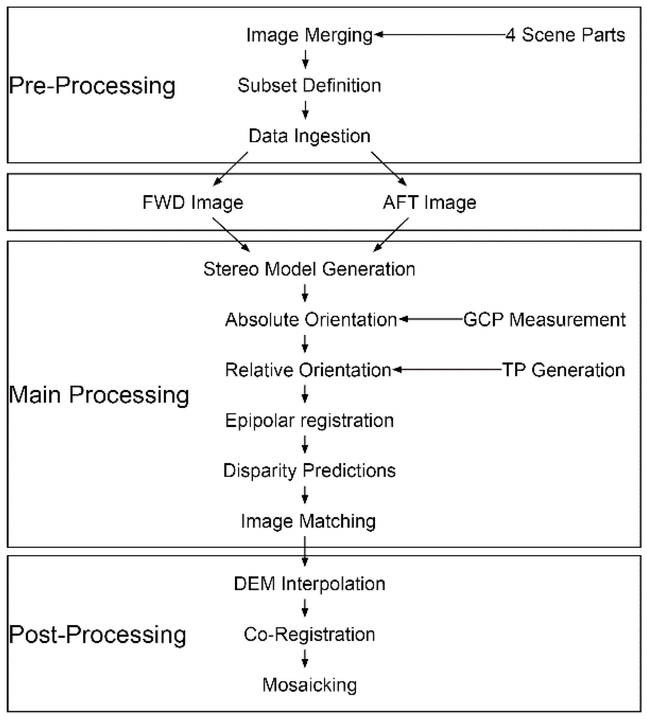
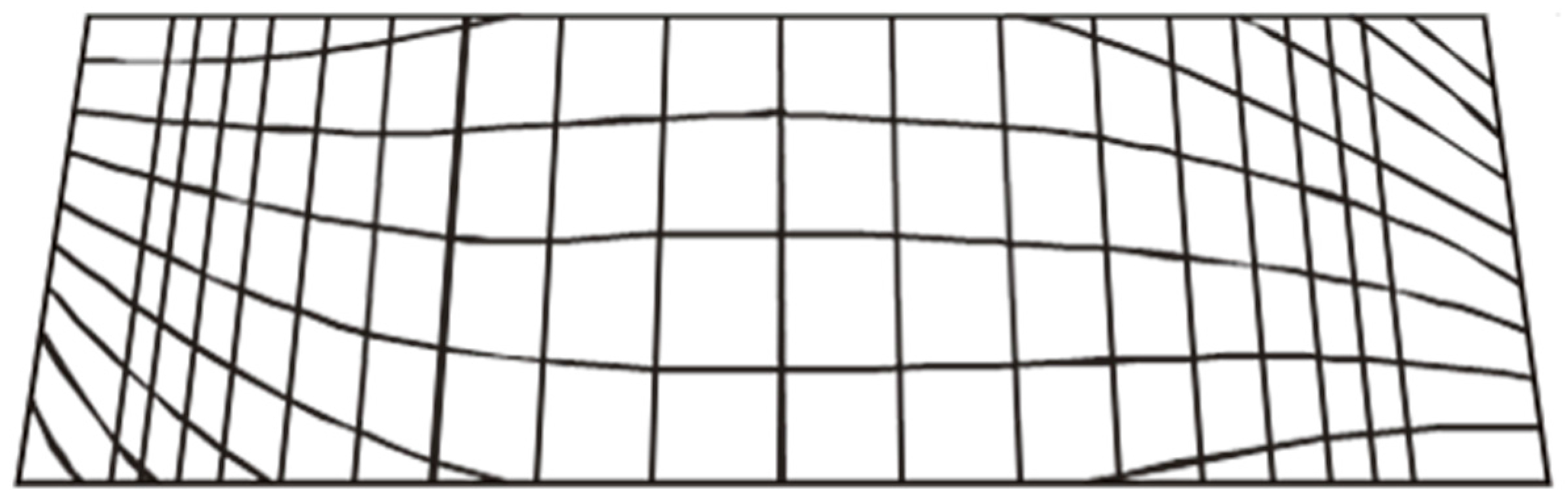
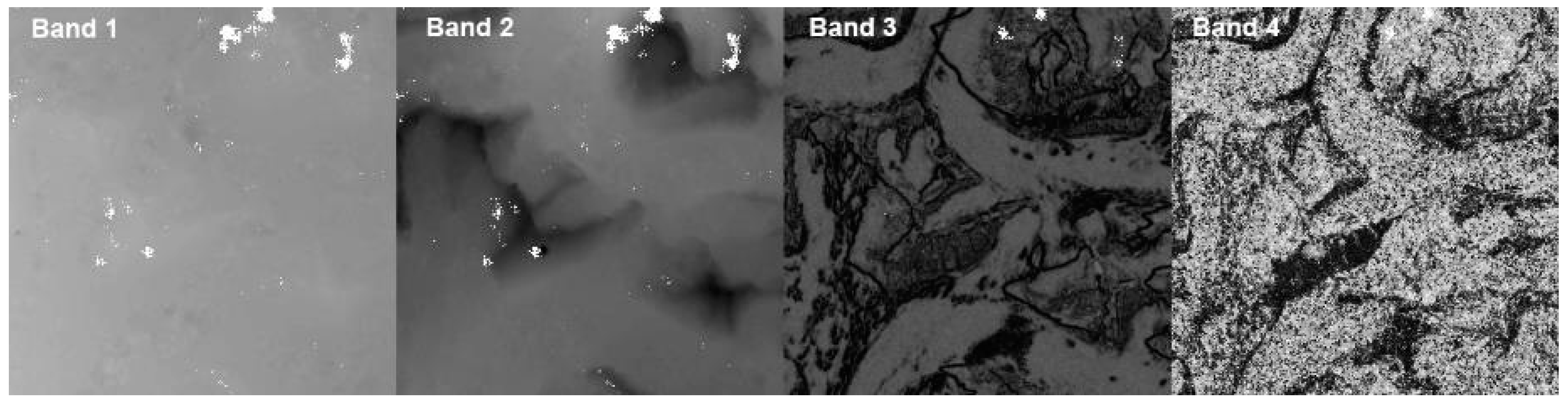
The results of the mass budgets show relatively low uncertainties according to the results of the selected method [42]. However, we found some problems with the Corona data in general. A first aspect is the scanner used for the digitalisation of the analogue images. If the image is not perfectly adjusted during scanning, it is nearly impossible to recreate the entire scene from the four provided subsets. Furthermore, we detected small differences in the scanner head velocities, resulting in an impossibility to apply an epipolar registration (R. Perko, K. Gutjahr, pers. comm., 21 April 2015). Galiatsatos [28] described these findings as well.

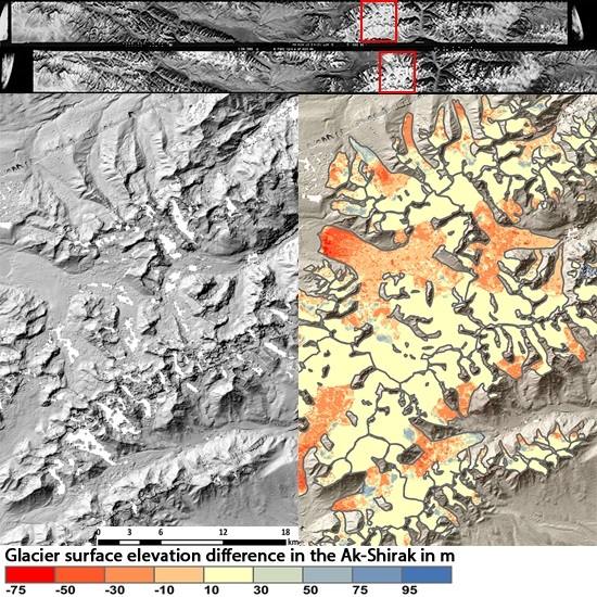
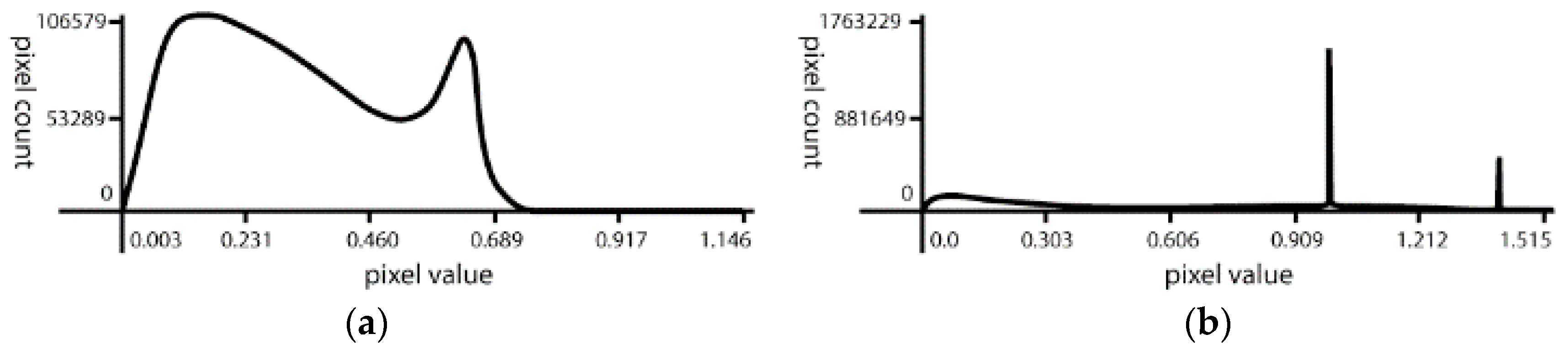
The second limitation is low image contrast in snow-covered or shadowed areas where matching failed and resulted in data gaps (~2.4% of the entire DTM; ~4% of glacierised terrain) and wrongly assigned pixels after DTM generation. This lowered the number of pixels for the uncertainty calculations and increased the number of pixels, which had to be interpolated, especially in the accumulation regions. We therefore compared our results to a second approach with an elevation-dependent filtering and an ordinary kriging interpolation without the threshold filter. For Bordu South Glacier, we found an unrealistic mass gain of 0.6 ± 0.3 m·w.e.a⁻¹ for the 1964 to 1973 period. The reason is clearly visible in the orthophoto where extremely low contrast results in wrongly assigned elevation values. The large glaciers showed only small differences, for example Dschamansu Glacier with −0.8 ± 0.4 instead of −0.6 ± 0.4 m·w.e.a⁻¹ (1964–1973) or Petrov with −0.7 ± 0.1 instead of −0.6 ± 0.1 m·w.e.a⁻¹ (1964–1980).

In comparison to previous work on Corona DTM generation in glacierised high mountain regions of smaller or equal 100 km² [21,22,23,24,46], we generated a DTM covering an area of ~4200 km² out of three stereo scenes, which is more than three times the size of the Ak-Shirak range. Besides the size of the DTM, it covers a high mountain region between 2500 m and 5200 m altitude. It consists of five single DTMs computed from six Corona scene subsets. The overlap of 9.7% impedes a perfect DTM mosaicking and is slightly visible in the final DTM. However, as the affected glacierised area is small (~12% of the glacierised area) and showing a median elevation difference of 9.5 m, there is a minor effect (±0.13 to ±0.07 m) on the mass budget accuracy calculations only. Another proof of the high quality of the generated DTM is the small amount of wrongly calculated surface elevation heights on stable terrain (Supplementary Materials Figure S1).

Apart from the uncertainty calculation approach of Gardelle et al. [42], we also took the approach of Höhle and Höhle [47] into account. The normalised median absolute deviation (NMAD) is a rather conservative approach also mentioned by Kronenberg et al. [26], which resulted in higher uncertainty values. For the sake of comparison, we did the entire uncertainty calculation for both approaches. This leads to uncertainty differences for Sary-Tor North Glacier of 6.1 m (1964–1980) with the approach of Gardelle et al. [42] compared to 8.3 m [47]. For Besimjannij Glacier the difference is slightly higher (3.4 to 9.4 m) for the same observation period. In the end, the uncertainties depict an estimate only and might be somewhere in between.

Furthermore, we used Landsat OLI and SRTM data as a basis for GCP measurements as there was no other reference data available. Both sources provide lower image resolution than the processed data, which might lead to non-linear transformations. As Landsat orthoimagery is processed based on SRTM data, the two sources should be correctly aligned, except SRTM data voids where other elevation data are used. To handle the issue of non-linear transformations, we checked the hillshade extract of the SRTM and the Landsat OLI data visually if they are aligned adequately (mountain ridges and summits in snow covered regions) and can confirm satisfying alignment. Additionally, we did as many co-registration iterations between the generated DTMs (KH-4A and KH-9 1980) and the KH-9 1973 DTM until we reached a horizontal accuracy of less than 1 px, which proofs a correct alignment and less geometric distortions.

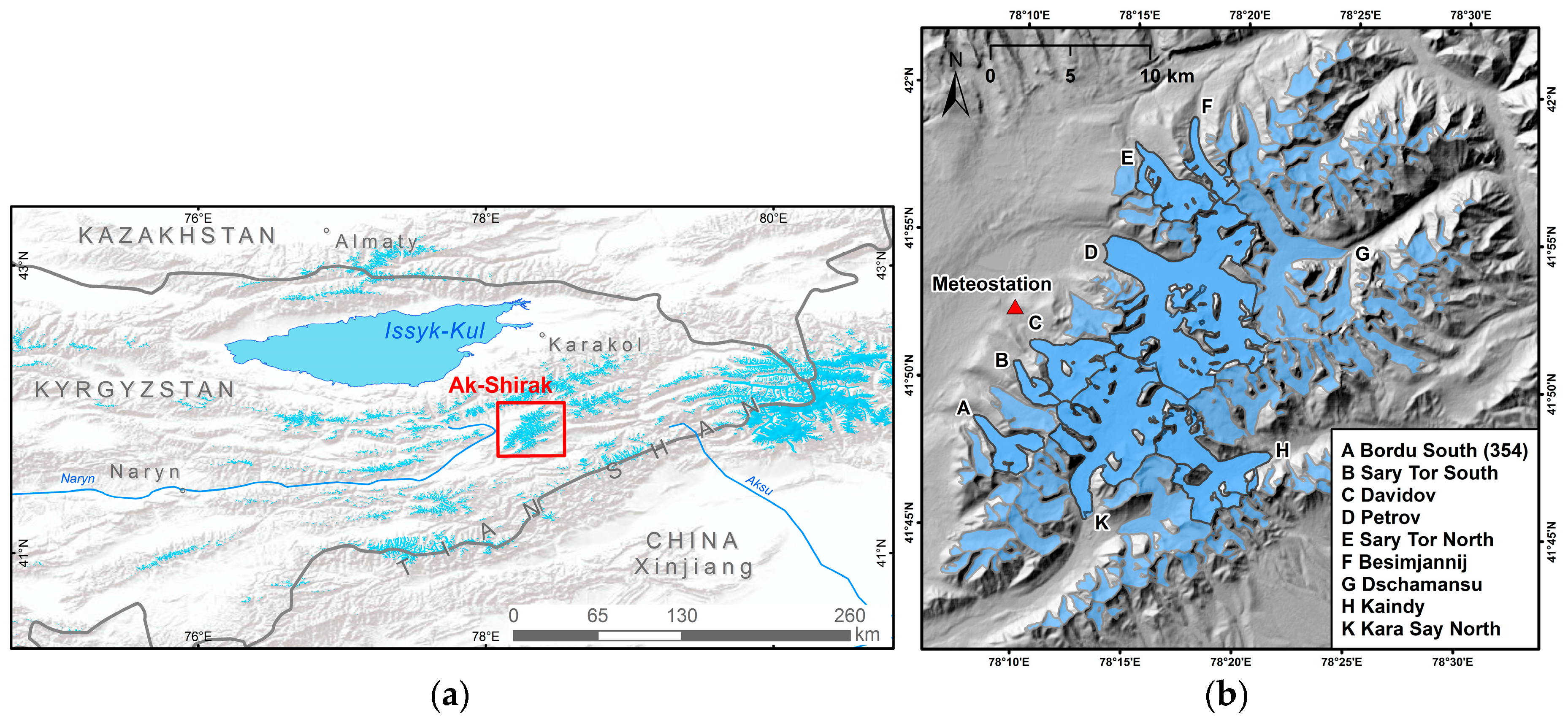
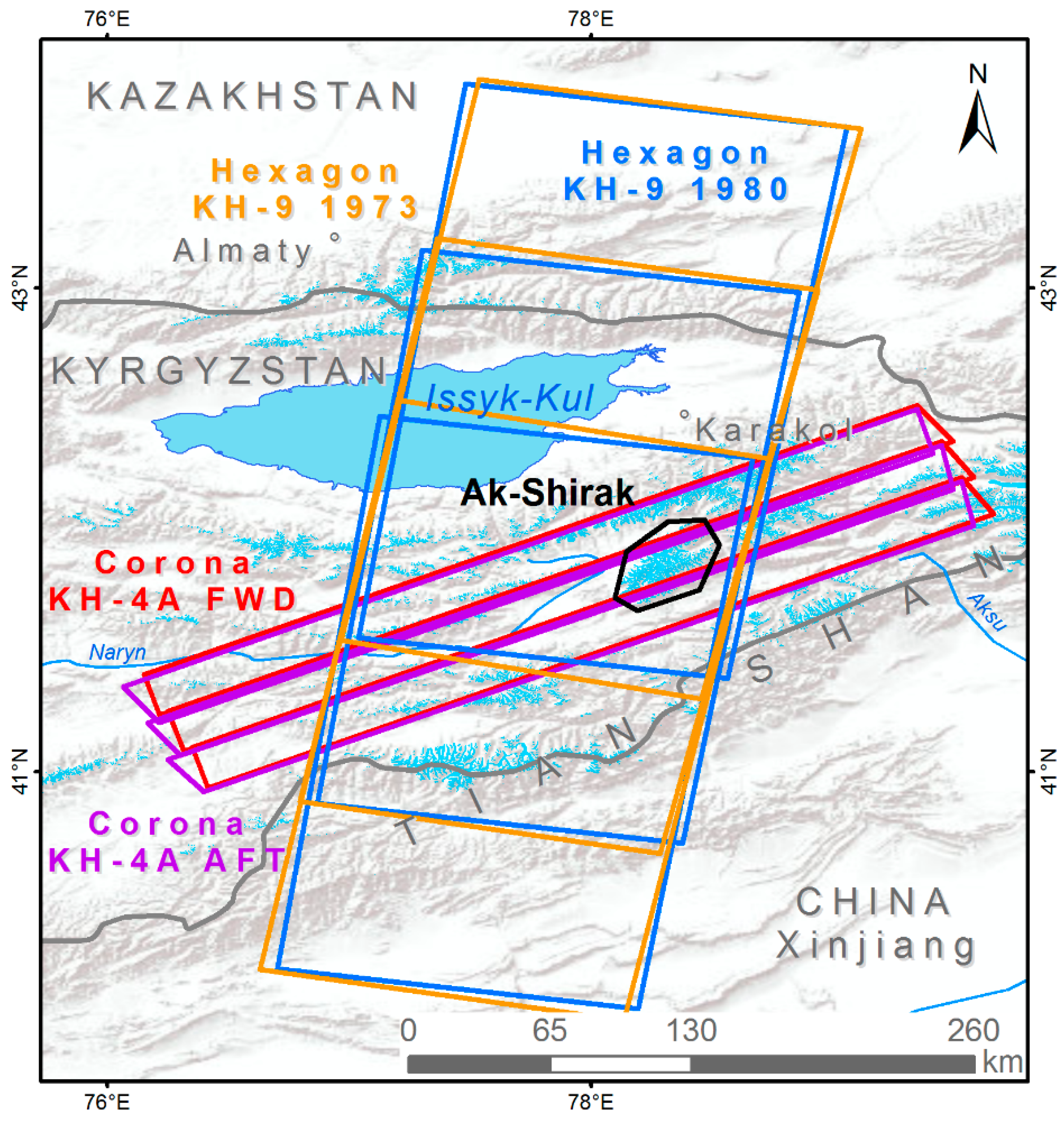
The Corona and Hexagon scenes are acquired in different seasons of the year, which might have an influence on the snow cover and thus the calculated surface elevation. These seasonal variations should be considered [48]. In this specific case, we did not apply any seasonal corrections because the Ak-Shirak is situated in an arid region (mean annual precipitation measured at Tian Shan station ~320 mm, elevation 3614 m a.s.l., Figure 1) with precipitation maximum in summer and very low precipitation [8] in winter. Additionally, the acquired scenes show no visible differences in snow cover (Supplementary Materials Figure S2) and thus the seasonal effect is within the estimated uncertainty.

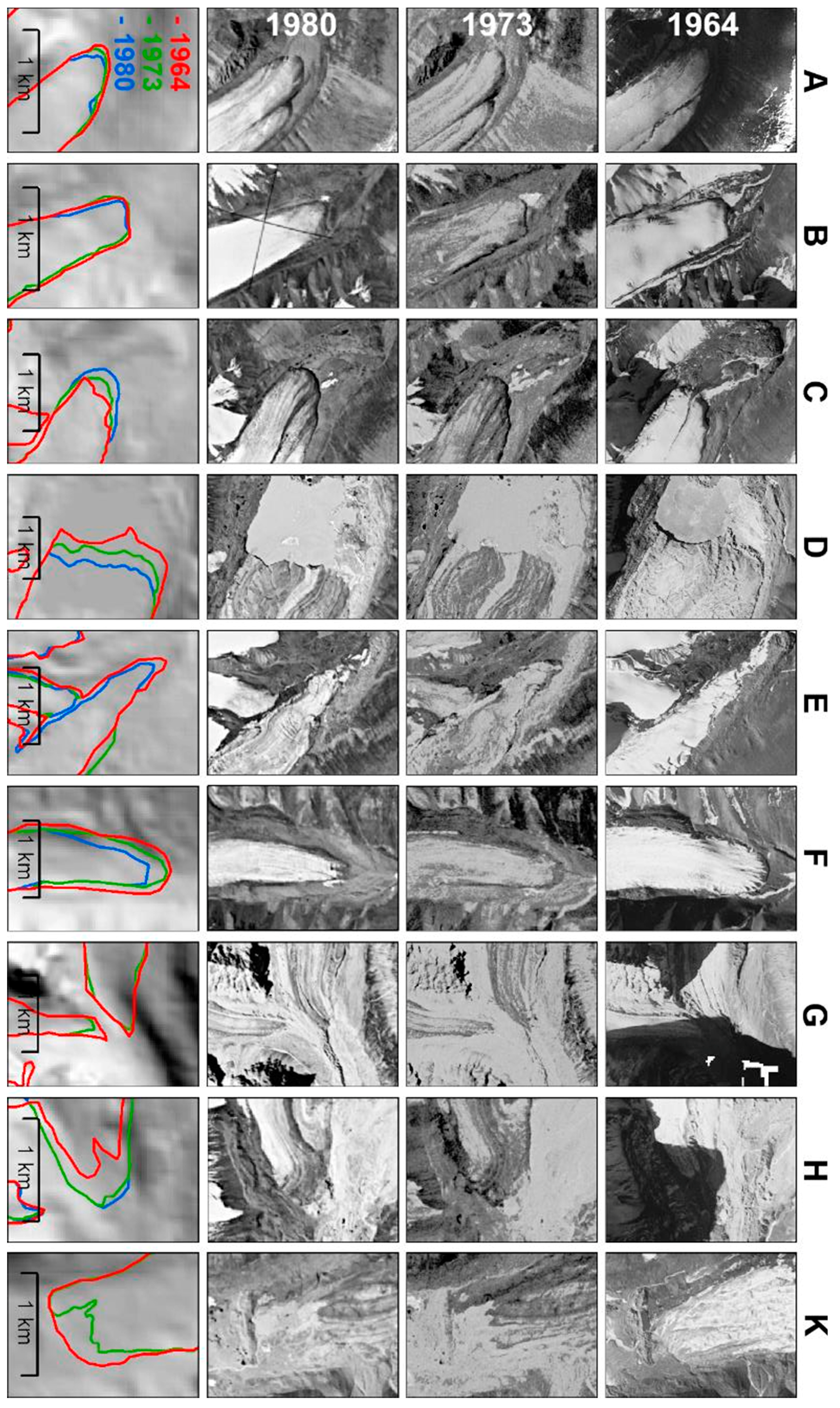
Besides data handling difficulties mentioned above, there is a high potential for the use of declassified Corona imagery for glacier research [20,21,22,23,24,46] but also on many other research fields like archaeology [16,17,49] or surficial mass movements [50]. The major advantage of our processing line is a true orthorectification of the highly-distorted Corona reconnaissance imagery resulting in higher precision in comparison to previous studies, which simplifies feature detection (e.g., for archaeology) and surface change detection. As displayed in Figure 8, the high resolution of the KH-4A and KH-9 images reflect in general far more details of glacier surface structures and landforms than more recent freely available data such as Landsat images. Moreover, glacier volume changes, glacier velocities [51] and speed up events can be detected by the huge number of scenes, which are available for the Central Asian mountain regions and could lead to unexpectedly dense multi-temporal time series with high spatial resolution.

4.2. Mass Budget

We found negative mass budgets for both analysed periods while the annual values for the period from 1964 to 1973 are comparable (−0.4 ± 0.2 m·w.e.a⁻¹) to the 1964–1980 period (−0.4 ± 0.1 m·w.e.a⁻¹). The negative values are generally in agreement with Aizen et al. [10] who analysed the period from 1943 to 1977 based on aerial photographs and found glacier surface elevation lowering rates of −0.24 ± 0.12 m·a⁻¹ equivalent to −0.20 ± 0.10 m·w.e.a⁻¹ with the ice density parameters assumed in our study. However, our values for the 1964–1980 period are more negative. Although we expected an increase in glacier mass loss for the entire observation period due to a slight temperature increase and precipitation decrease recorded by the nearby Tian Shan meteorological station [52] (for location see Figure 1), the trend does not lead to a significant increase of the mass loss. Pieczonka and Bolch [5] found similar negative mass budget rates of 0.51 ± 0.25 m·w.e.a⁻¹ for the period from 1975 to 1999. Gardner et al. [53] found mass loss of 0.49 ± 0.08 m·w.e.a⁻¹ between 2003 and 2009 for the entire Tien Shan; however, mass loss in the Central Tian Shan is lower compared to the outer ranges [3,53].

A glacier-specific analysis reflects a different situation with an increasing mass loss for the time after 2003. Kronenberg et al. [26] found mass changes for Bordu South Glacier (No. 354) of −0.43 ± 0.09 m·w.e.a⁻¹ from 2003 to 2012, which are higher than our calculated mass budgets from 1964–1980 (−0.3 ± 0.1 m·w.e.a⁻¹). All other individual glaciers show maximum mass loss rates of 0.9 ± 0.6 m·w.e.a⁻¹ until 1973 with a subsequent loss to 0.7 ± 0.2 m·w.e.a⁻¹ until 1980. Dschamansu Glacier with its terminus situated at 3660 m and an eastern aspect and displays the strongest absolute mass loss of 11.4 ± 3.9 m w.e. between 1964 and 1980. Regarding the observed length changes, Kara-Say North Glacier, on the other hand, showed a decelerating retreat rate. Besimjannij, Sary-Tor North and Petrov glaciers had the highest negative rates up to −33.5 ± 2 m·a⁻¹ whilst Besimjannij Glacier seemed to be in the retreat phase after a surge and Petrov Glacier calves in a large proglacial lake (Figure 8), both favouring terminus retreat [54]. The glaciers classified here as surge-type glaciers were also mentioned in other studies [6,7].

For Sary-Tor South Glacier, our mass budget rates of −0.3 ± 0.4 m·w.e.a⁻¹ between 1964 and 1980 agree with Kuzmichenok [55] and Petrakov et al. [56]. For the period from 1943 to 1977 they found values of −0.48 m·w.e.a⁻¹, respectively. Furthermore, the −0.3 ± 0.4 m·w.e.a⁻¹ found here for Sary-Tor South (1964–1980) are within the uncertainty range of mass budget measurements taken from 1985 to 1989 at the same glacier (−0.14 m·w.e.a⁻¹) [57].

Finally, we found out that glaciers in the Ak-Shirak massif showed significant mass loss since the 1960s accompanied by a glacier retreat on average. Particularly Petrov and Kara-Say North glaciers showed strong retreats up to 24.2 ± 2.6 m·a⁻¹ between 1964 and 1973 and corresponding elevation lowering rates.

5. Conclusions

In this study, we presented a new approach of processing declassified Corona imagery at a larger scale for the entire Ak-Shirak massif in the Central Tian Shan. Even if key processing steps still had been performed manually (GCP assignment), the importance of declassified KH-4 Corona and KH-9 Hexagon data is obvious, especially through its high resolution of ≤7.6 m. We thus see a great potential on the processing and evaluation of Corona data regarding two- and three-dimensional environmental changes that should be further exploited.

Glaciers in the Ak-Shirak lost −0.4 ± 0.2 m·w.e.a⁻¹ of mass between 1964 and 1973. Downwasting rates of the observed individual glaciers prove a clear negative trend before the early 1970s. Furthermore, we found negative mass budgets until 1980 as well. Petrov and Dschamansu glaciers, two of the largest glaciers in the mountain range, showed obvious mass loss rates up to 0.7 ± 0.2 m·w.e.a⁻¹ and glacier terminus retreats up to 923 ± 18 m (−57.7 ± 1.1 m·a⁻¹) in the 1964–1980 period. Additionally, four surge-type glaciers could be identified by our study considering the spatial pattern of the observed thickness changes in combination with the measured length changes surface structures.

References

1. Sorg, A.; Bolch, T.; Stoffel, M.; Solomina, O.; Beniston, M. Climate change impacts on glaciers and runoff in Tien Shan (Central Asia). Nat. Clim. Chang. 2012, 2, 725–731. [Google Scholar] [CrossRef]
2. Unger-Shayesteh, K.; Vorogushyn, S.; Farinotti, D.; Gafurov, A.; Duethmann, D.; Mandychev, A.; Merz, B. What do we know about past changes in the water cycle of Central Asian headwaters? A review. Glob. Planet. Chang. 2013, 110, 4–25. [Google Scholar] [CrossRef]
3. Farinotti, D.; Longuevergne, L.; Moholdt, G.; Duethmann, D.; Mölg, T.; Bolch, T.; Vorogushyn, S.; Güntner, A. Substantial glacier mass loss in the Tien Shan over the past 50 years. Nat. Geosci. 2015, 8, 716–722. [Google Scholar] [CrossRef]
4. Kriegel, D.; Mayer, C.; Hagg, W.; Vorogushyn, S.; Duethmann, D.; Gafurov, A.; Farinotti, D. Changes in glacierisation, climate and runoff in the second half of the 20th century in the Naryn basin, Central Asia. Glob. Planet. Chang. 2013, 110, 51–61. [Google Scholar] [CrossRef]
5. Pieczonka, T.; Bolch, T. Region-wide glacier mass budgets and area changes for the Central Tien Shan between ~1975 and 1999 using Hexagon KH-9 imagery. Glob. Planet. Chang. 2015, 128, 1–13. [Google Scholar] [CrossRef]
6. Dolgoushin, L.D.; Osipova, G.B. Glacier surges and the problem of their forecasting. IAHS Publ. 1975, 104, 292–304. [Google Scholar]
7. Mukherjee, K.; Bolch, T.; Goerlich, F.; Kutuzov, S.; Osmonov, A.; Pieczonka, T.; Shesterova, I. Surge-type glaciers in the Tien Shan (Central Asia). Arct. Antarct. Alp. Res. 2017, 49, 147–171. [Google Scholar] [CrossRef]
8. Ozmonov, A.; Bolch, T.; Xi, C.; Wei, J.; Kurban, A. Glaciers characteristics and changes in the Sary-Jaz River Basin (Central Tien Shan) 1990–2010 Remote Sensing Letters. Remote Sens. Lett. 2013, 4, 725–734. [Google Scholar] [CrossRef]
9. Koscielny-Bunde, E.; Bunde, A.; Havlin, S.; Roman, H.E.; Goldreich, Y.; Schellnhuber, H.J. Indication of a universal persistence law governing atmospheric variability. Phys. Rev. Lett. 1998, 81, 729. [Google Scholar] [CrossRef]
10. Aizen, V.B.; Kuzmichenok, V.A.; Surazakov, A.B.; Aizen, E.M. Glacier changes in the Tien Shan as determined from topographic and remotely sensed data. Glob. Planet. Chang. 2007, 56, 328–340. [Google Scholar] [CrossRef]
11. Kuzmichenok, V.A. Fluctuations in the condition of Davydov and Sary-Tor glaciers according to the topographic survey data. Mater. Glyaciol. Issled. 1988, 62, 193–198. (In Russian) [Google Scholar]
12. Maurer, J.M.; Rupper, S.B.; Schaefer, J.M. Quantifying ice loss in the eastern Himalayas since 1974 using declassified spy satellite imagery. Cryosphere 2016, 10, 2203. [Google Scholar] [CrossRef]
13. Bolch, T.; Pieczonka, T.; Mukherjee, K.; Shea, J. Brief Communications: Glaciers in the Hunza Catchment (Karakoram) have been almost in balance since the 1970s. Cryosphere 2017, 11. [Google Scholar] [CrossRef]
14. Pieczonka, T.; Bolch, T.; Junfeng, W.; Shiyin, L. Heterogeneous mass loss of glaciers in the Aksu-Tarim Catchment (Central Tien Shan) revealed by 1976 KH-9 Hexagon and 2009 SPOT-5 stereo imagery. Remote Sens. Environ. 2013, 130, 233–244. [Google Scholar] [CrossRef] [Green Version]
15. U.S. Geological Survey. Declassified Intelligence Satellite Photographs: U.S. Geological Survey Fact Sheet 2008–3054; U.S. Geological Survey: Reston, VA, USA, 2008.
16. Beck, A.; Philip, G.; Abdulkarim, M.; Donoghue, D. Evaluation of Corona and Ikonos high resolution satellite imagery for archaeological prospection in western Syria. Antiquity 2007, 81, 161–175. [Google Scholar] [CrossRef] [Green Version]
17. Altmaier, A.; Kany, C. Digital surface model generation from CORONA satellite images. ISPRS J. Photogram. Remote Sens. 2002, 56, 221–235. [Google Scholar] [CrossRef]
18. Schmidt, S.; Nüsser, M. Changes of high altitude glaciers from 1969 to 2010 in the trans-Himalayan Kang Yatze Massif, Ladakh, northwest India. Arct. Antarct. Alp. Res. 2012, 44, 107–121. [Google Scholar] [CrossRef]
19. Narama, C.; Kääb, A.; Duishonakunov, M.; Abdrakhmatov, K. Spatial variability of recent glacier area changes in the Tien Shan Mountains, Central Asia, using Corona (~1970), Landsat (~2000), and ALOS (~2007) satellite data. Glob. Planet. Chang. 2010, 71, 42–54. [Google Scholar] [CrossRef]
20. Bhambri, R.; Bolch, T.; Chaujar, R.K. Frontal recession of Gangotri Glacier, Garhwal Himalayas, from 1965 to 2006, measured through highresolution remote sensing data. Curr. Sci. 2012, 102, 489–494. [Google Scholar]
21. Bolch, T.; Buchroithner, M.; Pieczonka, T.; Kunert, A. Planimetric and volumetric glacier changes in the Khumbu Himal, Nepal, since 1962 using Corona, Landsat TM and ASTER data. J. Glaciol. 2008, 54, 592–600. [Google Scholar] [CrossRef]
22. Bolch, T.; Pieczonka, T.; Benn, D.I. Multi-decadal mass loss of glaciers in the Everest area (Nepal Himalaya) derived from stereo imagery. Cryosphere 2011, 5, 349–358. [Google Scholar] [CrossRef] [Green Version]
23. Bolch, T. Glacier area and mass changes since 1964 in the Ala Archa Valley, Kyrgyz Ala-Too, northern Tien Shan. Лёд и Снег (Ice and Snow) 2015, 1, 28–39. [Google Scholar] [CrossRef]
24. Lamsal, D.; Sawagaki, T.; Watanabe, T. Digital terrain modelling using Corona and ALOS PRISM data to investigate the distal part of Imja Glacier, Khumbu Himal, Nepal. J. Mount. Sci. 2011, 8, 390–402. [Google Scholar] [CrossRef]
25. Maurer, J.; Rupper, S. Tapping into the Hexagon spy imagery database: A new automated pipeline for geomorphic change detection. ISPRS J. Photogramm. Remote Sens. 2015, 108, 113–127. [Google Scholar] [CrossRef]
26. Kronenberg, M.; Brandun, M.; Hoelzle, M.; Huss, M.; Farinotti, D.; Azisov, E.; Usubaliev, R.; Gafurov, A.; Petrakov, D.; Kääb, A. Mass-balance reconstruction for Glacier No. 354, Tien Shan, from 2003 to 2014. Ann. Glaciol. 2015, 57, 92–102. [Google Scholar] [CrossRef]
27. Dashora, A.; Lohani, B.; Malik, J.N. A repository of earth resource information-CORONA satellite programme. Curr. Sci. 2007, 92, 926–932. [Google Scholar]
28. Galiatsatos, N. The shift from film to digital product: Focus on CORONA imagery. Photogramm. Fernerkund. Geoinf. 2009, 2009, 251–260. [Google Scholar] [CrossRef] [PubMed]
29. Kaufmann, V.; Sulzer, W. Über die Nutzungsmöglichkeit hochauflösender amerikanischer Spionage-Satellitenbilder (1960–1972). Vermess. Geoinf. 1997, 3, 97. [Google Scholar]
30. Schneider, T.; Jacobsen, K.; Seitz, R.; Förster, B. Remote sensing based parameter extraction for erosion control purposes in the Loess plateau of China. In Proceedings of ISPRS/EARSeL Joint Workshop on High-Resolution Mapping from Space, Hannover, Germany, 19–21 September 2001.
31. Burnett, M. Hexagon (KH-9) Mapping Program and Evolution; National Reconnaissance Office: Chantilly, Virginia, 2012.
32. Surazakov, A.; Aizen, V. Positional accuracy evaluation of declassified Hexagon KH-9 mapping camera imagery. Photogramm. Eng. Remote Sens. 2010, 76, 603–608. [Google Scholar] [CrossRef]
33. Rabus, B.; Eineder, M.; Roth, A.; Bamler, R. The shuttle radar topography mission—A new class of digital elevation models acquired by spaceborne radar. ISPRS J. Photogramm. Remote Sens. 2003, 57, 241–262. [Google Scholar] [CrossRef]
34. Berthier, E.; Arnaud, Y.; Vincent, C.; Remy, F. Biases of SRTM in high-mountain areas: Implications for the monitoring of glacier volume changes. Geophys. Res. Lett. 2006, 33. [Google Scholar] [CrossRef]
35. EarthExplorer. Available online: http://earthexplorer.usgs.gov/ (accessed on 21 March 2016).
36. Förstner, W.; Gülch, E. A fast operator for detection and precise location of distinct points, corners and centres of circular features. In Proceedings of the ISPRS Intercommission Conference on Fast Processing of Photogrammetric Data, Interlaken, Switzerland, 2–4 June 1987; pp. 281–305.
37. Pieczonka, T.; Bolch, T.; Buchroithner, M. Generation and evaluation of multitemporal digital terrain models of the Mt. Everest area from different optical sensors. ISPRS J. Photogramm. Remote Sens. 2011, 66, 927–940. [Google Scholar] [CrossRef]
38. Nuth, C.; Kääb, A. Co-registration and bias corrections of satellite elevation data sets for quantifying glacier thickness change. Cryosphere 2011, 5, 271. [Google Scholar] [CrossRef]
39. Koblet, T.; Gärtner-Roer, I.; Zemp, M.; Jansson, P.; Thee, P.; Haeberli, W.; Holmlund, P. Reanalysis of multi-temporal aerial images of Storglaciären, Sweden (1959–99)–Part 1: Determination of length, area, and volume changes. Cryosphere 2010, 4, 333–343. [Google Scholar] [CrossRef] [Green Version]
40. Huss, M.; Jouvet, G.; Farinotti, D.; Bauder, A. Future high-mountain hydrology: A new parameterization of glacier retreat. Hydrol. Earth Syst. Sci. 2010, 14, 815–829. [Google Scholar] [CrossRef]
41. Sapiano, J.J.; Harrison, W.T.; Echelmeyer, K.A. Elevation, volume and terminus changes of nine glaciers in North America. J. Glaciol. 1998, 44, 119–135. [Google Scholar] [CrossRef]
42. Gardelle, J.; Berthier, E.; Arnaud, Y.; Kääb, A. Region-wide glacier mass balances over the Pamir-Karakoram-Himalaya during 1999–2011. Cryosphere 2013, 7, 1885–1886. [Google Scholar] [CrossRef] [Green Version]
43. Huss, M. Density assumptions for converting geodetic glacier volume change to mass change. Cryosphere 2013, 7, 877–887. [Google Scholar] [CrossRef]
44. Bolch, T.; Menounos, B.; Wheate, R. Landsat-based inventory of glaciers in western Canada, 1985–2005. Remote Sens. Environ. 2010, 114, 127–137. [Google Scholar] [CrossRef]
45. Hall, D.K.; Bayr, K.J.; Schöner, W.; Bindschadler, R.A.; Chien, J.Y. Consideration of the errors inherent in mapping historical glacier positions in Austria from the ground and space (1893–2001). Remote Sens. Environ. 2003, 86, 566–577. [Google Scholar] [CrossRef]
46. Pieczonka, T.; Bolch, T.; Buchroithner, M. Volumetric glacier changes in the Khumbu Himal since 1962 using space imagery. Grazer Schriften der Geographie und Raumforschung 2010, 45, 295–302. [Google Scholar]
47. Höhle, J.; Höhle, M. Accuracy assessment of digital elevation models by means of robust statistical methods. ISPRS J. Photogramm. Remote Sens. 2009, 64, 398–406. [Google Scholar] [CrossRef]
48. Magnússon, E.; Muñoz-Cobo Belart, J.; Pálsson, F.; Ágústsson, H.; Crochet, P. Geodetic mass balance record with rigorous uncertainty estimates deduced from aerial photographs and lidar data—Case study from Drangajökull ice cap, NW Iceland. Cryosphere 2016, 10, 159–177. [Google Scholar] [CrossRef]
49. Goossens, R.; De Wulf, A.; Bourgeois, J.; Gheyle, W.; Willems, T. Satellite imagery and archaeology: The example of CORONA in the Altai Mountains. J. Archaeol. Sci. 2006, 33, 745–755. [Google Scholar] [CrossRef]
50. Meszaros, M.; Szatmari, J.; Tobal, Z.; Mucsi, L. Extraction of digital surface models from Corona satellite stereo images. J. Environ. Geogr. 2008, 1, 5–10. [Google Scholar]
51. Sorg, A.; Kääb, A.; Roesch, A.; Bigler, C.; Stoffel, M. Contrasting responses of Central Asian rock glaciers to global warming. Sci. Rep. 2015, 5, 8228. [Google Scholar] [CrossRef]
52. Khromova, T.E.; Dyurgerov, M.B.; Barry, R.G. Late-twentieth century changes in glacier extent in the Ak-shirak Range, Central Asia, determined from historical data and ASTER imagery. Geophys. Res. Lett. 2003, 30. [Google Scholar] [CrossRef]
53. Gardner, A.S.; Moholdt, G.; Cogley, J.G.; Wouters, B.; Arendt, A.A.; Wahr, J.; Berthier, E.; Hock, R.; Pfeffer, W.T.; Kaser, G.; et al. A reconciled estimate of glacier contributions to sea level rise: 2003 to 2009. Science 2013, 340, 852–857. [Google Scholar] [CrossRef] [PubMed] [Green Version]
54. Engel, Z.; Sobr, M.; Yerokhin, S.A. Changes of Petrov glacier and its proglacial lake in the Akshiirak massif, central Tien Shan, since 1977. J. Glaciol. 2012, 58, 388–398. [Google Scholar] [CrossRef]
55. Kuzmichenok, V.A. Statistical studies of the geometry of the valley glaciers of Kyrgyzstan. Mater. Glyaciol. Issled. 2006, 12, 80–86. (In Russian) [Google Scholar]
56. Petrakov, D.A.; Lavrientiev, I.I.; Kovalenko, N.V.; Usubaliev, R.A. Snow Cover and Glaciers Ice Thickness, Volume and Current Changes of the Sary-Tor Glacier Area (Ak-Shyirak Massif, Inner Tian Shan). Earth’s Cryosphere 2014, 18, 83–91. [Google Scholar]
57. World Glacier Monitoring Service (WGMS). Global Glacier Change Bulletin No. 1 (2012–2013). ICSU(WDS)/IUGG(IACS)/UNEP/UNESCO WMO; Zemp, M., Gärtner-Roer, I., Nussbaumer, S.U., Hüsler, F., Machguth, H., Mölg, N., Paul, F., Hoelzle, M., Eds.; World Glacier Monitoring Service: Zurich, Switzerland, 2015; p. 230. [Google Scholar]
Figure 1. Location of the study area within the Tian Shan (a); the glacierised Ak-Shirak massif showing the 1964 glacier extent. Investigated single glaciers are labelled with capital letters (b).
Remotesensing 09 00275 g001
Figure 2. Corona image distortion model (adapted from Schneider et al. [30]).
Remotesensing 09 00275 g002
Figure 3. Corona and Hexagon scene coverage of the study area.
Remotesensing 09 00275 g003
Figure 4. Corona DTM generation workflow. FWD, forward image; AFT, backward image.
Remotesensing 09 00275 g004
Figure 5. Small disparity map extract. Band 1: disparities in column direction; Band 2: disparities in line direction; Band 3: feature distances; Band 4: backmatching distances.
Remotesensing 09 00275 g005
Figure 6. Feature distances (a); and backmatching distances (b) of the disparity raster.
Remotesensing 09 00275 g006
Figure 7. Glacier surface elevation differences for the entire Ak-Shirak range for the 1964–1973 and 1973–1980 periods.
Remotesensing 09 00275 g007
Figure 8. Glacier tongue changes of individual glaciers on Corona KH-4A (1964), Hexagon KH-9 (1973 and 1980): (A) Bordu South (354); (B) Sary-Tor South; (C) Davidov; (D) Petrov; (E) Sary-Tor North; (F) Besimjannij; (G) Dschamansu; (H) Kaindy; and (K) Kara-Say North.
Remotesensing 09 00275 g008