
A SAR-Based Index for Landscape Changes in African Savannas


Institute for Geography, University of Tübingen, Rümelinstraße 19-23, 72070 Tübingen, Germany
*
Author to whom correspondence should be addressed.
Remote Sens. 2017, 9(4), 359; https://doi.org/10.3390/rs9040359
Submission received: 24 March 2017
/
Revised: 5 April 2017
/
Accepted: 9 April 2017
/
Published: 11 April 2017
(This article belongs to the Special Issue Advances in SAR: Sensors, Methodologies, and Applications)
Abstract
:Change detection is one of the main applications in earth observation but currently there are only a few approaches based on radar imagery. Available techniques strongly focus on optical data. These techniques are often limited to static analyses of image pairs and are frequently lacking results which address the requirements of the user. Some of these shortcomings include integration of user’s expertise, transparency of methods, and communication of results in a comprehensive understandable way. This study introduces an index describing changes in the savanna ecosystem around the refugee camp Djabal, Eastern Chad, based on a time-series of ALOS PALSAR data between 2007 and 2017. Texture based land-use/land cover classifications are transferred to values of natural resources which include comprehensive pertinent expert knowledge about the contributions of the classes to environmental integrity and human security. Changes between the images are analyzed, within grid cells of one kilometer diameter, according to changes of natural resources and the variability of these changes. Our results show the highest resource availability for the year of 2008 but no general decline in natural resources. Largest loss of resources occurred between 2010 and 2011 but regeneration could be observed in the following years. Neither the settlements nor the wadi areas of high ecologic importance underwent significant changes during the last decade.
1. Introduction
Detecting and understanding processes at the earth’s surface are among the key tasks of spaceborne remote sensing. Thousands of images stored in archives allow for the analysis of dense time-series of nearly every region of the earth. In particular is the Landsat continuity mission, delivering valuable data since the 1970s, which provides an excellent foundation of long-term observations [1,2]. Their potential for the mapping of land-use and land cover (LULC) has been demonstrated in numerous studies which exploit the temporal variability of the image information in different methodological frameworks [3,4,5,6,7,8,9,10]. Among others, Song et al. portray the problems regarding atmospheric disturbances in the data and raise the question to what extent these applications are affected by cloud cover [11]. Of primary concern is large-scaled classification of LULC often being constrained by cloud cover. According to the US Department of Energy, about 52% of global land surfaces are covered by clouds on average [12]. In particular, regions within the intertropical convergence zone (ITC) are highly affected by seasonal or full-year cloud coverage [13,14,15] which hinders proper analysis of LULC based on series of optical satellite imagery [16,17,18].
To overcome this dependency upon favorable atmospheric conditions, satellites with synthetic aperture radar (SAR), operating at wavelengths which can penetrate cloud cover, are employed. Their reliability in acquiring usable imagery is one of the main reasons to utilize them in LULC applications. Accordingly, the long-term missions of ERS-1/2 [19] and RADARSAT-1/2 [20], plus the relatively recent Sentinel-1 constellation [21] which was launched in 2014, show high potential for the investigation of changes in land cover over decades. They also serve well as complementary sources when operating at the same wavelength [22,23].
The use of SAR imagery has proven effective for LULC classification in many cases. Early studies mostly applied knowledge-based methods on SAR backscatter in order to separate different classes of land cover [24,25,26]. In fact, the first article published in Remote Sensing of Environment, back in 1969, was an interpretation key for SAR backscatter at the landscape level [27]. These studies require detailed a-priori knowledge about the study area but offer a high degree of control to the user. Additional features were used to further increase the classification quality in later approaches, mainly interferometric parameters such as coherence [28,29,30], but also textural information within the intensity values at different levels [31,32,33]. Besides these technological advances, new methods of supervised classification were developed to assign classes based on sample data. These were required because, in contrast to optical image information, SAR parameters are not necessarily of consistent units and value ranges. Among the most popular methods are Bayesian classifiers [34,35,36], neural networks [37,38,39] and random forest classifiers [40,41,42]. These developments targeting LULC classifications were complemented by progress in SAR polarimetry. Deeper knowledge of the backscattering behavior of surfaces and decompositions into different scattering mechanisms additionally increased the quality of analyses related to land cover [43,44,45,46].
Utilizing SAR imagery in a multi-temporal context to monitor changes in land-use or land cover requires particular attention because of the characteristics of image acquisition and signal propagation. While the very identification of areas of change is scientifically well-proven and widely-used [47,48,49], quantitative and long-term monitoring of distinct classes requires accurate calibration and a robust handling of speckle [50,51].
Studies investigating landscape sensitivity, the severity of disturbances and human impact based on SAR data are rare: Townsend and Foster proposed a statistical indicator for the intensity of flooding for the Roanoke River floodplain (United States) based on eleven RADARSAT-1 scenes acquired over a period of seventeen months [52]. They used the distinctive signature of water in SAR images expressed in usually very low backscatter values. They achieved overall model accuracies of 87.8%, however they only looked at two classes (flooded and non-flooded). Beisl et al. followed a similar approach for the estimation of landscape sensitivity towards floods based on two JERS-1 mosaics in Western Arizona [53]. Their study targeted four LULC classes and five levels of flood hazards but only compared two images (pre- and post-flooding).
Hoffmann et al. derived forest fire damage in East Kalimantan, Indonesia, based on 56 scenes of ERS-2 from 1997 [54]. They discriminated three different classes of burn severity and additionally derived a LULC classification. This study is one of the few making full use of large SAR archives for the assessment of impacts of disturbances on landscapes.
As well, human impacts upon forest systems deforestation of the Amazon rainforests is of special interest in remote sensing studies. Saatchi et al. made use of the polarimetric covariance between channels of SIR-C [55], comparing an intra-annual pair of images—interferometric signatures and coherence [56]. L-band data have been found to be of special importance due to its pronounced interaction with vegetation volumes such as canopy structures [57,58,59]. Most of the studies, however, do not make use of large sets of SAR images provided by the JAXA archives.
For the African continent, Mitchard et al. have found a robust relationship for the estimation of biomass changes in savanna ecosystems [60,61]. They derived change maps based on 7 biomass classes for an image pair from 1997 (JERS-1) and 2007 (ALOS PALSAR).
Shen et al. used polarimetric RADARSAT-2 data to derive landscape metrics from eight LULC classes in the Nanjishan Wetland Nature Reserve, PR China [62]. Although this approach aims at a deeper understanding of the classified landscape it doesn’t make allowance to investigate temporal changes.
Based on the prior developments and findings we identified the following research deficits. While indices of spatial change based on optical data are numerous, there is almost no SAR-based methodology for long-term analysis of landscape developments at a class level. Pixel-based approaches developed for optical data are not applicable for SAR data as they do not allow for smaller misclassifications or isolated pixels arising from speckle effects. Additionally, most studies strongly focus on a stepwise comparison of image pairs without considering the total variation along the full time-series [63]. This is especially a problem in landscapes with high dynamics due to wild-fires, land degradation, vegetation encroachment or strong human impact. For those situations, distinct indices have to be developed, especially when dealing with SAR or very high resolution (VHR) optical data [64]. Other indices are highly elaborate but hard to read for people from outside the field of research. Accordingly, Walker and Peters argue that findings of multi-temporal remote sensing products are often complicated to read or even misleading and susceptible to making false conclusions [65].
In order to perform long-term analyses of landscape change independently from cloud cover, a robust and transparent approach based on radar data has to be developed. As a result, an integrative index should explain both the location and intensity of changes, as well as their implications for environmental integrity and human well-being. This index must be reproducible and adjustable to different needs of the users according to the significance of the targeted classes. Still, it has to be easy to interpret for anyone, especially because stakeholders and decision-makers are often not familiar with or interested in the technical background [66,67,68].
In this paper, we propose an approach challenging these requirements. For this purpose, we investigate landscape changes in a savannah ecosystem in Eastern Chad. As it is located at the southern border of the Sahel, desertification, impacts of climate change, and limited resources are of main concern [69,70]. These types of savannas are observed to show significant changes regarding vegetation persistence during the last two decades, both positive and negative [71]. The study is used to answer the following questions: How, where, and how much did the semi-arid landscape change during the last ten years? Can an overall decrease of natural resources, such as the availability of fire wood, be observed and to what extent? Do the LULC types show different developments regarding dynamics and variability? Can land degradation be observed in the direct surroundings of the settlements as an indicator of human impact? And finally, can these aspects be visualized in an output map which is easy to read and still includes the severity of changes during the entire period investigated?
2. Materials and Methods
2.1. Study Area
The study area is located in the center of the Sila region of Eastern Chad (Figure 1, upper right map). It hosts a total population of about 470,000 inhabitants, resulting in a moderately low population density of 12.5 inhabitants per square kilometer [72]. It includes the town of Goz Beïda and the refugee camp of Djabal which was opened to Sudanese refugees in 2004 as a consequence of the large influx of people seeking shelter from the Darfur crisis [73]. Djabal is one of numerous refugee settlements (both temporary and permanent) along the 500 km long Sudanese border within Chad’s territory which were established for people fleeing from civil war and environmental degradation [74,75].
The region lies at the southern border of the Sahel and is regularly affected by droughts [76] but receives more than 600 mm of annual precipitation on average, allowing for small-scaled agricultural use [77]. A decrease of summer rains and an increase of temperatures by 0.8° Celsius for the past 25 years have been reported, leading to both stronger dependency on crop yields and higher pressure on usable land [78]. Precipitation is mainly limited to the rainy season between June and September while the rest of the year is considered as highly arid. Climate can therefore be described as BSh (Hot semi-arid climate), referring to the Köppen-Geiger scheme.
The area is dominated by Precambrian bedrock and Tertiary sediments as it lies at the transition between the geological Sud province and the Nubian Shield within the Chad Basin [79]. Both camp Djabal and Goz Beïda are located at around 575 m above sea level but they are framed by the Hadjer Arkop massif in the south and northwest reaching up to 900 m [80]. Due to its location at the transition from desert to savannas most of the study area is covered by edaphic grassland, rupicolous shrubs, and scattered dry forest. Generally, tree cover is sparse in this area and mainly consists of single deciduous trees of the Combretaceae family [81]. The ridges of the Hadjer Arkop massif are sparsely covered by various Boswellia trees and shrubs [82]. Wadi Aouada, ranging from West to North across the study area, is accompanied by smaller semi-deciduous riparian forests (Figure 1, main map). Agricultural use of this land lies at around 30% and mainly concentrates around the few settlements. It is composed of small-scaled semi-permanent cultivation and bush fallow.
Goz Beïda lies along an important transport axis of Eastern Chad which connects the large cities of the North (Fada) with the ones in the South (Sarh). A Dutch military base (Ciara) under the mandate of the European Union was temporarily established between 2008 and 2009 as an additional peace force in the region [83]. Today, only the Goz Beïda airport remains at this location.
2.2. Data and Pre-Processing
2.2.1. Satellite Imagery
As the investigated ecosystem shows strong seasonal dynamics, the data to be used should be selected carefully. Therefore, all investigated data were acquired during the dry season which extends from November until March where rainfall below 5 mm is expected. These conditions are favorable because SAR backscatter strongly varies with changing soil moisture. This could cause temporally misleading signatures during the rainy season, e.g., high values at smooth and non-vegetated bare soil. Additionally, overall vegetation dynamics are smaller during the dry season which increases the inter-annual comparability of the images despite smaller temporal differences.
Table 1 lists all satellite images used in this study. Considering its temporal coverage, wavelength, and high spatial resolution, ALOS PALSAR has been chosen as a main input. Landsat data was additionally used for the collection of reference data. For each year analyzed, a pair of ALOS and Landsat imagery has been found with a temporal difference Δt between 0 and 30 days. There is a gap of observation between 2012 and 2015 because the ALOS PALSAR archive only features data between 2006 and 2011 and ALOS-2 (Daichi) was launched in May 2014. Landsat ETM+ data experienced a failure of its Scan Line Corrector mechanism in May 2003 causing striped gaps in the data (SLC-off) [84]. However, our study area lies in the center of the scene where this effect is minimal, since 2015 data from Landsat 8 (OLI/TIRS) could be used instead.
2.2.2. Pre-Processing and Collection of Samples
ALOS data was obtained as Level 1.1 products in Slant Range Complex format [85,86]. Pre-processing included radiometric calibration to radar brightness (Beta Naught, β° [87]), multi-looking (n = 2), terrain flattening to normalize radiometric effects caused by different incidence angles (Flattened Gamma Naught, γ° [88]) and Range-Doppler terrain correction to adjust topographic distortions using a digital elevation model (1 Arc-Second SRTM) [89]. All rasters were resampled to a common ground resolution of 30 m. No speckle filtering was applied in order to conserve image texture as accuracies of classifications based on SAR texture alone are reported to decrease when speckle was removed [90,91].
In order to derive additional information layers we derived image textures based on the concept of Grey-Level Co-Occurrence Matrix (GLCM) [92] consisting of Cluster Prominence, Cluster Shade, Correlation, Difference Of Entropies, Difference Of Variances, Energy, Entropy, Grey-Level Nonuniformity, HT10, Haralick Correlation, High Grey-Level Run Emphasis, IC1, IC2, Inertia, Inverse Difference Moment, Long Run Low Grey-Level Emphasis, Low Grey-Level Run Emphasis, Mean, Run Length Non-uniformity, Run Percentage, Short Run High Grey-Level Emphasis, Short Run Low Grey-Level Emphasis, Sum Entropy, Sum Variance, and Variance. Each of these 25 textures was calculated for kernels of 3, 9, and 15 pixels in order to extract patterns emerging at different spatial scales, leading to a total of 75 SAR texture layers per analyzed year.
Landsat data was obtained as Level-1T (terrain corrected) products. All rasters were radiometrically corrected by applying conversion top of atmosphere (TOA) reflectance and dark object subtraction (DOS) [93,94].
Six LULC classes were defined for the analysis: (1) urban areas, (2) bare soil, (3) bare rock, (4) grassland, (5) shrubland, and (6) forest. We did not include water as a separate class since the study area does not feature any permanent water bodies and the few remaining temporary flooded areas are covered by the forests of Wadi Aouada.
Each class is represented by training areas which were automatically derived from the Landsat scenes. We utilized indices and threshold values from several studies to define areas which characterize the corresponding class to a best possible degree in each scene. These are listed in Table 2. The selection of training samples underlies two steps. First, representative areas for every class are derived in each year observed (see Table 1). Areas which are assigned to the same class throughout all scenes were then considered as stable over time and transparent according to the corresponding LULC. For example, a Normalized Difference Vegetation Index (NDVI) value greater than 0.2 is reported as high for the dry season in Sudanian savanna as found in the study area [95]. If a pixel fulfills this criterion throughout all images it was considered as forest. Information from near infrared (NIR) and short wave infrared (SWIR) bands was used for criteria of the classes grassland and shrubland but also for thresholds for the abiotic surfaces of bare rock and soil. As reference for urban areas, the extent of camp Djabal in the year 2007 was digitized from the Landsat image. These areas are observed to be stable over time as the camp reached a stable phase.
To prevent misclassifications, we removed areas smaller than 500,000 m2 from the identified sample areas. Recognizing the these kinds of savanna ecosystems are highly affected by wildfires [96], we calculated the Normalized Burn Ratio (NBR [97]) for all years and scenes. This characterizes burnt areas which were excluded from the identification of sample areas because they no longer reveal which land cover was present before the fire. Furthermore, clouded areas were excluded throughout all scenes.
In a second step, a number of 1600 random points was generated within the remaining areas as sample locations for the SAR classification (see Section 2.3). This technique guarantees that the sample points were chosen both stratified and random while partially respecting the spatial occurrence of each class within the study area. Table 2 lists the criteria used for their identification of the sample areas and the final number of samples per class.
Figure 2 shows the remaining areas which were used for the stratified random sampling. It shows the result of the criteria given in Table 2 which helped to identify stable LULC areas over the investigated period. Clearly visible are camp Djabal in the middle, surrounded by mostly bare soil resulting from less vegetation cover and agricultural use, the bare rocks of Hadjer Arkop and the denser forests of Wadi Aouada in the Northwest. As indicated in Figure 1 grassland and shrubland cover the wide plains in the North and East.
2.3. Image Classification
Image classification was performed for each SAR image in Table 1 in order to analyze the temporal developments in the study area. However, as a huge number of SAR textures are used covering many different value ranges in various units, traditional classifiers for pixel-based approaches—such as k-means clustering [100] or Maximum Likelihood estimation [101]—are not suitable. We therefore chose a Random Forest classifier (RF [102]) for our study. It is based on the concept of classification and regression trees (CARTs [103]) and repeatedly uses random subsets of the training data for the modeling of target classes. This automatically makes the best use of the feature data (texture layers in our case) with the best prediction ability to make LULC estimations for the full scene. For each year, we calculated a number of n = 500 classification trees based on random subsets of √n = 22 features. Figure 3 shows the outcomes of the classification as an intermediate product of the analysis.
An accuracy assessment has been performed by manually collected sampling points. These points were visually placed on the Landsat image of each year independently from the sampling areas described in Section 2.2 so they represent the real occurrence of each LULC during each time step. A number of 150 points was collected per class and year which were then compared with the results from the SAR classification for the generation of a confusion matrix.
We achieved overall accuracies of 84.4% (2007), 83.3% (2008), 85.7% (2009), 85.0% (2010), 84.0% (2011), 80.3% (2015), 82.3% (2016) and 81.47% (2017) with respective Kappa values of 0.81 (2007), 0.80 (2008), 0.83 (2009), 0.81 (2010), 0.81 (2011), 0.76 (2015), 0.78 (2016) and 0.77 (2017). These may appear low for change detection approaches at first sight, but the proposed evaluation of changes by an aggregated index (see Section 2.4) is not pixel-based and compensates smaller misclassifications. As shown in Table 3 and Table 4, urban areas and bare rock show the highest accuracies due to their clear signal in both the optical and the radar images. Bare soil areas also show high accuracies because of its distinct backscatter characteristics during the dry season, but were misclassified as grassland in some areas of transition. The tables also show that grassland was over-estimated throughout all images (low user’s accuracies) while shrubland and forest reveal the lowest producer’s accuracies due to their similar signature in the SAR data.
2.4. Index of Landscape Change
As described in the previous section, pixel-based image classifications based on SAR data can reveal smaller misclassifications due to the lack of spectral diversity. These can, of course, lead to false conclusions in multi-temporal approaches when wrongly classified pixels may appear as change in land-use or land cover. Furthermore, changes from one class into another within single pixels do not allow for implications on the state of the environment, nor do they reveal the consequences of these changes for man. For this reason, Hagenlocher et al. proposed a weighted index which estimates the impact of LULC changes within larger aggregated units in terms of environmental integrity and human security [104]. It is uses expert-based weightings which determine its ecologic and social-economic value of each LULC class so that changes can directly be interpreted as a percentage of resource depletion for different sectors in the study area. This weighted natural resource depletion index (NRDw) was originally designed for very high-resolution data which needed to be aggregated at a larger level in order to overcome the limitations of pixel-based approaches for change detection. We transferred this concept on to the SAR data to compensate the deficiencies of our classification resulting from lack of spectral diversity, as reported in Section 2.3.
The weights were defined by two regional experts with ecological and humanitarian background as shown in Table 5. They refer to environmental integrity (EnvInt) and human security (HumSec) which were then averaged to a mean value of abundant natural resources (NR) of each pixel. As our study addresses the human-related aspects of landscape change, we used a ratio of 0.35/0.65 for the calculation of NR to place emphasis on their socio-economic impact.
We chose a hexagon grid with a diameter of 1 km as a unit of analysis which aggregates the NR values of inherent LULC classes according to their spatial proportions within the grid cells. We chose hexagons as spatial units because they are suitable to represent nearest neighbor areas in a regular structure and, compared to rectangles, reduce sampling bias at their edges. Additionally, they are reported to support visual inspection of spatial patterns [105]. These NR values can then pairwise be compared per grid cell in order to retrieve its percentage increase or decrease of resources for different time increments. An example for the calculation of the NRDw is given in Figure 3.
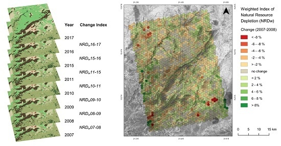
Figure 4 shows the design of the study: Based on the eight SAR images eight LULC classifications have been derived. The weighted index for Natural Resource Depletion is then calculated per image pair. The result is shown as an example for the first image pair of 2007 and 2008. This map indicates the spatial distribution of changes as well as their estimated impact on natural environment.
2.5. Index of Landscape Variability
Besides observing inter-annual changes, general conclusions about developments within an area can be derived best based on direct comparisons of conditions at the beginning and the end of the investigated time. However, this excludes two major points in change detection.
Firstly, savanna ecosystems are subject of large biotic and abiotic variation at multiple spatiotemporal scales [106]. It is a key task of remote sensing to reveal these variations to an adequate degree [107]. Besides simply comparing the intensity of changes, information on the temporal variability of regions—or in other words, the sum of all changes along the investigated period—has to be communicated as well. Surely, some areas remain stable after the transition of one LULC class into another while others tend to underlie regular variations. Analyzing changes over multiple images, especially in a region at the border between two ecosystems, surely should include the aspect of resilience towards long-term exterior influences.
Secondly, class-based measurements are always subject to smaller misclassifications, especially if the data source is challenging. It is still widely reported that classifications based on SAR data alone are outperformed by approaches using multispectral optical data [108,109,110]. Similarly, single misclassifications within a time-series can distort the results towards changes which did not happen. In addition to that, the dates of image acquisitions are highly sensitive towards seasonal variations. Even if all images were taken at the same date of the year, inter-annual shifts in phenology of even a few weeks could cause the erroneous detection of ‘pseudo changes’.
Consequently, a second indicator is needed which spatially allocates high temporal variation within the study area and simultaneously quantifies the number of smaller changes which might only be subject to seasonal shifts in phenology.
We therefore decided to apply a post-classification change vector analysis. Vector-based approaches make use of a feature space consisting of spectral or classified information and the temporal dimension [111,112]. In our case, the variable determining the value of each hexagon grid cell is its weighted sum of natural resources as described in the previous section. These values are then plotted against the temporal period which is analyzed as exemplified in Figure 5: In a first step, the length of the vector describing overall change (Co) is calculated based on the NR values of 2007 and 2017. As a second variable contributing to the variability of an area, the length of the change vectors between each chronological image pairs are summed up to create the sum of annual changes (Ca). For reasons of normalization, a factor of 10 has been applied to NR values for the calculation of vector lengths (e.g., a NR decrease of 0.55 to 0.40 during one year leads to a x-distance of 1.5 instead of 0.15. This is done because the y-distance is 1 except for 2011–2015). The ratio of Co and Ca is then calculated and describes the variability (v) of the corresponding hexagon cell throughout the observed period. If Co and Ca are of same length, v gets the value of 1. The longer the vectors of annual changes in relation to the overall change, the higher is the calculated variability v which is therefore a dimensionless value between 0 and 7, as the sum of the maximum NR value of 1 for a period of seven investigated years. This information can then be included in the discussion of the results as an indicator of variability and instability of an area.
3. Results
3.1. Annual Changes
3.1.1. Natural Resources
The results gathered based on the LULC classifications were transferred into NR for a hexagon grid as described in Section 2.4. A summary of different statistics over all 1793 grid cells is given in Table 6. It shows that overall resources did not significantly decline within the study area during the investigated period. Neither their mean (NRmean) nor their median (NRmedian) shows significant trends. A smaller drop of NRmedian can be observed for 2015. This indicates that natural resources were slightly the lowest in that year or at least at the time of image acquisition. This is supported by the value of the overall sum of all Natural Resources (NRsum). However, the percentiles of 95% and 5% (NR95% and NR5%) indicate that this could also have been caused by a smaller proportion of outliers for the year 2015.
A small decline in the maximum NR value (NRmax) reached can be observed as it decreases from 91.9% to 88.6% over the investigated period. The minimum (NRmin) was constant each year as it represents cells which are completely covered by bare rock—this being the class with the lowest attributed importance (see Table 5).
Overall, no significant change can be observed for the investigated area. A spatially explicit description of changes based on the weighted Natural Resource Depletion is presented in Section 3.1.2.
3.1.2. Natural Resource Depletion
Based on the derivation of NR values for each grid cell their impact upon environmental integrity (EnvInt, 35%) and human security (HumSec, 65%) can be estimated. Their summarized temporal development is demonstrated in Table 6: The mean change of resources (NRDw mean) ranges between +0.379% (2015–2016) and −0.421% (2011–2015). This means that positive and negative changes widely balance within the study area. At no time are changes dominated in one direction only. This is even more clearly shown by the median, which is not given in the table, as it levels at 0.0 throughout all years. Still, there are some years which show a slightly higher impact than others. If the NRDw values of all grid cells are added together per year (NRDw net), values between 6.79 and −7.55 emerge. These reveal a more distinct view on the impact of changes over time. While the overall changes in the study area are around ±3, a more pronounced impact of −7.55 can be assigned to the period between 2011 and 2015 as a consequence of missing data for an annual change detection.
However, the large increase between 2015 and 2016 (+6.79) indicates that the remarkably low value in 2015 of (−7.55) is not only caused by the longer time span but also depicts a local negative peak which needs to be discussed in Section 4.
The main advantage of the NRDw is that a value of percentaged increase or decrease of landscape quality can be assigned to each grid cell. This allows for the spatial characterization of landscape changes and their impacts. The results are provided as maps for the image pairs throughout the investigated period as demonstrated in Figure 6. It shows where the environment within the study area changed during the investigated years and in which directions changes occured regarding the expert-based weights shown in Table 5. At a first impression, no clear trends can be recognized in the maps. In particular, the regions around Camp Djabal and Goz Beïda show no considerable decrease in environmental resources during the last ten years. Also, the Hadjer Arkop massif is predominantly stable during the investigated period. Variations in NR can well be observed around Wadi Aouada and its areas of higher and more developed vegetation. Whether these are just of seasonal nature or a steady development cannot be clarified by comparing single conditions within time-series. This will be addressed more specifically in Section 3.2. In general, the areas of strongest developments are shrubland in the Southeast of the study area and grassland-covered plains in the North.
3.2. Overall Change and Variability of Natural Resources
As indicated in Section 2.5, attentive interpretation of change intensities requires information on the variability of the different grid cells. If an area shows moderate change between 2007 and 2017, but a high variability, as derived according to Figure 5, this area is either subject to higher intra-annual or inter-annual seasonal changes or to generally observable instabilities regarding the interrelations between related types of land cover (such as shrubland or grassland). In turn, if a low variability (smaller than 1.5) can be observed, changes are rather of long-term nature, such as trends in vegetation cover or transitions between types of land-use (bare soil to built-up areas). Figure 7 shows the changes as assessed by the NRDw between 2007 and 2017 in combination with the variability v per grid cell. While colors indicate the direction and severity of changes, line signatures within the grid cells indicate their variability. Developments can now be interpreted regarding their long-term information content and the affinity of an area towards changes. The indications from Section 3.1.2 can be affirmed and specified: There is no general loss of natural resources in the study area but certain areas are more prone to change than others. Areas around the settlements are almost stable whereas grids of both positive and negative development are accumulated at the South East of the study area. These result from the transition between forest and shrubland. Variability values of mostly above 2.00 indicate that this area is not gradually changing but generally prone to changes. Similar developments can be attached to Wadi Aouada where forest, shrubland, and grassland underlie both seasonal and inter-annual changes.
General conclusions about the study area can be drawn based on the statistical distribution of the different variability values compared to their NRDw value as shown in Figure 8. It clearly demonstrates that areas of smaller variability (v < 2.00) form the majority in the study area whereas areas with distinctively high variability (v > 4.00) are very rare. It furthermore shows that areas with slight changes (±2%) are more frequent than areas with no change at all, especially for higher variabilities. This indicates that many areas within the study area are affected by smaller changes and show a relatively unsteady development. It is additionally interesting that areas of highest positive development (>8%) increase with larger variability. This leads to the conclusion that some of them may also result from misclassifications as the classes of high variability no longer show an equal distribution.
4. Discussion
Altogether, the proposed approach allows the derivation of detailed change maps along a series of SAR images which exceed the information content of standard transition matrices between classes. However, there are things to notice in both the ecologic and methodic domain. This section aggregates our findings in the perspective of landscape development and according to the requirements defined in the introduction.
4.1. Landscape Changes
One main point to report is that the landscape in the study area did not underlie large-scale changes, neither positively nor negatively. As shown in Figure 6, there in fact are certain hot spots of accumulated change over the investigated period, however, these did not add up to a gradual overall increase or decrease of landscape quality for larger areas.
Addressing anthropogenic impact on the investigated landscape, neither of the two main settlements of camp Djabal and the city of Goz Beïda, nor the plains within the Hadjer Arkop massif, had noticeable impact on their surrounding landscapes. These findings were expected in terms of no reported growth of these settlements during the investigated period [113,114,115]. It is still notable that this landscape did not negatively respond to the direct presence of human activities as arid savannas are often observed to be susceptible towards anthropogenic pressure [116]. One reason for the described stability within this area is the high amount of bare soil as a consequence of the relatively intensive agricultural use. Accordingly, their NR values were already quite low and only expansion of human settlements—or the transition from soil areas to bare rock—would have caused negative NRDw developments. In addition to that, no source of land degradation or desertification, as it might be indicated by transitions from vegetation to bare soil or soil to rock, could be observed among the bare rock areas of the Hadjer Arkop massif.
One region which was prone to many changes during the investigated period is Wadi Aouada, reaching from the West to the North of the study area. As it is the only area with vital vegetation of higher orders during the whole year, it is particularly prone to changes in external circumstances. A direct comparison of the NR of 2007 with 2017 (Figure 7) does not depict a clear image on which parts of the wadi underlay significant positive or negative developments. It can, however, be stated that the core area of the wadi did not change in a critical degree—for example, due to erosion or lesser subsurface drainage. Looking at the annual changes in Figure 6 indicates that there are some years where the wadi is subject to larger changes, notably 2008–2009 (positive) and 2010–2011 (negative). These observations could be linked to climatic variations. However, comparison to records of temperature and precipitation provided by the Climatic Research Unit (CRU) of University of East Anglia (UEA) [117] does not confirm these trends. As Figure 9 shows, the contrary could have been expected as a considerable decrease in precipitation occurred between 2008 and 2009, which in turn shows the most visible positive development within Wadi Aouada. So it can be concluded that climatic variations are most likely not responsible for the smaller changes within the wadi. We expect them to result from overall variation in the vegetation signature within the SAR data.
Another mentionable point is the striking accumulation of negative NRDw values in for 2011–2015 in the North of the Hadjer Arkop massif near the center of the study area. However, the fact that this area is again strikingly positive for the subsequent image pair from 2015–2016 indicates that this anomaly is rather the outcome of a wrong classification. The low variability values in this area (Figure 7) furthermore support this indication and lead to the conclusion that this area is in fact stable regarding LULC and the assessed changes are wrong. Nevertheless, many larger changes for the period from 2011–2015 are realistic results obtained by the observed increment of 4 years instead of one. But this is one example of how investigating variabilities along a time-series can help to detect errors and check the results for plausibility.
To further test the overall condition of the landscape for interrelations with climatic conditions, we compared the sum of all NRDw values per year, (NRDw net), with the corresponding change in annual precipitation (Δprec) as shown in Table 7. We found a Pearson correlation coefficient of r = 0.47 between both variables which affirms that overall sum of natural resources could in fact fluctuate to a certain degree according to the water availability in the study area. A correlation of r = −0.61 was found for the relationship between NRDw net and the temporal baseline between the respective SAR images (SAR Δd), defined as the absolute difference in days from an optimum temporal difference between two images of 365 days. It seems obvious that potential changes increase if both images are not taken on the same day of the year. The larger the difference of two images regarding their time of acquisition (see Table 1), the higher is the risk of identifying changes related to phenology instead of identifying changes to overall development of a landscape.
Lastly, the histogram in Figure 8 demonstrates how changes in the image can be interpreted regarding their long-term predication. Overall changes with low variabilities (between 1.00 and 1.50) make up 72% in our study. If frequencies are not equally distributed in both positive and negative directions, trends can be evaluated regarding their variability. We found that high variability values either indicate single misclassifications between scenes or, when spatially aggregated, characterize areas of constant change. In the latter case, intensities of changes should be interpreted with more care.
4.2. Methods
On the technical side the following points can be highlighted. As the first findings made by Braun et al. [23] indicated, the application of the NRDw concept from Hagenlocher et al. [104] is transferable to radar imagery of medium spatial resolution. This study was able to provide a framework more robust towards smaller misclassifications as they often occur in SAR data which is still flexible enough to be based on different sensors or to be transferred to other regions. The results created reflect different aspects of landscape changes: namely environmental integrity and human security which can be weighted according to the expertise and the needs of the user. The final maps include information on both spatial and temporal variation of landscape changes but are still easy to read and interpret. These maps highlight regions which require special attention and allow a more differentiated dealing with the outcomes.
ALOS PALSAR proved to be suitable for long-term landscape monitoring due to its long wavelength interaction with volume scatterers for the discrimination of different types of vegetation. It would have been interesting to observe how the study area changed annually in this perspective between 2011 and 2015 but no accessible L-band data is available for this period. It is however expected that other SAR sensors with similar archives such as ERS, Radarsat, and Envisat bear the same potential, especially at the temporal scale. Regarding seasonality, additional data at the middle or end of the rainy season would surely have substantially increased the validity of the approach as it could have been used to depict a clearer image of each year’s resources. However, this data was not available for all the investigated years. Future approaches surely should consider using a combination of several scenes at crucial points in the study area’s phenology which can be determined by the variation of NDVI, for example [118,119,120]. This would also decrease the weight of textural information in favor of additional seasonal effects.
However, the used textures were able to discriminate all selected LULC classes to a sufficient degree. As Table 3 and Table 4 demonstrate, Grassland was the class with lowest accuracies due to its indifferent degree of coverage in the study area and comparably low interaction with the L-band signal. Using these large numbers of input rasters surely requires classifiers based on machine-learning which extract the most valuable information. The random forest classifier performed efficient but other approaches, such as support vector machines (SVM) or artificial neuronal networks (ANN), can be employed as well for these kinds of analyses, especially when phenological variation is additionally introduced as suggested above [121,122].
The automatic and literature-based selection of training areas proved to increase the study’s credibility as it reduces the possible bias of manual sampling collection. In our case, field investigations were not possible due to security reasons but using optical data from Landsat grants for independency of the training and validation process from the actual image classification was possible. Also worth noting, optical data does not have to be complete or cloud free. As only the areas which consistently fulfilled the criteria listed in Table 2 throughout all images were used for possible locations of the randomized samples, we could flexibly deal with cloud coverage, burnt areas and missing scan lines in Landsat ETM+ products.
Smaller misclassifications occurred between classes with similar response to the radar signal as shown in Table 3 and Table 4. These could, however, be compensated by the creation of hexagon grid cells as a main unit of analysis. Each of them aggregates information of 1280 pixels and represents their percentaged share as one value of natural resources. This reduces the effect of ambiguities at the transition between two LULC classes and facilitates both the visual inspection and interpretation of results. Detailed changes at borders between two classes are no longer visible in this approach but since the fact that savanna ecosystems often consist of a mosaic of continuous LULC this is neither possible nor considered as reasonable. Shifts in phenology could, however, been better handled with an investigation over a longer time span. The longer the time-series of images, the more stable is the approach as it more clearly reveals outliers along the investigated period. ESA’s Sentinel-1 mission lays a solid foundation for multi-decade investigations as it was designed to continue the archived data of ERS and Envisat. All of them operate at C-band wavelengths and a comparable spatial resolution.
One crucial point is the definition of investigated LULC classes and their corresponding contribution to both environmental integrity and human security (see Table 5). As this has to be done at the beginning of the study, changes in the numbers of investigated classes can, of course, strongly affect the later results. If interest is placed on the change of a certain type of LULC, the definition of classes should be appropriate and respectively balanced in this context. Also, the expert-based weights have large influence on the evaluation of the changes. It is therefore advisable to include the expertise of as many people as possible, preferably from different domains (local population, humanitarian units, authorities, and other stakeholders). This not only provides for a balanced assessment of weights but also prevents the abuse of weights to intentionally target desired results. As Laczko & Aghazarm argue, research on the impacts of refugee camps upon their environment is needed but cannot act as the only argument for repatriation in political debates [123].
Lastly, the proposed variability can be a valuable measure for both the quality and the long-term information content of results. However, a way of normalization has to be performed when comparing index values along a temporal sequence. We used a rather basic model of change vectors as it met our requirements for the comparison of eight images. If longer or more detailed time-series are employed, the concept of variability has to be refined according to variation at different temporal scales—such as the differentiation between seasonal, inter-annual, and overall variation of a grid cell.
5. Conclusions
Our study showed that landscape changes can be analyzed by radar imagery in a transparent and adaptive way. It is not limited to certain landscape types or specific sensors, but requires a minimum number of consecutive images from the same time of the year. The proposed approach substantially contributes to field of post-classification change analysis as it overcomes limitations regarding the number of investigated scenes, the variation within the investigated time, and the occasionally criticized complexity of high-level approaches which cannot be adapted by users with limited technical or scientific background. It therefore serves as an ideal intermediate between innovative analyses and user-friendly, adaptable frameworks. These will gain further importance with the growing availability of archived and newly acquired SAR data for scientific, organizational, and commercial operational use.
The integration of user expertise about the relevance of land-use and land cover classes hinders the automation of the process but clearly improves the validity of the results. Attaching weights to the selected classes allows for the generation of an index which refines the results according to the knowledge of the user and the information he requires.
Although it did not reveal large scale trends in our study area, the proposed index is a good approach for a semi-automated evaluation of changes over long time spans and within greater regions. The use of radar data additionally reduces the dependency from atmospherically undisturbed conditions. All parts of the study were performed on free and open source tools (QGIS, ESA SNAP, OTB, Python) which allows for a transfer of the method onto other case areas. We encourage readers to implement and further improve the proposed approach in order to increase the quality of time-series analyses of radar data. This work is a first step towards new standards in change detection applications which are comprehensible and still specified to the users’ needs.
Acknowledgments
This study was funded by the Austrian Research Promotion Agency (FFG) under the Austrian Space Applications Programme (ASAP 12, 854041). ALOS data was provided by Japan Aerospace Exploration Agency (JAXA). Landsat and SRTM data was provided by the US Geological Survey (USGS). The authors would like to thank Ted Cahill for proofreading the manuscripts and the anonymous reviewers for their valuable comments and suggestions to improve the manuscript. We acknowledge support by Deutsche Forschungsgemeinschaft and Open Access Publishing Fund of University of Tübingen.
Author Contributions
Andreas Braun and Volker Hochschild designed the study and selected the data; Andreas Braun processed and analyzed the data; Results were interpreted and discussed by Andreas Braun and Volker Hochschild The manuscript was submitted, edited and revised by Andreas Braun
Conflicts of Interest
The authors declare no conflict of interest.
References
- Irons, J.R.; Dwyer, J.L.; Barsi, J.A. The next Landsat satellite: The Landsat data continuity mission. Remote Sens. Environ. 2012, 122, 11–21. [Google Scholar] [CrossRef]
- Wulder, M.A.; White, J.C.; Goward, S.N.; Masek, J.G.; Irons, J.R.; Herold, M.; Cohen, W.B.; Loveland, T.R.; Woodcock, C.E. Landsat continuity: Issues and opportunities for land cover monitoring. Remote Sens. Environ. 2008, 112, 955–969. [Google Scholar] [CrossRef]
- Byrne, G.F.; Crapper, P.F.; Mayo, K.K. Monitoring land-cover change by principal component analysis of multitemporal landsat data. Remote Sens. Environ. 1980, 10, 175–184. [Google Scholar] [CrossRef]
- Fung, T. An Assessment of TM Imagery for Land-cover Change Detection. IEEE Trans. Geosci. Remote Sens. 1990, 28, 681–684. [Google Scholar] [CrossRef]
- Guerschman, J.P.; Paruelo, J.M.; Di Bella, C.; Giallorenzi, M.C.; Pacin, F. Land cover classification in the Argentine Pampas using multi-temporal Landsat TM data. Int. J. Remote Sens. 2003, 24, 3381–3402. [Google Scholar] [CrossRef]
- Yuan, F.; Sawaya, K.E.; Loeffelholz, B.C.; Bauer, M.E. Land cover classification and change analysis of the Twin Cities (Minnesota) Metropolitan Area by multitemporal Landsat remote sensing. Remote Sens. Environ. 2005, 98, 317–328. [Google Scholar] [CrossRef]
- Bakr, N.; Weindorf, D.C.; Bahnassy, M.H.; Marei, S.M.; El-Badawi, M.M. Monitoring land cover changes in a newly reclaimed area of Egypt using multi-temporal Landsat data. Appl. Geogr. 2010, 30, 592–605. [Google Scholar] [CrossRef]
- Zhu, Z.; Woodcock, C.E.; Holden, C.; Yang, Z. Generating synthetic Landsat images based on all available Landsat data: Predicting Landsat surface reflectance at any given time. Remote Sens. Environ. 2015, 162, 67–83. [Google Scholar] [CrossRef]
- Masek, J.G.; Huang, C.; Wolfe, R.; Cohen, W.; Hall, F.; Kutler, J.; Nelson, P. North American forest disturbance mapped from a decadal Landsat record. Remote Sens. Environ. 2008, 112, 2914–2926. [Google Scholar] [CrossRef]
- He, L.; Chen, J.M.; Zhang, S.; Gomez, G.; Pan, Y.; McCullough, K.; Birdsey, R.; Masek, J.G. Normalized algorithm for mapping and dating forest disturbances and regrowth for the United States. Int. J. Appl. Earth Obs. Geoinf. 2011, 13, 236–245. [Google Scholar] [CrossRef]
- Song, C.; Woodcock, C.E.; Seto, K.C.; Lenney, M.P.; Macomber, S.A. Classification and change detection using Landsat TM data: When and how to correct atmospheric effects? Remote Sens. Environ. 2001, 75, 230–244. [Google Scholar] [CrossRef]
- Warren, S.G.; Hahn, C.J.; London, J.; Chervin, R.; Jenne, R.L. Global Distribution of Total Cloud Cover and Cloud Type Amounts over Land. NCAR Tech. Note TN-273+STR. Available online: http://opensky.ucar.edu/islandora/object/technotes%3A444/datastream/PDF/download/citation.pdf (accessed on 22 November 2016).
- Gu, G.; Zhang, C. Cloud components of the Intertropical Convergence Zone. J. Geophys. Res. 2002, 107. [Google Scholar] [CrossRef]
- Kummerow, C.; Barnes, W.; Kozu, T.; Shiue, J.; Simpson, J. The Tropical rainfall measuring mission (TRMM) sensor package. J. Atmos. Ocean. Technol. 1998, 15, 809–817. [Google Scholar] [CrossRef]
- Kummerow, C.; Simpson, J.; Thiele, O.; Barnes, W.; Chang, A.T.C.; Stocker, E.; Adler, R.F.; Hou, A.; Kakar, R.; Wentz, F.; et al. The status of the tropical rainfall measuring mission (TRMM) after two years in orbit. J. Appl. Meteorol. 2000, 39, 1965–1982. [Google Scholar] [CrossRef]
- Asner, G.P. Cloud cover in Landsat observations of the Brazilian Amazon. Int. J. Remote Sens. 2001, 22, 3855–3862. [Google Scholar] [CrossRef]
- Mas, J.-F. Monitoring land-cover changes: A comparison of change detection techniques. Int. J. Remote Sens. 1999, 20, 139–152. [Google Scholar] [CrossRef]
- Ju, J.; Roy, D.P. The availability of cloud-free Landsat ETM+ data over the conterminous United States and globally. Remote Sens. Environ. 2008, 112, 1196–1211. [Google Scholar] [CrossRef]
- Fletcher, K. ERS Missions. 20 Years of Observing Earth; ESA Communications: Noordwijk, The Netherlands, 2013. [Google Scholar]
- Flett, D.; Crevier, Y.; Girard, R. The RADARSAT Constellation Mission: Meeting the government of Canada’S needs and requirements. In Proceedings of the 2009 IEEE International Geoscience and Remote Sensing Symposium, Cape Town, South Africa, 12–17 July 2009. [Google Scholar]
- Torres, R.; Snoeij, P.; Geudtner, D.; Bibby, D.; Davidson, M.; Attema, E.; Potin, P.; Rommen, B.; Floury, N.; Brown, M.; et al. GMES Sentinel-1 mission. Remote Sens. Environ. 2012, 120, 9–24. [Google Scholar] [CrossRef]
- Liew, S.C.; Kam, S.P.; Tuong, T.P.; Chen, P.; Minh, V.Q.; Lim, H. Landcover classification over the Mekong river delta using ERS and RADARSAT SAR images. In Proceedings of the 1997 IEEE International Geoscience and Remote Sensing Symposium, Remote Sensing—A Scientific Vision for Sustainable Development, Singapore, 3–8 August 1997. [Google Scholar]
- Braun, A.; Lang, S.; Hochschild, V. Impact of refugee camps on their environment a case study using multi-temporal SAR data. J. Geogr. Environ. Earth Sci. Int. 2016, 4, 1–17. [Google Scholar] [CrossRef]
- McAvoy, J.G.; Krakowskii, E.M. A Knowledge based system for the interpretation of SAR Images of sea ice. In Proceedings of the 12th Canadian Symposium on Remote Sensing Geoscience and Remote Sensing Symposium, Vancouver, BC, Canada, 10–14 July 1989. [Google Scholar]
- Pierce, L.E.; Ulaby, F.T.; Sarabandi, K.; Dobson, M.C. Knowledge-based classification of polarimetric SAR images. IEEE Trans. Geosci. Remote Sens. 1994, 32, 1081–1086. [Google Scholar] [CrossRef]
- Dobson, M.C.; Pierce, L.E.; Ulaby, F.T. Knowledge-based land-cover classification using ERS-1/JERS-1 SAR composites. IEEE Trans. Geosci. Remote Sens. 1996, 34, 83–99. [Google Scholar] [CrossRef]
- Nunnally, N.R. Integrated landscape analysis with radar imagery. Remote Sens. Environ. 1969, 1, 1–6. [Google Scholar] [CrossRef]
- Askne, J.; Hagberg, J.O. Potential of interferometric SAR for classification of land surfaces. In Proceedings of the IEEE International Geoscience and Remote Sensing Symposium, Tokyo, Japan, 18–21 August 1993. [Google Scholar]
- Dutra, L.V. Feature extraction and selection for ERS-1/2 InSAR classification. Int. J. Remote Sens. 1999, 20, 993–1016. [Google Scholar] [CrossRef]
- Engdahl, M.E.; Hyyppa, J.M. Land-cover classification using multitemporal ERS-1/2 insar data. IEEE Trans. Geosci. Remote Sens. 2003, 41, 1620–1628. [Google Scholar] [CrossRef]
- Huber, R.; Dutra, L.V. Feature selection for ERS-1/2 InSAR classification: High dimensionality case. In Proceedings of the 1998 IEEE International Geoscience and Remote Sensing, Seattle, WA, USA, 6–10 July 1998. [Google Scholar]
- Oliver, C.J. Rain forest classification based on SAR texture. IEEE Trans. Geosci. Remote Sens. 2000, 38, 1095–1104. [Google Scholar] [CrossRef]
- Bruzzone, L.; Marconcini, M.; Wegmuller, U.; Wiesmann, A. An advanced system for the automatic classification of multitemporal SAR images. IEEE Trans. Geosci. Remote Sens. 2004, 42, 1321–1334. [Google Scholar] [CrossRef]
- Van Zyl, J.J.; Burnette, C.F. Bayesian classification of polarimetric SAR images using adaptive a priori probabilities. Int. J. Remote Sens. 1992, 13, 835–840. [Google Scholar] [CrossRef]
- Rignot, E.; Williams, C.L.; Way, J.; Viereck, L.A. Mapping of forest types in Alaskan boreal forests using SAR imagery. IEEE Trans. Geosci. Remote Sens. 1994, 32, 1051–1059. [Google Scholar] [CrossRef]
- Chiang, H.-C.; Moses, R.L.; Potter, L.C. Model-based classification of radar images. IEEE Trans. Inf. Theory 2000, 46, 1842–1854. [Google Scholar] [CrossRef]
- Tzeng, Y.C.; Chen, K.S. A fuzzy neural network to SAR image classification. IEEE Trans. Geosci. Remote Sens. 1998, 36, 301–307. [Google Scholar] [CrossRef]
- Chen, C.-T.; Chen, K.-S.; Lee, J.-S. The use of fully polarimetric information for the fuzzy neural classification of SAR images. IEEE Trans. Geosci. Remote Sens. 2003, 41, 2089–2100. [Google Scholar] [CrossRef]
- Zhang, Y.; Wu, L.; Neggaz, N.; Wang, S.; Wei, G. Remote-sensing image classification based on an improved probabilistic neural network. Sensors 2009, 9, 7516–7539. [Google Scholar] [CrossRef] [PubMed]
- Van Beijma, S.; Comber, A.; Lamb, A. Random forest classification of salt marsh vegetation habitats using quad-polarimetric airborne SAR, elevation and optical RS data. Remote Sens. Environ. 2014, 149, 118–129. [Google Scholar] [CrossRef]
- Du, P.; Samat, A.; Waske, B.; Liu, S.; Li, Z. Random forest and rotation forest for fully polarized SAR image classification using polarimetric and spatial features. ISPRS J. Photogramm. Remote Sens. 2015, 105, 38–53. [Google Scholar] [CrossRef]
- Gupta, S.; Singh, D.; Singh, K.P.; Kumar, S. An efficient use of random forest technique for SAR data classification. In Proceedings of the 2015 IEEE International Geoscience and Remote Sensing Symposium, Milan, Italy, 26–31 July 2015. [Google Scholar]
- Lee, J.-S.; Grunes, M.R.; Kwok, R. Classification of multi-look polarimetric SAR imagery based on complex Wishart distribution. Int. J. Remote Sens. 1994, 15, 2299–2311. [Google Scholar] [CrossRef]
- Cloude, S.R.; Pottier, E. An entropy based classification scheme for land applications of polarimetric SAR. IEEE Trans. Geosci. Remote Sens. 1997, 35, 68–78. [Google Scholar] [CrossRef]
- Alberga, V. A study of land cover classification using polarimetric SAR parameters. Int. J. Remote Sens. 2007, 28, 3851–3870. [Google Scholar] [CrossRef]
- Qi, Z.; Yeh, A.G.-O.; Li, X.; Lin, Z. A novel algorithm for land use and land cover classification using RADARSAT-2 polarimetric SAR data. Remote Sens. Environ. 2012, 118, 21–39. [Google Scholar] [CrossRef]
- White, R.G. Change detection in SAR imagery. Int. J. Remote Sens. 1991, 12, 339–360. [Google Scholar] [CrossRef]
- Rignot, E.; van Zyl, J.J. Change detection techniques for ERS-1 SAR data. IEEE Trans. Geosci. Remote Sens. 1993, 31, 896–906. [Google Scholar] [CrossRef]
- Bazi, Y.; Bruzzone, L.; Melgani, F. An unsupervised approach based on the generalized Gaussian model to automatic change detection in multitemporal SAR images. IEEE Trans. Geosci. Remote Sens. 2005, 43, 874–887. [Google Scholar] [CrossRef]
- Dekker, R.J. Speckle filtering in satellite SAR change detection imagery. Int. J. Remote Sens. 1998, 19, 1133–1146. [Google Scholar] [CrossRef]
- Bovenga, F.; Refice, A.; Nutricato, R.; Pasquariello, G.; de Carolis, G. Automated calibration of multi-temporal ERS SAR data. In Proceedings of the IEEE International Geoscience and Remote Sensing Symposium, Toronto, ON, Canada, 24–28 June 2002. [Google Scholar]
- Townsend, P.A.; Foster, J.R. A synthetic aperture radar-based model to assess historical changes in lowland floodplain hydroperiod. Water Resour. Res. 2002, 38, 20-1–20-10. [Google Scholar] [CrossRef]
- Beisl, C.H.; de Miranda, F.P.; Evsukoff, A.G.; Pedroso, E.C. Assessment of environmental sensitivity index of flooding areas in western Amazonia using fuzzy logic in the dual season GRFM JERS-1 SAR image mosaics. In Proceedings of the 2003 IEEE International Geoscience and Remote Sensing Symposium, Toulouse, France, 21–25 July 2003. [Google Scholar]
- Hoffmann, A.A.; Siegert, F.; Hinrichs, A. Fire Damage in East Kalimantan in 1997/98 Related to Land Use and Vegetation Classes. Satellite Radar Inventory Results and Proposals for Further Actions; IFFM/SFMP: Samarinda, Indonesia, 1987. [Google Scholar]
- Saatchi, S.S.; Soares, J.V.; Alves, D.S. Mapping deforestation and land use in amazon rainforest by using SIR-C imagery. Remote Sens. Environ. 1997, 59, 191–202. [Google Scholar] [CrossRef]
- Strozzi, T.; Wegmuller, U.; Luckman, A.; Balzter, H. Mapping deforestation in Amazon with ERS SAR interferometry. In Proceedings of the IEEE 1999 International Geoscience and Remote Sensing Symposium, Hamburg, Germany, 28 June–2 July 1999. [Google Scholar]
- Almeida-Filho, R.; Rosenqvist, A.; Shimabukuro, Y.E.; Dos Santos, J.R. Evaluation and perspectives of using multitemporal L-Band SAR data to monitor deforestation in the Brazilian Amazonia. IEEE Geosci. Remote Sens. Lett. 2005, 2, 409–412. [Google Scholar] [CrossRef]
- Almeida-Filho, R.; Shimabukuro, Y.E.; Rosenqvist, A.; Sánchez, G.A. Using dual-polarized ALOS PALSAR data for detecting new fronts of deforestation in the Brazilian Amazônia. Int. J. Remote Sens. 2009, 30, 3735–3743. [Google Scholar] [CrossRef]
- Ryan, C.M.; Hill, T.; Woollen, E.; Ghee, C.; Mitchard, E.; Cassells, G.; Grace, J.; Woodhouse, I.H.; Williams, M. Quantifying small-scale deforestation and forest degradation in African woodlands using radar imagery. Glob. Chang. Biol. 2012, 18, 243–257. [Google Scholar] [CrossRef]
- Mitchard, E.T.A.; Saatchi, S.S.; Woodhouse, I.H.; Nangendo, G.; Ribeiro, N.S.; Williams, M.; Ryan, C.M.; Lewis, S.L.; Feldpausch, T.R.; Meir, P. Using satellite radar backscatter to predict above-ground woody biomass: A consistent relationship across four different African landscapes. Geophys. Res. Lett. 2009. [Google Scholar] [CrossRef]
- Mitchard, E.; Saatchi, S.S.; Lewis, S.L.; Feldpausch, T.R.; Woodhouse, I.H.; Sonké, B.; Rowland, C.; Meir, P. Measuring biomass changes due to woody encroachment and deforestation/degradation in a forest–savanna boundary region of central Africa using multi-temporal L-band radar backscatter. Remote Sens. Environ. 2011, 115, 2861–2873. [Google Scholar] [CrossRef]
- Shen, G.; Liao, J.; Zhang, L.; Li, X. Wetland landscape analysis using polarimetric RADARSAT-2 data. In Proceedings of the 2014 IEEE International Geoscience and Remote Sensing Symposium, Quebec City, QC, Canada, 13–18 July 2014. [Google Scholar]
- Tewkesbury, A.P.; Comber, A.J.; Tate, N.J.; Lamb, A.; Fisher, P.F. A critical synthesis of remotely sensed optical image change detection techniques. Remote Sens. Environ. 2015, 160, 1–14. [Google Scholar] [CrossRef]
- Hussain, M.; Chen, D.; Cheng, A.; Wei, H.; Stanley, D. Change detection from remotely sensed images: From pixel-based to object-based approaches. ISPRS J. Photogramm. Remote Sens. 2013, 80, 91–106. [Google Scholar] [CrossRef]
- Walker, P.A.; Peters, P.E. Making Sense in Time: Remote Sensing and the Challenges of Temporal Heterogeneity in Social Analysis of Environmental Change. Hum. Ecol. 2007, 35, 69–80. [Google Scholar] [CrossRef]
- Hauck, J.; Görg, C.; Varjopuro, R.; Ratamäki, O.; Maes, J.; Wittmer, H.; Jax, K. “Maps have an air of authority”: Potential benefits and challenges of ecosystem service maps at different levels of decision making. Ecosyst. Serv. 2013, 4, 25–32. [Google Scholar] [CrossRef]
- Kienberger, S.; Füreder, P.; Hölbling, D.; Tiede, D.; Contreras Mojica, D.M.; Hagenlocher, M.; Zeil, P.; Lang, S. Von Geodaten zu nutzbarer Geoinformation: Entwicklung von und Anforderung an kartografische Produkte im Katastrophenmanagement-Zyklus. In Proceedings of the Workshop “Raum Zeit Risiko”, München, Germany, 28 November 2013. [Google Scholar]
- Ariti, A.T.; van Vliet, J.; Verburg, P.H. Land-use and land-cover changes in the Central Rift Valley of Ethiopia: Assessment of perception and adaptation of stakeholders. Appl. Geogr. 2015, 65, 28–37. [Google Scholar] [CrossRef]
- Hansen, K.F. Chad. In Africa Yearbook Volume 11; Elischer, S., Mehler, A., Hofmeier, R., Melber, H., Eds.; Brill: Leiden, The Netherlands, 2015; pp. 201–208. [Google Scholar]
- Rishmawi, K.; Prince, S. Environmental and anthropogenic degradation of vegetation in the Sahel from 1982 to 2006. Remote Sens. 2016. [Google Scholar] [CrossRef]
- Southworth, J.; Zhu, L.; Bunting, E.; Ryan, S.J.; Herrero, H.; Waylen, P.R.; Hill, M.J. Changes in vegetation persistence across global savanna landscapes, 1982–2010. J. Land Use Sci. 2014, 11, 7–32. [Google Scholar] [CrossRef]
- Office for the Coordination of Humanitarian Affairs (OCHA). Profil Régional du Sila: Novembre 2012. Available online: https://docs.unocha.org/sites/dms/CHAD/Profil_Dar%20Sila_Novembre%202012.pdf (accessed on 8 December 2016).
- Clark, J.; Tan, V. Hundreds Flee New Fighting in Darfur; UNHCR Opens 8th Camp in Chad. Available online: http://www.unhcr.org/print/40c081119.html (accessed on 15 November 2016).
- Bouchardy, J.-Y. Radar Images and Geographic Information Helping Identify Water Resources during Humanitarian Crisis: The Case of Chad/Sudan (Darfur) Emergency. In Global Monitoring for Sustainability and Security, Proceedings of the 31st International Symposium of Remote Sensing & the Environment, St. Petersburg, Russian, 20–24 June 2005; Bobylev, L.P., Ed.; International Center for Remote Sensing of Environment: Berlin, Germany, 2005. [Google Scholar]
- Humanitarian Information Unit. Sudan (Darfur) and Chad Border Region: Confirmed Damaged and Destroyed Villages. Available online: http://reliefweb.int/map/sudan/sudan-darfur-and-chad-border-region-confirmed-damaged-and-destroyed-villages-2-august-2004 (accessed on 14 November 2016).
- Middleton, N.; Thomas, D.S.G. World Atlas of Desertification, 2nd ed.; Arnold: London, UK, 1997. [Google Scholar]
- Harris, I.; Jones, P.D.; Osborn, T.J.; Lister, D.H. Updated high-resolution grids of monthly climatic observations—The CRU TS3.10 Dataset. Int. J. Climatol. 2014, 34, 623–642. [Google Scholar] [CrossRef]
- Funk, C.; Rowland, J.; Eilerts, G.; Adoum, A.; White, L. A Climate Trend Analysis of Chad: Famine Early Warning Systems Network—Informaing Climate Change Adaption Series; FEWSNET/US Geological Survey Fact Sheet 2012–3070; U.S. Geological Survey: Reston, VA, USA, 2012.
- Brownfield, M.E. Assessment of undiscovered oil and gas resources of the sud province, Central East Africa. In Geologic Assessment of Undiscovered Hydrocarbon Resources of Sub-Saharan Africa; Brownfield, M.E., Ed.; U.S. Geological Survey: Reston, VA, USA, 2011. [Google Scholar]
- Pias, J. Les formations tertiaires et quaternaires de la cuvette tchadienne (République du Tchad). In Congrès Panafricain de Préhistoire et de L’étude du Quaternaire; Dakar: Bondy, France, 1976; pp. 425–429. [Google Scholar]
- White, F. Vegetation Map of Africa. A Descriptive Memoir to Accompany the Unesco/AETFAT/UNSO Vegetation Map of Africa; Unesco: Paris, France, 1981. [Google Scholar]
- Wickens, G.E. The Flora of Jebel Marra (Sudan Republic) and Its Geographical Affinities; H.M. Stationery Off.: London, UK, 1976. [Google Scholar]
- Ministerie van Defensie. European Union Force Chad/CAR. Available online: https://www.defensie.nl/binaries/defence/documents/leaflets/2013/02/05/european-union-force-chad-car-pdf/european-union-force-chad-car-pdf.pdf (accessed on 8 December 2016).
- Markham, B.L.; Storey, J.C.; Williams, D.L.; Irons, J.R. Landsat sensor performance: History and current status. IEEE Trans. Geosci. Remote Sens. 2004, 42, 2691–2694. [Google Scholar] [CrossRef]
- JAXA. ALOS/PALSAR Level 1.1/1.5 Product Format Description. NEB-070062B. Available online: http://www.eorc.jaxa.jp/ALOS/en/doc/fdata/PALSAR_x_Format_EL.pdf (accessed on 5 April 2017).
- JAXA. ALOS-2/PALSAR-2 Level 1.1/1.5 Product Format Description. Ü129-132. Available online: http://www.eorc.jaxa.jp/ALOS-2/en/doc/fdata/PALSAR-2_xx_Format_CEOS_E_r.pdf (accessed on 5 April 2017).
- Shimada, M.; Isoguchi, O.; Tadono, T.; Isono, K. PALSAR Radiometric and Geometric Calibration. IEEE Trans. Geosci. Remote Sens. 2009, 47, 3915–3932. [Google Scholar] [CrossRef]
- Small, D. Flattening Gamma: Radiometric Terrain Correction for SAR Imagery. IEEE Trans. Geosci. Remote Sens. 2011, 49, 3081–3093. [Google Scholar] [CrossRef]
- Loew, A.; Mauser, W. Generation of geometrically and radiometrically terrain corrected SAR image products. Remote Sens. Environ. 2007, 106, 337–349. [Google Scholar] [CrossRef]
- Collins, M.J.; Wiebe, J.; Clausi, D.A. The effect of speckle filtering on scale-dependent texture estimation of a forested scene. IEEE Trans. Geosci. Remote Sens. 2000, 38, 1160–1170. [Google Scholar] [CrossRef]
- Prasad, T.S.; Gupta, R.K. Texture based classification of multidate SAR images—A case study. Geocarto Int. 1998, 13, 53–62. [Google Scholar] [CrossRef]
- Haralick, R.M.; Shanmugam, K.; Dinstein, I. Textural Features for Image Classification. IEEE Trans. Syst. Man Cybern. 1973, 3, 610–621. [Google Scholar] [CrossRef]
- Chander, G.; Markham, B.L.; Helder, D.L. Summary of current radiometric calibration coefficients for Landsat MSS, TM, ETM+, and EO-1 ALI sensors. Remote Sens. Environ. 2009, 113, 893–903. [Google Scholar] [CrossRef]
- Moran, M.; Jackson, R.D.; Slater, P.N.; Teillet, P.M. Evaluation of simplified procedures for retrieval of land surface reflectance factors from satellite sensor output. Remote Sens. Environ. 1992, 41, 169–184. [Google Scholar] [CrossRef]
- Forkuor, G.; Landmann, T.; Conrad, C.; Dech, S. Agricultural land use mapping in the sudanian savanna of West Africa: Current status and future possibilities. In Proceedings of the 2012 IEEE International Geoscience and Remote Sensing Symposium, Munich, Germany, 22–27 July 2012. [Google Scholar]
- Guiguindibaye, M.; Belem, M.O.; Boussim, J.L.; Ndoutorlengar, M. Effect of early fires on the behavior of some perennial woody and herbaceous species in Sudan savanna in chad. Indian J. Sci. Res. Technol. 2015, 3, 56–65. [Google Scholar]
- López-García, M.J.; Caselles, V. Mapping burns and natural reforestation using thematic Mapper data. Geocarto Int. 1991, 6, 31–37. [Google Scholar] [CrossRef]
- Drury, S.A. Image Interpretation in Geology, 3rd ed.; Blackwell Science: Malden, MA, USA, 2001. [Google Scholar]
- Liu, J.; Heiskanen, J.; Aynekulu, E.; Maeda, E.; Pellikka, P. Land Cover Characterization in West Sudanian Savannas Using Seasonal Features from Annual Landsat Time Series. Remote Sens. 2016. [Google Scholar] [CrossRef]
- Hartigan, J.A.; Wong, M.A. Algorithm AS 136: A K-Means Clustering Algorithm. Appl. Stat. 1979, 28, 100. [Google Scholar] [CrossRef]
- Fisher, R.A. On an Absolute Criterion for Fitting Frequency Curves. Stat. Sci. 1912, 12, 39–41. [Google Scholar]
- Breiman, L. Random Forests. Mach. Learn. 2001, 45, 5–32. [Google Scholar] [CrossRef]
- Breiman, L.; Friedman, J.H.; Olshen, R.A.; Stone, C.J. Classification and Regression Trees; Belmont: Wadsworth, OH, USA, 1984. [Google Scholar]
- Hagenlocher, M.; Lang, S.; Tiede, D. Integrated assessment of the environmental impact of an IDP camp in Sudan based on very high resolution multi-temporal satellite imagery. Remote Sens. Environ. 2012, 126, 27–38. [Google Scholar] [CrossRef]
- Birch, C.P.; Oom, S.P.; Beecham, J.A. Rectangular and hexagonal grids used for observation, experiment and simulation in ecology. Ecol. Model. 2007, 206, 347–359. [Google Scholar] [CrossRef]
- Pickett, S.; Cadenasso, M.L.; Benning, T.L. Biotic and abiotic variability as key determinants of savanna heterogeneity at multiple spatiotemporal scales. In The Kruger Experience: Ecology and Management of Savanna Heterogeneity; Biggs, H., du Toit, J.T., Walker, B.H., Rogers, K.H., Sinclair, A.R.E., Eds.; Island Press: Washington, DC, USA, 2003. [Google Scholar]
- Hobbs, R.J. Remote sensing of spatial and temporal dynamics of vegetation. In Remote Sensing of Biosphere Functioning; Hobbs, R.J., Mooney, H.A., Eds.; Springer: New York, NY, USA, 1990; pp. 203–219. [Google Scholar]
- Haack, B.N.; Solomon, E.K.; Bechdol, M.A.; Herold, N.D. Radar and optical data comparison/integration for urban delineation: A case study. Photogramm. Eng. Remote Sens. 2002, 68, 1289–1296. [Google Scholar]
- Le Toan, T.; Mermoz, S.; Fichet, L.V.; Sannier, C.; Bouvet, A. Comparison of optical and SAR data for forest cover mapping. In Proceedings of the 2014 IEEE International Geoscience & Remote Sensing Symposium, Québec City, QC, Canada, 13–18 July 2014; IEEE: Piscataway, NJ, USA, 2014. [Google Scholar]
- Hyyppä, J.; Hyyppä, H.; Inkinen, M.; Engdahl, M.; Linko, S.; Zhu, Y.-H. Accuracy comparison of various remote sensing data sources in the retrieval of forest stand attributes. For. Ecol. Manag. 2000, 128, 109–120. [Google Scholar] [CrossRef]
- Malila, W.A. Change Vector Analysis: An Approach for Detecting Forest Changes with Landsat. LARS Symposia. Available online: http://docs.lib.purdue.edu/lars_symp (accessed on 16 December 2016).
- Serra, P.; Pons, X.; Saurí, D. Post-classification change detection with data from different sensors: Some accuracy considerations. Int. J. Remote Sens. 2003, 24, 3311–3340. [Google Scholar] [CrossRef]
- UNHCR. Sudan/Chad Update: Highlights. Update 15. Available online: http://www.unhcr.org/430f47762.pdf (accessed on 31 January 2017).
- Farman-Farmaian, M.; Ndakass, V. UNHCR Chad at a Glance. Available online: http://reliefweb.int/sites/reliefweb.int/files/resources/UNHCR%20Chad%20at%20a%20Glance-30April2014.pdf (accessed on 31 January 2017).
- Monier, C. Goz Beïda: Monthly Report. Available online: https://www.unicef.org/wcaro/wcaro_chad-UNICEFMonthly_Report_Nov_09.pdf (accessed on 31 January 2017).
- Hirota, M.; Holmgren, M.; van Nes, E.H.; Scheffer, M. Global resilience of tropical forest and savanna to critical transitions. Science (New York) 2011, 334, 232–235. [Google Scholar] [CrossRef] [PubMed]
- Mitchell, T.D.; Carter, T.R.; Jones, P.D.; Hulme, M.; New, M. A Comprehensive Set of High-Resolution Grids of Monthly Climate for Europe and the Globe: The Observed Record (1901–2000) and 16 Scenarios (2001–2100); Tyndall Centre for Climate Change Research Working Paper; Tyndall Centre for Climate Change Research: Norwich, UK, 2004. [Google Scholar]
- Heumann, B.W.; Seaquist, J.W.; Eklundh, L.; Jönsson, P. AVHRR derived phenological change in the Sahel and Soudan, Africa, 1982–2005. Remote Sens. Environ. 2007, 108, 385–392. [Google Scholar] [CrossRef]
- Lee, R.; Yu, F.; Price, K.P.; Ellis, J.; Shi, P. Evaluating vegetation phenological patterns in Inner Mongolia using NDVI time-series analysis. Int. J. Remote Sens. 2002, 23, 2505–2512. [Google Scholar] [CrossRef]
- Wagenseil, H.; Samimi, C. Assessing spatio—Temporal variations in plant phenology using Fourier analysis on NDVI time series: Results from a dry savannah environment in Namibia. Int. J. Remote Sens. 2006, 27, 3455–3471. [Google Scholar] [CrossRef]
- Murthy, C.S.; Raju, P.V.; Badrinath, K.V.S. Classification of wheat crop with multi-temporal images: Performance of maximum likelihood and artificial neural networks. Int. J. Remote Sens. 2003, 24, 4871–4890. [Google Scholar] [CrossRef]
- Shao, Y.; Lunetta, R.S. Comparison of support vector machine, neural network, and CART algorithms for the land-cover classification using limited training data points. ISPRS J. Photogramm. Remote Sens. 2012, 70, 78–87. [Google Scholar] [CrossRef]
- Laczko, F.; Aghazarm, C. Migration, Environment and the Climate Change. Assessng the Evidence; International Organization for Migration: Geneva, Switzerland, 2009. [Google Scholar]
Figure 1.
Location and landscape characteristics of the study area.
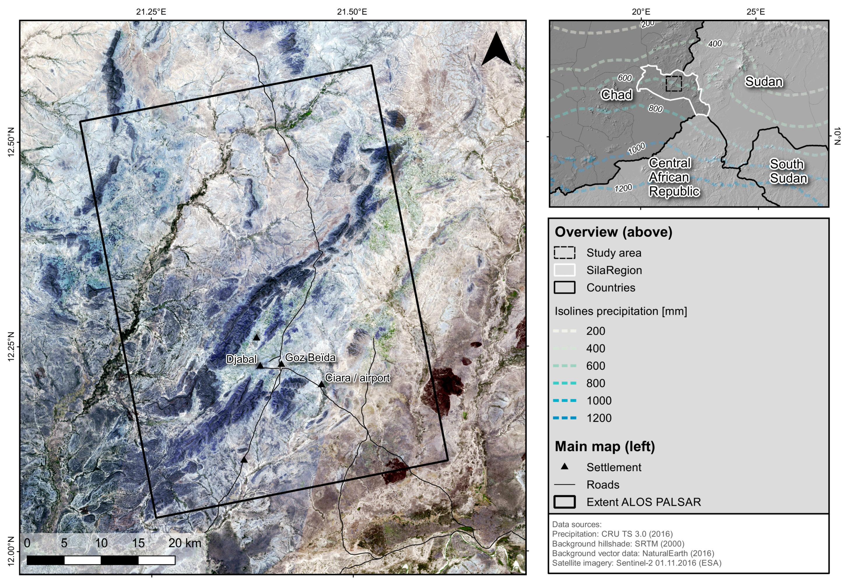
Figure 2.
Identified areas used for the stratified random sampling.

Figure 3.
Calculation of the weighted Natural Resource Depletion Index (NRDw).

Figure 4.
Left: Design of the approach: Each classified image delivers aggregated values of natural resources. Right: Changes between the years are expressed as weighted Natural Resource Depletion (NRDw), demonstrated for the period between 2007 and 2008.
Figure 4.
Left: Design of the approach: Each classified image delivers aggregated values of natural resources. Right: Changes between the years are expressed as weighted Natural Resource Depletion (NRDw), demonstrated for the period between 2007 and 2008.
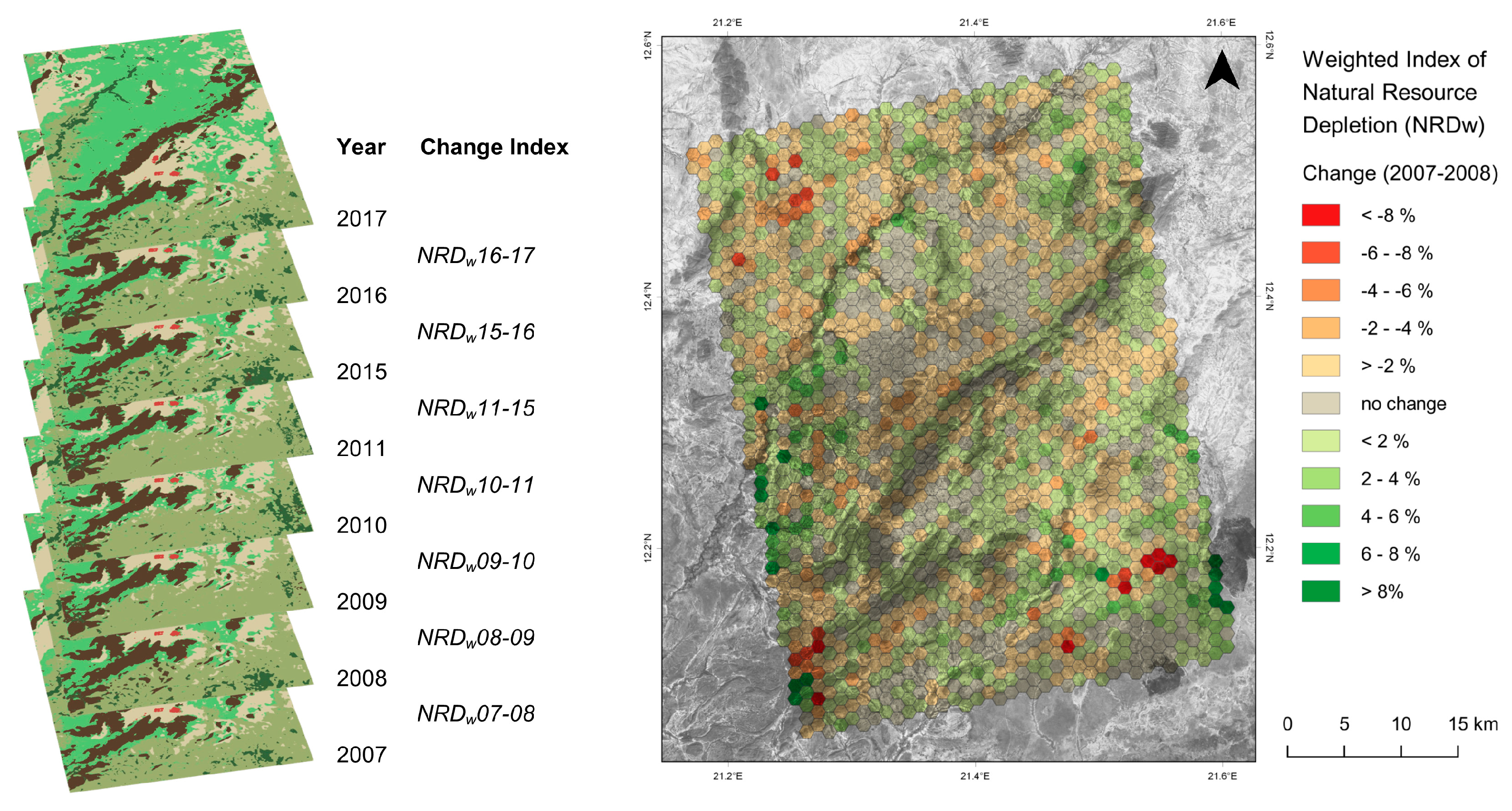
Figure 5.
Calculation of the variability v of an area.

Figure 6.
Weighted Natural Resource Depletion Index (NRDw) for the study area during the investigated period. Note that, due to lack of available L-band SAR data, an annual investigation was not possible between 2011 and 2015.
Figure 6.
Weighted Natural Resource Depletion Index (NRDw) for the study area during the investigated period. Note that, due to lack of available L-band SAR data, an annual investigation was not possible between 2011 and 2015.

Figure 7.
Weighted Natural Resource Depletion Index (NRDw) and variability for the study area between 2007 and 2017.
Figure 7.
Weighted Natural Resource Depletion Index (NRDw) and variability for the study area between 2007 and 2017.

Figure 8.
Frequency distribution of the variability of grid cells within the study area compared to their NRDw index for the time between 2007 and 2017. Note the logarithmic scaling of the y-axis.
Figure 8.
Frequency distribution of the variability of grid cells within the study area compared to their NRDw index for the time between 2007 and 2017. Note the logarithmic scaling of the y-axis.
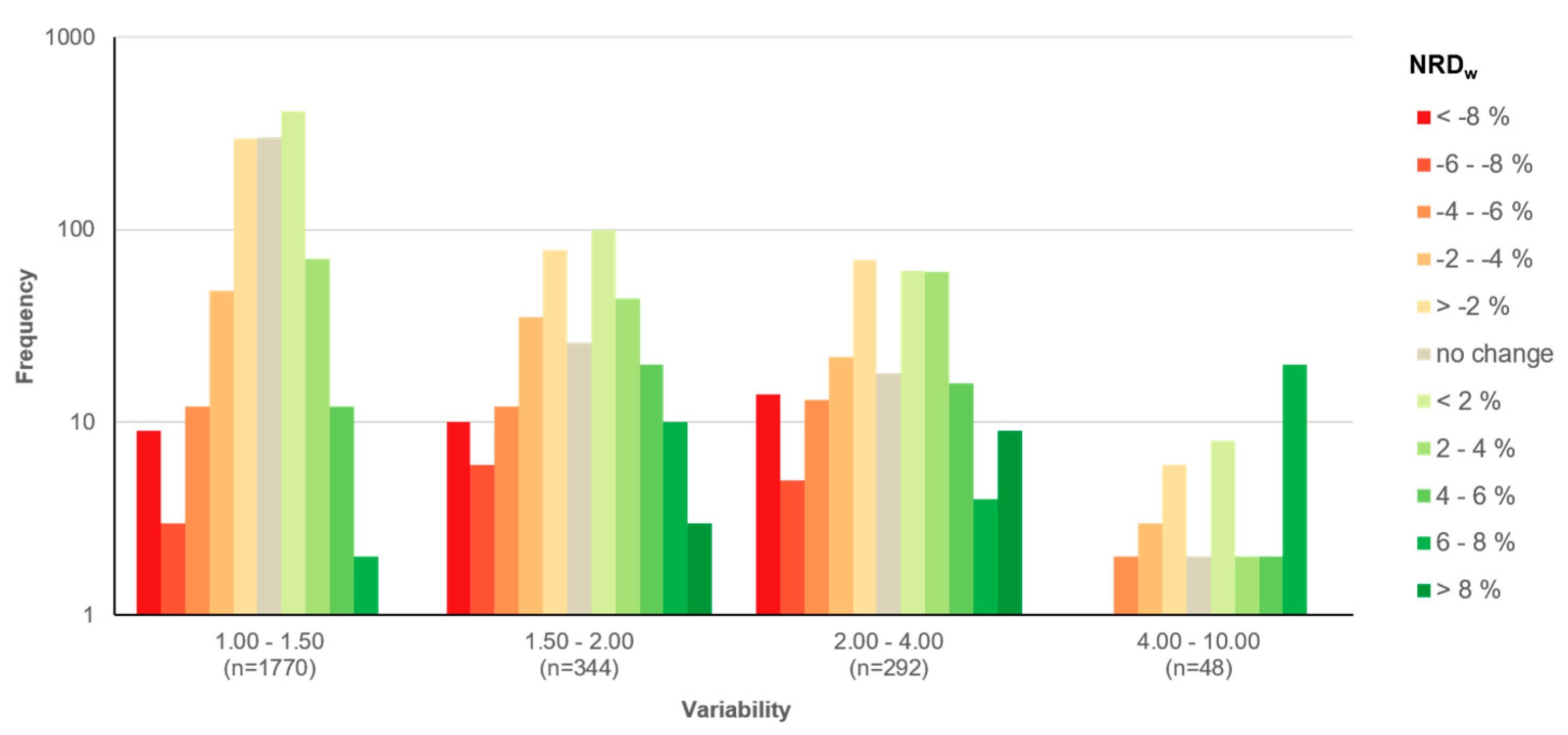
Figure 9.
Monthly precipitation and temperature for the study area.
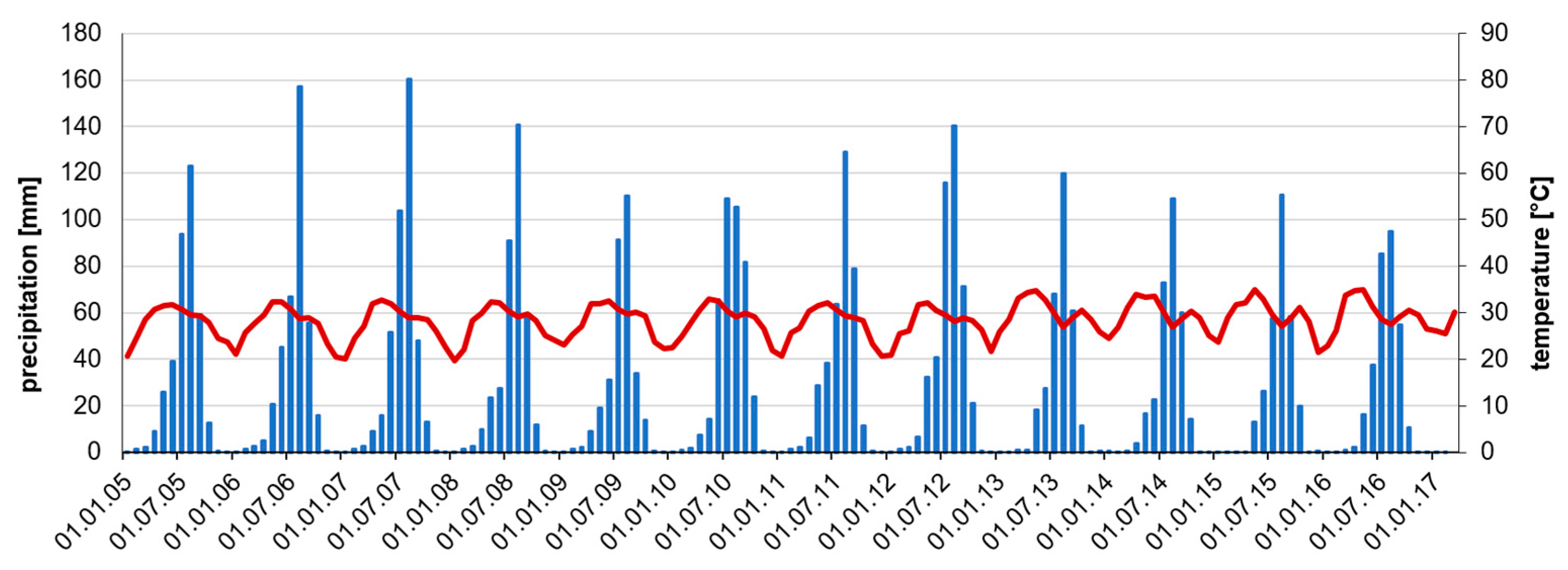

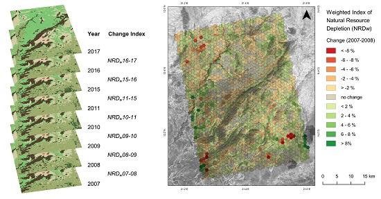
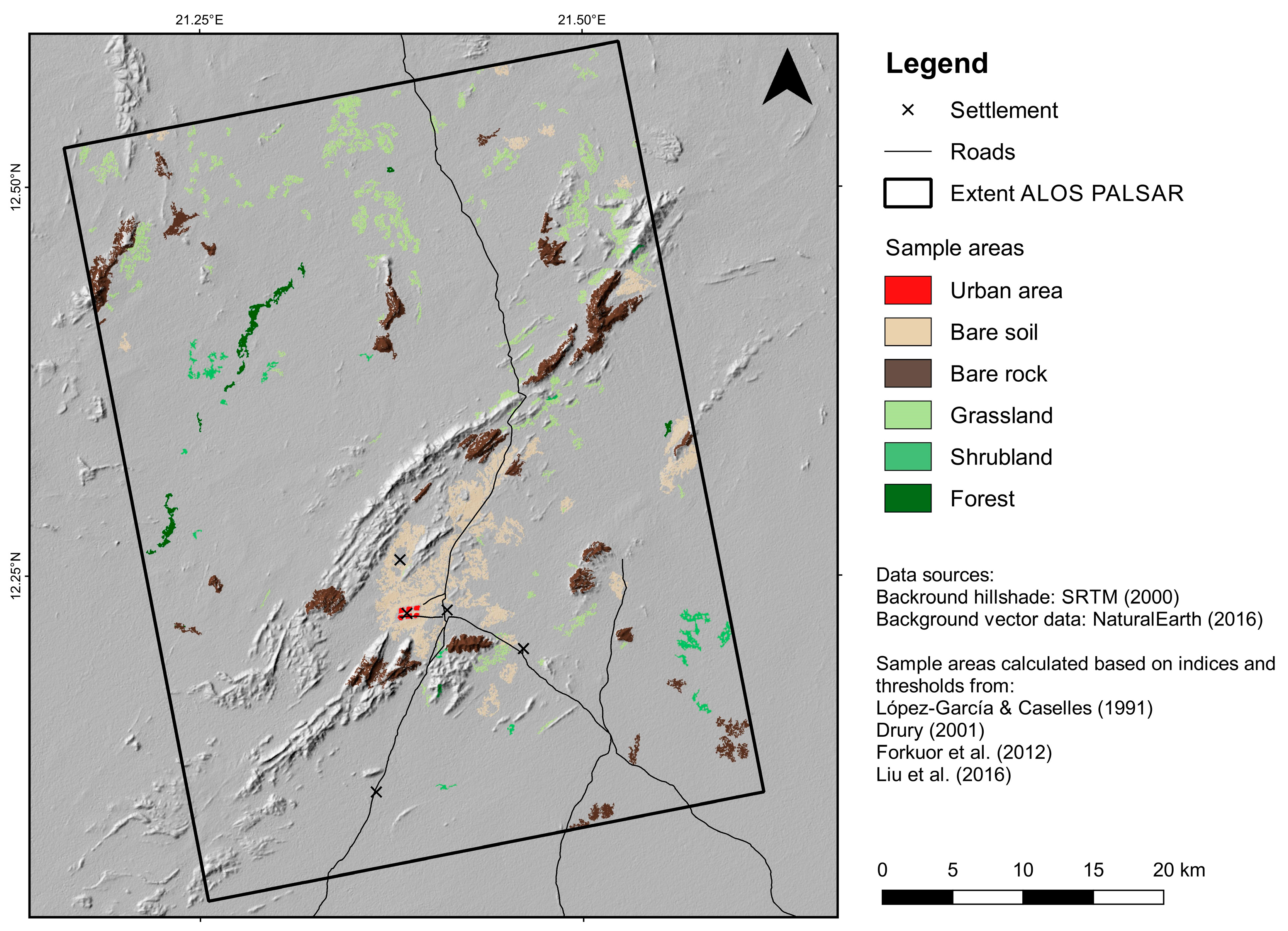
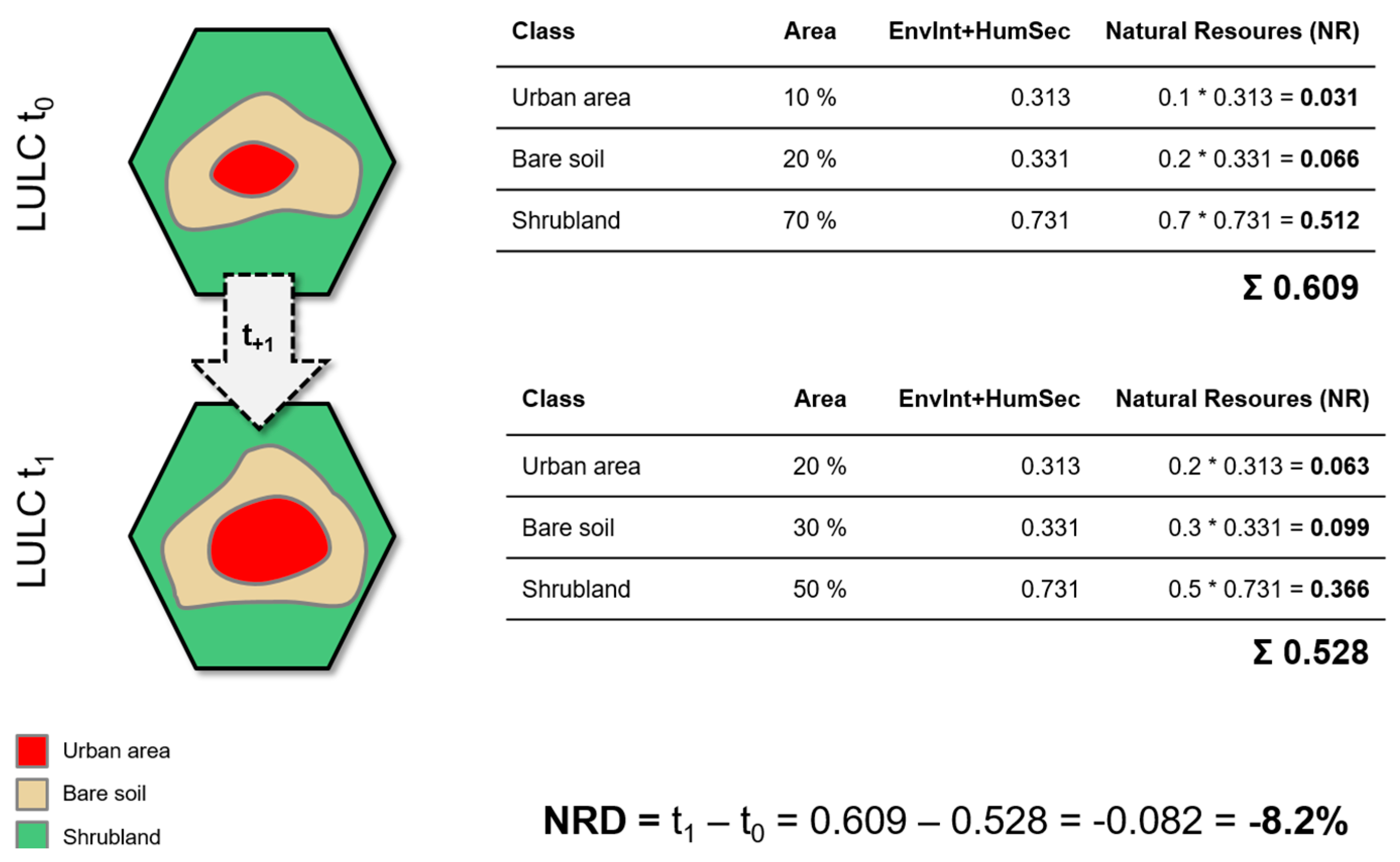
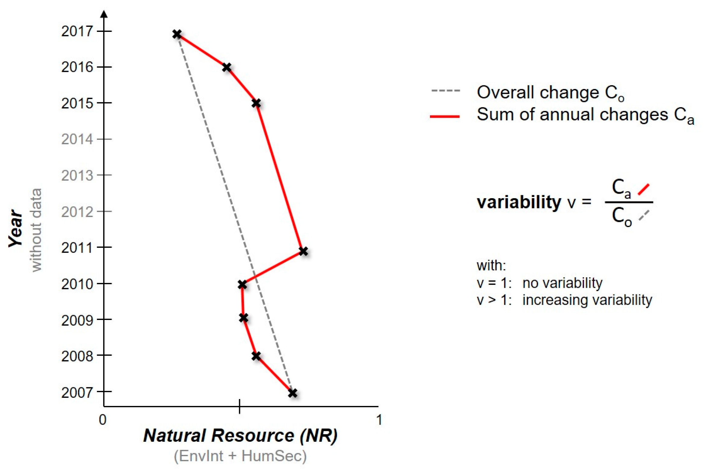
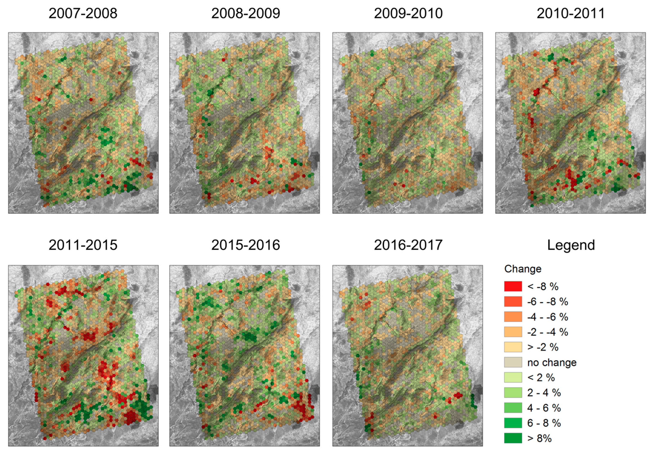
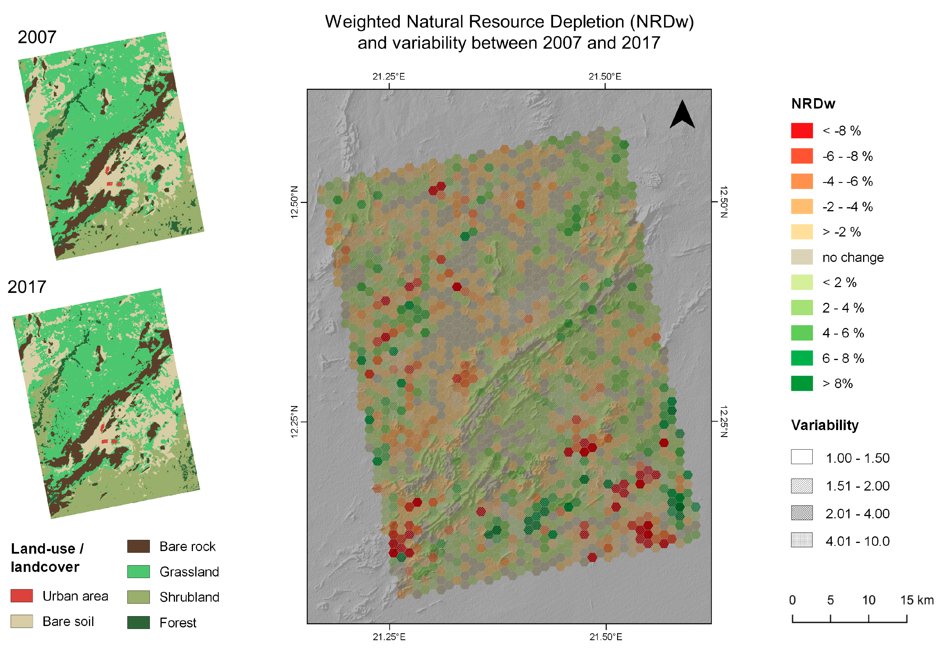
Table 1.
Satellite imagery used in this study.
| Year/Δt | Date | Sensor | Comment |
|---|---|---|---|
| 2007/18 days | 24 December 2006 | ALOS PALSAR | SLC-off |
| 11 January 2007 | Landsat ETM+ | ||
| 2008/2 days | 27 December 2007 | ALOS PALSAR | SLC-off |
| 29 December 2007 | Landsat ETM+ | ||
| 2009/18 days | 29 December 2008 | ALOS PALSAR | SLC-off |
| 16 January 2009 | Landsat ETM+ | ||
| 2010/30 days | 2 December 2009 | Landsat ETM+ | SLC-off |
| 1 January 2010 | ALOS PALSAR | ||
| 2011/20 days | 19 February 2011 | ALOS PALSAR | SLC-off |
| 11 March 2011 | Landsat ETM+ | ||
| 2015/0 days | 23 January 2015 | ALOS-2 | |
| 23 January 2015 | Landsat OLI/TIRS | ||
| 2016/6 days | 22 January 2016 | ALOS-2 | |
| 28 January 2016 | Landsat OLI/TIRS | ||
| 2017/15 days | 2 March 2017 | ALOS-2 | |
| 15 February 2017 | Landsat OLI/TIRS |
Table 2.
Land-use and land cover (LULC) classes and identification of sample areas in the study area.
Table 2.
Land-use and land cover (LULC) classes and identification of sample areas in the study area.
| Class | Samples | Criterion | Source |
|---|---|---|---|
| Urban area | 161 (7.2%) | Area of the camp in 2007 | - |
| Bare soil | 390 (17.6%) | Red < 0.25 & SWIR1 > 0.35 | Drury (2001) [98] |
| Bare rock | 352 (15.9%) | SWIR1/SWIR2 > 1.5 | Drury (2001) [98] |
| Grassland | 374 (15.6%) | NDVI > 0.15 & NDVI < 0.25 | Forkuor et al. (2012) [95] |
| Shrubland | 126 (5.6%) | Red < 0.2 & NIR > 0.3 & SWIR < 0.3 | Liu et al. (2016) [99] |
| Forest | 172 (7.8%) | NDVI > 0.2 | Forkuor et al. (2012) [95] |
| Burnt areas | 0 (0%) | NBR > 0.15 | López-García & Caselles (1991) [97] |
Table 3.
Producer’s accuracy for the texture-based classification of SAR images using the Random Forest classifier.
Table 3.
Producer’s accuracy for the texture-based classification of SAR images using the Random Forest classifier.
| 2007 | 2008 | 2009 | 2010 | 2011 | 2015 | 2016 | 2017 | |
|---|---|---|---|---|---|---|---|---|
| Urban area | 89.3% | 91.3% | 90.7% | 92.0% | 89.3% | 86.0% | 90.7% | 70.53% |
| Bare soil | 92.0% | 90.7% | 92.0% | 93.3% | 92.0% | 89.3% | 86.7% | 77.88% |
| Bare rock | 96.0% | 95.3% | 96.0% | 94.0% | 96.0% | 94.0% | 93.3% | 90.91% |
| Grassland | 83.3% | 80.7% | 88.7% | 83.3% | 82.0% | 94.0% | 76.7% | 82.23% |
| Shrubland | 75.3% | 70.7% | 76.0% | 77.3% | 75.3% | 68.7% | 76.7% | 82.64% |
| Forest | 70.7% | 71.3% | 70.7% | 70.0% | 69.3% | 67.3% | 64.0% | 66.92% |
Table 4.
User’s accuracy for the texture-based classification of SAR images using the Random Forest classifier.
Table 4.
User’s accuracy for the texture-based classification of SAR images using the Random Forest classifier.
| 2007 | 2008 | 2009 | 2010 | 2011 | 2015 | 2016 | 2017 | |
|---|---|---|---|---|---|---|---|---|
| Urban area | 100.0% | 100.0% | 100.0% | 100.0% | 98.5% | 99.2% | 100.0% | 100.0% |
| Bare soil | 82.6% | 84.5% | 84.7% | 85.4% | 82.1% | 76.1% | 79.3% | 82.5% |
| Bare rock | 97.3% | 95.3% | 99.3% | 97.2% | 94.1% | 95.9% | 94.0% | 95.9% |
| Grassland | 63.1% | 61.4% | 64.6% | 62.8% | 64.7% | 57.8% | 59.3% | 57.6% |
| Shrubland | 83.7% | 84.8% | 85.7% | 82.3% | 82.5% | 80.5% | 80.5% | 78.4% |
| Forest | 89.8% | 82.3% | 90.6% | 92.9% | 89.7% | 84.2% | 93.2% | 87.3% |
Table 5.
Importance of the analyzed land-use and land cover classes on environmental integrity (EnvInt) and human security (HumSec) for the calculations of an integrated value of natural resources (NR).
Table 5.
Importance of the analyzed land-use and land cover classes on environmental integrity (EnvInt) and human security (HumSec) for the calculations of an integrated value of natural resources (NR).
| Class | EnvInt 35% | HumSec 65% | NR 100% |
|---|---|---|---|
| Urban area | 0.00 | 0.50 | 0.313 |
| Bare soil | 0.30 | 0.35 | 0.331 |
| Bare rock | 0.20 | 0.25 | 0.231 |
| Grassland | 0.50 | 0.45 | 0.469 |
| Shrubland | 0.70 | 0.75 | 0.731 |
| Forest | 0.95 | 0.90 | 0.919 |
Table 6.
Development of Natural Resources (NR) and weighted Natural Resource Depletion (NRDw).
| 2007 | 2008 | 2009 | 2010 | 2011 | 2015 | 2016 | 2017 | |
|---|---|---|---|---|---|---|---|---|
| NRmax | 91.9% | 91.5% | 90.7% | 90.1% | 91.4% | 91.7% | 89.5% | 88.6% |
| NR95% | 73.5% | 76.2% | 74.7% | 74.3% | 74.6% | 73.9% | 73.1% | 73.3% |
| NRmean | 46.9% | 47.1% | 47.0% | 47.1% | 46.9% | 46.5% | 46.8% | 47.0% |
| NRmedian | 45.7% | 45.4% | 45.9% | 45.9% | 45.8% | 44.3% | 45.6% | 45.1% |
| NR5% | 24.8% | 24.4% | 25.0% | 24.9% | 24.2% | 25.0% | 25.4% | 25.6% |
| NRmin | 23.1% | 23.1% | 23.1% | 23.1% | 23.1% | 23.1% | 23.1% | 23.1% |
| NRsum | 840.8 | 844.6 | 843.5 | 843.8 | 840.7 | 833.1 | 839.9 | 842.8 |
| NRDw mean | 0.187% | −0.037% | 0.016% | −0.175% | −0.421% | 0.379% | 0.158% | |
| NRDw net | 3.36 | −0.65 | 0.28 | −3.14 | −7.55 | 6.79 | 2.83 |
Table 7.
NRDw net values for the investigated time-steps compared to trends in precipitation (Δprec) and temporal baselines of the used SAR images (SAR Δd).
Table 7.
NRDw net values for the investigated time-steps compared to trends in precipitation (Δprec) and temporal baselines of the used SAR images (SAR Δd).
| 2007–2008 | 2008–2009 | 2009–2010 | 2010–2011 | 2011–2015 | 2015–2016 | 2016–2017 | r (NRDw) | |
|---|---|---|---|---|---|---|---|---|
| NRDw net | 3.36 | −0.66 | 0.28 | −3.14 | −7.55 | 6.80 | 2.833 | 1.00 |
| Δprec | −37.7 | −55.7 | 97.7 | −49.9 | −74.6 | 15.8 | - * | 0.47 |
| SAR Δd | 12 | 12 | 18 | 88 | 1078 ** | 8 | 12 | −0.61 |
* Changes in precipitation could not be assessed between 2016 and 2017 as no all-season records were available at the time of the study. ** In order to not distort the statistics, the temporal baseline of four years was excluded from the calculation of r.
© 2017 by the authors. Licensee MDPI, Basel, Switzerland. This article is an open access article distributed under the terms and conditions of the Creative Commons Attribution (CC BY) license (http://creativecommons.org/licenses/by/4.0/).
Share and Cite
MDPI and ACS Style
Braun, A.; Hochschild, V. A SAR-Based Index for Landscape Changes in African Savannas. Remote Sens. 2017, 9, 359. https://doi.org/10.3390/rs9040359
AMA Style
Braun A, Hochschild V. A SAR-Based Index for Landscape Changes in African Savannas. Remote Sensing. 2017; 9(4):359. https://doi.org/10.3390/rs9040359
Chicago/Turabian StyleBraun, Andreas, and Volker Hochschild. 2017. "A SAR-Based Index for Landscape Changes in African Savannas" Remote Sensing 9, no. 4: 359. https://doi.org/10.3390/rs9040359
Note that from the first issue of 2016, this journal uses article numbers instead of page numbers. See further details here.