
The Use of Landscape Metrics and Transfer Learning to Explore Urban Villages in China

1
State Key Laboratory of Information Engineering in Surveying, Mapping and Remote Sensing, Wuhan University, Wuhan 430079, China
2
School of Remote Sensing and Information Engineering, Wuhan University, Wuhan 430079, China
*
Authors to whom correspondence should be addressed.
Remote Sens. 2017, 9(4), 365; https://doi.org/10.3390/rs9040365
Submission received: 4 January 2017
/
Revised: 18 March 2017
/
Accepted: 9 April 2017
/
Published: 13 April 2017
(This article belongs to the Special Issue Earth Observation in Planning for Sustainable Urban Development)
Abstract
:Urban villages (UVs), the main settlements of rural migrant workers and low-income groups in metropolitan areas of China, have become of major concern to city managers and researchers due to the rapid urbanization in recent years. A clear understanding of their evolution and spatial relationships with the city is of great importance to policy formulation, implementation and assessment. In this paper, we propose a new framework based on landscape metrics and transfer learning for the long-term monitoring and analysis of UVs, and we apply it to Shenzhen and Wuhan, two metropolitan cities of China, with high-resolution satellite images acquired from 2003–2012 and 2009–2015, respectively. In the framework, landscape metrics are used for identifying the UVs and quantifying their evolution patterns on the basis of a city-UV-building hierarchical landscape model. Transfer learning is also introduced to use the samples and features across the spatial and temporal domains, which reduces the time and labor cost, as well as improves the mapping accuracies by 3–10%. The results show that the total area of UVs has decreased by less than in Shenzhen and more than in Wuhan. Moreover, we observe significant spatial correlations in the development of UVs in Shenzhen. By contrast, no strong spatial correlations are found in Wuhan’s UVs, indicating that their development is largely independent of the spatial location. The results reveal two typical strategies, i.e., demolition and renovation, towards the redevelopment of UVs in China.
1. Introduction
The developing world is experiencing profound changes caused by urbanization and industrialization. A large amount of people move to cities from the country in search of better work and living. Settlements of low-income people, often without formal citizenship, have arisen in many developing countries with different socioeconomic backgrounds, e.g., slums in India [1] and South Africa [2] and the favelas in Brazil [3], and they mostly feature poor living environments. It has been reported that there is a population of about one billion people living in poor urban regions (e.g., slums) worldwide, most of which are in developing countries [4]. The living conditions in these informal settlements and their impact on urban development and the corresponding strategies have become the focus of city managers and researchers [5,6,7].
In China, one of the largest developing countries, the analog of informal settlements is “urban villages” (UVs), which originate from villages [8,9]. During the rapid urbanization of China, the growing cities have engulfed the farmland of neighboring villages, leaving the rural settlements intact. These settlements are called UVs. Although totally surrounded by newly-urbanized areas, UVs remain independent administrative entities collectively managed by the original villagers. The absence of planning and management has led to disorderly development. UVs have gradually become settlements of migrant workers and low-income groups due to the inexpensive housing, and they have close geographical and socioeconomic relationships with the city. A number of studies have discussed the effect of UVs on urban development from various socioeconomic perspectives [5,10,11,12], e.g., affordable housing for migrants [13], the relationships between UVs and public facilities [14], etc. However, the spatial relationship between UVs and the city and the long-term impact of urban development, as well as government planning on UVs have seldom been studied, especially in a quantitative manner. Good knowledge of the long-term development of UVs will help city planners to make appropriate UV redevelopment policies.
Recently, a few studies of informal settlements in developing countries have used remotely-sensed data, especially very high-resolution (VHR) satellite imagery, as their major data source [1,15,16,17,18,19,20,21,22]. Hofmann et al. [23] used an object-based approach to detect informal settlements in Rio de Janeiro. Owen and Wong [24] proposed to differentiate informal settlements with multiple features, including spectral, texture, geomorphology and road accessibility metrics. In our recent work [14], several scene classification techniques for detecting UVs were compared. Although many features and algorithms have been proposed in previous studies, few of them have been evaluated with a remotely-sensed data time series. As far as UVs are concerned, their evolution patterns have mostly been reported qualitatively in the past. Meanwhile, despite the great potential in long-term urban monitoring [25,26,27,28], remotely-sensed data have seldom been used for analyzing UVs. The role of remote sensing in guiding city and UV development, particularly long-term planning of UVs, needs to be further recognized and advanced.
Specifically, in the use of multi-temporal high-resolution remotely-sensed data for analyzing UV development, there are two major problems to be resolved: (1) how to model a UV. UVs feature a concentration of small and low buildings [29], and the composition and configuration of the land cover (including buildings, vegetation, etc.) is the key to differentiating UVs from other urban areas. However, in most of the previous studies [18,19,23,30,31,32], informal settlements have usually been viewed as pixels or objects (i.e., a collection of adjacent pixels of similar spectral characteristics), which cannot effectively represent the composition and configuration of the land cover in a larger spatial scope. (2) The other is how to make use of the features and samples across the spatial and temporal domains. In general, features and samples derived from one image cannot be applied to other images to identify UVs, because they are image dependent, and image differences resulting from the various sensors, atmospheric conditions and azimuth angles always exist in a long time series [33,34]. However, it is time consuming and labor intensive to identify UVs from each image independently.
Therefore, in this study, we develop a new framework based on landscape metrics and transfer learning for the long-term monitoring and analysis of UVs. Landscape metrics are employed for the identification and characterization of UVs based on a proposed hierarchical landscape model, and transfer learning is introduced to use the features and samples across the spatial and temporal domains. We apply the proposed method to Shenzhen and Wuhan, two metropolitan cities of China, and present the spatiotemporal patterns of UV development. According to our findings, we then discuss the roles and impacts of UVs in urban development and their redevelopment strategies.
2. Study Areas and Data
In this study, we experimented with the urban areas of Wuhan and Shenzhen (Figure 1), two typical cities accompanied with a large number of UVs in recent decades. Wuhan, situated at the confluence of the Yangtze and Han rivers, has been the capital of Hubei province and the largest city in Central China for centuries. It is one of the most populous metropolitan cities in China. Shenzhen is a very young city, which is situated in the Pearl River Delta, one of the most developed areas in China. It became the first Special Economic Zone of China in 1979 and has experienced swift economic development and extraordinary city expansion and population inflow since then [26,35]. The two cities have different socioeconomic backgrounds and urbanization patterns, which also affect the development of UVs.
Multi-temporal high-resolution satellite images were acquired over the main urban areas of Wuhan and Shenzhen (Table 1), which have been radiometrically calibrated. The Wuhan dataset consists of three images from 2009–2015 and covers an area of km. The Shenzhen dataset consists of six images from 2003–2012 and covers an area of km.
3. Methods
We describe the proposed landscape model and corresponding landscape metrics in Section 3.1 and the transfer learning methods in Section 3.2. The complete workflow is presented in Section 3.3.
3.1. City-UV-Building Hierarchical Landscape Model
UVs were originally rural settlements. Engulfed by expanding cities, they no longer neighbor farmland, but instead are surrounded by various urbanized areas, such as commercial areas with skyscrapers and formal residential areas, which constitute the city together with UVs (Figure 2a,c,e). Due to the absence of proper planning and management, UVs mainly feature low and crowded buildings, which were constructed by villagers and are now rented to migrants and low-income groups (Figure 2b,d,f). Accordingly, open space and green land are scarce in UVs compared to other urban areas. Hence, we can identify UVs from high-resolution remote sensing images according to the composition and configuration of the land cover, especially buildings.
For the purpose of identifying UVs and further analyzing their development dynamics, we need to quantify the spatial relationship between the UV and the buildings and the relationship between the city and UVs. According to their relationships described above, we present a hierarchical landscape model consisting of two spatial structures at the city and UV scales, respectively, where the term “landscape” refers to a spatial structure that consists of patches of one or several classes [36]. Specifically, at the city scale, the city is the landscape, and the UVs and other urban areas (e.g., commercial areas) are patches within the city landscape; at the UV scale, the UV is the landscape, buildings, vegetation, etc., are patches within the UV landscape. In this paper, we mostly focus on city-UV and UV-building structures at the two scales.
The structures and spatial patterns of a landscape, including the composition and configuration of the landscape patches, can be quantified by various indices, which are usually called landscape metrics [37,38,39,40,41,42,43]. This paper uses two types of landscape metrics, i.e., patch- and landscape-level metrics [36]. Patch-level metrics are computed for each patch, e.g., the shape index (SHAPE, Table 2) of a building in a UV or the SHAPE of a UV in the city. Landscape-level metrics are computed for the entire landscape and can often be defined based on the corresponding patch-level metrics, e.g., the mean shape index (MSI, Table 3) of buildings in a UV or the MSI of UVs in the city.
To realize the conceptual hierarchical landscape model and apply the landscape metrics in practice, we need to create the corresponding landscapes and patches in the context of remote sensing images. (1) City-UV: The study area is the city landscape. As one of the major products of this study, accurate UV patches are not available before they are identified from remote sensing images. Alternatively, we use the moving window strategy to divide the city landscape into square sub-landscapes, which are hereinafter referred to as “scenes” (Figure 3). The scene size is 120 m, which is empirically chosen (Section 4.1.3). The scenes are then identified as UVs/non-UVs by the composition and configuration of the land cover. For the further landscape pattern analysis, accurate UV patches are created by manually refining the detection results. (2) UV-building: Every UV patch in the city-UV structure can be viewed as the landscape in the UV-building structure. To create building patches for the UV landscape, we employ the morphological building index (MBI) [44,45,46] for unsupervised and rapid extraction from the high-resolution images, which has been used in a number of recent studies including built-up area detection [47] and urban change detection [48]. We also create vegetation patches using the normalized difference vegetation index (NDVI). Since buildings are dominant in UVs, vegetation patches are not used for analyzing the UV landscape, but to help differentiate UV scenes from others (the percentage of UV areas in the city landscape (PLAND), mean patch size (MPS) and patch size standard deviation (PSSD) in Table 3 are computed for the vegetation patches).
Table 2 and Table 3 list the landscape metrics used for the two structures respectively. To characterize the city-UV structure, we select a suite of patch- and landscape-level metrics available in FRAGSTATS software [36], which are detailed in Section 3.3.4. They have previously been used for describing urban land uses and urban growth, assessing urban contiguity and investigating the spatial heterogeneity of different landscapes [38,42,50,51,52]. To identify UV scenes, we propose a collection of 25 metrics. A small number of commonly-used metrics is enough to describe the UV-building structure, but additional metrics could help to better differentiate UV scenes from others. In fact, landscape metrics are mostly used as indicators, and a few studies have used them as features for classification and detection [53]. We select and define these metrics from various views (e.g., area, shape and distance). Some metrics might not help the identification, but this can fortunately be addressed by feature weighting, i.e., the evaluation of the significance of the different metrics (Section 3.2). Some of them are also used to characterize the UV-building structure and are further explained in Section 3.3.4.
3.2. Transfer Learning: Sample and Feature Weighting
To differentiate UV from non-UV scenes, we first quantify the scenes by the various metrics and represent the scenes as one-dimensional vectors by stacking the metric values, and we then classify the vectors. Accordingly, we need a collection of suitable metrics to quantify the scenes and labeled scenes to train the classifier. Although we could manually label scenes from the input image and select suitable metrics (e.g., those listed in Table 3), scenes and metrics that have been evaluated with previous images are preferred, because this not only greatly reduces the time and labor cost, but also enables an efficient and automatic procedure for the monitoring of UVs.
However, the vector (i.e., metric values) associated with the same scene at different times is generally different due to the image differences caused by the various sensors, atmospheric conditions and azimuth angles. For instance, the shape index of building patches in UVs may have different normal distributions, and , in different images. When such labeled vectors derived from previous scenes are used to train the classifier, wrongly-classified scenes will occur due to the difference in the distributions of the metric values between images.
Another problem emerges when we apply metrics that have been proven to be suitable for one city to other cities. Although the main characteristics of UVs are the same across cities, there are always some different aspects in their composition or configuration. For instance, the UVs in Shenzhen usually have narrower spaces between buildings than in Wuhan because of the higher population density [54]. Consequently, discriminative metrics, especially those with specific parameters (e.g., core area metrics), for one city may be ineffective for others, leading to more computation time and inferior detection results.
To address the above two problems, transfer learning, which is attracting increasing interest in remotely-sensed data classification [31,55,56,57,58], is introduced. Transfer learning aims to extract the knowledge from one or more source tasks and applies the knowledge to a target task [59]. In this study, a “task” refers to the identification of UVs from an image using suitable features (i.e., landscape metrics) and labeled samples (i.e., scenes). Then, the completed task with previous images is a source task, whose context (including the identified scenes, the collection of metrics used and the distribution of calculated metric values) is called the source domain. Correspondingly, identifying UVs from a new image is the target task, whose context is called the target domain.
For the first problem, i.e., how to use source domain samples (i.e., scenes) in the target domain, a recently proposed method called the two-stage weighting framework for domain adaption (2SW-MDA) [60] is used in this study. The method assigns different weights to the source domain samples, i.e., sample weighting, which are used to train the classifier in the target domain. Samples with larger weights are considered more important in the training, by which the differences between the distributions of metric values in the source and target domains are minimized in the classification.
To address the second problem, i.e., how to transfer metrics between cities efficiently, we propose a metric propagation and selection procedure. The collection of metrics is first enlarged to enhance the generalization ability for the new city by adding new metrics or replicating existing metrics with different parameters and then reduced by getting rid of the insignificant or negative metrics. To evaluate the significance of the metrics, two feature weighting strategies are used: the mean decrease in the Gini index (MDG) [61,62] and the vector angle (VA) (see the Appendix). MDG has been used for the feature selection and assessment of variables [63,64], and VA indicates the contribution of a metric to the transferability of scenes across domains. In contrast with VA, MDG can be computed with less a priori knowledge, but it does not take domain differences into account. We use both of them to fully evaluate the significance of the metrics.
3.3. Processing Chain
The proposed method includes four parts, which are described successively. All analysis were conducted using MATLAB unless specified otherwise.
3.3.1. Preprocessing and Feature Extraction
First, the MBI and the NDVI are computed to extract buildings and vegetation from remote sensing images (Section 3.1), where radiometric calibration is required because the NDVI is a spectral index. In this study, all images (Table 1) were acquired with radiometric and geometric calibration in advance.
3.3.2. Sample and Metric Preparation
Second, images are divided into half-overlapped scenes (Figure 3). The scene size is determined according to the common scale of UVs, which is 120 m in this study (Section 4.1.3). Then, the labeled samples (i.e., scenes) and the collection of metrics used to quantify the UV-building landscape are either selected manually or acquired from previous tasks.
In this study, we selected 12 labeled samples, including six UV and six non-UV scenes, for the Shenzhen dataset, which have the same locations in different images. They were used as training samples in the classification. Therefore, we classified an image with labeled samples from earlier images (i.e., source domains). For example, the Shenzhen 2007 QuickBird image was classified using labeled samples from earlier Shenzhen 2003 and 2005 QuickBird images. Since Wuhan images were acquired later, we also used earlier Shenzhen-labeled samples as their training samples with the help of sample weighting (Section 3.2). For example, the Wuhan 2009 GeoEye-1 image was classified using labeled samples from Shenzhen 2003–2007 QuickBird images.
In terms of metrics, we selected 25 metrics with appropriate parameters (Table 3) for the Shenzhen dataset. Then, we transferred them to the Wuhan dataset by the metric propagation and selection procedure. Specifically, in the experiments, we replicated metrics by changing the parameters, which improves the generalization of metrics for other cities. For example, the buffer width of core area metrics was three pixels for Shenzhen, and for Wuhan, we added core area metrics with five and seven pixels as the buffer width. We then used the propagated collection of metrics for the classification and obtained the metric significance by feature weighting (Section 3.2). Next, the propagated collection was reduced according to the significance, where the number of metrics in the reduced collection was equal to that in the original collection.
3.3.3. Scene Representation and Classification
For each scene, building and vegetation patches are created with the MBI and the NDVI, and the landscape structure is quantified by the selected metrics using FRAGSTATS [36]. The scene is then represented as a vector by stacking the calculated metric values. Finally, using the selected training samples, UV and non-UV scenes are differentiated by classification of the associated vectors: (1) when the training samples are all from the target domain, we just need an ordinary supervised classification; (2) when some of training samples are from source domains, transfer learning is needed.
In this study, for the first case, the random forest (RF) classifier was used because of its high efficiency and accuracy [65]; for the second case, we implemented the sample weighting with 2SW-MDA and employed the support vector machine (SVM) classifier [66] for classification, which allows an explicit use of sample weights in building the classification model, since the RF classifier cannot explicitly take sample weights into account. The RBF kernel was used for SVM, and the parameters of both classifiers were selected by leave-one-out cross-validation.
To evaluate the effectiveness of the proposed method, we needed test samples for a quantitative accuracy assessment. For each image, we used all of the scenes where the UVs occupied more than 90% as positive test samples, whose number ranged from about 90–190 for different images; we used 600 random pure non-UV scenes as negative test samples, which outnumbered the positive samples because of the large proportion of non-UVs in the whole landscape. The Kappa coefficient and omission/commission errors were computed for the assessment.
3.3.4. Post-Processing and Spatial-Temporal Analysis
For accurate landscape analysis of UVs, the raw classification results were further checked and improved manually by removing false detection, refining UV boundaries, etc. Because of the low omission and commission errors (Table 4), the manual refinement did not cost much time.
Then metrics in Table 2 and Table 3 were selected to analyze the city-UV and UV-building structures. To avoid any confusion, subscripts u and b are added to city-UV- and UV-building-related metrics, respectively. Specifically, five patch-level metrics (i.e., AREA, PERIM, SHAPE, CONTIG and NND) and five landscape-level metrics (i.e., CA, PLAND, NP, AWMSI and AWNND) were used for the city-UV structure (Table 2), and for the UV-building structure, six landscape-level metrics with practical meanings were selected from Table 3 according to the metric significance (Section 4.1.4): NP, PLAND, ED, NCA, MNN and MPAR. All metrics used in the landscape analysis were categorized into two groups.
(I) Describing a single UV (11 metrics): AREA and PERIM are the area and perimeter of a UV; SHAPE and CONTIG describe the shape complexity and the connectedness of a UV; NND is the distance of a UV to the nearest neighbor; these five metrics are formulated in Table 2. Another six metrics are related to the inner built-up development of a UV (i.e., the UV-building structure, Table 3): PLAND is the percentage of buildings; NP and NCA are the number of buildings and large buildings in a UV, respectively; ED is the total length of building boundaries per hectare; MNN is the average distance of buildings to their nearest neighbors; and MPAR is the average width-to-length ratio of buildings. Because the building patches obtained by the MBI might be inconsistent across domains because of image differences (e.g., the offset of roofs and shadows), we applied linear regression to the values of the six metrics according to the ground truth.
Moreover, to investigate whether the characteristics and development of the UVs are spatially related, we computed the global and the local Moran’s I [67] using GeoDa [68]. The global Moran’s I is a single value ranging from –1 that measures some specific pattern occurring over the entire area, and the local Moran’s I measures the local spatial association for each UV.
(II) Describing the global patterns of UVs in the city landscape (six metrics): CA and NP are the total area and the number of UVs respectively; PLAND is the percentage of UVs in the whole landscape; these three metrics can monitor the expansion or retraction of UVs. Another three metrics, AWMSI, AWNND and PLAND_AM, are the area-weighted average of SHAPE, NND and PLAND in Group I, respectively, where PLAND_AM can indicate the inner built-up development of UVs at the city scale.
The two groups of metrics were applied to the city-UV-building landscape model established with Shenzhen 2003, 2005, 2007 QuickBird images and 2010, 2012 WorldView-2 images, as well as Wuhan 2009, 2012 GeoEye-1 images and the 2015 WorldView-2 image. The 2010 QuickBird image in the Shenzhen dataset was not used because it was acquired in the same year as the 2010 WorldView-2 image, but with a lower resolution.
4. Results
4.1. Multi-Temporal Mapping of UVs
We applied the proposed method to all images, and Figure 4 shows the raw classification results and the multi-temporal extent of the UVs for Shenzhen and Wuhan, where the extent of UVs has been manually refined based on multiple groups of classification results. Because we used half-overlapped scenes as classification units, the resolution of raw classification results is 60 m, half of the scene size (Figure 3). The main changed areas are shown in rectangles. The UVs showed a large reduction in area in Wuhan from 2009–2015, while the change in Shenzhen is relatively small. A further quantitative analysis of the UVs can be found in Section 4.2.
4.1.1. Effect of Training Samples on the Result
For investigating to what degree samples from source domains are qualified as training samples, the Shenzhen images were reclassified using labeled samples from: (1) the target domain; (2) the source domains without sample weighting; and (3) the source domains with sample weighting (i.e., the proposed method). For each image, the source domains refer to earlier images. For instance, the Shenzhen 2010 QuickBird image has three source domains: Shenzhen 2003, 2005 and 2007 QuickBird images.
The average accuracies produced for each Shenzhen image are shown in Table 4, where the Shenzhen 2003 QuickBird image was excluded from the classification because it had no source domains. Unsurprisingly, classification using the labeled samples from source domains without sample weighting produced the worst results, leading to large omission error up to 0.308. The proposed method yielded the best results with a good trade-off between omission and commission errors, and classification using labeled samples from the target domain (i.e., the common approach) also yielded satisfactory results.
In Table 4, samples from the source and target domains were separately used in the classification. To investigate whether the result could be improved further by using samples from both the source and target domains, we classified the Shenzhen images with four different settings: (1) using source domain samples without sample weighting; (2) using all samples (target domain samples included) without sample weighting; (3) using source domain samples with sample weighting; and (4) using all samples with sample weighting. Results show that including target domain samples improve the accuracies significantly when sample weighting was not conducted (i.e., first two columns of each image in Figure 5), but did not lead to the same accuracy improvement when sample weighting was conducted (i.e., last two columns of each image in Figure 5).
4.1.2. Effect of Feature Weighting on the Result
To evaluate feature weighting in the transfer of metrics across cities, we classified the Wuhan images with different training samples and metrics (Table 5). It can be seen that the use of the Shenzhen samples improves the results greatly. In addition, the proposed metric propagation and selection procedure produces higher accuracies for two out of three images than the original collection in Table 3. Especially, the propagated collection performs the best, but the gaps between the Kappa values produced by the different collections are narrow. For instance, the maximum accuracy difference between the propagated collection and the reduced one by MDG is 0.14.
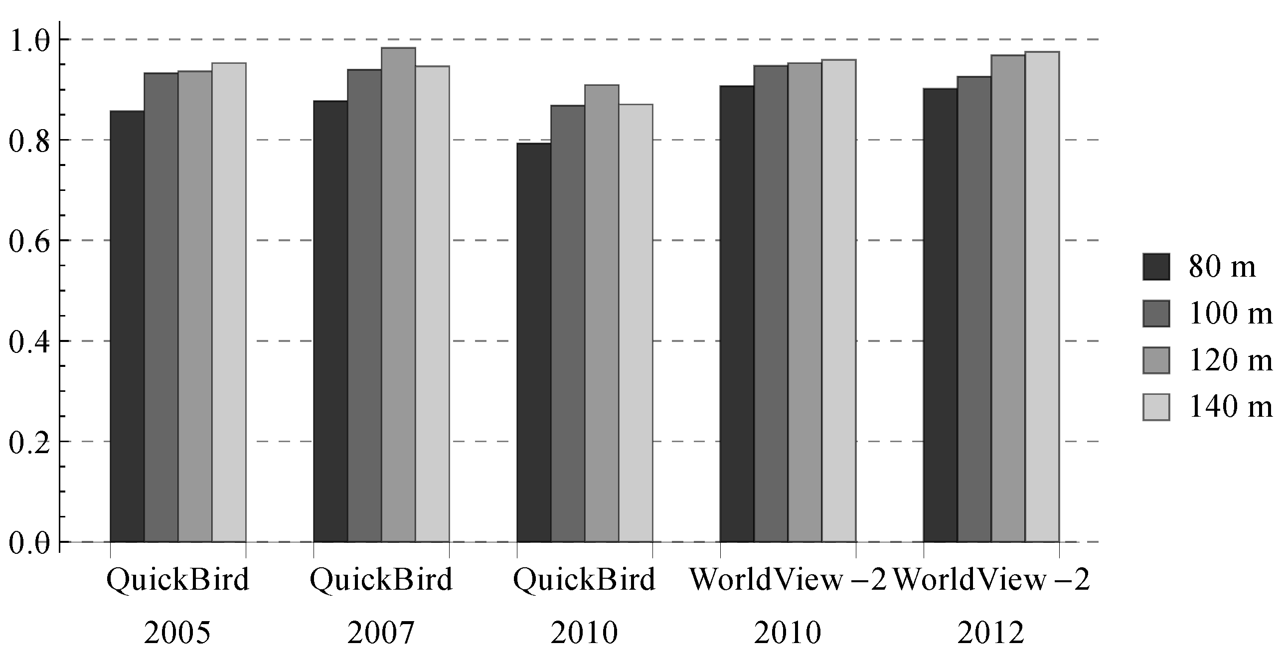
4.1.3. Effect of the Scene Size on the Result
The scene size used in the above experiments was fixed, i.e., 120 m. Because UVs have different sizes and shapes, the scene size does affect the results. To evaluate the effect quantitatively, we classified the Shenzhen images with three other scene sizes, i.e., 80 m, 100 m and 140 m. In the experiments, the training samples were not changed because the metrics used for classification (Table 3) were unrelated to the scene size, i.e., a metric value computed for a UV scene of 80 m was comparable to that computed for a UV scene of 140 m (there were actually two exceptions, i.e., number of patches (NP) and number of core areas (NCA), and we normalized their values according to the scene size). Meanwhile, the sizes of the original test samples (i.e., scenes) were changed from 120 m to 80 m, 100 m and 140 m accordingly, and their center positions were kept unchanged. According to our selection criterion, the test samples were pure scenes at 120 m, and their labels should remain consistent from 80 m–140 m.
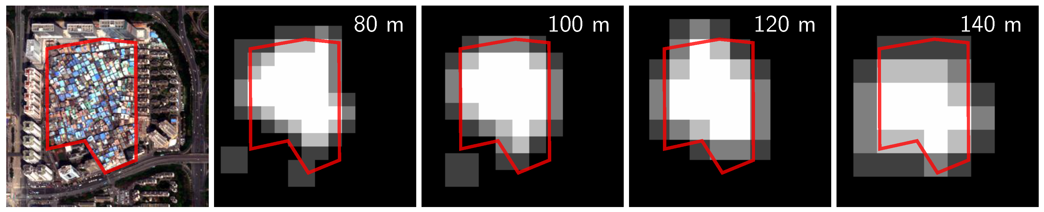
The results show that the accuracies consistently increase as the scene size is increased from 80 m–120 m (Figure 6). When the scene size becomes larger (i.e., 140 m), the accuracies fall for two images and increase slightly for the others. Figure 7 shows the change of the classification results along with the scene size for a Shenzhen UV. The results look finer with a smaller scene size, but there are one or two wrongly-classified scenes in the bottom left corner when the scene size is smaller than 120 m.
4.1.4. Significance of the Landscape Metrics
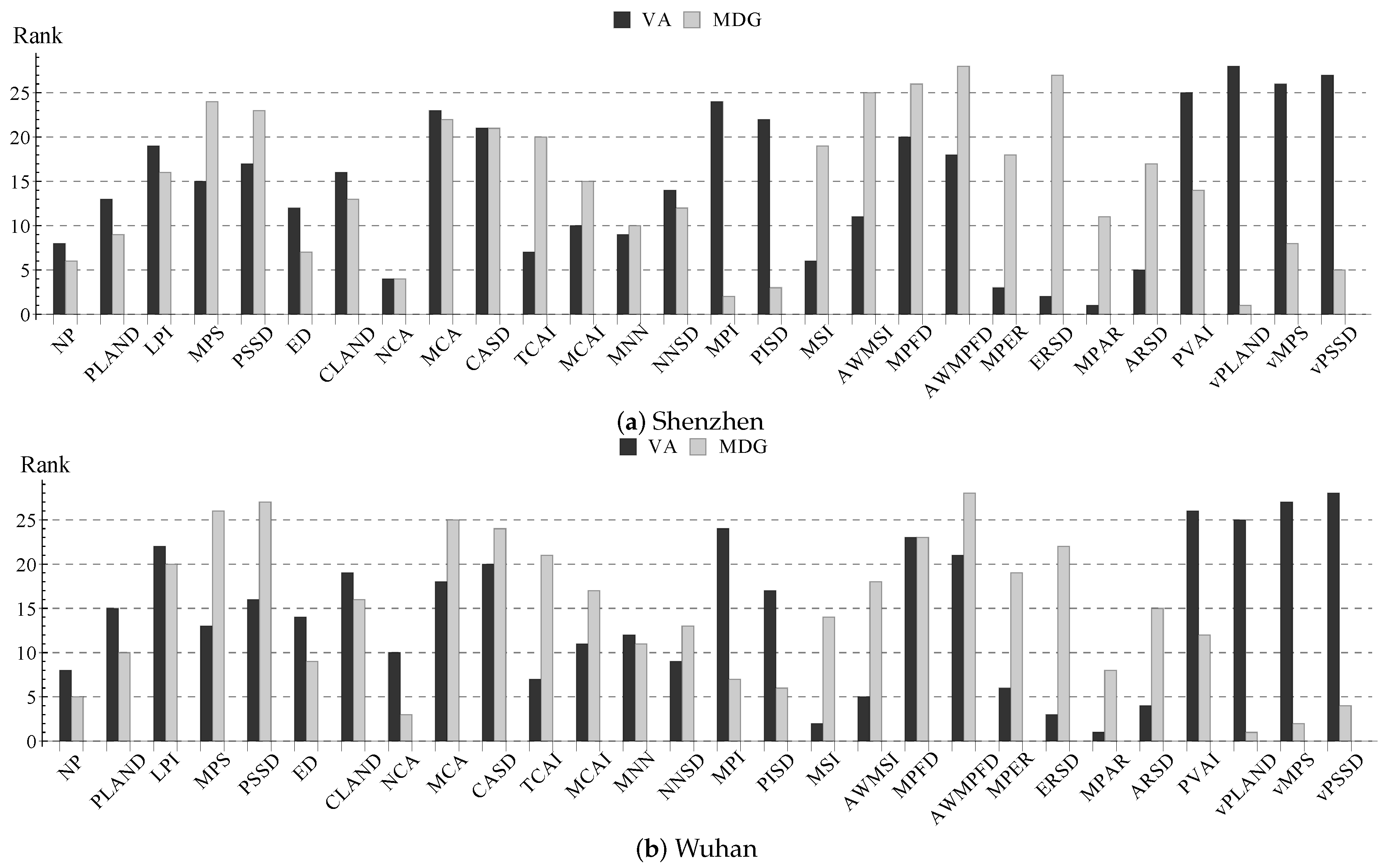
We computed the metric significance with the proposed method (Section 3.2) and converted the numeric values to ordinal numbers, i.e., the ranks of metric significance, where a metric of rank #1 means it is most significant among all metrics in the classification according to the measure (MDG or VA) used. Metrics with the same definition but different parameters were merged, and we finally had 25 metrics related to building patches and three metrics related to vegetation patches (i.e., vPLAND, vMPS and vPSSD).
The metric ranks are similar between Shenzhen and Wuhan, while there are obvious differences between MDG and VA (Figure 8) due to different ideas behind the two measures. In fact, the ranks mostly differ for the metrics related to the building shape (e.g., MSI, extent ratio standard deviation (ERSD) and aspect ratio standard deviation (ARSD)) and vegetation (e.g., vPLAND), which are respectively considered important by VA and MDG. For analyzing the UV-building structure, we selected six metrics according to the metric significance: NP, PLAND, edge density (ED), NCA, mean nearest-neighbor distance (MNN) and mean patch aspect ratio (MPAR) (Section 3.3.4), all of which have practical meanings and rank in the first half for both MDG and VA.
4.2. Spatiotemporal Statistics and Analysis of UVs
4.2.1. Multi-Temporal Patterns of UVs
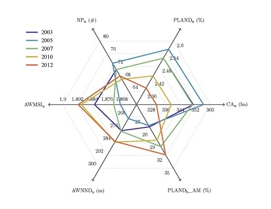
Figure 9 illustrates the evolution of UVs at the city scale with metrics in Group II (Section 3.3.4). On the one hand, a similar trend can be observed for the two cities, i.e., a shift of the ring from upper right to lower left, which is mainly caused by the decreasing area (i.e., CA) and number (i.e., NP) of UVs and the increasing distance between UVs (i.e., AWNND) in the whole city. On the other hand, there are two noteworthy differences between Shenzhen and Wuhan. Firstly, the UVs in Wuhan experienced a more radical demolition program than in Shenzhen. About half of the UVs were demolished in Wuhan study area from 2009–2015, while less than 6% of the UVs in Shenzhen were demolished from 2003–2012. Secondly, the inner built-up development of UVs (i.e., PLAND_AM) in Wuhan decreases consistently with their total area and number, while this is the opposite in Shenzhen. The reasons behind the city-level changes are discussed in Section 5.2.
The distributions of metrics at the UV scale (i.e., Group I in Section 3.3.4) are shown in Figure 10. All aspects of the UVs in two cities have a considerable overlap, indicating the similarity of the UVs between cities. On average, the UVs have a larger area (AREA) and building coverage rate (PLAND) in Shenzhen and a larger neighboring building distance (MNN) in Wuhan. In addition, some opposite trends are found. For instance, the number of large buildings (NCA) is decreasing in Wuhan’s UVs while it is increasing slightly in Shenzhen’s UVs.
4.2.2. Spatial Patterns of UVs
Using the global Moran’s I (Section 3.3.4), we found significant spatial auto-correlation of some metrics, which are mainly related to the UV-building structure (Table 6). In Shenzhen, PLAND, ED, NCA and MNN show a significant positive spatial auto-correlation, i.e., if a UV has a high/low built-up intensity, its neighbors also tend to have a high/low built-up intensity. In Wuhan, such consistent global spatial auto-correlation is not observed.
To further investigate the local spatial patterns, we applied the local Moran’s I to the metrics. In Shenzhen, except the four metrics showing significant spatial auto-correlation, we found CONTIG also had local spatial associations. Figure 11 shows the spatial clusters produced by PLAND, MNN and CONTIG from 2003–2012. In all 15 results, we can clearly see two groups of UVs showing significant spatial correlation: one group at the southwest and the other at the northeast. The former group have a higher building coverage rate (PLAND), a higher connectedness (CONTIG) and a lower neighboring building distance (MNN); UVs in this group are positively correlated. By comparison, UVs in the latter group are diverse, i.e., they have a negative spatial correlation, in terms of connectedness (CONTIG) and neighboring building distance (MNN). In Wuhan, again, no significant local spatial associations were found with any metric, implying that the inner built-up development of UVs in Wuhan is largely independent of UVs’ spatial location.
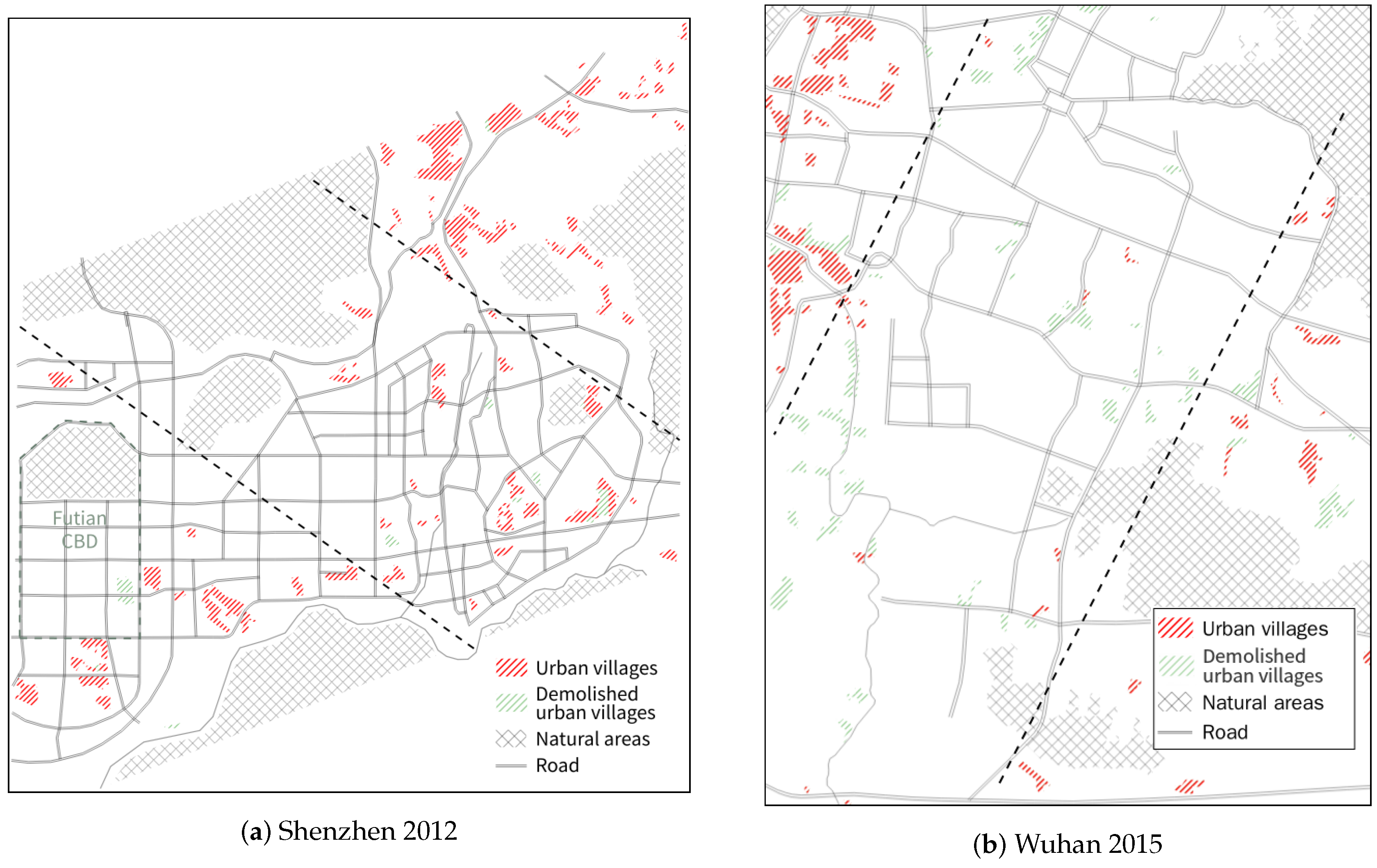
To better illustrate how the global trend and the inner built-up development of UVs are related to the city environment, we present a sketch of the UVs and the main geographical features of each city in Figure 12. UVs that have been demolished are colored in green. Two auxiliary parallel lines are added on each figure according to the foregoing analysis and divide each area into three parts. In Shenzhen, the geographical distance to the city center, Futian central business district (CBD), has significant correlations with the development of UVs: (1) UVs in the south and the center have a higher possibility of being demolished; (2) the building coverage rate (PLAND) of UVs in the south is the highest and becomes consistent spatially from 2003–2012 (Figure 11a); (3) UVs in the north have a building coverage rate lower than the average, and they show heterogeneity in other aspects, such as shape (CONTIG) and neighboring building distance (MNN); (4) UVs in the center are the most heterogeneous, i.e., their shape and inner built-up development are diverse and have no local spatial correlations. In Wuhan, by contrast, the spatial locations of UVs have few correlations with their inner built-up development. Meanwhile, the location of a UV is highly related to whether it should be demolished. In the center, UVs have been basically eliminated, while in other areas, UVs still exist, especially in the west close to the Yangtze River (the natural area at the north west corner of Figure 12b and the blue line in Figure 1c).
5. Discussion
5.1. Monitoring UVs Using a Remotely-Sensed Data Time Series
Compared with time- and labor-intensive field surveys, the proposed framework enables efficient monitoring and assessment of UVs based on a remotely-sensed data time series, providing up-to-date information for city planners, e.g., fast detection of UV-like settlements and quick assessment of redevelopment policies of UVs. Actually, remotely-sensed data have long been acknowledged as an important data source for analyzing the urban environment [27,51,69], and a number of approaches have been proposed for mapping various types of settlements [1,2,3], but the development of UVs in China has seldom been reported or analyzed in the literature. This study fills the gap with a new framework, which differs from the previous studies about informal settlement mapping in three main aspects.
(1) The scene, or the moving window, is used as the classification unit. At a very high spatial resolution (2/2.4 m in this study), UVs are actually a collection of pixels or primitive objects (Figure 2) where the pixels and objects have different categories and physical characteristics. Therefore, it is convenient to identify UVs at a spatial level higher than pixels and primitive objects (e.g., buildings) [23,24]. One popular way is the object-based approach where an image is segmented at multiple levels [16,23,70]. However, the segmentation of a urban environment is still complex and challenging [71,72,73], and we may need to manually edit the segmentation results in the early stage without enough information about UVs. Therefore, the more automatic moving window strategy is adopted in our framework (Figure 3), where the scenes are half-overlapped to increase the mapping accuracy. The only parameter (i.e., the scene size) has been proven to be effective over a wide range (Figure 6).
(2) Landscape metrics are used as features to directly distinguish different urban structures. Previously, only a few studies have used landscape metrics for classification or detection of land cover use [21,53,74], because it is difficult to establish an appropriate landscape model. In this study, based on building and vegetation detection results obtained by the MBI [45,46] and the NDVI, we are able to do this. Compared to the traditional spatial or textural features [75,76], landscape metrics describe the composition and configuration of the land cover in the scene directly. Their definitions are straightforward and mostly parameter-free (Table 3) and, hence, unrelated to the scene size, which greatly reduces the complexity of the feature representation and transfer.
(3) Transfer learning is introduced to reuse samples and features. Transfer learning is attracting increasing interest in the remote sensing community [55,56,57,58] because it can reduce time and labor costs by using previous knowledge, but to date, it has not been used for the long-term monitoring of settlements. The proposed method achieves the reuse of samples and metrics to identify UVs in new images, enabling efficient processing of images without loss of mapping accuracy (Table 4 and Table 5). Thanks to the transfer learning, our method could be easily applied to other metropolitan areas and new booming cities.
In terms of results, the accuracy of the Wuhan dataset (Table 5) is significantly lower than that of Shenzhen (Table 4). Although the accuracies of different cities are actually not comparable because there are many uncontrollable factors (e.g. testing samples), a visual inspection of Figure 4 still indicates that the results of Wuhan are inferior to those of Shenzhen. On the one hand, the accuracy difference can be explained by the differences between the UVs of two cities. Because of the higher population density of Shenzhen [54] and the large-scale demolition of UVs in Wuhan (Figure 4), the building density of UVs in Shenzhen is generally higher. It is therefore easier to identify the UVs in Shenzhen, resulting in a higher accuracy. On the other hand, the metrics in Table 3 were initially collected and evaluated for Shenzhen, and they may not be very appropriate for Wuhan, so a better transfer method for the metrics may be developed.
In fact, owing to the spatiotemporal diversity of UVs and the simplicity of metrics in characterizing landscape structures, existing landscape metrics may be insufficient for certain objects, and new metrics need to be developed accordingly. For instance, several metrics (e.g., MPER and MPAR) in Table 3 are specifically designed for characterizing the spatial composition and configuration of buildings. In addition, features other than landscape metrics could also be integrated into the proposed framework. However, the collection of metrics presented in Table 3 should be a good starting point for similar research.
Because remotely-sensed data only capture physical characteristics, the resulting extent of UVs may not be the same as that recognized by the authorities who also take other factors (e.g., land ownership) into account. In fact, there may be two inconsistent cases. The first case is the areas recognized as UVs by the government, but not in this study. Such areas are mostly rural settlements that are surrounded by urbanized areas, but have not been developed yet at the time the remote sensing images were acquired, which should be identified with later images once they become common UVs with high building and population densities. For example, the increase of UVs in Shenzhen from 2003–2005, which all appear in the north cluster in Figure 12a, actually indicates the transition of original rural settlements to UVs [5]. The second case is the areas identified as UVs in this study, but not by the government. Such areas are mostly degraded or outdated residential areas [77], which often appear in cities (e.g. Wuhan) with many built-up areas of several decades. Because these areas do not originate from villages but have similar physical appearances and function to UVs, the government generally applies the same policies and planning (i.e., demolition and renovation) [78]. Thus, it is important and reasonable to consider such settlements together with UVs in our analysis.
5.2. Development of UVs and the Future
Our research connects the development of UVs with that of the city and buildings from the spatial point of view, and the analysis results at the city scale are basically consistent with government planning, which aims to eliminate UVs finally. In Shenzhen, for instance, owing to “The Master Plan of Urban Village Redevelopment (2005–2010)” and “The Special Plan of City Renewal (`Redevelopment of Old City’) (2010–2015)” proposed by the government, the total area of UVs reached a peak in 2005 and has since fallen (Figure 9a). Similarly, UVs have greatly decreased in area in Wuhan (Figure 9b), where the government has announced plans to demolish all UVs near the city center. In summary, at the city scale, the change of the UVs in Shenzhen is very small, compared to the large-scale demolition in Wuhan (Figure 12). At the UV scale, however, some valuable facts are revealed, not only the quantitative assessment of UV development, but also the city-related spatiotemporal changes. By 2012, as shown in Figure 11, the UVs in Shenzhen had formed three spatial clusters, which are closely related to the distance to the city center (i.e., the Futian CBD). By contrast, no significant spatial relationships were found in Wuhan. In fact, the steady and controllable UV changes occurring in Shenzhen from 2003–2012 reflect the important role the government plays in urban planning, which restrains disordered development of UVs driven by economic interests [9,79].
China is a very large developing country with a remarkable diversity of regional development [80]. The large-scale development of UVs and the resulting severe problems (e.g., public health and security due to poor living environment [29]) is mainly occurring in a few mega cities, including Shenzhen [81], Wuhan [82], Beijing [27], Shanghai [83], etc. For these cities, as indicated in the aforementioned analysis, there are two different strategies towards the redevelopment of UVs. The first strategy is demolition, which is adopted by the majority of cities (e.g., Wuhan) [13,84]. By compensating the villagers who own the land, the government takes over the land ownership and demolishes UVs entirely. Although this strategy can “clean” the city quickly, low-income habitants and workers who lived in the UVs have to look for new affordable housing in the suburbs far from the city center or leave the city, which may result in a shortage of human resources and rising housing prices and, finally, lessen the sustainability of the city development [85]. Thus, demolition, though preferred by many city managers, does not fully address the UV problems. The second strategy is renovation (e.g., Shenzhen). The aim of renovation is to incrementally improve the infrastructure and environment of UVs and gradually integrate the UVs into urban areas [81]. It is not surprising that Shenzhen has adopted this strategy given that Shenzhen has the highest proportion of population living in UVs in China [54]. Compared to demolition, renovation has less influence on the city development and is milder for UV inhabitants, though it is more difficult and time consuming to implement [86,87]. In practice, some cities do not always stick to a particular strategy. Instead, they adopt a mixed strategy [88,89], i.e., a combination of demolition and renovation of UVs, which is a more flexible choice.
Nonetheless, the conflict between urban population (including low-income migrant population) growth and the shortage of formal urban settlements will last for a long time as long as China remains in a state of rapid urbanization along with economic development [90], which is a difficult problem for urban planning and management that cannot be solved just by demolition or renovation of UVs. Many cities have built “Low-rent Houses” [91,92] for specific low-income citizens, but this cannot cover all of the population in need, especially rural migrants. Moreover, city development is influenced by many factors and does not always evolve as city managers expect. For example, the average building coverage rate of UVs in Shenzhen is still increasing slightly as shown in Figure 9. Even in cities planning to demolish all UVs, new UV-like settlements may appear in the urban fringe [93] or, even worse, formal residential areas in the city center may become degraded if there is a strong demand for inexpensive housing. Both cases indicate the need for the long-term monitoring of UV-like settlements, especially at the block scale.
6. Conclusions
This paper has investigated the development of UVs with a high-resolution satellite image time series. To this aim, a new framework based on landscape metrics and transfer learning has been proposed. Landscape metrics were proven effective in distinguishing UVs from non-UVs, suggesting that they have promise for the identification of semantic geographical objects. The introduction of transfer learning not only reduces the time and labor cost, but also improves the mapping accuracy, which indicates its important role in long-term urban environment monitoring.
UVs in two typical metropolitan cities of China were analyzed. On the basis of the city-UV-building landscape model, we quantitatively characterized the spatial relationships at city and UV scales using landscape metrics. The results demonstrate the recent decline of UVs in these metropolitan areas. The further spatial statistical analysis reveals two different strategies, i.e., demolition and renovation, towards the redevelopment of UVs in China. Although the latter strategy is friendly to both the urban development and migrants, the observed rise of building density at the micro scale in Shenzhen’s UVs suggests that it is still difficult to deal with the relationship between urban development and the demand of migrants and low-income groups for affordable housing.
Acknowledgments
This work was supported by the China National Science Fund for Excellent Young Scholars under Grant 41522110 and by the Foundation for the Author of National Excellent Doctoral Dissertation of PR China under Grant 201348.
Author Contributions
Xin Huang contributed experimental data. Hui Liu and Xin Huang conceived of and designed the experiments. Hui Liu performed the experiments. Dawei Wen and Jiayi Li analyzed the data. Hui Liu wrote the paper.
Conflicts of Interest
The authors declare no conflict of interest.
Appendix A
Vector angle (VA): Let be the value of metric for training scene , and let be the weight of scene computed by sample weighting. Then, consists of the values of metric for all of the training scenes. Then, VA, i.e., the angle between two vectors with sample weights , is defined as:
The result measures the consistency between and w, indicating the contribution of a metric to the transferability of scenes across domains.
References
- Taubenböck, H.; Kraff, N. The Physical Face of Slums: A Structural Comparison of Slums in Mumbai, India, based on Remotely Sensed Data. J. Hous. Built Environ. 2014, 29, 1–24. [Google Scholar] [CrossRef]
- Goebel, A. Sustainable urban development? Low-cost housing challenges in South Africa. Habitat Int. 2007, 31, 291–302. [Google Scholar] [CrossRef]
- O’Hare, G.; Barke, M. The favelas of Rio de Janeiro: A temporal and spatial analysis. GeoJournal 2002, 56, 225–240. [Google Scholar] [CrossRef]
- UN-Habitat. Enhancing Urban Safety and Security: Global Report on Human Settlements; Earthsca: London, UK, 2007. [Google Scholar]
- Liu, Y.; He, S.; Wu, F.; Webster, C. Urban villages under China’s rapid urbanization: Unregulated assets and transitional neighbourhoods. Habitat Int. 2010, 34, 135–144. [Google Scholar] [CrossRef]
- Li, Z.; Wu, F. Residential Satisfaction in China’s Informal Settlements: A Case Study of Beijing, Shanghai, and Guangzhou. Urban Geogr. 2013, 34, 923–949. [Google Scholar] [CrossRef]
- Ghasempour, A. Informal Settlement: Concept, Challenges, and Intervention Approaches. Spec. J. Arch. Constr. 2015, 1, 10–16. [Google Scholar]
- Wang, Y.P.; Wang, Y.; Wu, J. Urbanization and Informal Development in China: Urban Villages in Shenzhen. Int. J. Urban Reg. Res. 2009, 33, 957–973. [Google Scholar] [CrossRef]
- Hao, P.; Hooimeijer, P.; Sliuzas, R.; Geertman, S. What Drives the Spatial Development of Urban Villages in China? Urban Stud. 2013, 50, 3394–3411. [Google Scholar] [CrossRef]
- Tian, L. The Chengzhongcun Land Market in China: Boon or Bane?—A Perspective on Property Rights. Int. J. Urban Reg. Res. 2008, 32, 282–304. [Google Scholar] [CrossRef]
- Li, L.H.; Li, X. Redevelopment of Urban Villages in Shenzhen, China—An Analysis of Power Relations and Urban Coalitions. Habitat Int. 2011, 35, 426–434. [Google Scholar]
- Chung, H.; Zhou, S.H. Planning for Plural Groups? Villages-in-the-city Redevelopment in Guangzhou City, China. Int. Plan. Stud. 2011, 16, 333–353. [Google Scholar] [CrossRef]
- Song, Y.; Zenou, Y.; Ding, C. Let’s Not Throw the Baby Out with the Bath Water: The Role of Urban Villages in Housing Rural Migrants in China. Urban Stud. 2008, 45, 313–330. [Google Scholar]
- Huang, X.; Liu, H.; Zhang, L. Spatiotemporal Detection and Analysis of Urban Villages in Mega City Regions of China Using High-Resolution Remotely Sensed Imagery. IEEE Trans. Geosci. Remote Sens. 2015, 53, 3639–3657. [Google Scholar] [CrossRef]
- D’Oleire Oltmanns, S.; Coenradie, B.; Kleinschmit, B. An Object-Based Classification Approach for Mapping Migrant Housing in the Mega-Urban Area of the Pearl River Delta (China). Remote Sens. 2011, 3, 1710. [Google Scholar] [CrossRef]
- Veljanovski, T.; Kanjir, U.; Pehani, P.; Oštir, K.; Kovačič, P. Object-Based Image Analysis of VHR Satellite Imagery for Population Estimation in Informal Settlement Kibera-Nairobi, Kenya. In Remote Sensing—Applications; InTech: Rijeka, Croatia, 2012; pp. 407–436. [Google Scholar]
- Graesser, J.; Cheriyadat, A.; Vatsavai, R.R.; Chandola, V.; Long, J.; Bright, E. Image Based Characterization of Formal and Informal Neighborhoods in an Urban Landscape. IEEE J. Sel. Top. Appl. Earth Obs. Remote Sens. 2012, 5, 1164–1176. [Google Scholar] [CrossRef]
- Kit, O.; Lüdeke, M. Automated detection of slum area change in Hyderabad, India using multitemporal satellite imagery. ISPRS J. Photogramm. Remote Sens. 2013, 83, 130–137. [Google Scholar] [CrossRef]
- Hofmann, P.; Taubenbock, H.; Werthmann, C. Monitoring and Modelling of Informal Settlements—A Review on Recent Developments and Challenges. In Proceedings of the 2015 Joint Urban Remote Sensing Event, Lausanne, Switzerland, 30 March–1 April 2015; pp. 1–4. [Google Scholar]
- Duque, J.C.; Patino, J.E.; Ruiz, L.A.; Pardo-Pascual, J.E. Measuring intra-urban poverty using land cover and texture metrics derived from remote sensing data. Lands. Urban Plan. 2015, 135, 11–21. [Google Scholar] [CrossRef]
- Kohli, D.; Sliuzas, R.; Stein, A. Urban slum detection using texture and spatial metrics derived from satellite imagery. J. Spat. Sci. 2016, 61, 405–426. [Google Scholar] [CrossRef]
- Kuffer, M.; Pfeffer, K.; Sliuzas, R. Slums from Space—15 Years of Slum Mapping Using Remote Sensing. Remote Sens. 2016, 8. [Google Scholar] [CrossRef]
- Hofmann, P.; Strobl, J.; Blaschke, T.; Kux, H. Detecting informal settlements from QuickBird data in Rio de Janeiro using an object based approach. In Object-Based Image Analysis; Lecture Notes in Geoinformation and Cartography; Blaschke, T., Lang, S., Hay, G., Eds.; Springer: Berlin/Heidelberg, Germany, 2008; pp. 531–553. [Google Scholar]
- Owen, K.K.; Wong, D.W. An approach to differentiate informal settlements using spectral, texture, geomorphology and road accessibility metrics. Appl. Geogr. 2013, 38, 107–118. [Google Scholar] [CrossRef]
- Miller, R.B.; Small, C. Cities from space: Potential applications of remote sensing in urban environmental research and policy. Environ. Sci. Policy 2003, 6, 129–137. [Google Scholar] [CrossRef]
- Schneider, A.; Mertes, C.M. Expansion and growth in Chinese cities, 1978–2010. Environ. Res. Lett. 2014, 9, 024008. [Google Scholar] [CrossRef]
- Li, X.; Gong, P.; Liang, L. A 30-year (1984–2013) record of annual urban dynamics of Beijing City derived from Landsat data. Remote Sens. Environ. 2015, 166, 78–90. [Google Scholar] [CrossRef]
- Klotz, M.; Kemper, T.; Geiß, C.; Esch, T.; Taubenböck, H. How good is the map? A multi-scale cross-comparison framework for global settlement layers: Evidence from Central Europe. Remote Sens. Environ. 2016, 178, 191–212. [Google Scholar] [CrossRef]
- Al, S.; Shan, P.C.H.; Juhre, C.; Valin, I.; Wang, C. (Eds.) Villages in the City: A Guide to South China’s Informal Settlements; Hong Kong University Press: Hong Kong, China, 2014. [Google Scholar]
- Stasolla, M.; Gamba, P. Exploiting Spatial Patterns For Informal Settlement Detection Inarid Environments Using Optical Spaceborne Data. Int. Arch. Photogramm. Remote Sens. Spat. Inf. Sci. 2007, 36, W49A. [Google Scholar]
- Kohli, D.; Warwadekar, P.; Kerle, N.; Sliuzas, R.; Stein, A. Transferability of Object-Oriented Image Analysis Methods for Slum Identification. Remote Sens. 2013, 5, 4209. [Google Scholar] [CrossRef]
- Kuffer, M.; Pfeffer, K.; Sliuzas, R.; Baud, I. Extraction of Slum Areas From VHR Imagery Using GLCM Variance. IEEE J. Sel. Top. Appl. Earth Obs. Remote Sens. 2016, 9, 1830–1840. [Google Scholar] [CrossRef]
- Remer, L.; Wald, A.; Kaufman, Y. Angular and seasonal variation of spectral surface reflectance ratios: Implications for the remote sensing of aerosol over land. IEEE Trans. Geosci. Remote Sens. 2001, 39, 275–283. [Google Scholar] [CrossRef]
- Verbesselt, J.; Hyndman, R.; Newnham, G.; Culvenor, D. Detecting trend and seasonal changes in satellite image time series. Remote Sens. Environ. 2010, 114, 106–115. [Google Scholar] [CrossRef]
- Taubenböck, H.; Wiesner, M. The Spatial Network of Megaregions—Types of Connectivity Between Cities Based on Settlement Patterns Derived From EO-data. Comput. Environ. Urban Syst. 2015, 54, 165–180. [Google Scholar] [CrossRef]
- McGarigal, K.; Marks, B.J. Spatial Pattern Analysis Program for Quantifying Landscape Structure; U.S. Department of Agriculture, Forest Service, Pacific Northwest Research Station: Portland, OR, USA, 1995.
- O’Neill, R.V.; Krummel, J.R.; Gardner, R.H.; Sugihara, G.; Jackson, B.; DeAngelis, D.L.; Milne, B.T.; Turner, M.G.; Zygmunt, B.; Christensen, S.W.; et al. Indices of Landscape Pattern. Lands. Ecol. 1988, 1, 153–162. [Google Scholar] [CrossRef]
- Herold, M.; Scepan, J.; Clarke, K.C. The use of remote sensing and landscape metrics to describe structures and changes in urban land uses. Environ. Plan. A 2002, 34, 1443–1458. [Google Scholar] [CrossRef]
- Ji, W.; Ma, J.; Twibell, R.W.; Underhill, K. Characterizing urban sprawl using multi-stage remote sensing images and landscape metrics. Comput. Environ. Urban Syst. 2006, 30, 861–879. [Google Scholar] [CrossRef]
- Huang, J.; Lu, X.; Sellers, J.M. A global comparative analysis of urban form: Applying spatial metrics and remote sensing. Lands. Urban Plan. 2007, 82, 184–197. [Google Scholar] [CrossRef]
- Li, J.; Song, C.; Cao, L.; Zhu, F.; Meng, X.; Wu, J. Impacts of landscape structure on surface urban heat islands: A case study of Shanghai, China. Remote Sens. Environ. 2011, 115, 3249–3263. [Google Scholar] [CrossRef]
- Plexida, S.G.; Sfougaris, A.I.; Ispikoudis, I.P.; Papanastasis, V.P. Selecting landscape metrics as indicators of spatial heterogeneity—A comparison among Greek landscapes. Int. J. Appl. Earth Obs. Geoinf. 2014, 26, 26–35. [Google Scholar] [CrossRef]
- Taubenböck, H.; Wiesner, M.; Felbier, A.; Marconcini, M.; Esch, T.; Dech, S. New Dimensions of Urban Landscapes: The Spatio-temporal Evolution From a Polynuclei Area to a Mega-region Based on Remote Sensing Data. Appl. Geogr. 2014, 47, 137–153. [Google Scholar] [CrossRef]
- Pesaresi, M.; Gerhardinger, A.; Kayitakire, F. A Robust Built-Up Area Presence Index by Anisotropic Rotation-Invariant Textural Measure. IEEE J. Sel. Top. Appl. Earth Obs. Remote Sens. 2008, 1, 180–192. [Google Scholar] [CrossRef]
- Huang, X.; Zhang, L. A Multidirectional and Multiscale Morphological Index for Automatic Building Extraction From Multispectral GeoEye-1 Imagery. Photogramm. Eng. Remote Sens. 2011, 77, 721–732. [Google Scholar] [CrossRef]
- Huang, X.; Zhang, L. Morphological building/shadow index for building extraction from high-resolution imagery over urban areas. IEEE J. Sel. Top. Appl. Earth Obs. Remote Sens. 2012, 5, 161–172. [Google Scholar] [CrossRef]
- Syrris, V.; Ferri, S.; Ehrlich, D.; Pesaresi, M. Image Enhancement and Feature Extraction Based on Low-Resolution Satellite Data. IEEE J. Sel. Top. Appl. Earth Obs. Remote Sens. 2015, 8, 1986–1995. [Google Scholar] [CrossRef]
- Wen, D.; Huang, X.; Zhang, L.; Benediktsson, J. A Novel Automatic Change Detection Method for Urban High-Resolution Remotely Sensed Imagery Based on Multiindex Scene Representation. IEEE Trans. Geosci. Remote Sens. 2016, 54, 609–625. [Google Scholar] [CrossRef]
- Lagro, J. Assessing Patch Shape in Landscape Mosaics. Photogramm. Eng. Remote Sens. 1991, 57, 285–293. [Google Scholar]
- Herold, M.; Goldstein, N.C.; Clarke, K.C. The Spatiotemporal Form of Urban Growth: Measurement, Analysis and Modeling. Remote Sens. Environ. 2003, 86, 286–302. [Google Scholar] [CrossRef]
- Bechle, M.J.; Millet, D.B.; Marshall, J.D. Effects of Income and Urban Form on Urban NO2: Global Evidence from Satellites. Environ. Sci. Technol. 2011, 45, 4914–4919. [Google Scholar] [CrossRef] [PubMed]
- Kohli, D.; Sliuzas, R.; Kerle, N.; Stein, A. An Ontology of Slums for Image-based Classification. Comput. Environ. Urban Syst. 2012, 36, 154–163. [Google Scholar] [CrossRef]
- Frohn, R.C. The use of landscape pattern metrics in remote sensing image classification. Int. J. Remote Sens. 2006, 27, 2025–2032. [Google Scholar] [CrossRef]
- National Bureau of Statistics of China. China City Statistical Yearbook; China Statistics Press: Beijing, China, 2011. [Google Scholar]
- Matasci, G.; Volpi, M.; Tuia, D.; Kanevski, M. Transfer component analysis for domain adaptation in image classification. Proc. SPIE 2011. [Google Scholar] [CrossRef]
- Bahirat, K.; Bovolo, F.; Bruzzone, L.; Chaudhuri, S. A Novel Domain Adaptation Bayesian Classifier for Updating Land-Cover Maps With Class Differences in Source and Target Domains. IEEE Trans. Geosci. Remote Sens. 2012, 50, 2810–2826. [Google Scholar] [CrossRef]
- Demir, B.; Bovolo, F.; Bruzzone, L. Classification of Time Series of Multispectral Images With Limited Training Data. IEEE Trans. Image Process. 2013, 22, 3219–3233. [Google Scholar] [CrossRef] [PubMed]
- Liu, Y.; Li, X. Domain adaptation for land use classification: A spatio-temporal knowledge reusing method. ISPRS J. Photogramm. Remote Sens. 2014, 98, 133–144. [Google Scholar] [CrossRef]
- Pan, S.J.; Yang, Q. A Survey on Transfer Learning. IEEE Trans. Knowl. Data Eng. 2010, 22, 1345–1359. [Google Scholar] [CrossRef]
- Sun, Q.; Chattopadhyay, R.; Panchanathan, S.; Ye, J. A two-stage weighting framework for multi-source domain adaptation. In Advances in Neural Information Processing Systems; Shawe-Taylor, J., Zemel, R., Bartlett, P., Pereira, F., Weinberger, K., Eds.; Curran Associates, Inc.: Red Hook, NY, USA, 2011; pp. 505–513. [Google Scholar]
- Breiman, L.; Friedman, J.; Stone, C.J.; Olshen, R.A. Classification and Regression Trees; CRC: New York, NY, USA, 1984. [Google Scholar]
- Louppe, G.; Wehenkel, L.; Sutera, A.; Geurts, P. Understanding variable importances in forests of randomized trees. In Advances in Neural Information Processing Systems; Burges, C., Bottou, L., Welling, M., Ghahramani, Z., Weinberger, K., Eds.; Curran Associates, Inc.: Red Hook, NY, USA, 2013; pp. 431–439. [Google Scholar]
- Immitzer, M.; Atzberger, C.; Koukal, T. Tree Species Classification with Random Forest Using Very High Spatial Resolution 8-Band WorldView-2 Satellite Data. Remote Sens. 2012, 4, 2661–2693. [Google Scholar] [CrossRef]
- Belgiu, M.; Tomljenovic, I.; Lampoltshammer, T.; Blaschke, T.; Höfle, B. Ontology-Based Classification of Building Types Detected from Airborne Laser Scanning Data. Remote Sens. 2014, 6, 1347–1366. [Google Scholar] [CrossRef]
- Fernández-Delgado, M.; Cernadas, E.; Barro, S.; Amorim, D. Do we Need Hundreds of Classifiers to Solve Real World Classification Problems? J. Mach. Learn. Res. 2014, 15, 3133–3181. [Google Scholar]
- Chang, M.W.; Lin, H.T.; Tsai, M.H.; Ho, C.H.; Yu, H.F. LIBSVM with Instance Weight. Available online: http://www.csie.ntu.edu.tw/ cjlin/libsvmtools/#weightsfordatainstances (accessed on 31 May 2016).
- Anselin, L. Local indicators of spatial association—LISA. Geogr. Anal. 1995, 27, 93–115. [Google Scholar] [CrossRef]
- Anselin, L.; Syabri, I.; Kho, Y. GeoDa: An Introduction to Spatial Data Analysis. Geogr. Anal. 2006, 38, 5–22. [Google Scholar] [CrossRef]
- Small, C. High spatial resolution spectral mixture analysis of urban reflectance. Remote Sens. Environ. 2003, 88, 170–186. [Google Scholar] [CrossRef]
- Hofmann, P. Detecting informal settlements from IKONOS image data using methods of object oriented image analysis—An example from Cape Town (South Africa). In Proceedings of the 2nd International Symposium on Remote Sensing of Urban Areas (URS), Regensburg, Germany, 22–23 June 2001. [Google Scholar]
- Huang, X.; Zhang, L. An adaptive mean-shift analysis approach for object extraction and classification from urban hyperspectral imagery. IEEE Trans. Geosci. Remote Sens. 2008, 46, 4173–4185. [Google Scholar] [CrossRef]
- Myint, S.; Gober, P.; Brazel, A.; Grossman-Clarke, S.; Weng, Q. Per-pixel vs. object-based classification of urban land cover extraction using high spatial resolution imagery. Remote Sens. Environ. 2011, 115, 1145–1161. [Google Scholar] [CrossRef]
- De Pinho, C.M.D.; Fonseca, L.M.G.; Korting, T.S.; de Almeida, C.M.; Kux, H.J.H. Land-cover classification of an intra-urban environment using high-resolution images and object-based image analysis. Int. J. Remote Sens. 2012, 33, 5973–5995. [Google Scholar] [CrossRef]
- Kuffer, M.; Barros, J.; Sliuzas, R.V. The Development of a Morphological Unplanned Settlement Index using Very-High-Resolution (VHR) Imagery. Comput. Environ. Urban Syst. 2014, 48, 138–152. [Google Scholar] [CrossRef]
- Stasolla, M.; Gamba, P. Mapping informal settlements with a GUS land use legend. In Proceedings of the IEEE International Conference on Geoscience and Remote Sensing Symposium, Denver, CO, USA, 31 July–4 August 2006; pp. 3786–3789. [Google Scholar]
- Kit, O.; Lüdeke, M.; Reckien, D. Texture-based identification of urban slums in Hyderabad, India using remote sensing data. Appl. Geogr. 2012, 32, 660–667. [Google Scholar] [CrossRef]
- Zhang, X.; Hu, J.; Skitmore, M.; Leung, B. Inner-City Urban Redevelopment in China Metropolises and the Emergence of Gentrification: Case of Yuexiu, Guangzhou. J. Urban Plan. Dev. 2014, 140, 05014004. [Google Scholar] [CrossRef]
- Ni, P.; Oyeyinka, B.; Chen, F. Changing the Rules of Development: Institutional Innovation in Rebuilding China’s Shantytowns. In Urban Innovation and Upgrading in China Shanty Towns; Springer: Berlin/Heidelberg, Germany, 2015; pp. 1–22. [Google Scholar]
- Zhang, L. The Political Economy of Informal Settlements in Post-socialist China: The Case of Chengzhongcun(s). Geoforum 2011, 42, 473–483. [Google Scholar] [CrossRef]
- Ma, T.; Zhou, C.; Pei, T.; Haynie, S.; Fan, J. Quantitative estimation of urbanization dynamics using time series of DMSP/OLS nighttime light data: A comparative case study from China’s cities. Remote Sens. Environ. 2012, 124, 99–107. [Google Scholar] [CrossRef]
- Zacharias, J.; Tang, Y. Restructuring and repositioning Shenzhen, China’s new mega city. Prog. Plan. 2010, 73, 209–249. [Google Scholar] [CrossRef]
- Zeng, C.; Liu, Y.; Stein, A.; Jiao, L. Characterization and spatial modeling of urban sprawl in the Wuhan Metropolitan Area, China. Int. J. Appl. Earth Obs. Geoinf. 2015, 34, 10–24. [Google Scholar] [CrossRef]
- Liao, B.; Wong, D.W. Changing urban residential patterns of Chinese migrants: Shanghai, 2000–2010. Urban Geogr. 2015, 36, 109–126. [Google Scholar] [CrossRef]
- Wu, F.; Zhang, F.; Webster, C. Informality and the Development and Demolition of Urban Villages in the Chinese Peri-urban Area. Urban Stud. 2013, 50, 1919–1934. [Google Scholar] [CrossRef]
- Lin, Y.; De Meulder, B. A conceptual framework for the strategic urban project approach for the sustainable redevelopment of “villages in the city” in Guangzhou. Habitat Int. 2012, 36, 380–387. [Google Scholar] [CrossRef]
- Ye, L. Urban regeneration in China: Policy, development, and issues. Local Econ. 2011, 26, 337–347. [Google Scholar] [CrossRef]
- Cheng, Z. The Changing and different patterns of urban redevelopment in China: A study of three inner-city neighborhoods. Community Dev. 2012, 43, 430–450. [Google Scholar] [CrossRef]
- He, S.; Wu, F. Property-Led Redevelopment in Post-Reform China: A Case Study of Xintiandi Redevelopment Project in Shanghai. J. Urban Aff. 2005, 27, 1–23. [Google Scholar] [CrossRef]
- Shin, H.B. Residential Redevelopment and the Entrepreneurial Local State: The Implications of Beijing’s Shifting Emphasis on Urban Redevelopment Policies. Urban Stud. 2009, 46, 2815–2839. [Google Scholar] [CrossRef]
- Yao, S.; Luo, D.; Wang, J. Housing Development and Urbanisation in China. World Econ. 2014, 37, 481–500. [Google Scholar] [CrossRef]
- Wu, D.; Gao, P.; Dong, J. Impact of Subsidy on Low-rent Housing Lessees’ Welfare in China. Int. J. Inf. Technol. Decis. Mak. 2012, 11, 643–660. [Google Scholar] [CrossRef]
- Li, X.; Shen, Z.; Kobayashi, F. Planning review on residential environment of low rent housing: A method to solve low-rent housing space insufficiency in Tianjin, China. Int. Rev. Spat. Plan. Sustain. Dev. 2015, 3, 50–62. [Google Scholar] [CrossRef]
- Liu, Y.; Luo, T.; Liu, Z.; Kong, X.; Li, J.; Tan, R. A Comparative Analysis of Urban and Rural Construction Land Use Change and Driving Forces: Implications for Urban–rural Coordination Development in Wuhan, Central China. Habitat Int. 2015, 47, 113–125. [Google Scholar] [CrossRef]
Figure 1.
Study areas: (a,b) the overview; (c) km × km Wuhan study area in Hubei province; (d) km × km Shenzhen study area in Guangdong province.
Figure 1.
Study areas: (a,b) the overview; (c) km × km Wuhan study area in Hubei province; (d) km × km Shenzhen study area in Guangdong province.
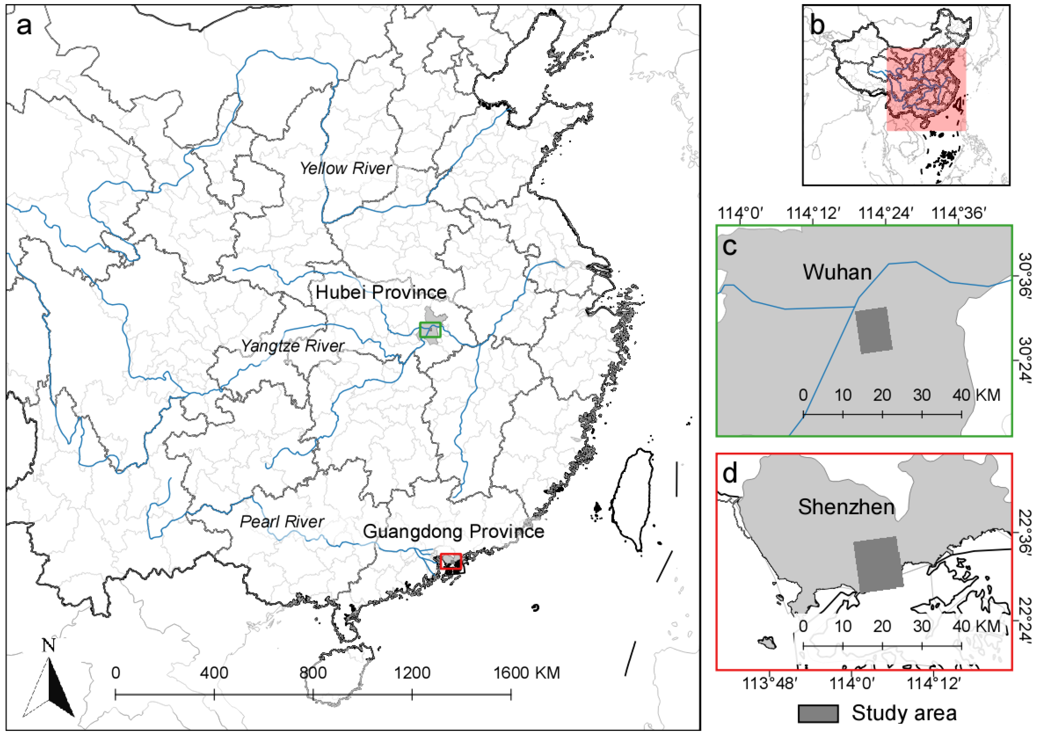
Figure 2.
City and urban village (UV) landscapes in different views: (a,b) are city and UV landscape diagrams; and (c,d) are the corresponding remote sensing images; (e,f) show aerial views of a typical urban area and a UV in Shenzhen.
Figure 2.
City and urban village (UV) landscapes in different views: (a,b) are city and UV landscape diagrams; and (c,d) are the corresponding remote sensing images; (e,f) show aerial views of a typical urban area and a UV in Shenzhen.
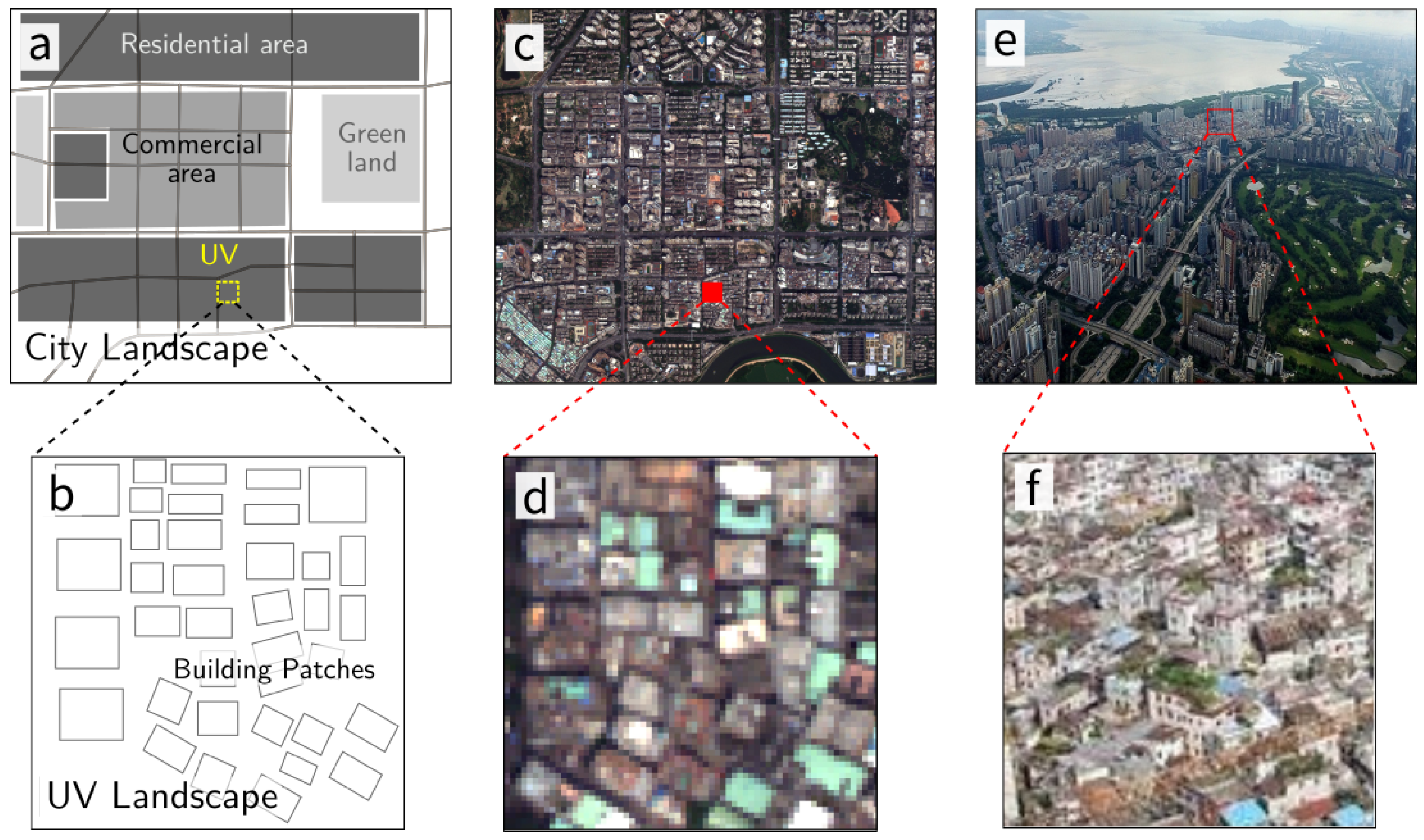
Figure 3.
The moving window strategy for dividing the city landscape. Scenes are half-overlapped.

Figure 4.
Raw classification results of UVs and the final results with manual processing for Shenzhen (a–c) and Wuhan (d–f).
Figure 4.
Raw classification results of UVs and the final results with manual processing for Shenzhen (a–c) and Wuhan (d–f).

Figure 5.
Average Kappa values produced in the classification of the Shenzhen images with four different settings, where TDS and SW respectively mean whether target domain samples and sample weighting were used in the classification.
Figure 5.
Average Kappa values produced in the classification of the Shenzhen images with four different settings, where TDS and SW respectively mean whether target domain samples and sample weighting were used in the classification.
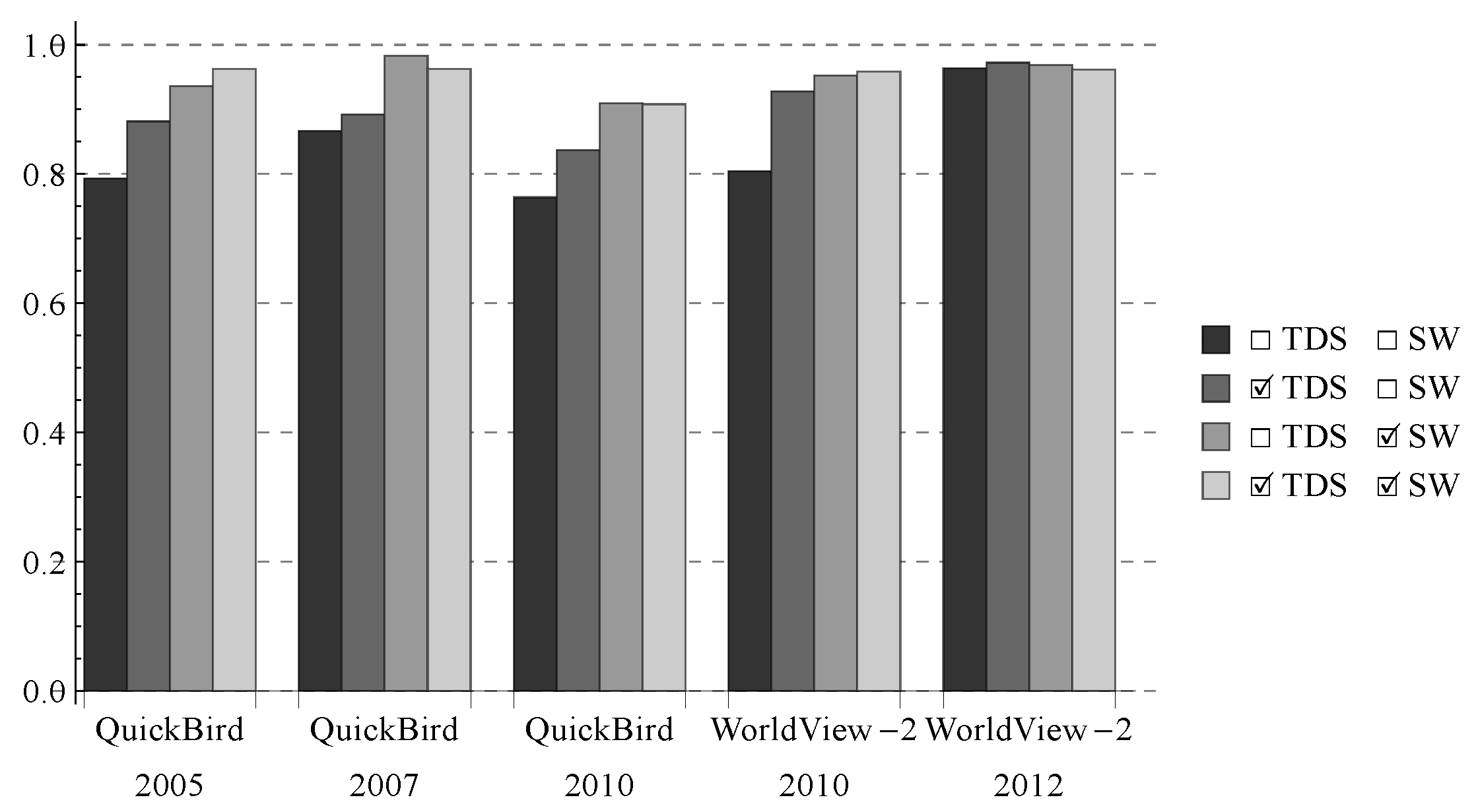
Figure 6.
Average Kappa values produced for the Shenzhen images with different scene sizes.

Figure 7.
The left image, extracted from the Shenzhen 2012 WorldView-2 image, shows a UV; the other images are the corresponding classification results produced with different scene sizes.
Figure 7.
The left image, extracted from the Shenzhen 2012 WorldView-2 image, shows a UV; the other images are the corresponding classification results produced with different scene sizes.

Figure 8.
Average rank of the metric significance computed by the vector angle (VA) and mean decrease in the Gini index (MDG), respectively.
Figure 8.
Average rank of the metric significance computed by the vector angle (VA) and mean decrease in the Gini index (MDG), respectively.

Figure 9.
Evolution of UVs at the city scale illustrated by landscape metrics.
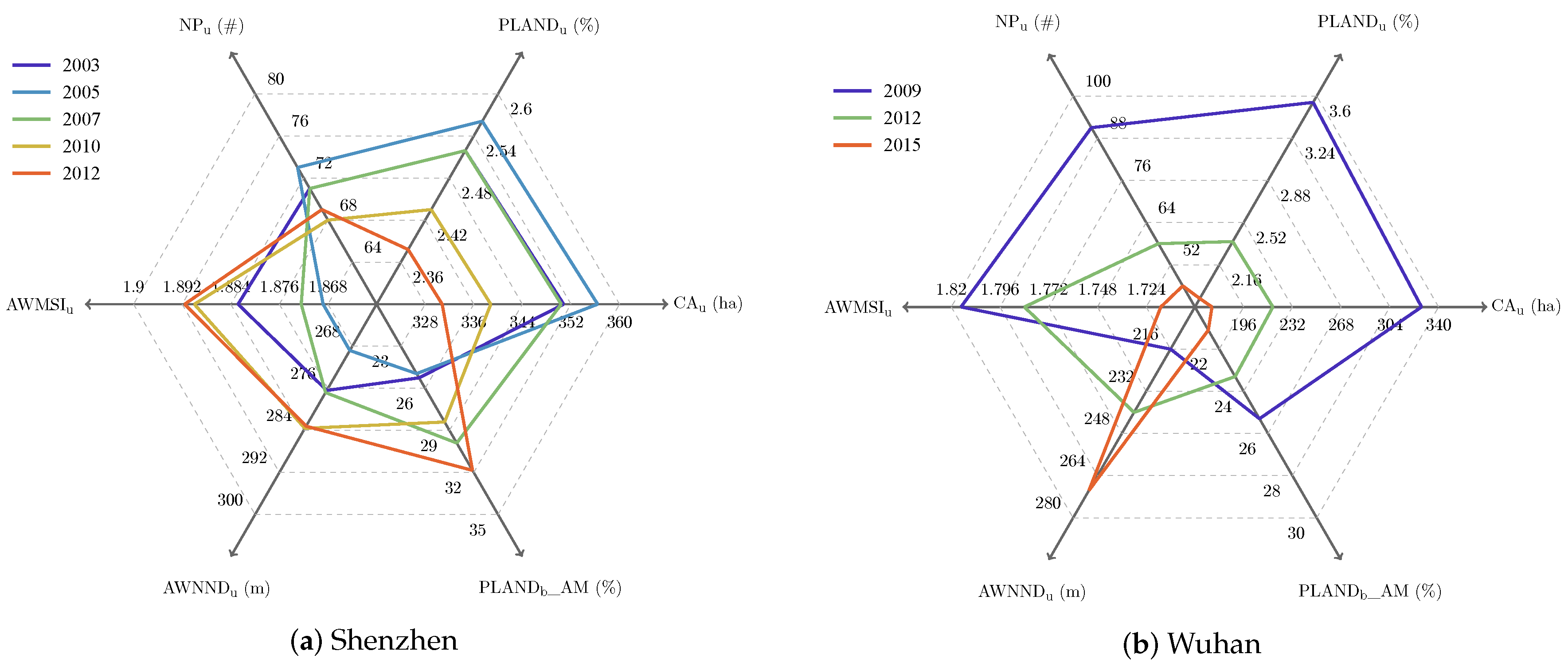
Figure 10.
Metric statistics for the Shenzhen and Wuhan study areas, where the first five bars and the last three bars in each plot respectively belong to Shenzhen and Wuhan.
Figure 10.
Metric statistics for the Shenzhen and Wuhan study areas, where the first five bars and the last three bars in each plot respectively belong to Shenzhen and Wuhan.
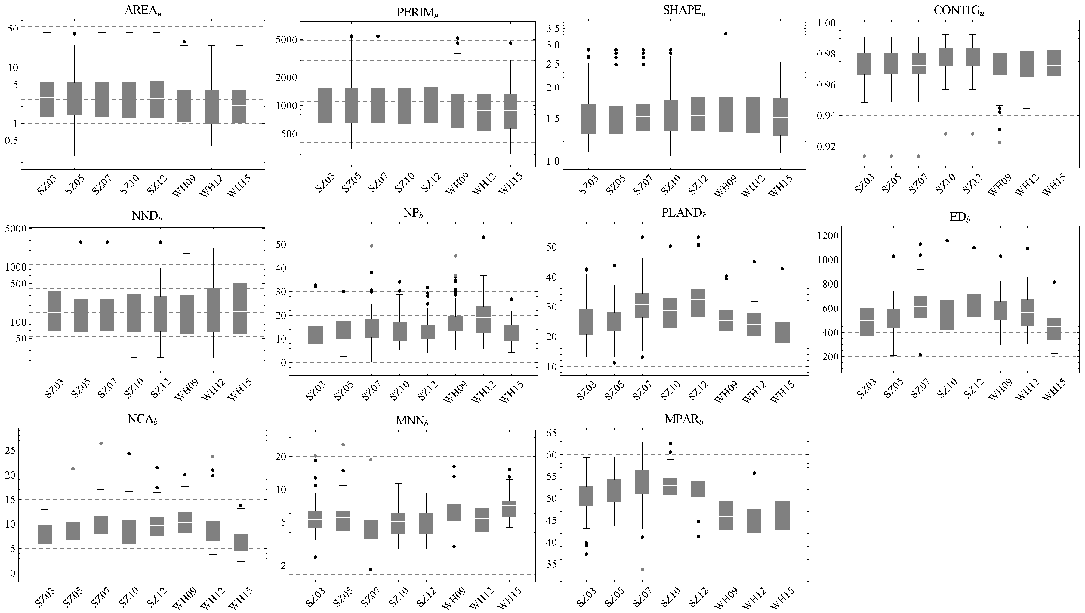
Figure 11.
Spatial clustering of UVs produced by different metrics in Shenzhen. From left to right, the year of each image is 2003, 2005, 2007, 2010 and 2012. Red and blue colors respectively indicate metric values above and below the average. In the legend, “High-High” and “Low-Low” represent positive spatial correlation, and “High-Low” and “Low-High” represent negative spatial correlation.
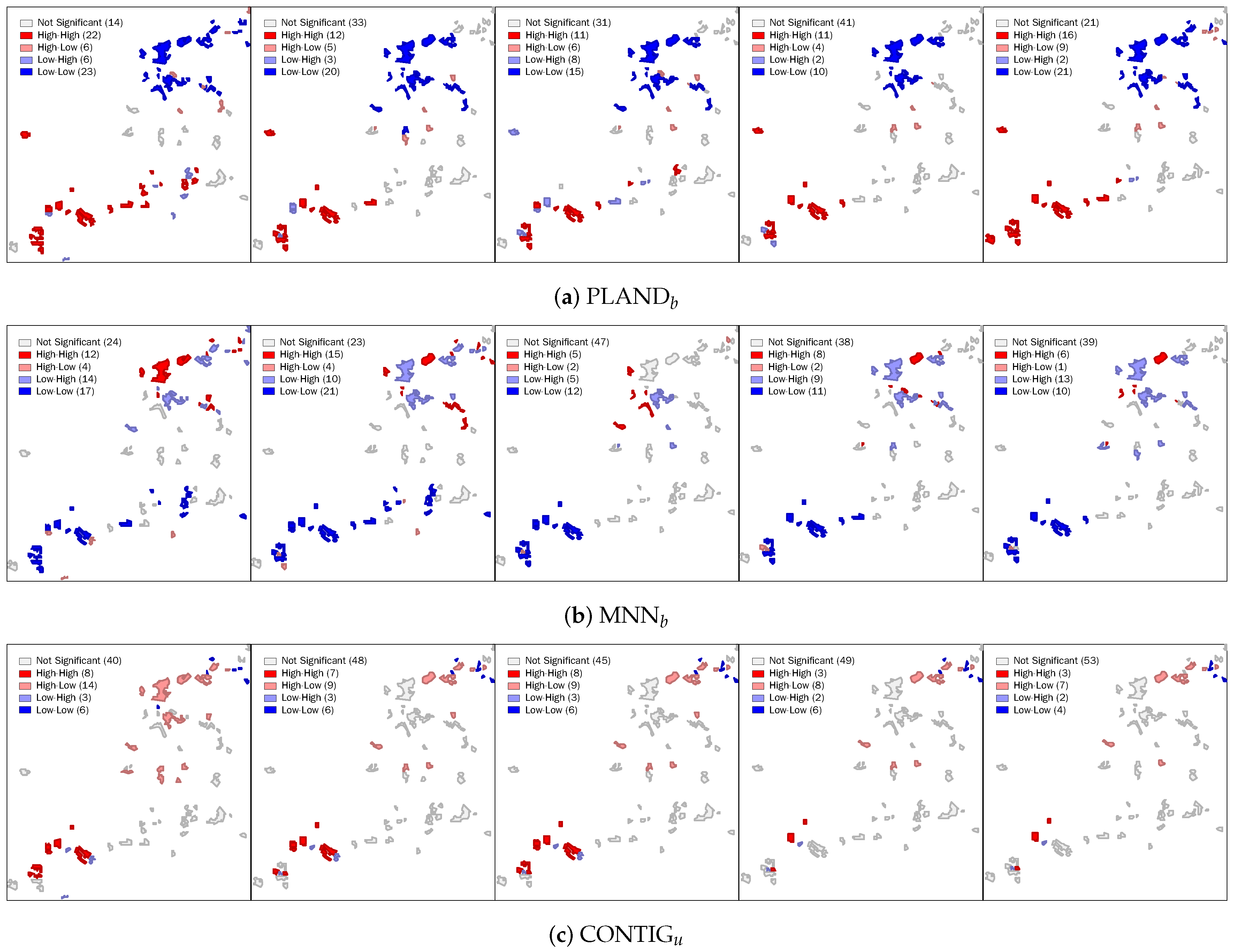
Figure 12.
UVs in the urban environment.

Table 1.
Overview of the Shenzhen and Wuhan multi-temporal data.
| Study Area | Satellite | Date | Resolution | Image Size (Pixel) |
|---|---|---|---|---|
| Shenzhen | QuickBird | January 2003 | 2.4 m | 5360 × 4507 |
| December 2005 | ||||
| December 2007 | ||||
| May 2010 | ||||
| WorldView-2 | November 2010 | 2 m | 6433 × 5409 | |
| March 2012 | ||||
| Wuhan | GeoEye-1 | January 2009 | 2 m | 5550 × 4156 |
| December 2012 | ||||
| WorldView-2 | November 2015 |
Table 2.
List of landscape metrics for the city-UV structure.
| Level | Abbrev. | Metric | Formula |
|---|---|---|---|
| AREA | Area of the UV (ha) | ||
| PERIM | Perimeter of the UV (m) | ||
| Patch | SHAPE | Shape Index of the UV | |
| CONTIG | Contiguity Index of the UV | ||
| NND | Distance to the nearest neighboring UV (m) | ||
| CA | Total area of UVs (ha) | ||
| PLAND | Percentage of UV areas in the city (%) | ||
| Landscape | NP | Number of UVs (#) | n |
| AWMSI | Area-weighted mean shape index | ||
| AWNND | Area-weighted nearest-neighbor distance |
Where n is the number of UVs, A is the total landscape area, is the area of UV, is the perimeter of UV, R is the number of pixels in UV, c is a specific convolution kernel [49], is the corresponding region of UV, centered at pixel r, and is the distance from UV to the nearest UV.
Table 3.
List of landscape metrics for the UV-building structure, which are all landscape-level metrics.
Table 3.
List of landscape metrics for the UV-building structure, which are all landscape-level metrics.
| Abbrev. | Metric | Formula |
|---|---|---|
| NP | Number of patches (#) | n |
| PLAND | Percentage of landscape (%) | |
| LPI | Largest patch index (%) | |
| MPS | Mean patch size (ha) | |
| PSSD | Patch size standard deviation (ha) | |
| ED | Edge density (m/ha) | |
| CLAND | Core area percent of landscape (%) | |
| NCA | Number of core areas (#) | |
| MCA | Mean core area per patch (ha) | |
| CASD | Patch core area standard deviation (ha) | |
| TCAI | Total core area index (%) | |
| MCAI | Mean core area index (%) | |
| MNN | Mean nearest-neighbor distance (m) | |
| NNSD | Nearest-neighbor standard deviation (m) | |
| MPI | Mean proximity index | |
| PISD | Proximity index standard deviation | |
| MSI | Mean shape index | |
| AWMSI | Area-weighted mean shape index | |
| MPFD | Mean patch fractal dimension | |
| AWMPFD | Area-weighted mean patch fractal dimension | |
| MPER | Mean patch extent ratio | |
| ERSD | Patch extent ratio standard deviation | |
| MPAR | Mean patch aspect ratio | |
| ARSD | Patch aspect ratio standard deviation | |
| PVAI | Patch vegetation area index |
Where n is the number of buildings, is the total area of buildings, A is the total landscape area, is the area of building , is the perimeter of building , is the number of disjunct core areas in building based on specified buffer width (3 pixels in this paper), is the core area of building , is the distance from building to the nearest building, is the area of building within a specified neighborhood (10 pixels in this paper) of building , is the distance between building (located within a specified neighborhood) and building , is the area ratio of building and its minimum enclosing rectangle, is the length-width ratio of the minimum enclosing rectangle of building and is the area of vegetation within a specified neighborhood (3,5,7,9 pixels in this paper) of building . In addition, PLAND, MPS and PSSD were also computed for the UV-vegetation landscape in the classification.
Table 4.
Average accuracies (Kappa value, omission error and commission error from top to bottom) produced with different training samples in the classification of the Shenzhen images.
Table 4.
Average accuracies (Kappa value, omission error and commission error from top to bottom) produced with different training samples in the classification of the Shenzhen images.
| Training Samples | QuickBird | QuickBird | QuickBird | WorldView-2 | WorldView-2 |
|---|---|---|---|---|---|
| Used in Classification | 2005 | 2007 | 2010 | 2010 | 2012 |
| 0.864 | 0.920 | 0.853 | 0.919 | 0.945 | |
| Target domain samples | 0.158 | 0.102 | 0.105 | 0.023 | 0.020 |
| 0.013 | 0.005 | 0.040 | 0.042 | 0.014 | |
| Source domain | 0.793 | 0.866 | 0.764 | 0.804 | 0.964 |
| samples without | 0.124 | 0.152 | 0.308 | 0.259 | 0.017 |
| sample weighting | 0.069 | 0.018 | 0.006 | 0.004 | 0.012 |
| Source domain | 0.936 | 0.983 | 0.909 | 0.953 | 0.968 |
| samples with | 0.010 | 0.005 | 0.038 | 0.006 | 0.001 |
| sample weighting | 0.028 | 0.007 | 0.029 | 0.025 | 0.019 |
| (The proposed) |
Table 5.
Highest Kappa values produced for the Wuhan images.
| Sample Sources | The Collection of Metrics | GeoEye-1 | GeoEye-1 | WorldView-2 |
|---|---|---|---|---|
| 2009 | 2012 | 2015 | ||
| Wuhan | Table 3 | 0.737 1 | 0.730 | 0.714 |
| Shenzhen + Wuhan | Table 3 | 0.777 | 0.835 | 0.764 |
| Shenzhen + Wuhan | Propagated | 0.803 | 0.790 | 0.779 |
| Shenzhen + Wuhan | Reduced by VA | 0.794 | 0.812 | 0.665 |
| Shenzhen + Wuhan | Reduced by MDG | 0.794 | 0.779 | 0.765 |
1 This result was produced with labeled samples from the target domain, i.e., the 2009 GeoEye-1 image, because no earlier Wuhan samples were available.
Table 6.
Global Moran’s I of the landscape metrics showing significant spatial auto-correlation.
| City | Year | NP | PLAND | ED | NCA | MNN |
|---|---|---|---|---|---|---|
| 2003 | 0.17 ‡ | 0.4 ‡ | 0.38 ‡ | 0.29 ‡ | 0.12 ‡ | |
| 2005 | 0.03 | 0.16 ‡ | 0.18 ‡ | 0.19 ‡ | 0.08 ‡ | |
| Shenzhen | 2007 | 0 | 0.08 ‡ | 0.07 † | 0.05 † | 0.04 † |
| 2010 | 0.05 † | 0.16 ‡ | 0.17 ‡ | 0.2 ‡ | 0.06 † | |
| 2012 | 0 | 0.2 ‡ | 0.19 ‡ | 0.19 ‡ | 0.05 † | |
| 2009 | 0.07 ‡ | −0.05 | −0.04 | 0.01 | −0.02 | |
| Wuhan | 2012 | 0.14 ‡ | 0.08 † | 0.13 ‡ | 0.15 ‡ | 0.09 † |
| 2015 | 0.06 | 0.06 | 0.02 | 0.06 | −0.01 |
This value is significant at the level of 0.05. This value is significant at the level of 0.01.
© 2017 by the authors. Licensee MDPI, Basel, Switzerland. This article is an open access article distributed under the terms and conditions of the Creative Commons Attribution (CC BY) license (http://creativecommons.org/licenses/by/4.0/).
Share and Cite
MDPI and ACS Style
Liu, H.; Huang, X.; Wen, D.; Li, J. The Use of Landscape Metrics and Transfer Learning to Explore Urban Villages in China. Remote Sens. 2017, 9, 365. https://doi.org/10.3390/rs9040365
AMA Style
Liu H, Huang X, Wen D, Li J. The Use of Landscape Metrics and Transfer Learning to Explore Urban Villages in China. Remote Sensing. 2017; 9(4):365. https://doi.org/10.3390/rs9040365
Chicago/Turabian StyleLiu, Hui, Xin Huang, Dawei Wen, and Jiayi Li. 2017. "The Use of Landscape Metrics and Transfer Learning to Explore Urban Villages in China" Remote Sensing 9, no. 4: 365. https://doi.org/10.3390/rs9040365
Note that from the first issue of 2016, this journal uses article numbers instead of page numbers. See further details here.