
An Improved RANSAC for 3D Point Cloud Plane Segmentation Based on Normal Distribution Transformation Cells


1
School of Resource and Environment Sciences, Wuhan University, 129 Luoyu Road, Wuhan 430079, China
2
Collaborative Innovation Centre of Geospatial Technology, Wuhan University, 129 Luoyu Road, Wuhan 430079, China
*
Author to whom correspondence should be addressed.
Remote Sens. 2017, 9(5), 433; https://doi.org/10.3390/rs9050433
Submission received: 13 March 2017
/
Revised: 9 April 2017
/
Accepted: 30 April 2017
/
Published: 3 May 2017
(This article belongs to the Special Issue Fusion of LiDAR Point Clouds and Optical Images)
Abstract
:Plane segmentation is a basic task in the automatic reconstruction of indoor and urban environments from unorganized point clouds acquired by laser scanners. As one of the most common plane-segmentation methods, standard Random Sample Consensus (RANSAC) is often used to continually detect planes one after another. However, it suffers from the spurious-plane problem when noise and outliers exist due to the uncertainty of randomly sampling the minimum subset with 3 points. An improved RANSAC method based on Normal Distribution Transformation (NDT) cells is proposed in this study to avoid spurious planes for 3D point-cloud plane segmentation. A planar NDT cell is selected as a minimal sample in each iteration to ensure the correctness of sampling on the same plane surface. The 3D NDT represents the point cloud with a set of NDT cells and models the observed points with a normal distribution within each cell. The geometric appearances of NDT cells are used to classify the NDT cells into planar and non-planar cells. The proposed method is verified on three indoor scenes. The experimental results show that the correctness exceeds 88.5% and the completeness exceeds 85.0%, which indicates that the proposed method identifies more reliable and accurate planes than standard RANSAC. It also executes faster. These results validate the suitability of the method.
1. Introduction
As laser scanning technologies have developed, they have been widely used in applications such as 3D city modeling [1,2], road inventory study [3,4,5], Simultaneous Localization and Mapping (SLAM) [6,7] and indoor mapping [8,9,10]. Being efficient and of high density, the point clouds captured by airborne laser scanning (ALS), terrestrial laser scanning (TLS), and mobile laser scanning (MLS) can be employed in fast monitoring of urban environments. The huge point-cloud data available from indoor environments have inspired deep understanding of the data on the semantic level to meet the demands of indoor mapping and reconstruction. Objects with planar surfaces such as ceilings, walls and floors abound in indoor environments, and can semantically provide a compressive representation of the point clouds; typically, the data-compression rate can reach over 90% [11,12]. The point clouds of these types of objects have a planar geometric appearance, and the plane can be extracted. Plane segmentation has been explored for years and is still a very hot and complex task in indoor mapping and reconstruction. Both organized and unorganized point clouds have been the focus of much research. Organized point clouds resemble organized image-like structures, where the data are split into rows and columns; therefore, it is easy to use the neighbor information in the organized structure. In contrast, unorganized point clouds vary in size, density and point ordering, and the neighbor information cannot be used directly. Therefore, plane segmentation for unorganized point clouds is more complex. However, unorganized point clouds require less storage space and are more suitable for high-density point-cloud storage. In this study, the input consists of unorganized point clouds acquired by MLS in indoor environments, which require an efficient method for processing.
Point cloud segmentation plays an important role in point cloud processing [12,13]. As one of the most important part of point cloud segmentation, plane-segmentation methods can be generally classified into three categories [14,15]: region-based methods, Hough transform and Random Sample Consensus (RANSAC). Region-based methods assume that neighboring points within the same region have similar properties. Neighborhood information is used to combine nearby points that have similar properties to obtain isolated regions [13,16]. Region-based methods are simple, but they have problems with over or under segmentation, are very sensitive to noise and are time consuming [13]. When the transitions between regions are smooth, finding a termination criterion for region-based methods becomes difficult [17]. The Hough transform is a method for detecting parameterized objects and is typically used to find lines and circles in 2D situations. For 3D point-cloud plane segmentation, every point in the Hough space corresponds to a plane in the object space. First, the Hough space is discretized and represented by an accumulator. Then, plane segmentation becomes a peak-detection problem in the accumulator [15]. The Hough transform is robust for shape extraction even on noisy datasets. However, it demands large amounts of memory and computational time [13]. The study by Tarsh-Kurdi et al. [18] suggested that RANSAC would be more efficient than Hough transform. While the RANSAC algorithm is effective in the presence of noise and outliers, it has the obvious drawback that the planes detected by RANSAC may not belong to the same planar surface; spurious planes may appear [19,20]. This often occurs in complex indoor environments when using the RANSAC method to successively extract planes. RANSAC iteratively and randomly samples 3 points as a minimum subset to generate the hypothesis plane and then tests all the remaining points in the point cloud to detect the best plane, which is defined as the plane with the highest percentage of inliers; however, there is uncertainty in the process of hypothesis generation. Even for the plane with the largest percentage of inliers, the three randomly selected points may not belong to the same plane. Some robust methods [20,21] have been adopted to address the spurious-plane problem; however, these are all point-based, which is not efficient in an indoor environment.
The main contribution of this paper is that the planar NDT cell is selected as a minimal sample on the surface of the same plane to ensure the correctness of sampling. A primary plane is detected first and the remaining points are tested against it to obtain a complete plane. The proposed method can improve the correctness of plane segmentation and eliminate the spurious-plane problems of standard RANSAC. An iterative reweighted least-squares (IRLS) approach is also used for plane fitting to improve the reliability and accuracy of a detected plane.
2. Related Works
2.1. NDT Methods
Because point-cloud data abound with geometric information, it is necessary to take neighbor points into consideration during point-cloud processing. Point features are commonly used and are calculated by the neighbors of each point. For example, the normal, curvature and roughness features are used for point-cloud segmentation and compression. Methods based on voxel grids and octrees [22,23] are often used to improve the efficiency of plane segmentation. The proposed method is based on Normal Distribution Transform (NDT) cells, which is a discrete representation of point-cloud space that takes each cell into consideration rather than each point. NDT is a concept similar to super-voxels and sub-windows.
Super-voxels was proposed by Ahmad et al. [24] and is used for point-cloud segmentation. First, the 3D point cloud is segmented into voxels. Then, the voxels are characterized by several attributes, transforming them into super-voxels. Finally, these are joined together using a link-chain method to create objects.
Xiao et al. [12] proposed two complementary strategies, a named sub-window-based region-growing algorithm for structured environments and a hybrid region-growing algorithm for unstructured environments. A sub-window is a moving window suitable for organized point-cloud representation. They classified the sub-windows into two categories based on their shapes: planar and non-planar. The algorithms are faster than the point-based region-growing algorithms when a proper window size is set.
NDT was first proposed by Biber and Strasser [25] for 2D point-cloud registration in 2013 and was later extended to three dimensions [26]; however, to the best of our knowledge, very few works [27] use NDT for point-cloud segmentation. The concept underlying NDT is to subdivide the space occupied by the scan into a grid of cells (squares in 2D and cubes in 3D). A Probability Density Function (PDF) is computed for each cell, based on the point distribution within the cell. The NDT feature is different from the point-based feature because NDT considers points within a cell, while the point-based feature takes the neighbors of a point into account. Additionally, unlike the sub-window approach, NDT is suitable for both organized and unorganized point-cloud descriptions. There are two NDT discretization strategies. One is to split the point cloud into a grid of regular size [28]. Another is to construct a 3D-NDT that uses an irregular grid discretization, such as Octree discretization, which was explored earlier by Magnusson [29].
2.2. RANSAC
RANSAC was introduced by Fischer and Bolles [30] in 1981 and is widely used for shape detection [13,20,31]. The RANSAC algorithm mainly involves performing two iteratively repeated steps on a given point cloud: generating a hypothesis and verification. First, hypothesis shapes are generated by randomly selecting a minimal subset of n points and estimating the corresponding shape-model parameters. A minimal subset contains the smallest number of points required to uniquely estimate a model; for example, 3 points are needed to determine a plane. Then, the remaining points in the point cloud are tested with the resulting candidate shapes to determine how many of the points are well approximated by the model. After a certain number of iterations, the shape that possesses the largest percentage of inliers is extracted and the algorithm continues to process the remaining data. The plane is often fitted by the least-squares (LS) method, but this approach is often not robust to outliers when detecting planes repeatedly.
RANSAC assumes that a model generated from a contaminated minimal sample will have low support, thus making it possible to distinguish between correct and incorrect models [32,33,34]. Spurious surfaces may appear when planes are repeatedly detected in succession (Figure 1). Various methods have been adopted to address the spurious-plane problem and improve the robustness of RANSAC; for example, MSAC and MLESAC [21] use loss functions rather than fixed thresholds to evaluate the contribution of the inliers based on the point-to-plane distance. A soft-threshold voting function [20] based on two weight functions is used to improve the segmentation quality, which considers both the point-plane distance and the consistency between the normal vectors. However, it requires estimation of the normal at each point, which is not efficient in high-density point clouds.
According to [32], the time complexity in RANSAC depends on the subset size, the inlier ratio and the number of data points. RANSAC's runtimes can be prohibitively high in some cases. Schnabel et al. [31] presented a more efficient RANSAC for point-cloud shape detection—including plane shapes. Octree was used to establish spatial proximity among samples and its scoring function tests only a local subset of samples. Local sampling, by selecting points inside each node, is used to avoid meaningless hypotheses. However, spatial proximity does not guarantee coplanarity; thus, the technique does not work well for the spurious-plane problem.
3. Proposed Methods
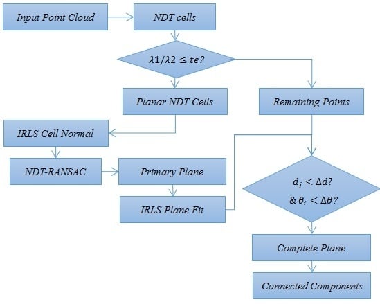
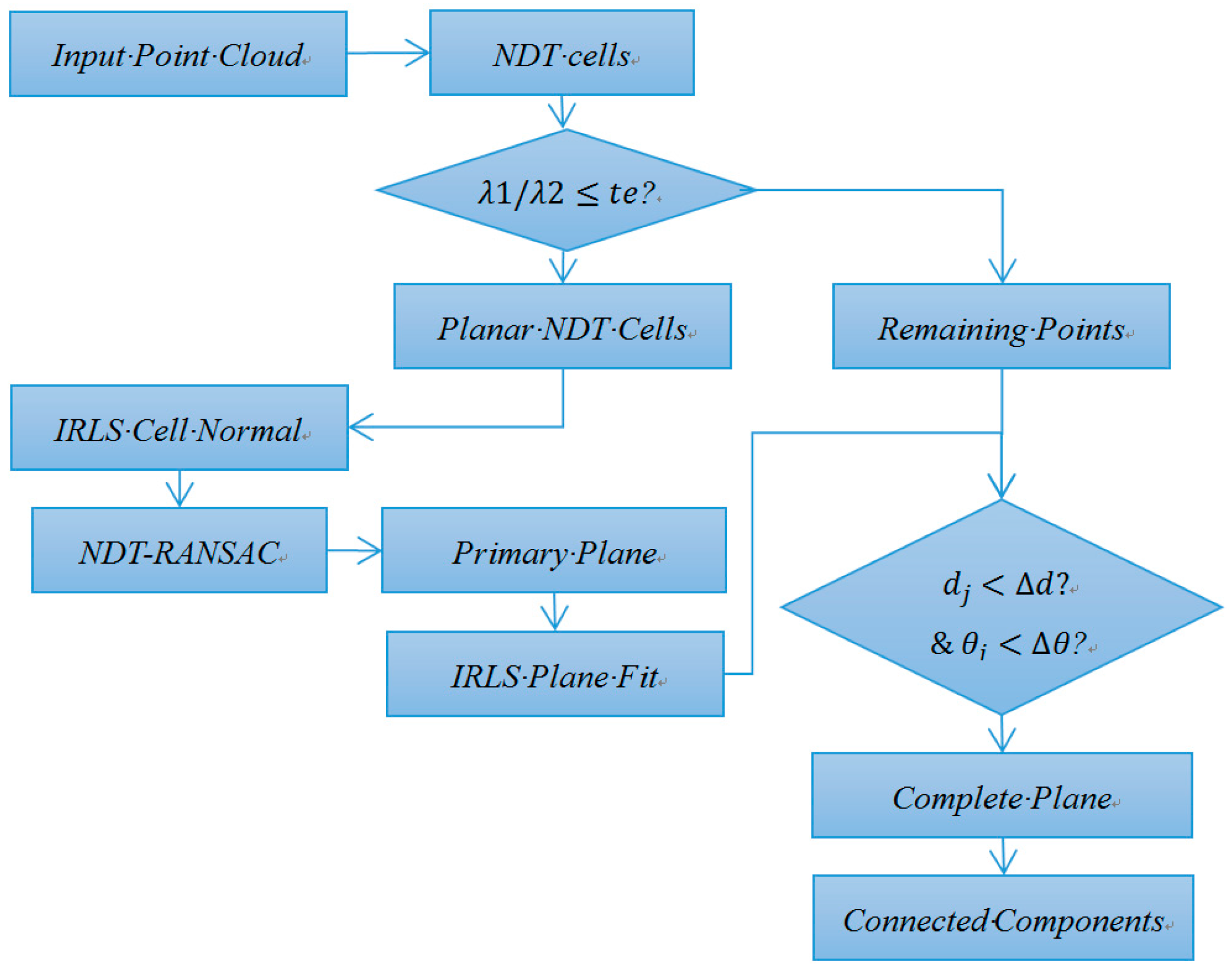
The proposed plane-segmentation method is described in detail in this section. The first step is to calculate the NDT features by subdividing the point-cloud space into a grid of NDT cells and then classifying the NDT cells into planar and non-planar cells. Then, an NDT-based RANSAC algorithm is applied to obtain reliable primary planes. The aim of the probability analysis is to determine when the iteration should stop. Afterward, an iterative reweighted least-square approach is used for normal calculation and plane fitting. Finally, the remaining non-planar points are tested with the primary planes to obtain complete planes. Alternatively, connected-component analysis can be utilized to divide unconnected components into parts. The main steps involved in the NDT-RANSAC method are depicted in Figure 2.
3.1. NDT Feature
The 3D NDT discretizes the point cloud using a set of cells and models the observed points within each cell with a normal distribution. Each cell in the 3D grid is associated with a sampled mean and a covariance representing the multivariate normal distribution [27]. Each cell contains at least points. The covariance matrix is a positive-definite matrix that can be used to describe the shape of each cell. The eigenvalues and the corresponding eigenvectors of the covariance matrix are computed for each cell.
- If , the distribution of the NDT cell is linear.
- If it is nonlinear and , the distribution of the NDT cell is planar.
- If no eigenvalue is times larger than another one, the distribution of the NDT cell is spherical.
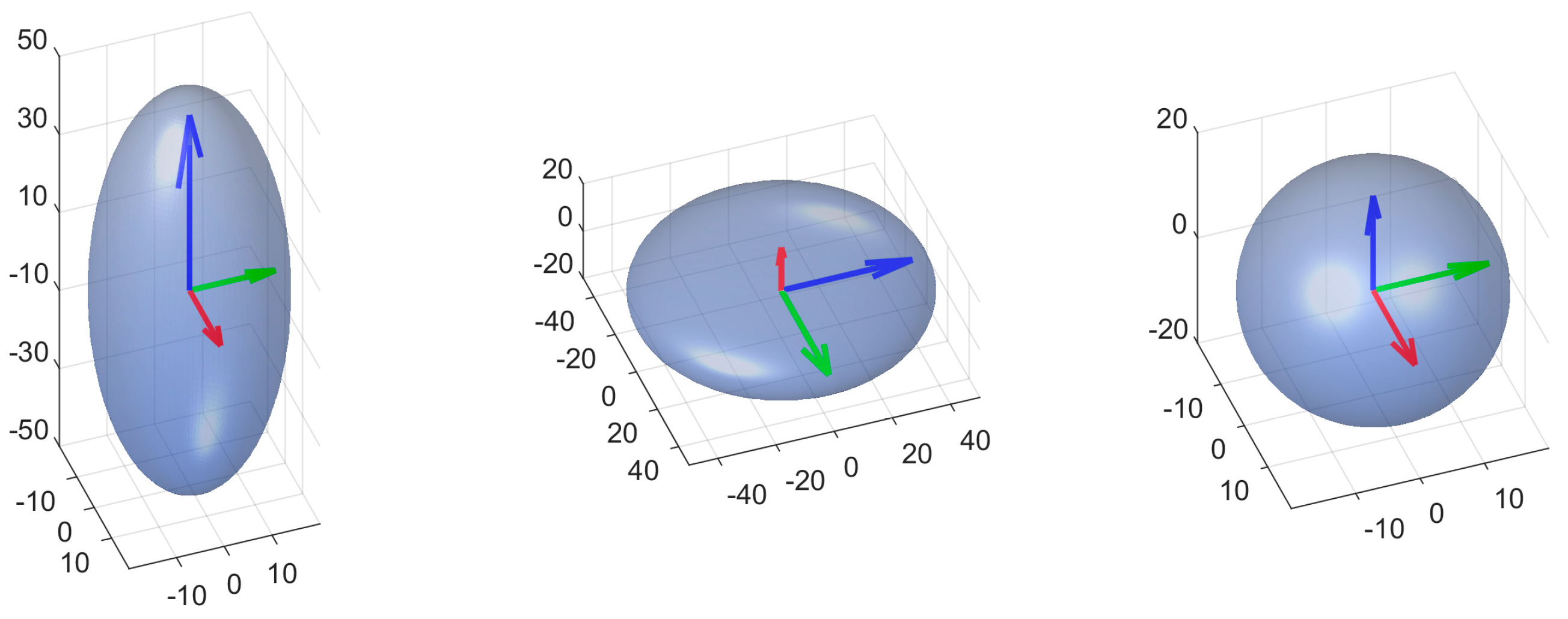
When te ∈ [0, 1] is set to an appropriate, the NDT cells can be classified as linear, planar or spherical. The covariance ellipsoid [35,36] is used to describe the appearance of NDT cells (Figure 3), where each axis of the ellipsoid represents a principal component and the square root of the eigenvalues corresponds to three semi-axes’ length of ellipsoid. The eigenvalues λ1, λ2, λ3 correspond to the third axis, the second axis and the first axis of the ellipsoid, respectively. In other words, the magnitudes of the ellipsoid axes depend on the variance of the data. Focusing on planar surfaces in this paper, te is given a small value to classify NDT cells as planar or non-planar. The te value constrains the ratio between third axis and second axis, for example, if te = 1/25 = 0.04, the ratio between third axes and second axes is 1/5; if te = 1/100 = 0.01, the ratio between third axis and second axis is 1/10. We recommend te < 0.04 empirically. The smaller the te value is, the more flat the NDT cell is.
Due to the existence of measure errors, the setting of parameter should consider the noisy level of plane surfaces in point cloud and the NDT cell size in practice. The following empirical equation can be adopted to choose a proper te and cell size s.
where is the noise level of a measured plane (the average point distance to the plane, which depends on the accuracy of laser range scanner and can be roughly estimated from the point cloud). An indoor scene from Possum’s Dataset [36] is shown in Figure 4a, the point cloud is discretized into NDT cells (Figure 4b). The surface edges are classified as non-planar cells. The working details of the NDT Feature Calculation are described in Algorithm 1.
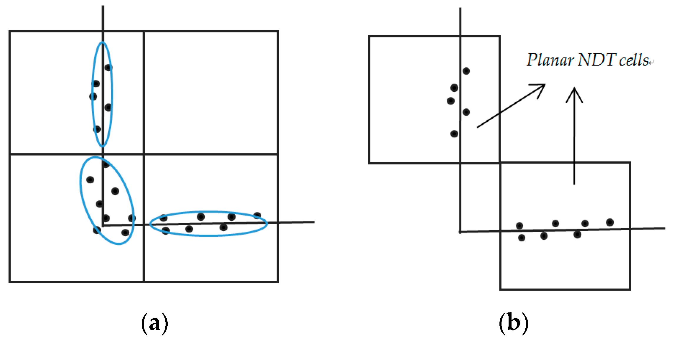
By calculating the NDT feature of each cell, the planar NDT cells can be marked. Cells on the surface edges are classified as non-planar cells (Figure 5). When a minimal subset for a plane is randomly selected, a point on the surface of this plane is more likely to be selected, resulting in the omission of less important planes and, thus, reducing the probability of extracting spurious planes.
| Algorithm 1. NDT Feature Calculation. |
| Input: P: an unorganized point cloud; : cell size; : a threshold to classify cells as planar or non-planar Initialize: ; // NDT cell list ; // planar NDT cell list ; // remaining points for each point in P Subdivide the space occupied by the scan into a grid of cubes ; Calculate the encoding of each point , which indicates the index of the cell; end for for each cell in Calculate the mean of the points in each cell; Calculate the covariance of each NDT cell; Eigen-decomposition for , get the eigenvalues and the corresponding eigenvectors of ; if Add cell into ; else if Add points into ; end if end for return |
3.2. NDT-RANSAC Plane Segmentation
NDT cells are suitable for plane segmentation based on the following two assumptions. First, most NDT cells located on planar surfaces have a planar appearance. Second, NDT cells from the same surface have similar plane parameters. These assumptions are similar to those in [12,31].
NDT-RANSAC randomly samples a minimal subset of one cell from the planar NDT cells. The normal of the cell is used as the plane parameter. Then, two thresholds are applied, which consider both the gravity distance from the point to the plane and the angular differences of the cells’ normals to the plane. If the distance and angular differences are smaller than given thresholds, the cells can be treated as being on the candidate plane. When the data consists of inliers and outliers, traditional RANSAC assumes that the distribution of inlier data can be explained by some set of model parameters, while outliers are data that do not fit the model. However, if the randomly selected minimal set contains outliers, spurious planes appear. When the points in an NDT cell have a planar appearance, they are likely from the same plane; thus, the cell selected as a minimal subset is suitable and intuitive, which makes the detected plane reliable. The working details of NDT-RANSAC are described in Algorithm 2. The NDT-cell-based method consumes less time than the point-based method because it does not need to estimate the normal of every point. Instead, the time consumption depends on the cell size and point density. The larger the NDT cells and the higher the density in each cell, the smaller the time cost.
| Algorithm 2. NDT-RANSAC Plane Segmentation. |
| Input: : planar NDT cell list : non-planar points Initialize: : plane surface while randomly sample a cell c; then, its gravity and normal are used as plane parameter // Calculate the support set for each cell in ; ; if add to ; end if If then ; recompute from Equation (3) using ; end if ; end while refine plane ; for each point in ; ; if and add points in plane ; End if end for |
3.3. Probabilities
The maximum number of iterations depends on the a priori probability of sampling inliers over the data. Given a point cloud P, N planar cells are classified and a plane ψ contains n cells. A minimum subset needs one cell to determine a plane. Then, of the data are inliers, which means that the probability of randomly selecting each cell in plane ψ in a candidate experiment is . Therefore, the probability of not finding any inliers after k iterations is .
To ensure with confidence that an outlier-free cell is sampled in NDT-RANSAC, we must process at least k candidate samples, where
The calculation of k is almost the same with standard RANSAC [20,31,37], the difference is for standard RANSAC. The parameter lies usually between 0.90 and 0.99 [37]. The asymptotic complexity of NDT-RANSAC is when the cost of each step is C. To continually detect m planes, the iteration terminates when the size of the remaining planar cells’ is insufficient to ensure the sampling of the cell with confidence , i.e., when
3.4. IRLS Normal Calculation and Plane Fitting
It is well known that least-squares plane fitting is not robust to outliers. In this section, we introduce an iterative reweighted least-squares (IRLS) method using the M-estimator for plane fitting. Given a surface point cloud, the plane-fitting problem can be described as fitting a set of N data points to a plane model. Let be the distance of the ith point to the plane. The standard least-squares method tries to minimize but when outliers exist in the data, it becomes unstable [38]. Outliers have such a strong effect on the minimization that the estimated parameters are distorted. The M-estimator is often used to reduce the effect of outliers. It replaces the squared residuals by another function of the residuals, yielding
where is a symmetric, positive-definite function with a unique minimum at zero that is chosen to be less increasing than square. The plane-fitting problem then becomes the following IRLS problem:
where the superscript k indicates the iteration number. The weight should be recomputed after each iteration for use in the next iteration.
For plane fitting, the distance from a point to the plane is
where n is the normal of the plane and is the mean of the point cloud. The plane-fitting problem is a constrained least-squares problem. We use the Lagrange multiplier method:
To find the minimum, we take the derivative and set it to zero. Thus, we obtain
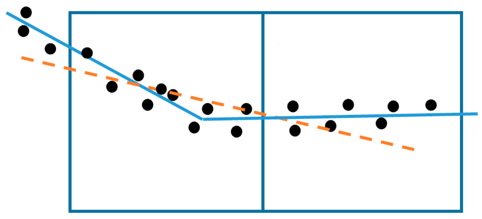
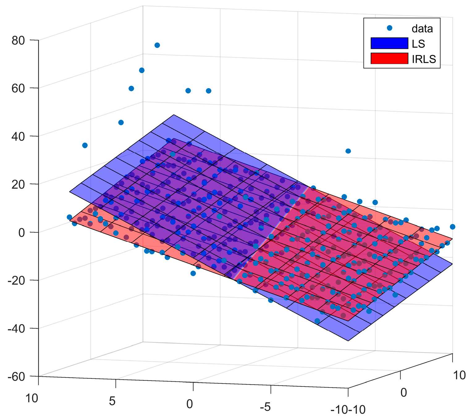
Therefore, the solution is to find the eigenvalues and eigenvectors of C. The details of the IRLS algorithm are given in Algorithm 3, and the convergence threshold is . The Welsch weighted function [39] is utilized in this study. Figure 6 shows an example of LS plane fitting result and IRLS plane-fitting result, the latter is more robust to outliers.
| Algorithm 3. IRLS Plane Fitting. |
| Input: : points on a detected plane : maximum number of iterations : threshold to terminate iterations Initialize: ; // last normal Calculate the mean of the plane point cloud ; Calculate the covariance of the plane point cloud; Eigen-decomposition of , get the eigenvalues and the corresponding eigenvectors of ; n = ; // take as the normal parameter of the plane; for k = 1 to ; ; Calculate Welsch function ; ; ; Eigen-decomposition of , the corresponding eigenvector of the smallest eigenvalue is used as plane parameter ; ; if then Terminate iterations; end if end for |
3.5. Connected-Component Analysis
The RANSAC method will extract a plane with many unconnected sub-regions. It is necessary to use connected-component analysis to divide such components into parts. A morphologic connected-component analysis is adopted with a threshold to find a sufficiently large plane and filter the points that are too far away.
3.6. NDT Cell Size
Xiao et al. [12] took structured and unstructured environments into consideration in their work. However, we make no such distinction; instead, we uniformly consider an unstructured environment. In practice, given a cell size for high-density TLS and MLS point clouds, the minimum number of points in a cell has no effect on the algorithm because it is easy to satisfy. However, for an uneven point cloud with a density that is not very high, the minimum number of points (for example, 10 points) will distinguish the sparse points. In this case, the minimum number of points should be properly set. The bounding box of the point cloud is calculated and the space is divided into cubes of fixed cell size based on the bounding box. Due to the nature of laser scanning, nearby points are dense while distant points are sparse. Inevitably, some cells will contain fewer than 10 points. When the point cloud is sparse in local space, a nearest-neighbor searching strategy is adopted in our method, which calculates the cell’s geometric features based on the neighboring points of the cell. This nearest-neighbor searching strategy extends the scope of the NDT cell. More points will be used to calculate the geometric features of the cell. We extend the size to at most two times larger than the cell itself.
4. Experimental Section
The method was tested on three datasets of indoor scenes. The Room-1 dataset corresponding to L9 room from the Rooms UZH Irchel dataset [40] was acquired using a Faro Focus 3D laser range scanner and has a high density of 91,352 points/m2. The scene itself is of a simple room with some furniture inside. The other two datasets captured by an MLS device were obtained from [41]. In these two datasets, the main sensor of the MLS device was a laser rangefinder (Hokuyo UTM-30 LX) mounted on a tilting unit. The local densities of the point clouds are uneven and are sparser than those of Room-1. These two scenes are complex; each contains a room, a corridor and some furniture. Clutter and occlusion are present in the datasets. In addition, a Faro Focus 3D laser range scanner is more accurate than a UTM-30 LX laser rangefinder. The basic parameters of the datasets are listed in Table 1. The algorithm was implemented in C++. All experiments were performed on a 2.30 Hz Intel Core i5-4670T processor with 8 GB of RAM.
To evaluate the quality of our proposed method for plane segmentation, we compared the calculated metrics of the individual planes with those of the ground-truth planes and calculated the metrics completeness, correctness and quality to evaluate the proposed method.
True Positive (TP): the number of planes detected both in the reference data and segmentation. False Positive (FP): the number of detected planes not found in the reference. False Negative (FN): the number of undetected ground-truth planes.
The reference backgrounds of the datasets were manually obtained based on the initial segmentation. The maximum-overlap metric [20,42] was used to find the correspondences between the reference and the plane-segmentation results. In this case, only one-to-one correspondences were considered in our experiments. The TP values in the reference and segmented data are always the same. To clearly illustrate the ability of our method to deal with spurious planes, we divided the FP into spurious planes (SFP) and non-spurious planes. The spurious planes do not correspond to any ground-truth plane, while non-spurious planes do correspond to ground-truth planes but are smaller than the given area threshold (i.e., 50% overlap). An evaluation metric called the spurious-plane rate (SR) was introduced to evaluate spurious planes in the segmentation results in this study:
For comparison, the standard RANSAC and NDT-RANSAC methods were applied to the three datasets. The parameters of the algorithm are specific to the density of the testing data but were always chosen to obtain the best results. The experiments are performed 30 times for each dataset. The parameters and thresholds adopted for Room-1 are as follows: . The segmentation result is shown in Figure 7, where the planar and non-planar NDT cells are colored in red and blue, respectively. For clarity, we removed the ceiling and floor of the room. It can be seen that the plane edges are classified as non-planar cells. Figure 7b shows the NDT-RANSAC plane-segmentation result using different colors.
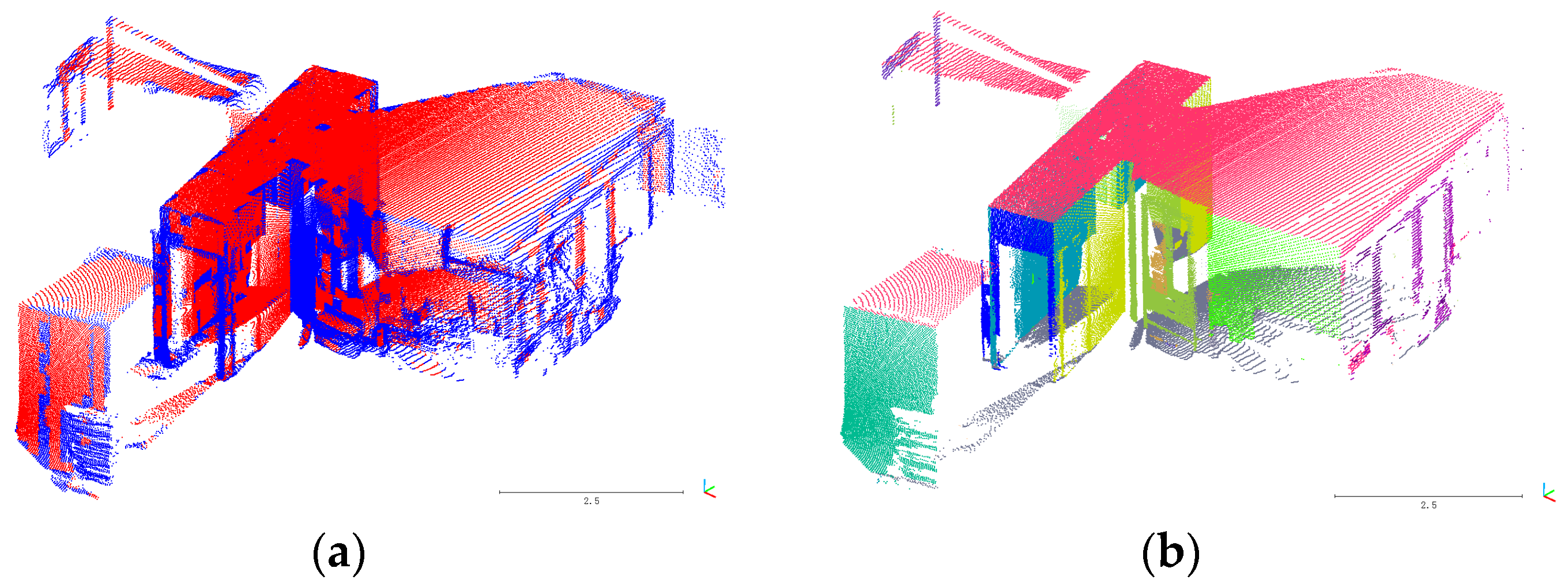
In order to accommodate the noise level of Room-2 dataset, the value is set to be greater than Room-1. The parameters and thresholds for the dataset were set as follows: In this experiment, only large-area planes are extracted and verified as background planes (for example, those with areas of at least ). A typical segmentation result for Room-2 is shown in Figure 8b). Different color represents different plane segment. Figure 9 shows a NDT cell-classification result and a plane-segmentation result for Room-3. The plane segments are shown in different colors. The parameters for this dataset were set to the same values as for Room-2.
5. Discussion
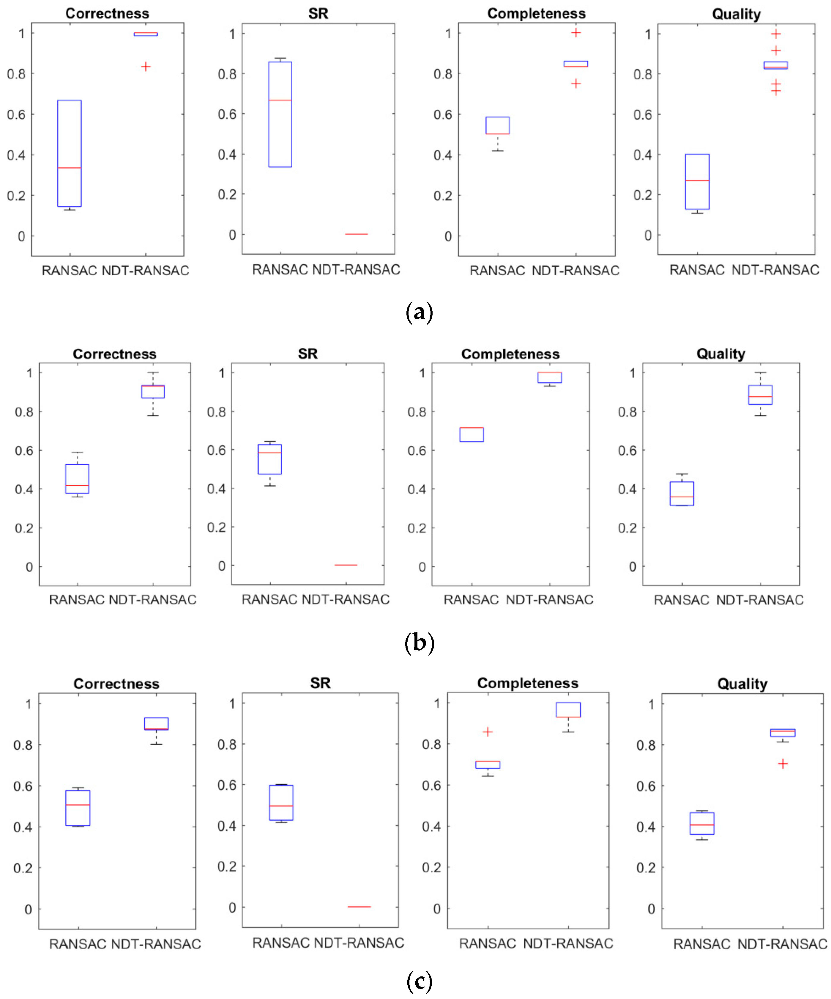
The experimental results were analyzed statistically, and the statistics on completeness, correctness, SR and quality of plane segmentation are shown in Figure 10a–c using boxplot. The average percentage values are summarized in Table 2.
As shown in Figure 10a, the NDT-RANSAC shows a better result than RANSAC in the experiment of Room-1. The average correctness increased from 37.3% to 98.3%, respectively, for this dataset and the completeness increased from 52.5% to 85.0%, respectively. It also showed a smaller fluctuation than standard RANSAC. The experimental results of Room-2 and Room-3 are shown in Figure 10b,c. Comparing the results from RANSAC and NDT-RANSAC, the average correctness increased from 45.9% to 90.4%, respectively. NDT-RANSAC achieved a high rate of completeness (98.1%)—higher than that of the standard RANSAC method (70.1%). In the experiment of Room-3, the proposed method achieved 88.5% correctness and 94.6% completeness, higher than the standard RANSAC method, which obtained 49.5% correctness and 71.4% completeness; thus, the proposed method improves the quality of plane segmentation. All the three experiments showed that the proposed method achieves higher average correctness and completeness than does standard RANSAC. However, comparing Figure 10a–c, the range of correctness and completeness values increased because the point clouds of Room-2 and Room-3 are noisier than that of Room-1.
The SR values of NDT-RANSAC for all three experiments are 0, which clearly shows that surplus planes have been eliminated in the experiments. However, the proposed method still finds some FP planes. The reason is that some detected planes are small (with overlap less than 50%) or have a low point density. The sparsity of the point cloud influences the segmentation results. If a larger value of is used, correctness will improve, but completeness may decrease. Moreover, the experiments indicate that for a larger cell size, the correctness will improve but the completeness may decrease. A smaller cell size requires more computer time and the plane surface will be divided into more pieces, making the plane discontinuous. This is because a small cell size increases the differences between the cells’ normals. When the size is too large, large-area planes will be identified but small planar surfaces will be ignored. This occurs because the minimum object size is larger than the cell size, which requires further consideration.
The average execution times are also shown in Table 2. It can be drawn that the proposed method reduced the time consumption for all three datasets. The processing time of Room-1 was 7.43 s, which reduced by over two orders of magnitude compared to the standard RANSAC. This result shows the advantage of our method in processing high-density point clouds. The processing time of Room-2 reduced from 5.57 s to 5.03 s. The processing time of Room-3 reduced from 5.29 s to 2.46 s. The improved time consumption occurs because the number of NDT cells is quite small compared to the number of points, which significantly reduces the computing time of the verification step during the iterations.
6. Conclusions
This paper presented a Normal Distribution Transformation Feature-based RANSAC (NDT-RANSAC) for 3D point-cloud plane segmentation. In this approach, a 3D unorganized point cloud is represented with a set of NDT cells. The NDT cells are classified into planar and non-planar cells based on the NDT features of each cell. A planar NDT cell is selected as a minimal sample in each iteration to ensure the correctness of sampling on the surface of the same plane. Selecting the planar cell as a minimal subset is both suitable and intuitive, and it achieves a primary-to-secondary plane-segmentation approach. The method was tested on three datasets of indoor scenes. The results show that the proposed method is both efficient and fast and that it can improve the correctness and completeness of plane detection in indoor MLS point clouds while simultaneously eliminating the possible surplus-plane problems of standard RANSAC. NDT-RANSAC has advantages in processing 3D point clouds in complex indoor environments with clutter and occlusion, and it is suitable for indoor mapping and reconstruction. Moreover, it can also be used for organized point clouds.
However, the proposed method requires experience to select optimal cell sizes for different environments. Future work will include irregular NDT cells and a progressive strategy for NDT plane segmentation.
Acknowledgments
This study is funded by the National Natural Science Fund of China (41471325), Scientific and Technological Leading Talent Fund of National Administration of Surveying, mapping and geo-information (2014) and Wuhan ‘Yellow Crane Excellence’ (Science and Technology) program (2014). We acknowledge the Visualization and MultiMedia Lab at University of Zurich (UZH) and Claudio Mura for the acquisition of the 3D point clouds, and UZH as well as ETH Zürich for their support to scan the rooms represented in these datasets.
Author Contributions
Lin Li, Fan Yang and Haihong Zhu contributed to the study design and manuscript writing. Fan Yang, Dalin Li, You Li and Lei Tang designed and performed the experiments.
Conflicts of Interest
The authors declare no conflict of interest.
References
- Vosselman, G. Point cloud segmentation for urban scene classification. In Proceedings of the ISPRS International Archives of the Photogrammetry, Remote Sensing and Spatial Information Sciences, Antalya, Turkey, 11–17 November 2013. [Google Scholar]
- Orthuber, E. 3D Building reconstruction from airborne LiDAR point clouds. In Proceedings of the ISPRS Annals of the Photogrammetry, Remote Sensing and Spatial Information Sciences, Munich, Germany, 25–27 March 2015. [Google Scholar]
- Yang, B.; Dong, Z. A shape-based segmentation method for mobile laser scanning point clouds. ISPRS J. Photogramm. Remote Sens. 2013, 81, 19–30. [Google Scholar] [CrossRef]
- Li, L.; Li, Y.; Li, D. A method based on an adaptive radius cylinder model for detecting pole-like objects in mobile laser scanning data. Remote Sens. Lett. 2016, 7, 249–258. [Google Scholar] [CrossRef]
- Li, L.; Li, D.; Zhu, H.; Li, Y. A dual growing method for the automatic extraction of individual trees from mobile laser scanning data. ISPRS J. Photogramm. Remote Sens. 2016, 120, 37–52. [Google Scholar] [CrossRef]
- Xiao, J.; Adler, B.; Zhang, H. 3D point cloud registration based on planar surfaces. In Proceedings of the IEEE Multisensor Fusion and Integration for Intelligent Systems, Hamburg, Germany, 13–15 September 2012. [Google Scholar]
- Poppinga, J.; Vaskevicius, N.; Birk, A.; Pathak, K. Fast plane detection and polygonalization in noisy 3D range images. In Proceedings of the IEEE/RSJ International Conference on Intelligent Robots and Systems, Nice, France, 22–26 September 2008. [Google Scholar]
- Rusu, R.B.; Marton, Z.C.; Blodow, N.; Dolha, M.; Beetz, M. Towards 3D point cloud based object maps for household environments. Robot. Auton. Syst. 2008, 56, 927–941. [Google Scholar] [CrossRef]
- Xiong, X.; Adan, A.; Akinci, B.; Huber, D. Automatic creation of semantically rich 3D building models from laser scanner data. Autom. Constr. 2013, 31, 325–337. [Google Scholar] [CrossRef]
- Previtali, M.; Scaioni, M.; Barazzetti, L.; Brumana, R. A flexible methodology for outdoor/indoor building reconstruction from occluded point clouds. ISPRS Int. Arch. Photogramm. Remote Sens. Spat. Inf. Sci. 2014, II-3, 119–126. [Google Scholar] [CrossRef]
- Vaskevicius, N.; Birk, A.; Pathak, P.; Schwertfeger, S. Efficient Representation in Three-Dimensional Environment Modeling for Planetary Robotic Exploration. Adv. Robot. 2010, 24, 1169–1197. [Google Scholar] [CrossRef]
- Xiao, J.; Zhang, J.; Adler, B.; Zhang, H.; Zhang, J. Three-dimensional point cloud plane segmentation in both structured and unstructured environments. Robot. Auton. Syst. 2013, 61, 1641–1652. [Google Scholar] [CrossRef]
- Nguyen, A.; Le, B. 3D point cloud segmentation: A survey. In Proceedings of the IEEE Robotics, Automation and Mechatronics, Manila, Philippines, 12–15 November 2013. [Google Scholar]
- Vo, A.V.; Truong-Hong, L.; Laefer, D.F.; Bertolotto, M. Octree-based region growing for point cloud segmentation. ISPRS J. Photogramm. Remote Sens. 2015, 104, 88–100. [Google Scholar] [CrossRef]
- Borrmann, D.; Elseberg, J.; Kai, L.; Nüchter, A. The 3D Hough Transform for plane detection in point clouds: A review and a new accumulator design. 3D Res. 2011, 2, 1–13. [Google Scholar] [CrossRef]
- Rabbani, T.; van den Heuvel, F.A.; Vosselman, G. Segmentation of point clouds using smoothness constraint. In Proceedings of the International Archives of Photogrammetry, Remote Sensing & Spatial Information Sciences, Goa, India, 25–30 September 2006. [Google Scholar]
- Sampath, A.; Shan, J. Segmentation and Reconstruction of Polyhedral Building Roofs from Aerial LiDAR Point Clouds. IEEE Trans. Geosci. Remote Sens. 2010, 48, 1554–1567. [Google Scholar] [CrossRef]
- Tarsha-Kurdi, F.; Landes, T.; Grussenmeyer, P.; Koehl, M. Model-driven and data-driven approaches using LIDAR data: Analysis and comparison. In Proceedings of the Photogrammetric Image Analysis, Munich, Germany, 19–21 September 2007; pp. 87–92. [Google Scholar]
- Awwad, T.M.; Zhu, Q.; Du, Z.; Zhang, Y. An improved segmentation approach for planar surfaces from unstructured 3D point clouds. Photogramm. Rec. 2010, 25, 5–23. [Google Scholar] [CrossRef]
- Xu, B.; Jiang, W.; Shan, J.; Zhang, J.; Li, L. Investigation on the Weighted RANSAC Approaches for Building Roof Plane Segmentation from LiDAR Point Clouds. Remote Sens. 2015, 8, 5. [Google Scholar] [CrossRef]
- Torr, P.H.S.; Zisserman, A. MLESAC: A New Robust Estimator with Application to Estimating Image Geometry. Comput. Vis. Image Underst. 2000, 78, 138–156. [Google Scholar] [CrossRef]
- Wang, M.; Tseng, Y.H. Automatic Segmentation of Lidar Data into Coplanar Point Clusters Using an Octree-Based Split-and-Merge Algorithm. Photogramm. Eng. Remote Sens. 2010, 4, 407–420. [Google Scholar] [CrossRef]
- Su, Y.-T.; Bethel, J.; Hu, S. Octree-based segmentation for terrestrial LiDAR point cloud data in industrial applications. ISPRS J. Photogramm. Remote Sens. 2016, 113, 59–74. [Google Scholar] [CrossRef]
- Aijazi, A.K.; Checchin, P.; Trassoudaine, L. Segmentation Based Classification of 3D Urban Point Clouds: A Super-Voxel Based Approach with Evaluation. Remote Sens. 2013, 5, 1624–1650. [Google Scholar] [CrossRef]
- Biber, P.; Strasser, W. The normal distributions transform: A new approach to laser scan matching. In Proceedings of the IEEE/RSJ International Conference on Intelligent Robots and Systems, Las Vegas, NV, USA, 27–31 October 2003. [Google Scholar]
- Magnusson, M.; Lilienthal, A.; Duckett, T. Scan registration for autonomous mining vehicles using 3D-NDT: Research Articles. J. Field Robot. 2007, 24, 803–827. [Google Scholar] [CrossRef]
- Green, W.R.; Grobler, H. Normal distribution transform graph-based point cloud segmentation. In Proceedings of the Pattern Recognition Association of South Africa and Robotics and Mechatronics International Conference, Port Elizabeth, South Africa, 26–27 November 2015. [Google Scholar]
- Stoyanov, T.; Magnusson, M.; Almqvist, H.; Lilienthal, A.J. On the accuracy of the 3D Normal Distributions Transform as a tool for spatial representation. In Proceedings of the IEEE International Conference on Robotics & Automation, Shanghai, China, 9–13 May 2011. [Google Scholar]
- Magnusson, M. The Three-Dimensional Normal-Distributions Transform—An Efficient Representation for Registration, Surface Analysis, and Loop Detection. Renew. Energy 2012, 28, 655–663. [Google Scholar]
- Fischler, M.A.; Bolles, R.C. Random sample consensus: A paradigm for model fitting with applications to image analysis and automated cartography. Commun. ACM 1980, 24, 381–395. [Google Scholar] [CrossRef]
- Schnabel, R.; Wahl, R.; Klein, R. Efficient RANSAC for Point-Cloud Shape Detection. Comput. Graph. Forum 2007, 26, 214–226. [Google Scholar] [CrossRef]
- Raguram, R.; Chum, O.; Pollefeys, M.; Matas, J.; Frahm, J.M. USAC: A universal framework for random sample consensus. IEEE Trans. Pattern Anal. Mach. Intell. 2013, 35, 2022–2038. [Google Scholar] [CrossRef] [PubMed]
- Poreba, M.; Goulette, F. RANSAC algorithm and elements of graph theory for automatic plane detection in 3D point clouds. Arch. Photogramm. 2012, 24, 301–310. [Google Scholar]
- Fujiwara, T.; Kamegawa, T.; Gofuku, A. Plane detection to improve 3D scanning speed using RANSAC algorithm. In Proceedings of the Industrial Electronics and Applications, Melbourne, Australia, 19–21 June 2013; pp. 1863–1869. [Google Scholar]
- Weinmann, M.; Jutzi, B.; Mallet, C. Semantic 3D scene interpretation: A framework combining optimal neighborhood size selection with relevant features. ISPRS Int. Arch. Photogramm. Remote Sens. Spat. Inf. Sci. 2014, II-3, 181–188. [Google Scholar] [CrossRef]
- Marden, S.; Guivant, J. Improving the performance of ICP for real-time applications using an approximate nearest neighbour search. In Proceedings of the Australasian Conference on Robotics and Automation, Wellington, New Zealand, 3–5 December 2012. [Google Scholar]
- Fayez, T.K.; Landes, T.; Grussenmeyer, P. Extended RANSAC algorithm for automatic detection of building roof planes from LiDAR data. Photogramm. J. Finl. 2008, 21, 97–109. [Google Scholar]
- Aftab, K.; Hartley, R. Convergence of Iteratively Re-weighted Least Squares to Robust M-Estimators. In Proceedings of the IEEE Winter Conference on Applications of Computer Vision, Waikoloa, HI, USA, 5–9 January 2015. [Google Scholar]
- Zhang, Z. Parameter estimation techniques: A tutorial with application to conic fitting. Image Vis. Comput. 1997, 15, 59–76. [Google Scholar] [CrossRef]
- Rooms UZH Irchel Dataset. Available online: http://www.ifi.uzh.ch/en/vmml/research/datasets.html (accessed on 12 October 2016).
- Pomerleau, F.; Liu, M.; Colas, F.; Siegwart, R. Challenging data sets for point cloud registration algorithms. Int. J. Robot. Res. 2012, 31, 1705–1711. [Google Scholar] [CrossRef]
- Wang, Y.; Xu, H.; Cheng, L.; Li, M.; Wang, Y.; Xia, N. Three-Dimensional Reconstruction of Building Roofs from Airborne LiDAR Data Based on a Layer Connection and Smoothness Strategy. Remote Sens. 2016, 8, 415. [Google Scholar] [CrossRef]
Figure 1.
An example of a spurious plane. Two well-estimated hypothesis planes are shown in blue. A spurious plane (in orange) is generated using the same threshold.
Figure 1.
An example of a spurious plane. Two well-estimated hypothesis planes are shown in blue. A spurious plane (in orange) is generated using the same threshold.

Figure 2.
The main steps of the NDT-RANSAC method. is the distance from the point to the plane and is the angular differences of the points’ normals to the plane. ∆d and ∆θ represent point-plane distance threshold and the consistency threshold between the normal vectors, respectively.
Figure 2.
The main steps of the NDT-RANSAC method. is the distance from the point to the plane and is the angular differences of the points’ normals to the plane. ∆d and ∆θ represent point-plane distance threshold and the consistency threshold between the normal vectors, respectively.

Figure 3.
Shape appearances of the 3D NDT cell, which illustrate the relationship between the eigenvalues and the covariance matrix Σ. Each axis of the covariance ellipsoid represents a principal component and the square root of the eigenvalues correspond to three semi-axes’ length of the ellipsoid.

Figure 4.
(a) Original point cloud in indoor scene and (b) NDT cells.

Figure 5.
2D view examples of planar NDT cells divided and classified by NDT feature. (a) A grid of NDT cells. Ellipses (in blue color) are used to describe the distribution of points within the cell in two-dimension. (b) An illustration of planar NDT cells.
Figure 5.
2D view examples of planar NDT cells divided and classified by NDT feature. (a) A grid of NDT cells. Ellipses (in blue color) are used to describe the distribution of points within the cell in two-dimension. (b) An illustration of planar NDT cells.

Figure 6.
LS (blue) and IRLS (red) plane-fitting results.

Figure 7.
(a) The NDT cell-classification result of Room-1. The planar and non-planar NDT cells are colored in red and blue, respectively; (b) The NDT-RANSAC plane-segmentation result.
Figure 7.
(a) The NDT cell-classification result of Room-1. The planar and non-planar NDT cells are colored in red and blue, respectively; (b) The NDT-RANSAC plane-segmentation result.
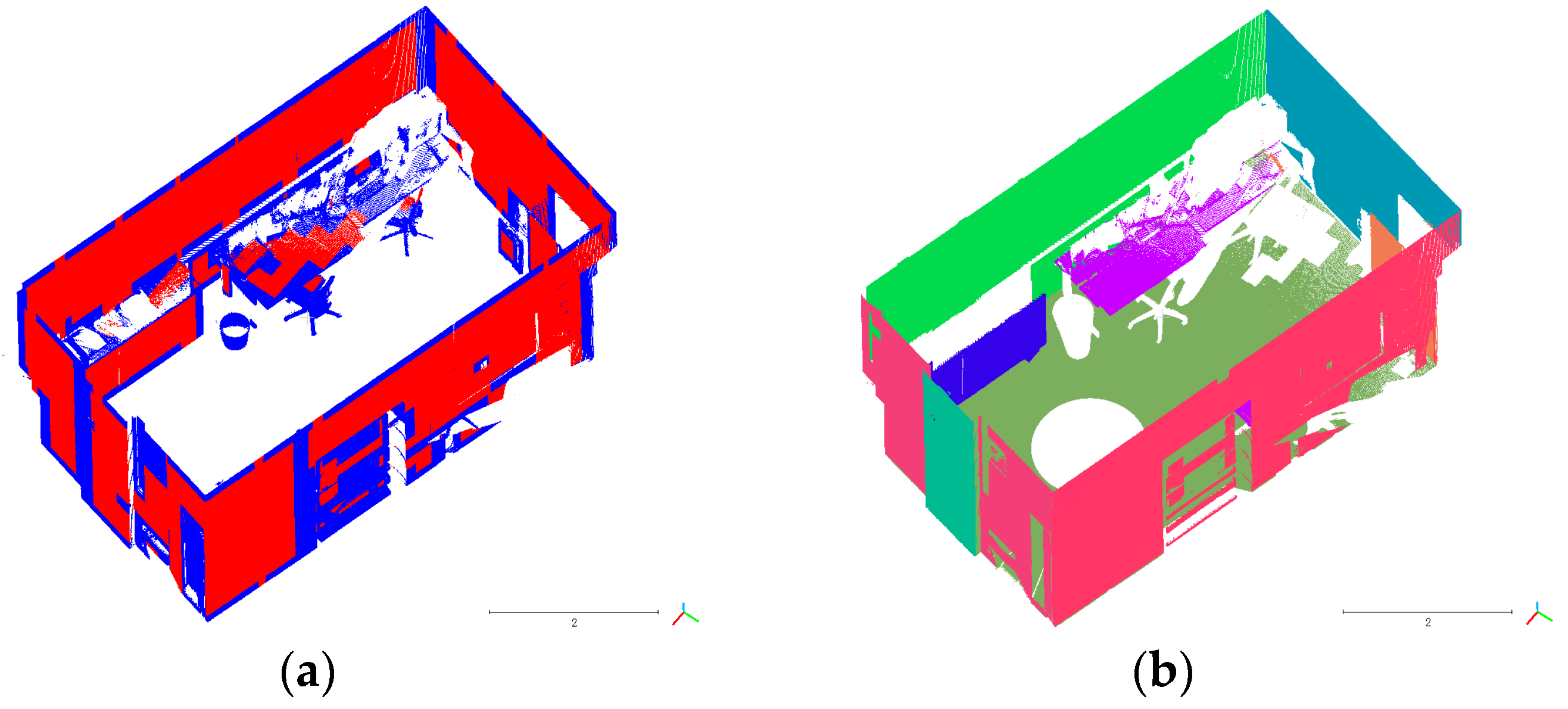
Figure 8.
(a) The NDT cell-classification result for Room-2. The planar and non-planar NDT cells are colored in red and blue, respectively; (b) The NDT-RANSAC plane-segmentation result.
Figure 8.
(a) The NDT cell-classification result for Room-2. The planar and non-planar NDT cells are colored in red and blue, respectively; (b) The NDT-RANSAC plane-segmentation result.

Figure 9.
(a) The NDT cell-classification result for Room-3. The planar and non-planar NDT cells are colored in red and blue, respectively; (b) The NDT-RANSAC plane-segmentation result.
Figure 9.
(a) The NDT cell-classification result for Room-3. The planar and non-planar NDT cells are colored in red and blue, respectively; (b) The NDT-RANSAC plane-segmentation result.
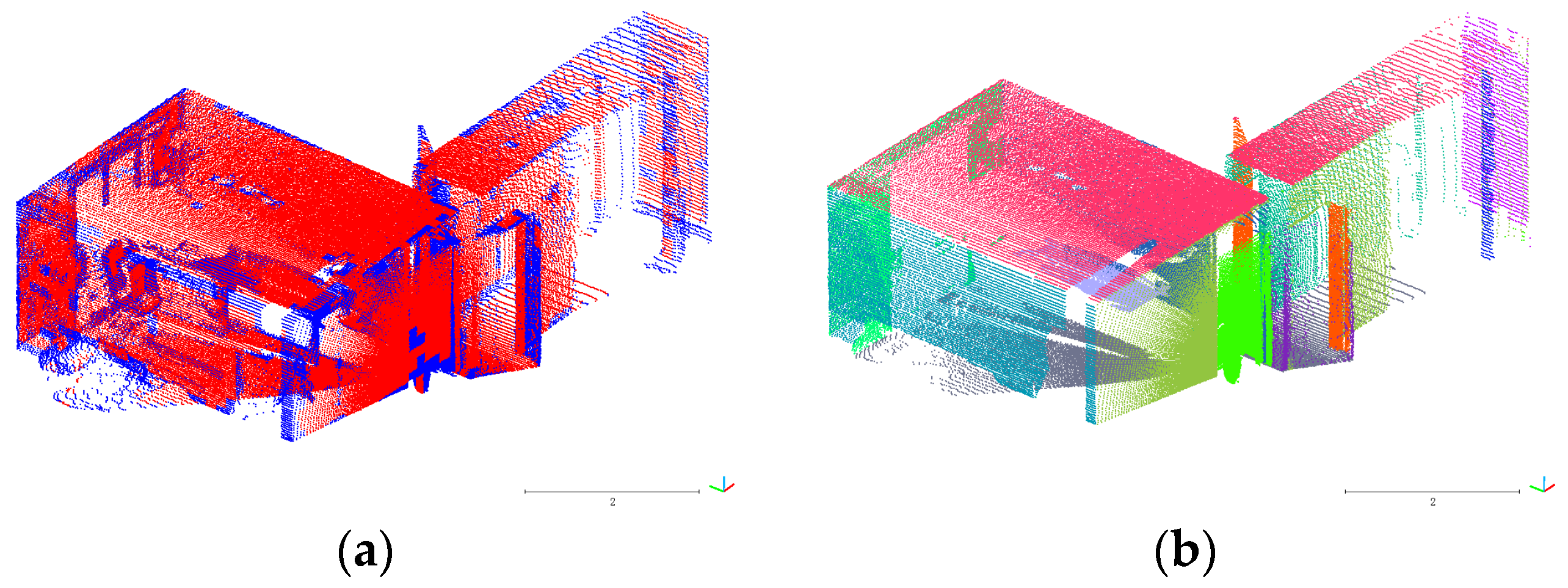
Figure 10.
Plane-segmentation results of RANSAC and NDT-RANSAC evaluated on three datasets. Each figure shows boxplots for four different evaluation metrics—correctness, SR, completeness and quality of plane segmentation. Boxes centered at average values, red line shows median value. (a) Evaluation for Room-1; (b) Evaluation for Room-2; (c) Evaluation for Room-3.


Table 1.
Description of the dataset.
| Test Sites | Length (m) | Width (m) | Height (m) | Points | Average Density (Points/m2) |
|---|---|---|---|---|---|
| Room-1 | 7.0 | 5.4 | 3.2 | 11,050,391 | 91,352 |
| Room-2 | 8.6 | 10.2 | 2.8 | 367,602 | 1486 |
| Room-3 | 7.7 | 9.7 | 2.8 | 367,602 | 1745 |
Table 2.
Percent averages of plane-segmentation results and average computing times on three datasets.
Table 2.
Percent averages of plane-segmentation results and average computing times on three datasets.
| Dataset | Method | Correctness | SR | Completeness | Quality | Time (s) |
|---|---|---|---|---|---|---|
| Room-1 | RANSAC | 37.3% | 62.7% | 52.5% | 26.3% | 333.72 |
| NDT-RANSAC | 98.3% | 0 | 85.0% | 83.8% | 7.43 | |
| Room-2 | RANSAC | 45.9% | 54.1% | 70.1% | 38.3% | 5.57 |
| NDT-RANSAC | 90.4% | 0 | 98.1% | 88.7% | 5.03 | |
| Room-3 | RANSAC | 49.5% | 50.5% | 71.4% | 40.9% | 5.29 |
| NDT-RANSAC | 88.5% | 0 | 94.6% | 84.3% | 2.46 |
© 2017 by the authors. Licensee MDPI, Basel, Switzerland. This article is an open access article distributed under the terms and conditions of the Creative Commons Attribution (CC BY) license (http://creativecommons.org/licenses/by/4.0/).
Share and Cite
MDPI and ACS Style
Li, L.; Yang, F.; Zhu, H.; Li, D.; Li, Y.; Tang, L. An Improved RANSAC for 3D Point Cloud Plane Segmentation Based on Normal Distribution Transformation Cells. Remote Sens. 2017, 9, 433. https://doi.org/10.3390/rs9050433
AMA Style
Li L, Yang F, Zhu H, Li D, Li Y, Tang L. An Improved RANSAC for 3D Point Cloud Plane Segmentation Based on Normal Distribution Transformation Cells. Remote Sensing. 2017; 9(5):433. https://doi.org/10.3390/rs9050433
Chicago/Turabian StyleLi, Lin, Fan Yang, Haihong Zhu, Dalin Li, You Li, and Lei Tang. 2017. "An Improved RANSAC for 3D Point Cloud Plane Segmentation Based on Normal Distribution Transformation Cells" Remote Sensing 9, no. 5: 433. https://doi.org/10.3390/rs9050433
Note that from the first issue of 2016, this journal uses article numbers instead of page numbers. See further details here.