1. Introduction
Shadows exist in most very high resolution (VHR) orthoimagery (with a resolution of up to 1 m) and lead to more complex and detailed land-cover features, especially in urban areas [
1]. Shadow areas usually have incomplete spectral information, lower intensity, and fuzzy boundaries, which seriously affect the subsequent interpretation [
2,
3,
4,
5,
6]. However, dealing with shadows always generates costs in labor and/or time [
7]. Hence, accurate and automatic shadow detection is an active area of research [
8,
9].
Most of the research into shadow detection is based on natural imagery and videos [
10], and relatively few studies have addressed shadow detection in VHR orthoimagery with compound land-cover features and a broader variety of features co-existing in a scene [
11,
12]. The current methods for shadow detection can be divided into three types [
11,
12,
13]: (1) property-based methods [
9,
13,
14,
15,
16,
17,
18,
19,
20]; (2) geometrical methods [
14,
17,
18,
19,
20]; and (3) machine learning methods [
15,
16,
21,
22].
The property-based methods are the most popular approach as the imagery is the only required input. Property-based methods identify shadows using the statistical characteristics of brightness, color, texture, gradient, and edges. In the property-based methods [
23,
24,
25,
26], an initial shadow mask is generated by a thresholding method, among which Otsu’s thresholding method [
27] is the most widely used approach, augmented with various morphological operators. A representative property-based approach deploying invariant color models is Tsai’s spectral method (TSM) [
26], which transforms the red, green, and blue (R-G-B) color images into different invariant color spaces. Otsu’s thresholding method detects the shadowed areas based on the ratio of the hue and intensity components in the image. Based on Tsai’s work, Chung et al. [
25] presented a successive thresholding scheme, instead of a global thresholding process. However, according to Adeline’s survey paper [
11], Tsai’s method performs better than Chung’s algorithm. Liu et al. [
9] used the properties derived from shadow samples to generate a feature space and calculate decision parameters; a series of transformations is then used to separate the shadowed and non-shadowed regions. Using the physical properties of the blackbody radiator model, Makarau et al. [
13] put forward a method based on direct and scattered light having different temperatures. Ngo et al. [
28] applied Otsu’s thresholding method to three binary channels, i.e., C3, ExG, and L. Based on Dempster–Shafer theory, the influence indexes of vegetation and shadow are combined pixel by pixel to improve the detection quality. Markov random fields (MRF) is used to increase the constraint of adjacent pixel information, and the minimum energy method is used to obtain the optimal segmentation result, i.e., shadow areas, vegetation areas, and other areas. Li et al. [
29] employed a matting technique to extract accurate soft shadow masks, with manually identified shadowed and non-shadowed areas as the input. After the manual marking process, the shadow detection performance of Li’s matting method (LMM) is very good. By the use of interactive brushing assisted by a Gaussian mixture model, Xiao et al. [
30] proposed a method to simultaneously detect disconnected shadow areas, with little user interaction.
Geometric methods establish a precise model using a scenario, object, and light source that are not affected by image quality and the material reflectance. These methods require prior knowledge when constructing the model, such as a digital surface model (DSM) and the shoot time of the image. Tolt et al. [
17] proposed a straightforward line-of-sight analysis with a DSM to detect large shadowed and non-shadowed areas, and trained a support vector machine (SVM) supervised classifier with the detected shadow areas to refine the results. Giles [
19] and Steven et al. [
20] proposed similar methods that trace a straight line from every pixel to the solar position at the time of image acquisition, to determine if a topographic obstruction exists between a point on the land surface and the sun. Once the line is obstructed, the pixel is marked as shadow. These two methods require a digital elevation model (DEM), the shoot time, and the coordinates of the scene. A similar idea of judging the coverage of occlusion is described in the work of Aliakbarpour et al. [
31]. Prasath et al. [
32] also applied a similar idea to georeferenced SAR images, and they proposed an automatic method for radar shadow detection from SAR images utilizing geometric projections along with a low-resolution DEM. For a mountainous area, instead of a DEM, Li et al. [
18] applied a DSM, which contains the height of objects, such as building and bridges, to determine the shadows by ray tracing. Khan et al. [
21] employed multiple convolutional deep neural networks (ConvNets) to obtain the most relevant features of the shadows, and fed the learned features to a conditional random field (CRF) model to extract the final shadow mask. Guo et al. [
15] proposed a shadow processing method for natural scenes by segmenting the image with the mean shift algorithm, and estimated the confidence of each region being shadowed by the use of a trained classifier. A soft matting technique is then applied to produce smooth shadow boundaries. Lorenzi et al. [
16] selected samples of shadowed and non-shadowed counterparts from different regions as initial values, which are fed into the classifier to obtain a binary shadow mask.
Unfortunately, many of the shadow detection methods based on natural scenes fail when processing complex remote sensing images. Compared to natural images, remote sensing images have a larger range, as more shadows exist in a scene and they contain more complex features. Hence, significant problems are encountered when automatically detecting shadows in VHR remote sensing images [
33]. High-accuracy detection results are essential in the final shadow compensation process. However, in the current methods, there is a tradeoff between accuracy and automaticity [
26]. Penumbras do not appear in low-resolution images, and thus penumbra detection is seldom applied [
29]. However, in VHR images, this should be considered as the width of the penumbra can be more than five pixels, which can seriously affect the compensation accuracy in the final output. Moreover, the property-based methods, in general, are not independent of the data in the image. Therefore, these methods are only applicable to images obtained under certain conditions, and they may fail on images obtained at different times and under varying atmospheric conditions. For shadowed and non-shadowed areas having similar attribute information, such as low-brightness non-shadows (e.g., dark asphalt on roads and black roofs) and high-brightness shadowed regions (e.g., windows), or bluish objects (e.g., water), misjudgment often occurs [
26,
34]. A robust automatic matching method for shadowed areas and the corresponding non-shadowed areas in VHR imagery begs further research [
7].
The geometrical methods are independent of the quality of the remote sensing images and the material reflectance. However, obtaining a priori information has been a major hindrance to the development of the geometric methods. Fortunately, automatic 3D photogrammetry software, such as Acute3D, Pix4D, etc., now provides a richer and more reliable foundation for the application of geometrical methods. In this paper, a simple and effective automatic shadow detection method for complex urban environments is presented, which combines the advantages of the property-based and geometrical methods. The sun position and a DSM are required to rebuild the geometric relationship between the surface and the sun at the time the raw images were captured, thereby obtaining a coarse binary shadow mask. The next step is to process the mask and determine the initial labels for the shadowed and non-shadowed areas using morphological operators, and refine the shadow areas with the matting algorithm. Since all the procedures are processed directly from the input data, the proposed method can be performed on VHR orthoimagery with few preset parameters. In the experimental part, using manually delineated ground-truth data, the proposed method is compared with two state-of-the-art methods. The shadow removal results in three types and scales of shadow situations confirm that the performance of the proposed method is better than the other two methods, from both visual and quantitative aspects.
The rest of the paper is organized as follows.
Section 2 details the proposed shadow detection method.
Section 3 provides the experimental results and analysis for different resolutions of VHR images.
Section 4 analyzes the possible error sources of the proposed method.
Section 5 describes the considerations in the process of parameter selection.
Section 6 concludes the paper.
2. The Proposed Shadow Detection Method
Most of the high-accuracy shadow detection methods require the samples of shadows and their corresponding non-shadowed areas to be manually collected before the process of detection, and most of the automatic methods fail on certain shadow-like features, such as water and dark asphalt roads [
26,
29,
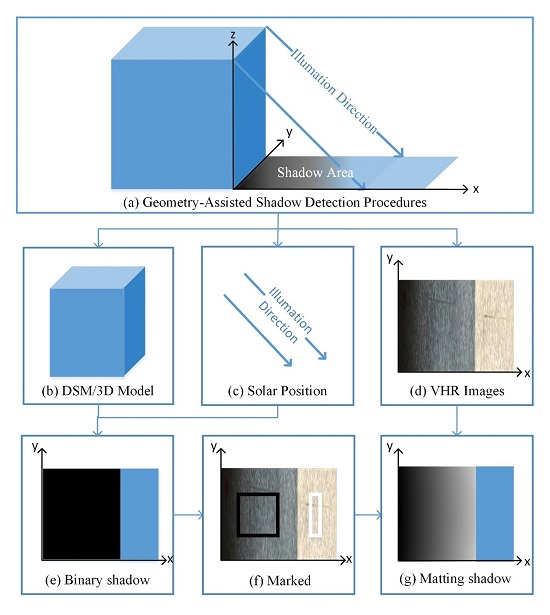
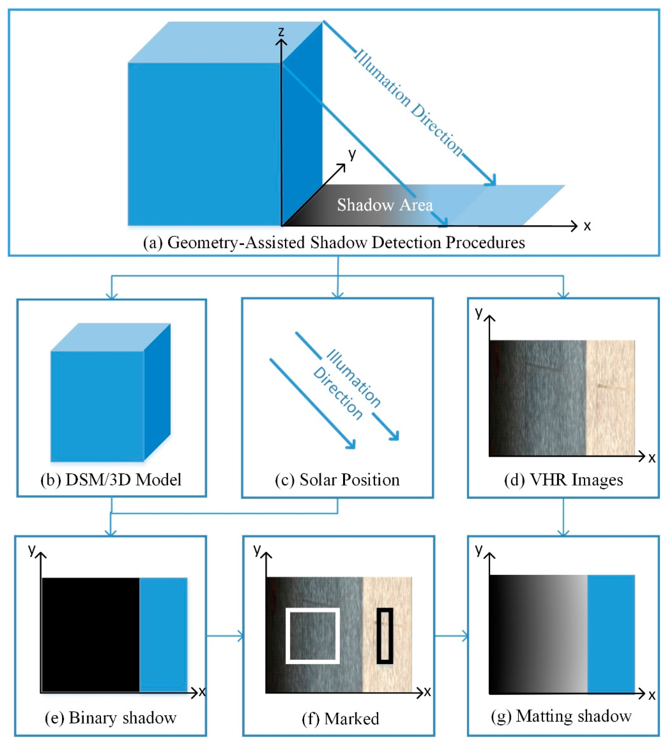
33]. The proposed method is processed in three steps and benefits from the automation of the spectral-based methods and the high accuracy of the geometric methods. The procedure of the proposed geometry-assisted shadow detection method is shown in
Figure 1.
The geometrical model of the proposed method (
Figure 1a) is composed of a DSM/3D model (
Figure 1b), the solar position (
Figure 1c), and the VHR images (
Figure 1d). With the input of the DSM and the solar position, the geometrical methods are largely automated, and can produce highly accurate results when identifying shadows (as shown in
Figure 1e). This is the first step, which is described in detail in
Section 2.1. Due to the technical limits of DSM production at the current time, DSMs usually have a slightly lower horizontal accuracy at building boundaries than VHR imagery. In addition, DSMs may include some processing artifacts caused by moving cars, trees, and water, which can cause shadow detection failure [
18]. To overcome this drawback, a matting method is used in the third step.
Interactive digital matting is an accurate method that can be applied to extract shadowed areas in handheld camera pictures or remote sensing imagery of a small area. Compared to natural imagery, VHR remote sensing imagery has a lower feature resolution and a much larger range, which results in the shadowed areas being smaller and more fragmented. Marking all the shadowed and non-shadowed areas in VHR images manually, as in the matting method of Li et al. [
29] (LMM), would incur significant time costs. Meanwhile, directly applying a matting method on these images may fail because this does not distinguish the shadowed and non-shadowed areas in sufficient detail. In the proposed method, to balance the time and labor, every shadowed and non-shadowed area in the image is delineated with a single mark, which is assisted by morphological erosion and skeleton processing. This is the second step of the proposed method, which is described in detail in
Section 2.2. After the morphological processing, the proposed method delineates the shadowed/non-shadowed areas automatically with a shadow mask generated by the geometric method. As shown in
Figure 1f, the white and black lines represent the marks of the shadowed and non-shadowed areas, respectively.
Figure 1g shows that the marks are then fed into the matting machine, and a final soft shadow mask with high accuracy and low time cost is obtained. This is the final step of the proposed method, which is discussed in
Section 2.3.
2.1. Geometrical Shadow Detection
The first step is to produce a binary shadow mask (
Figure 1e) from the DSM/3D model (
Figure 1b) and the solar position (
Figure 1c). Based on the assumption that the sun is a parallel light source, the sunlight is traced by the solar elevation and azimuth, which are calculated by the shoot time and the geographic coordinates of the imagery.
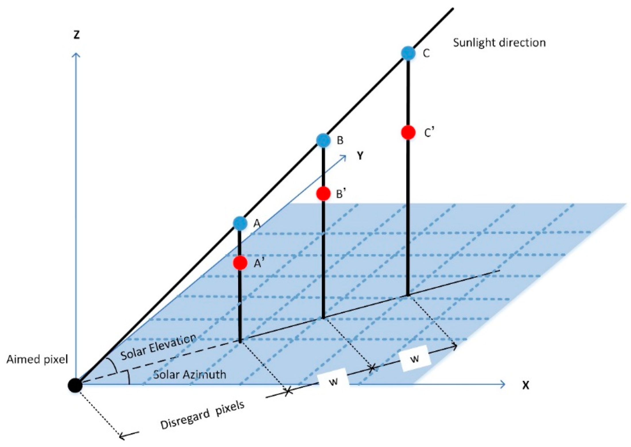
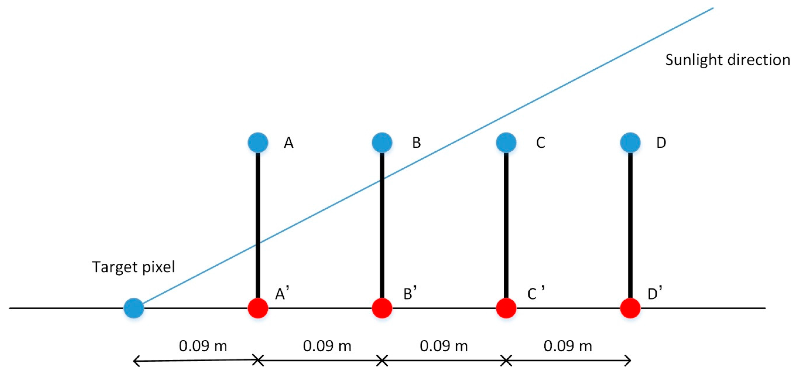
As shown in
Figure 2, we draw a line from the target pixel to the sun, and calculate the interpolated elevation values (blue points) for the pixels the line passes through. The width w is calculated (as shown in Equation (1)) based on the grid width of the DSM that is recorded in the header file of the data and the solar azimuth angle. A three-dimensional view of
Figure 2 is shown in
Figure 3.
We then compare the height of the real elevation values (red points) and the interpolated elevation values (blue points) in the order of distance from the current pixel (in the order of A, B, C, as shown in
Figure 2 and
Figure 3) and we disregard a certain number of pixels (equivalent to a 1-m ground distance) closest to the current pixel to reduce noise such as DSM elevation errors (the error sources are discussed in
Section 4). Detailed notes on parameter selection are provided in
Section 5.1. Once the real elevation is above the interpolated elevation (in the case of B and B’ in
Figure 2a), we stop the cycle and assign the target pixel as a shadowed pixel (the black point in
Figure 2a); otherwise, we assign the target pixel as a non-shadowed pixel (the white point in
Figure 2b). Through calculating the pixels one by one, a binary shadow mask is obtained.
2.2. Mask Processing with Morphological Operators
Before obtains a finer shadow mask, representative marks of every shadowed/non-shadowed area are required. An automatic way to obtain the required marks is introduced in this step, which corresponds to the process shown in
Figure 1e,f. As the boundary of the original binary shadow mask is not as reliable as the center, the mask is further processed to obtain purer marks, using an erosion operation with a 10-by-10 “circle” structuring element to eliminate noisy and inaccurate boundaries (the parameter selection is detailed in
Section 5.2).
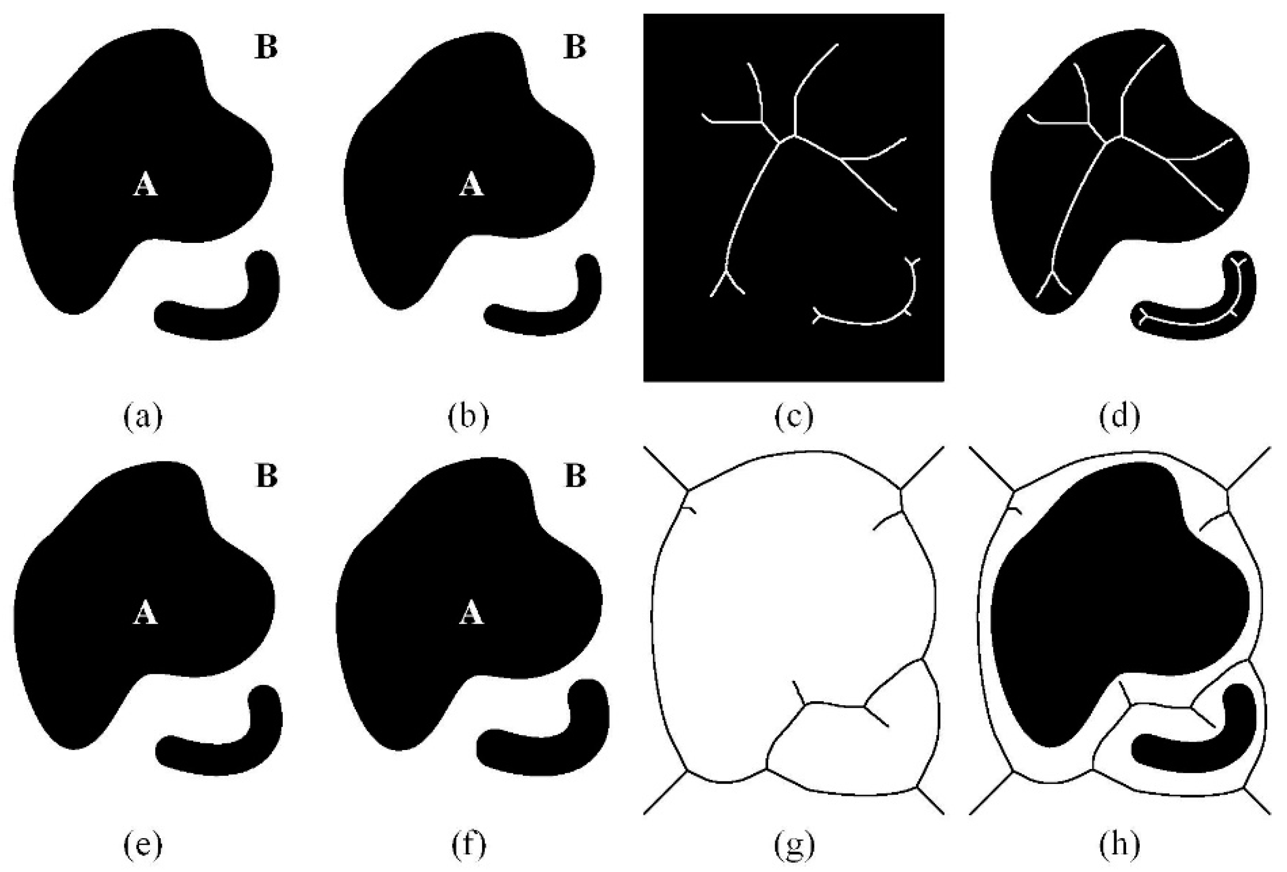
As shown in
Figure 4, areas A and B are exemplary non-convex boundary shapes, which are representations of the complex shapes in the shadow results, such as lakes, or trees on a street. The erosion operation is used to “erase” the inaccurate boundaries of the shadowed areas (as shown in
Figure 4a,b). A similar procedure is used to yield candidate non-shadowed areas (as shown in
Figure 4d,e). Every candidate black/white pixel in
Figure 4b,e indicates a region of shadowed/non-shadowed area. This step is designed to select representative pixels of each region for faster matting processing. By applying a skeleton operation, a linear shadowed/non-shadowed area delineation is derived. The skeleton operation can remove pixels on the boundaries of areas, but does not allow areas to break apart. Overlaying the shadowed/non-shadowed skeleton (the white/black lines in
Figure 4c,f) on the raw image, we obtained the input image to be used in the next step. This operation preserves the key shape characteristics for the matting and greatly decreases the computational cost of the matting.
2.3. Shadow Matting
Interactive digital matting is an accurate way to extract areas of interest in imagery. In a matting method, an image
is considered to be composed of a foreground image
and a background image
. Note that, in the proposed case, the foreground image
is equivalent to the shadowed areas, and the background image
represents the non-shadowed areas. Based on the proposed shadow delineation method, accurate shadow regions are extracted as the foreground objects from the image, where
stands for the probability of each pixel belonging to absolute shadow, ranging from 0 to 1. We briefly describe the process below. Detailed notes on parameter selection and the proof of the theorem can be found in Levin’s article [
35,
36].
The linear combination of the foreground and background is undertaken as follows:
where
denote the values of
at pixel
. Assuming
F and
B are constant over a small window around each pixel, then Equation (2) can be rewritten as:
where
, and
is a small image window, which we set as
in our experiments. This relation suggests finding
and
by minimizing the following cost function:
where
is a small image window around pixel
, and
is the weight of the regularization term on
. According to Theorem 1 in [
35]:
where
L is an
matrix, whose
th element is:
where
is the Kronecker delta,
is the number of pixels in this window,
is a
mean vector of the colors in the window
,
is a
covariance matrix, and
is a
identity matrix.
To extract the final mask
, matching the shadowed/non-shadowed constraints that we obtained in
Section 2.2, we minimize the following energy function, which is firstly proposed by Levin [
35], and a final shadow mask is obtained.
where
is a diagonal matrix whose diagonal elements are 1 for the marked pixels (as described in
Section 2.2) and 0 for the others, and
is the vector containing the specified
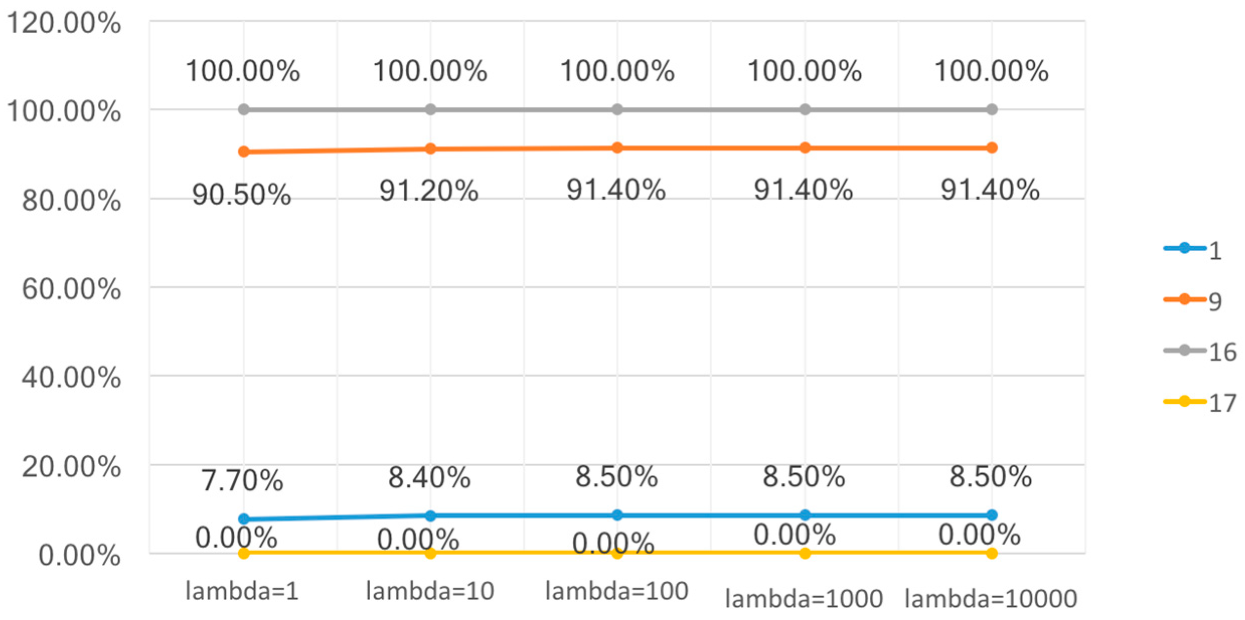
values for the marked pixels, and 0 for the others. Parameter
is usually set as a large number, and we followed the value Levin used in [
35], i.e., 100. The influence of
is discussed in detail in
Section 5.3.
The former item
is to ensure that
is under the assumption that the background (non-shadowed areas) and foreground (shadowed areas) are locally smooth in a small window around each pixel. The usage of the latter item
is to add the influence of the marked pixels to the final results, which constrains the differences between the marked
(0 or 1) and the final
(ranging from 0 to 1) to be as small as possible. The initial value of
for the constrained pixels is 0, and the values of the others are not. The final
values of the constrained pixels may be very close or equal to the corresponding
, and for the other pixels, they vary from 0 to 1. As the cost is quadratic in
, the global minimum can be solved by differentiating and setting the derivatives to 0, which is equal to solving the sparse linear system as follows:
With the three steps illustrated above, the final soft shadow mask
is obtained. The values in
represent the probabilities of belonging to absolute shadow. The experimental results of the proposed method and two state-of-the-art methods (TSM [
26] and LMM [
27]) are discussed in the next section.
3. Experiments and Comparisons
The proposed method was implemented on a personal computer with an Intel Core i5-2500K 3.3 GHz CPU, using MATLAB in the Windows 7 environment. Two state-of-the-art methods, as proposed in [
26,
27], were also implemented for comparison and evaluation. As
Table 1 shows, TSM is used as a representative of the automatic spectral-based shadow detection approach [
11,
26], and LMM is applied as it is both accurate and representative of the matting methods using manually delineated shadowed and non-shadowed areas [
27]. The results of LMM and the proposed method are judged as soft shadow in the matting process, which means that the value of each pixel in the shadow result ranges from 0 to 1, instead of 0 or 1 in the binary shadow result. For a comparison and evaluation of the methods, an effective thresholding method is needed to convert the soft shadow into a binary shadow. In our tests, Otsu’s thresholding method was applied to automatically obtain the suitable threshold value and the binary shadow mask.
The data used in the experiments are shown in
Table 2. In test 1, the data were composed of a 0.25 m DSM generated from Trimble Inpho 5.3 software and a 0.25-m orthophoto computed by Trimble Inpho OrthoVista from aerial imagery of an urban area of Vaihingen, Germany [
37]. The data in test 2 were a 0.09 m DSM acquired from aerial airborne laser scanning (ALS) and a 0.09 m orthophoto computed by Trimble INPHO OrthoVista from aerial imagery of an urban area of Vaihingen. Data of tests 1 and 2 were provided by the German Society of Photogrammetry, Remote Sensing and Geoinformation (DGPF) project [
38]. The solar elevation/azimuth was 41°/107°. The data used in test 3 were from a 0.06 m orthophoto and a 0.06 m DSM processed by Pix4D of an urban area of Zurich, Switzerland. The raw aerial images were provided by the ISPRS/EuroSDR project. The solar elevation/azimuth was 55°/195°, respectively.
The data in the test 1 images contained water features, which are often incorrectly detected by the current automatic shadow detection methods [
26]. The images of test 2 contained the common urban features, such as shadows from concentrated high-rise buildings and trees. The test 3 images contained the common urban features such as roads, buildings, and trees.
The three bands of the optical imagery were NIR, red, and green in order in tests 1 and 2, and red, green, and blue in test 3. As the bands of the imagery in tests 1 and 2 were NIR-R-G, the plants in both
Section 3.1 and
Section 3.2 are shown in red. The experimental results of the three methods working on the R-G-B channels are shown in
Section 3.3. Three sets of images were used to test the accuracy and performance of the three approaches on different sources and different scales of data.
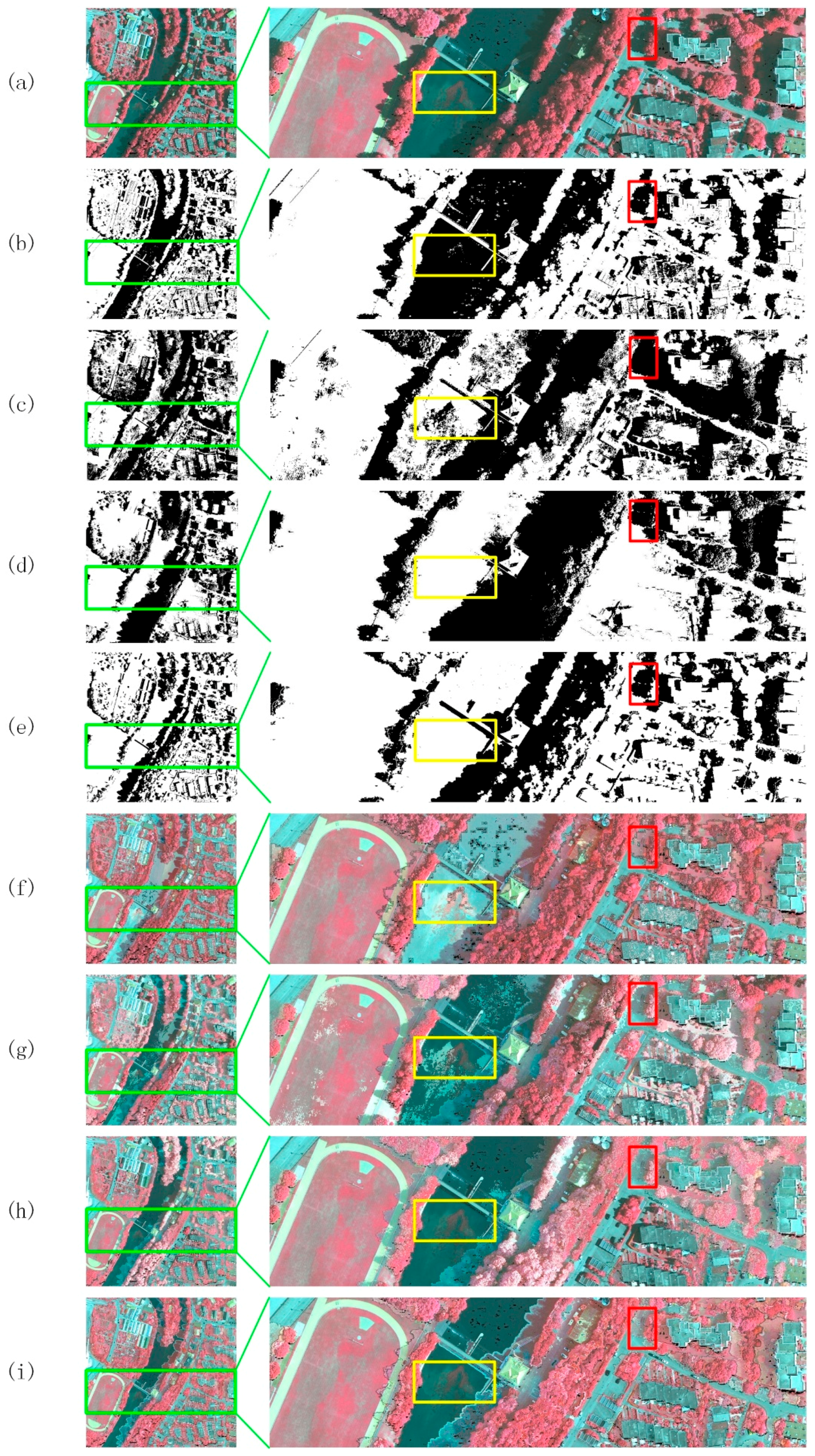
3.1. Water Areas
Figure 5a shows the original imagery of test 1. In this test, the main challenge for the shadow detection methods is the river. Water has a lower intensity and bluish color, which is similar to the characteristics of shadows. As shown in the yellow box in
Figure 5b (result of TSM), water causes false detection for the automatic spectral-based shadow detection methods.
Figure 5c shows the shadow detection result of LMM. With manually delineated shadowed and non-shadowed areas, the shadow boundaries in the result of LMM are similar to those in the original imagery.
Figure 5d shows the result of the proposed method, where it can be seen that most of the shadows are correctly detected. However, there are still some problems. For example, some of the wooded areas are falsely discerned as shadow, and some small building shadows are miss-detected.
Figure 5e shows the manually selected shadow mask, which is considered as the true shadow on the ground. Using the shadow compensation method described in [
26],
Figure 5f–i shows the results obtained with the shadow masks displayed in
Figure 5b–e. The right images in
Figure 5 are zoomed images of the region within the green boxes of the left images.
To empirically compare the effects of the different methods, four well-known metrics—producer’s accuracy, user’s accuracy, overall accuracy and F-score—are used to evaluate the shadow detection results [
11,
39]. As mentioned at the beginning of this section, an automatic thresholding method (Otsu’s thresholding method [
27]) is applied on the soft shadow mask to obtain a binary value. The metrics are defined as follows.
The producer’s accuracy is used to measure how accurately the method detects the true shadowed and non-shadowed pixels.
where
represents the producer’s accuracy of the shadowed pixels and
represents the non-shadowed pixels. The true positive (TP) is the number of shadowed pixels correctly discerned when compared to the manually selected mask, and true negative (TN) is the number of non-shadowed pixels that are correctly detected and identified by the true values from the manual mask. False negative (FN) is the number of true shadow pixels judged as non-shadowed, and false positive (FP) is the number of non-shadowed pixels that are falsely detected as true shadow pixels.
The user’s accuracy is used to indicate the probability of the correctness of the detected shadowed and non-shadowed pixels.
where
represents the user’s accuracy of the shadowed pixels and
represents the non-shadowed pixels.
The overall accuracy
refers to the percentage of correctly detected shadowed and non-shadowed pixels.
The F-score is a balanced way to judge the user’s accuracy and the producer’s accuracy.
The accuracy measurements are shown in
Table 3, where the bold numbers represent the highest values and the underlined numbers represent the lowest. From the table, it can be seen that TSM obtains an acceptable producer’s accuracy performance for
(82.0%) and a user’s accuracy for
of 65.8%. This method, however, delivers the worst performance in producer’s accuracy performance for
(83.3%) and user’s accuracy for
(92.2%). LMM obtains an acceptable producer’s accuracy for
(86.2%) and user’s accuracy for
(92.6%), and the worst producer’s accuracy for
(71.7%) and user’s accuracy for
(55.9%). The proposed method obtains the best performance for all the six metrics. The producer’s accuracy for
is 89.7%, the producer’s accuracy for
is 82.2%, the user’s accuracy for
is 67.7%, and the user’s accuracy for
is 95.0%. For the overall accuracy, the proposed method obtains a value of 84.4%, TSM ranks second at 82.4%, and LMM obtains an acceptable value of 75.9%. For the F-score, the proposed method ranks first with 77.1%, TSM ranks second with 73.5%, and LMM obtains 67.8%.
From the zoomed images in
Figure 5, it can be seen that the river is falsely detected as shadow by TSM and LMM in
Figure 5b,c, whereas the proposed method correctly judges it as non-shadow (
Figure 5d). Thus, the proposed method has an outstanding advantage in detecting shadows in areas with water when compared to the other two methods. To verify the effect of the shadow masks in the shadow removal, the shadow removal method proposed in [
26] and the five indicators proposed in [
40] are used to analyze the shadow removal results of the three methods.
The shadow removal method in [
26] was carried out by matching the cumulative distribution function (CDF) of the shadowed pixels and their surrounding non-shadowed pixels. From the red boxes in the upper right part of the zoomed images in
Figure 5f–h, it can be seen that the shadow area near the trees is correctly discerned as shadow by all three methods, but the compensation results are quite different. The result of TSM is the worst of the three, and it falsely discerns cement as trees. Both the results of LMM and the proposed method display an improved spectral quality for the objects in the red boxes. Overall, the proposed method performs the best of the three methods in the visual interpretation.
Table 4 shows the statistics of the five indicators of mean, standard deviation, entropy, gradient, and hue deviation index (HDI) [
40]. The first four indicators are commonly used in the evaluation process. Detailed descriptions of them can be found in Shen’s paper [
40]. The HDI is used to measure the variance of hue between the original image and the processed image, which is calculated as follows:
where
represents the hue value of the pixel located at
from the original image, and
represents the hue value of the same pixel from the processed image.
and
are the size of the image.
In
Table 4, the three numbers in each cell represent the values of the three channels (IR-R-G for tests 1 and 2, R-G-B for test 3). The mean intensities of the image processed by the three methods are all increased, which is due to the removal of the dark shadow areas. At the same time, the three methods have very close results in standard deviations, meaning that the contrast of the entire image is lower than the original imagery. Information entropy denotes the information richness of the image; the higher the better. All the methods yield good results, with almost the same information entropy values as the original image. The gradient refers to the detail contrast in the image. All three methods enhance the detail contrast, which may be caused by the features under the shadow. An HDI of less than 1% means that the shadow removal process can effectively preserve the hue.
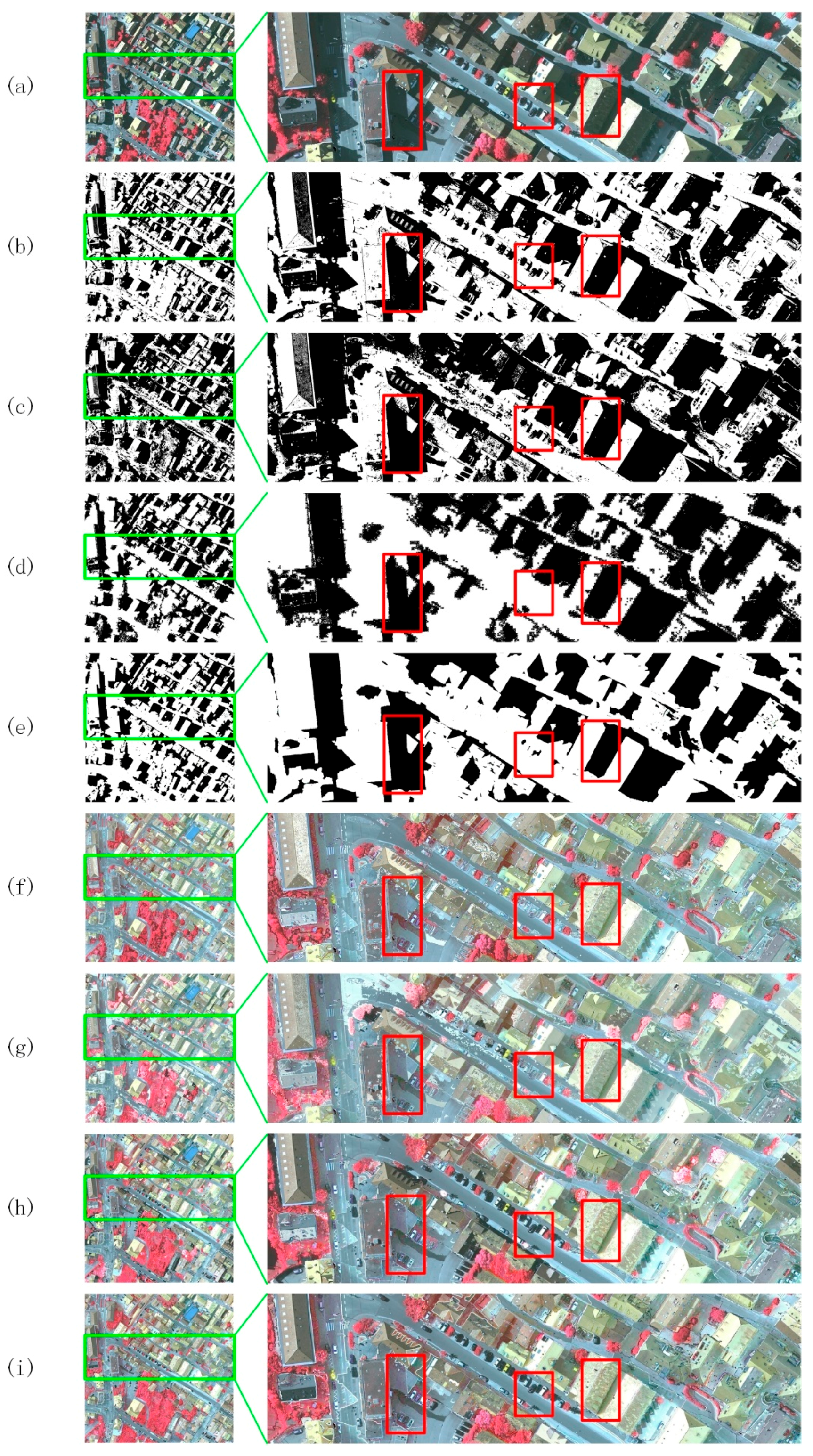
3.2. City Center Areas
In test 2, an area in the center of Vaihingen was selected, which contained the common features found in urban areas, such as crowded buildings, trees, and cars.
Figure 6a shows the original image. The shadow detection results of TSM, LMM, and the proposed method are respectively shown in
Figure 6b–d.
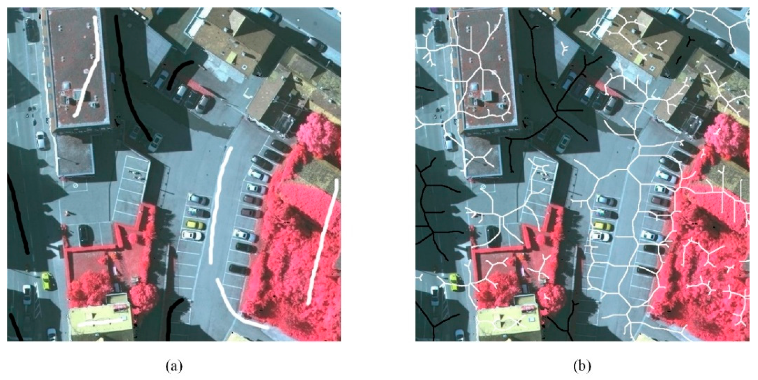
Figure 6b displays false detection of dark objects, where cars and other artifacts are incorrectly identified as shadowed areas. As the buildings in the scene have complex roofs, manually delineating the shadowed and non-shadowed areas is a very time-consuming process. The delineation for the shadowed/non-shadowed areas in
Figure 6c,d is shown in
Figure 7a,b. In
Figure 7a, the shadowed and non-shadowed areas of every building are manually delineated. The results shown in
Figure 6c may not be accurate enough, and thus a finer delineation of the shadowed and non-shadowed areas is needed. According to [
29], a finer delineation can lead to a more accurate shadow mask. Many buildings exist in an image of a city center, but a single mark for each shadowed and non-shadowed area for each building is sufficient in the proposed method.
Figure 6d shows the automatically generated result of the proposed method, which contains less noise and clearly represents the shadowed/non-shadowed areas, obtained without any human input.
Figure 6e shows the manually delineated shadow mask.
Figure 6f–i shows the compensated results obtained using the shadow compensation method described in
Section 3.1, with the shadow masks displayed in
Figure 6b–e. The right images in
Figure 6 are zoomed images of the region within the green boxes of the left images.
The accuracy evaluation is shown in
Table 5, where TSM ranks second in the user’s accuracy and the producer’s accuracy. LMM obtains the best performance for two out of the six metrics, with a producer’s accuracy for
of 96.7% and a user’s accuracy for
of 97.1%. At the same time, LMM delivers the worst producer’s accuracy for
of 66.9% and user’s accuracy for
of 63.3%. The proposed method obtains the best score in producer’s accuracy for
of 93.0%, user’s accuracy for
of 87.9%, and an acceptable performance in terms of producer’s accuracy for
with a score of 87.3%. The user’s accuracy for
ranks third, 4.6% lower than the best result. In terms of overall accuracy, TSM obtains a value of 91.2%, the proposed method ranks second at 90.5%, and LMM obtains an acceptable score of 77.9%. For the F-score, TSM ranks first with 88.6%, the proposed method ranks second with 87.5%, and LMM obtains 76.5%.
According to the statistics shown in
Table 6, the mean intensity and the standard deviation values for the three methods show the same tendencies as the results in
Table 4 for test 1. For the information entropy, the proposed method delivers the best result of the three methods. All three methods enhance the detail contrast, with low HDI values. Compared to
Table 4, the overall trend between the results of test 2 and test 1 is almost unchanged.
For the visual interpretation, the red boxes in
Figure 6f–h show the compensation results of the shadow masks of the three methods. As the shadow mask of TSM is hard shadow (binary shadow mask), the ground is overcompensated in the left red box in
Figure 6b, and the black cars are falsely compensated, as shown in the middle red box in
Figure 6b. With limited manual delineation, the compensation result of LMM misses some shadowed areas, such as the objects in the two red boxes shown in
Figure 6e. From the three red boxes shown in
Figure 6h, the proposed method accurately detects the shadows of the buildings, without being influenced by the cars and artifacts, obtaining a more stable and balanced shadow removal performance than the other two methods.
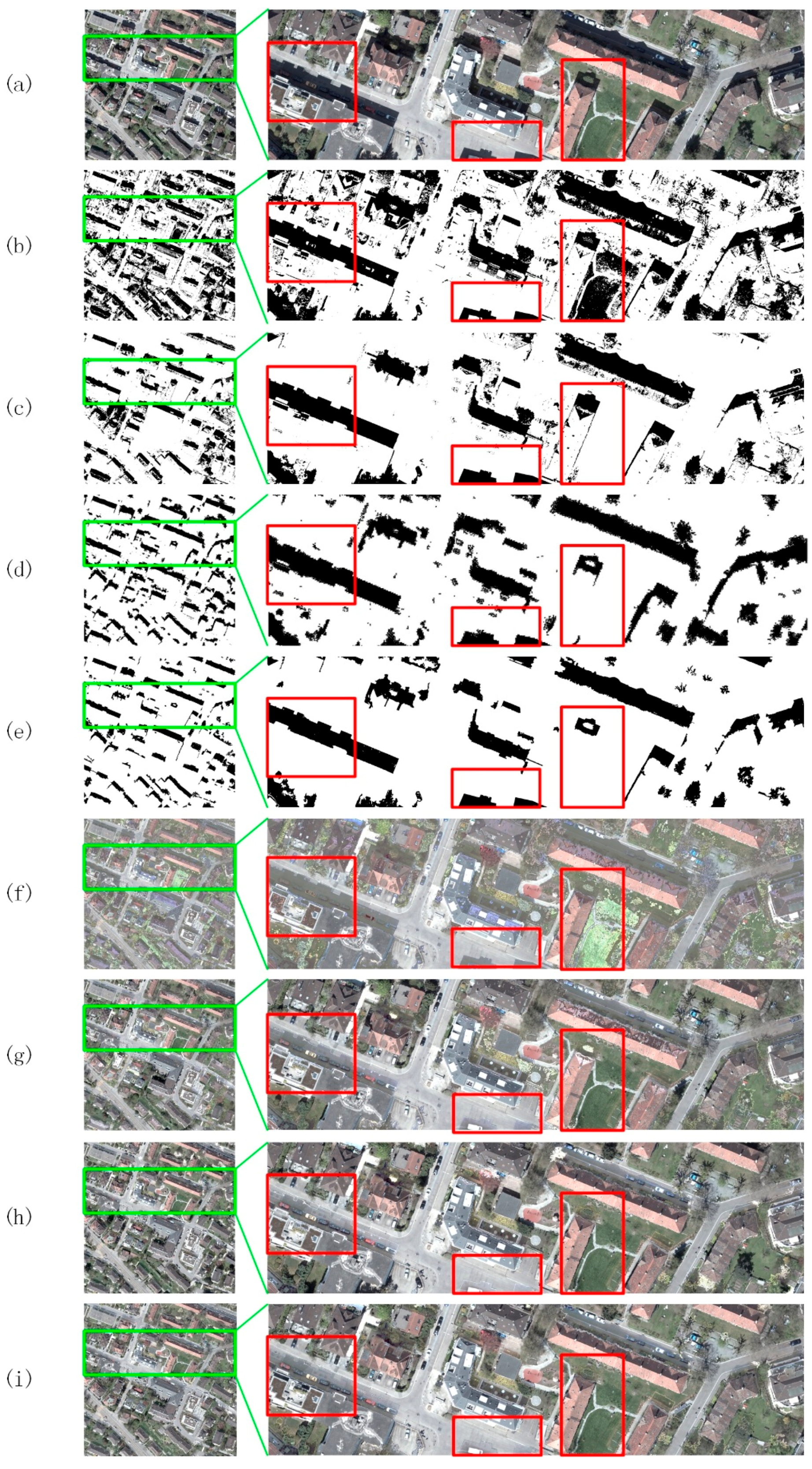
3.3. RGB Orthophotos
The test region in test 3 was an urban area of Zurich, which also contained the common urban features such as buildings, roads, parks, and cars.
Figure 8a shows the original image. The shadow detection results of TSM, LMM, and the proposed method are respectively shown in
Figure 8b,d.
Figure 8b displays false detection, with trees, cars, and other artifacts incorrectly identified as shadowed areas. The results shown in
Figure 8c contain a lot of noise.
Figure 8d shows the automatically generated result of the proposed method, which shows a clear representation for the shadowed/non-shadowed areas, and fewer undetected shadows for the small areas, obtained without any human input.
Figure 8e shows the manually delineated shadow mask.
Figure 8f–i shows the compensated results obtained using the shadow compensation method described in
Section 3.1 and
Section 3.2, with the shadow masks displayed in
Figure 8b–e. The right images in
Figure 8 are zoomed images of the region within the green boxes of the left images.
The accuracy evaluation is shown in
Table 7, where TSM obtains the best performance for the producer’s accuracy for τ
s of 96.3% and user’s accuracy for σ
n of 99.0%. At the same time, TSM delivers the worst producer’s accuracy for τ
n with 76.8%, and a user’s accuracy for σ
s of 46.6%. LMM ranks second in the user’s accuracy and the producer’s accuracy. The proposed method obtains the best score in the producer’s accuracy for τ
n with 94.7%, user’s accuracy for
with 74.4%, and an acceptable performance in terms of user’s accuracy for
with a score of 95.2%. The producer’s accuracy for
ranks third. In terms of overall accuracy, the proposed method ranks first at 91.6%, LMM obtains an acceptable score of 91.2%, and TSM obtains a value of 80.0%. For the F-score, the proposed method ranks first at 80.0%, LMM obtains a value of 76.6%, and TSM obtains a value of 61.9%.


