
Development of Geospatial and Temporal Characteristics for Hispaniola’s Lake Azuei and Enriquillo Using Landsat Imagery

Abstract
:
1. Introduction
2. Materials and Methods
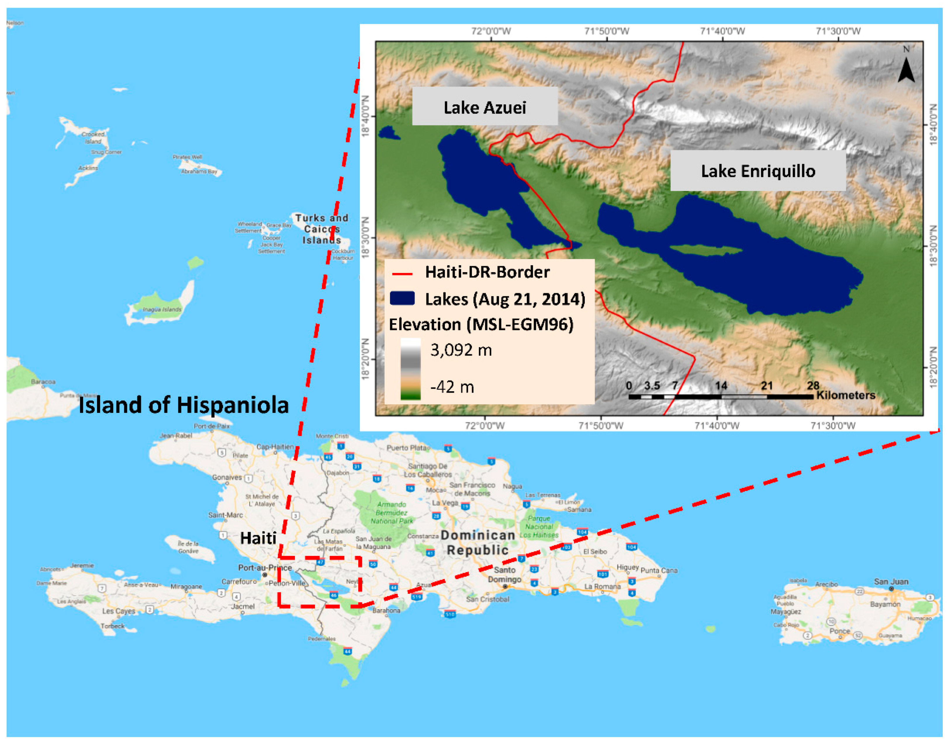
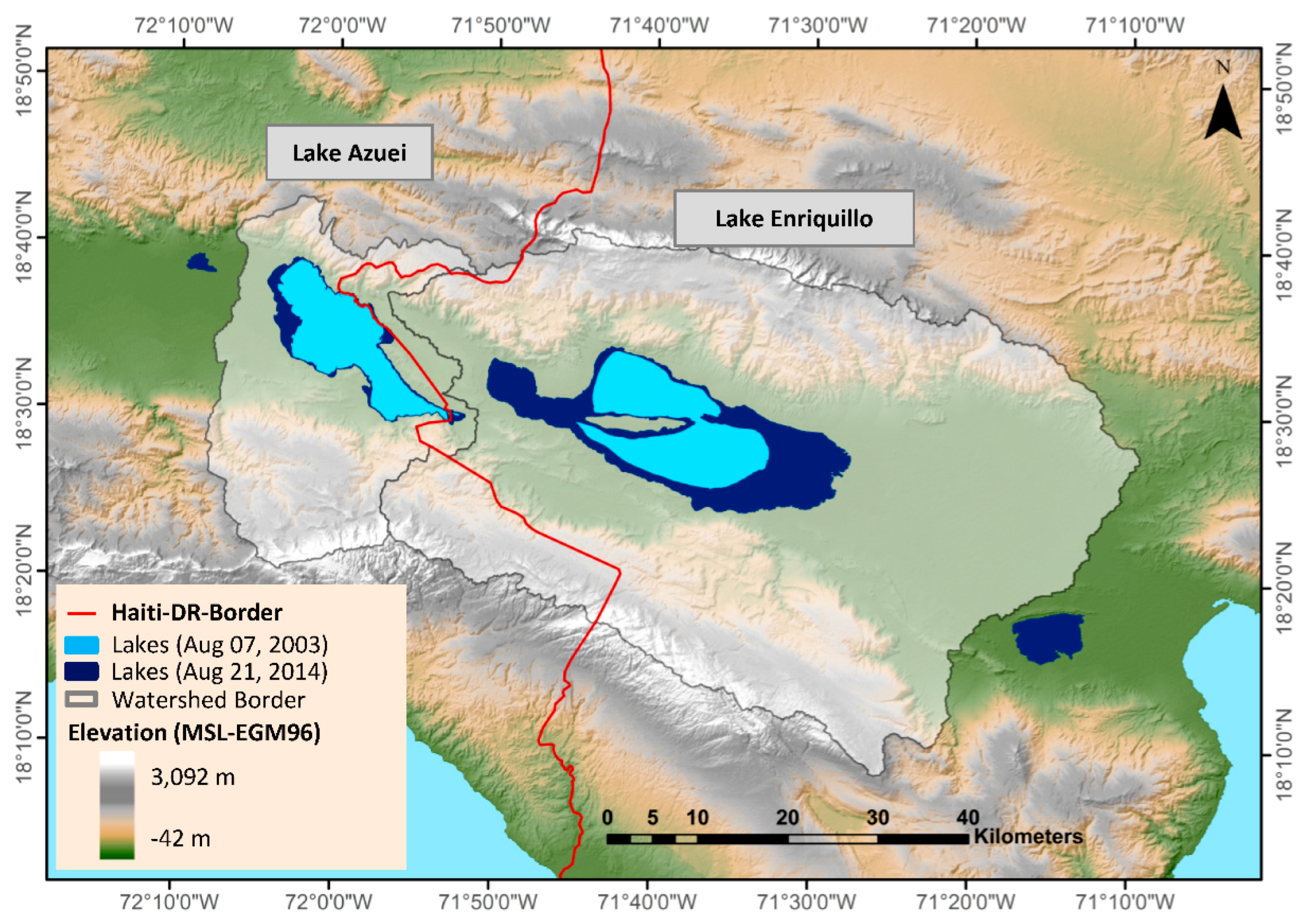
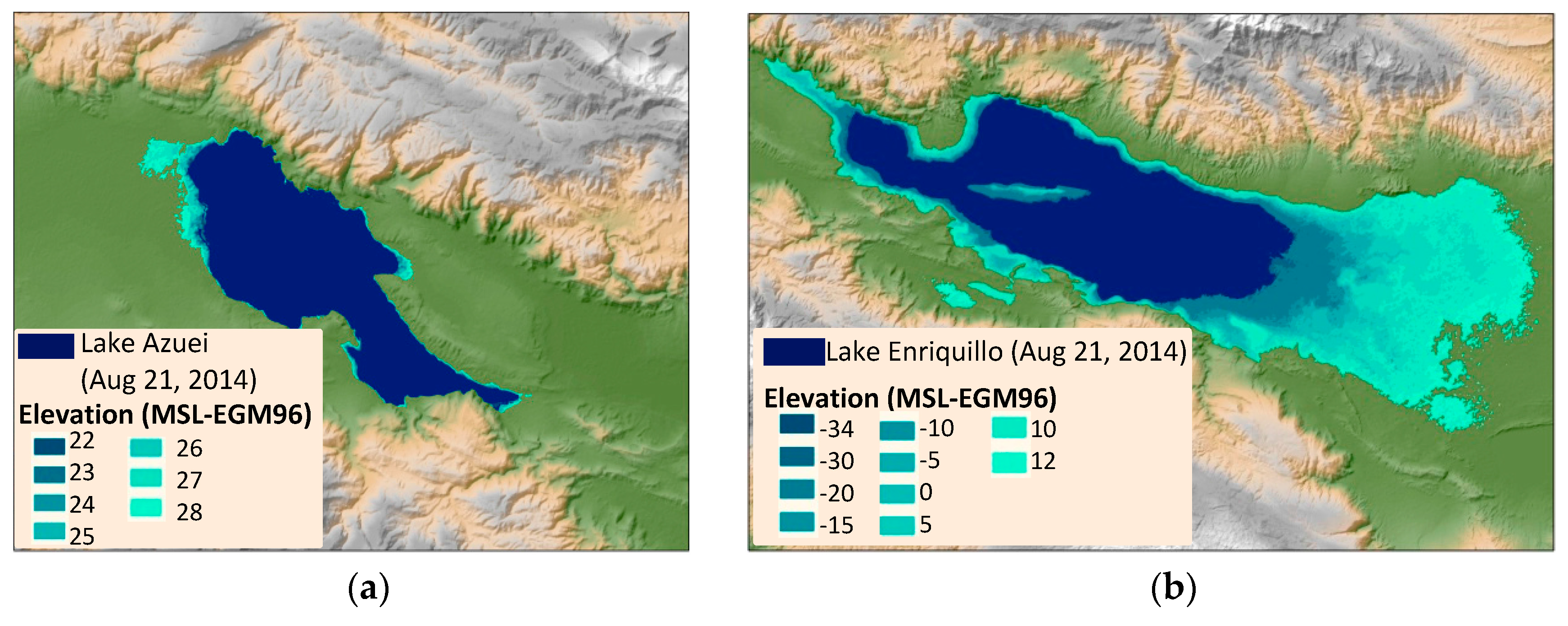
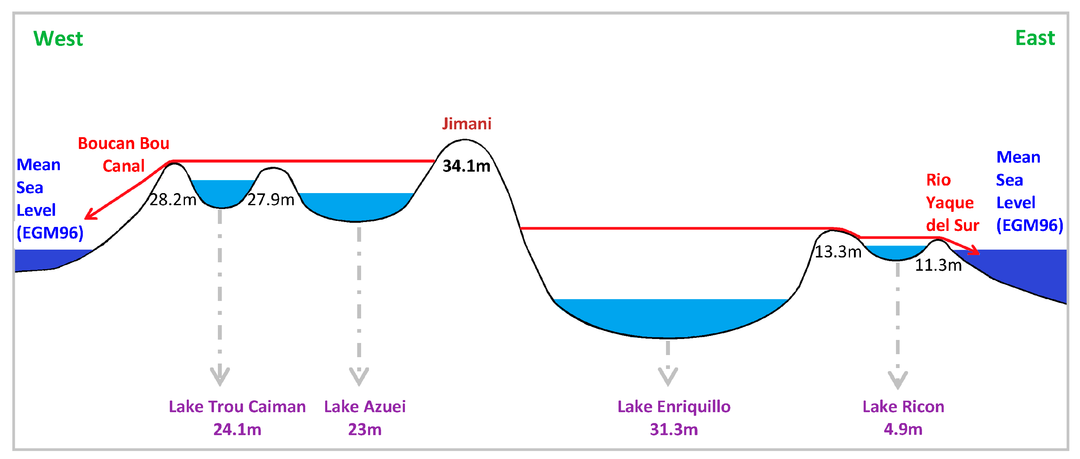
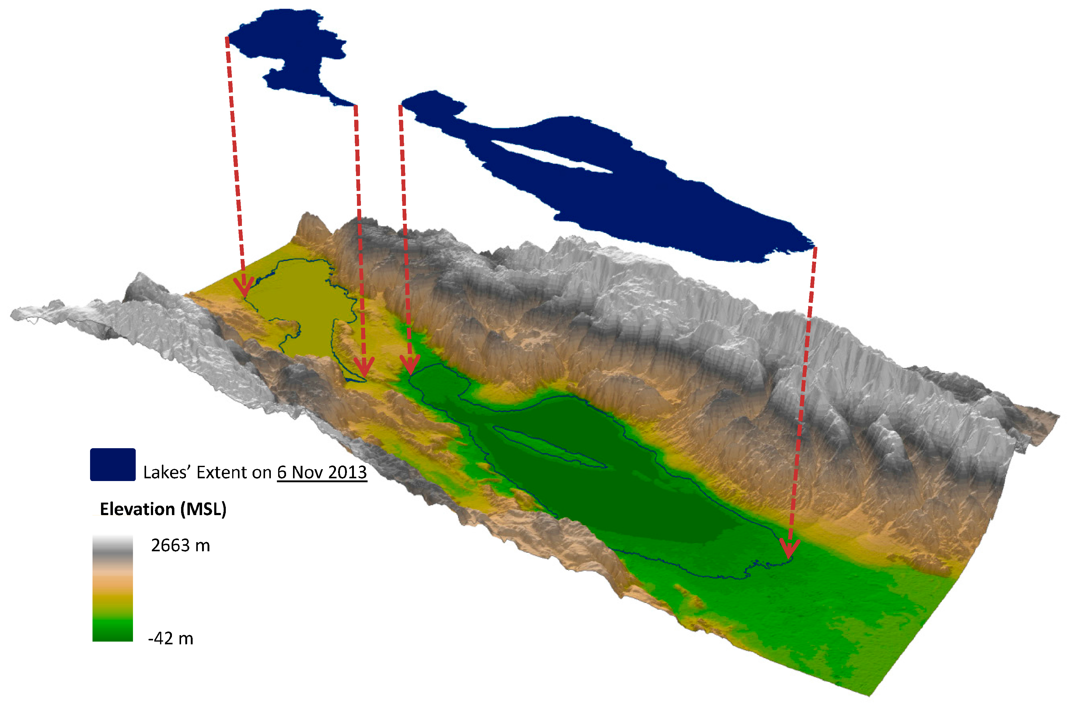
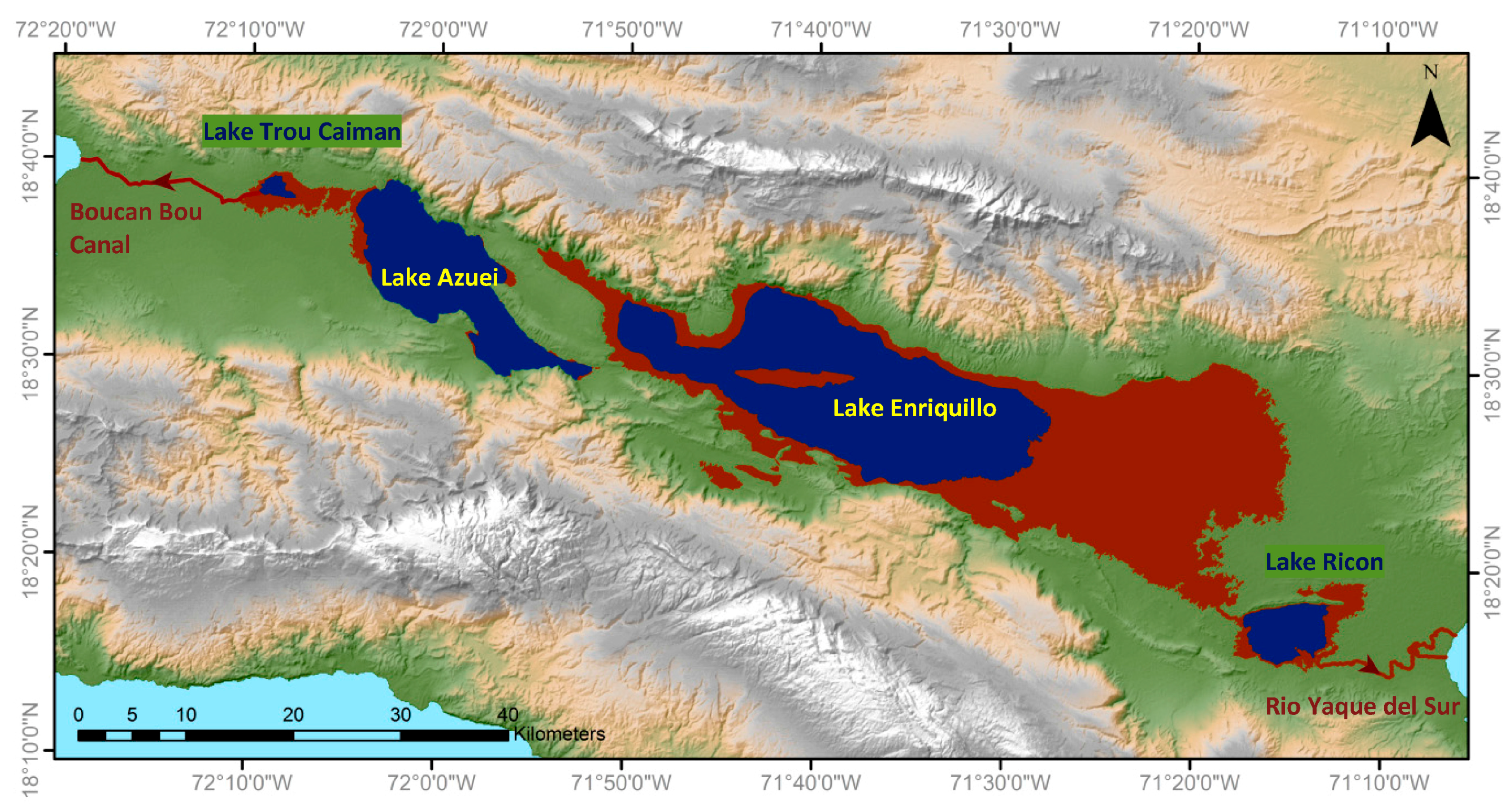
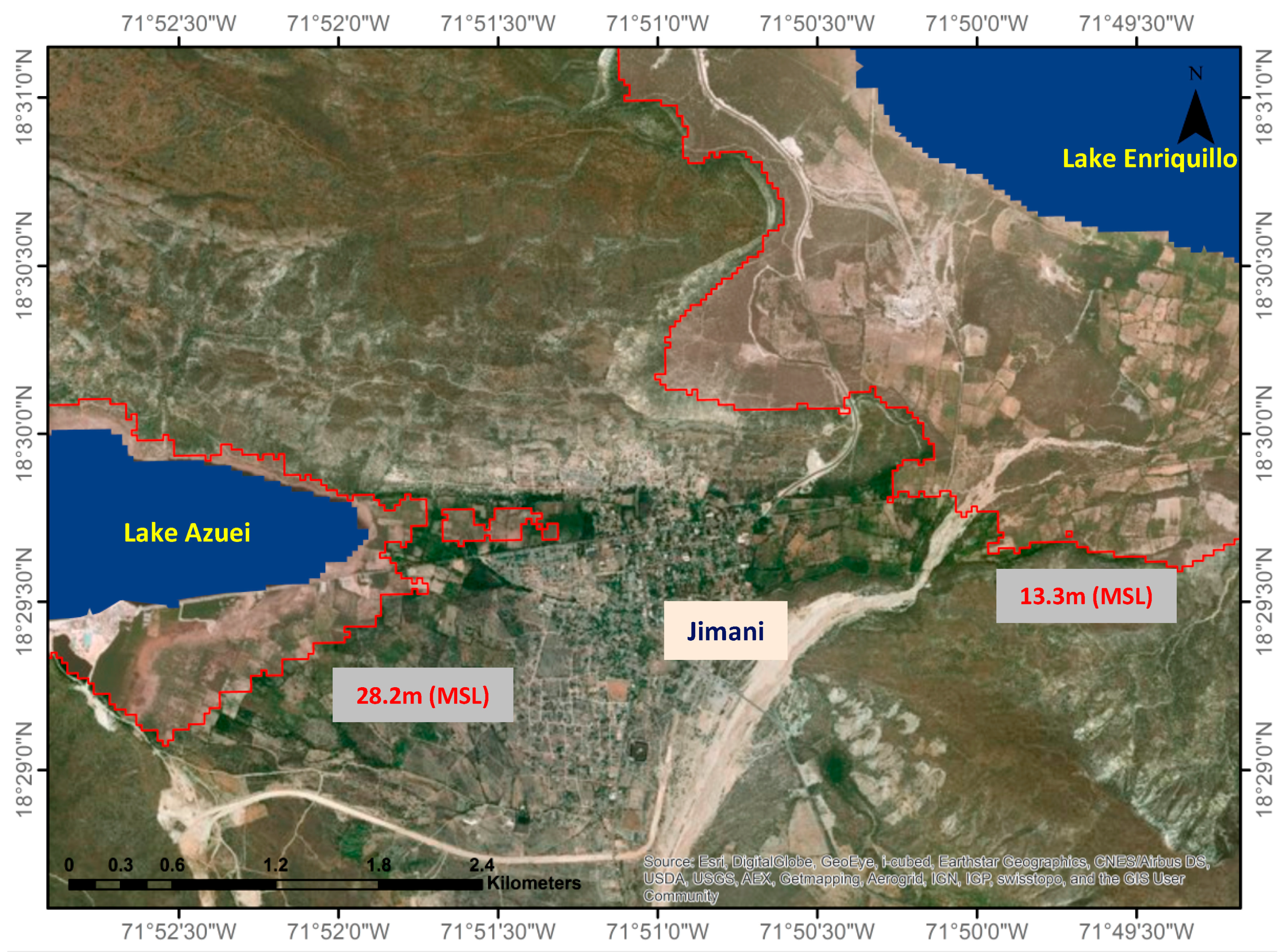
2.1. Study Area
2.2. Landsat Imagery Acquisition and Preprocessing
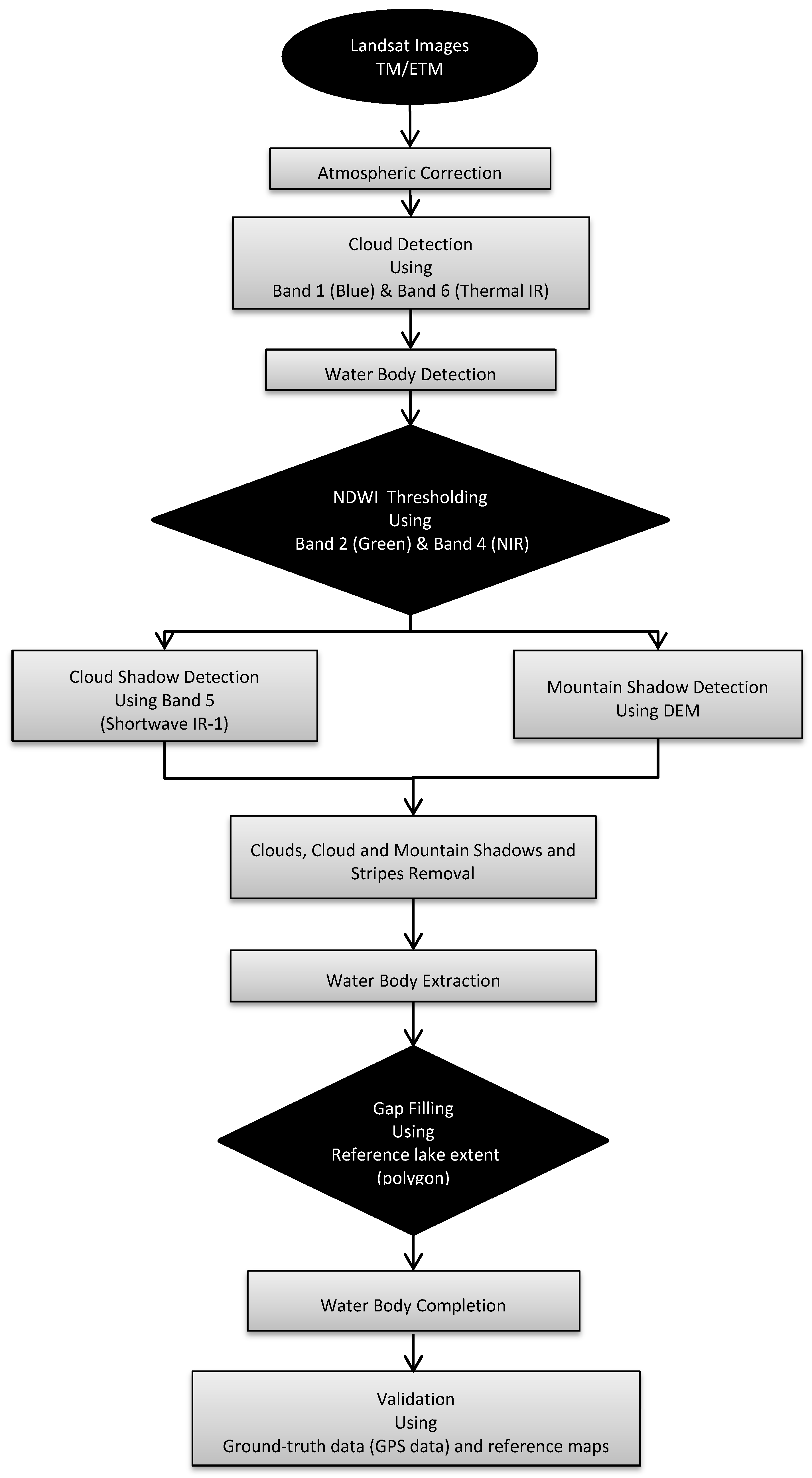
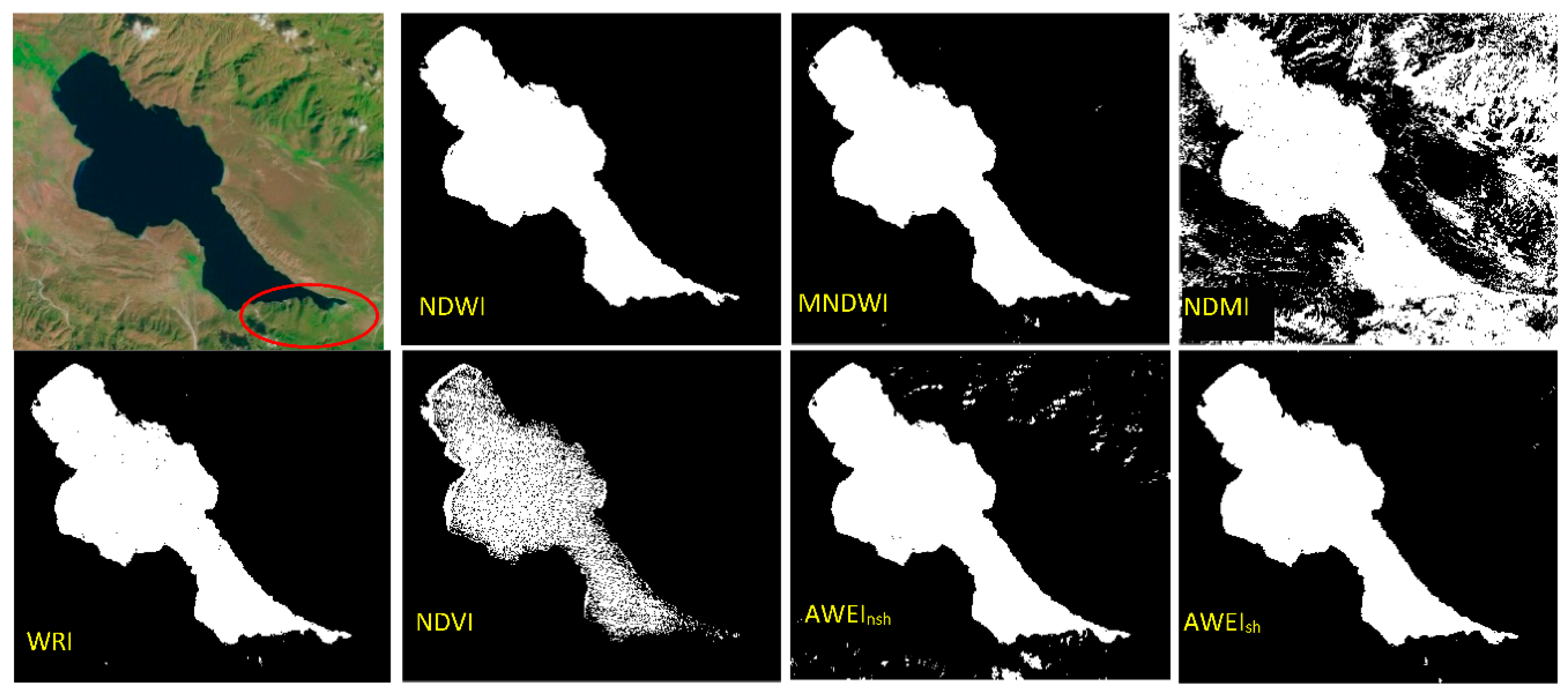
2.3. Water Body Extraction
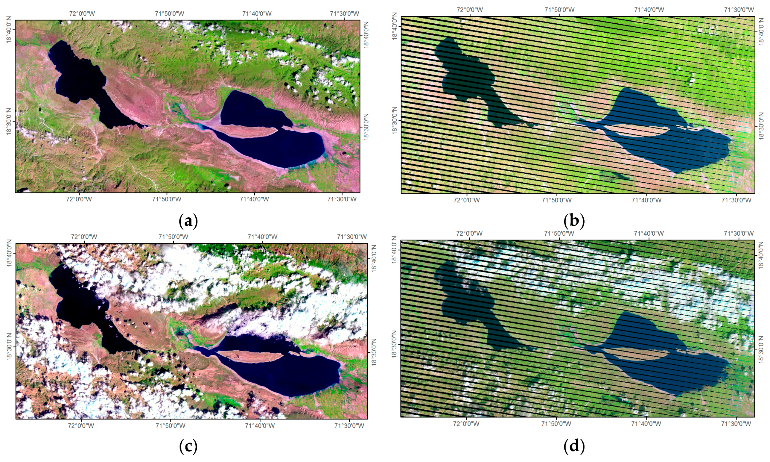
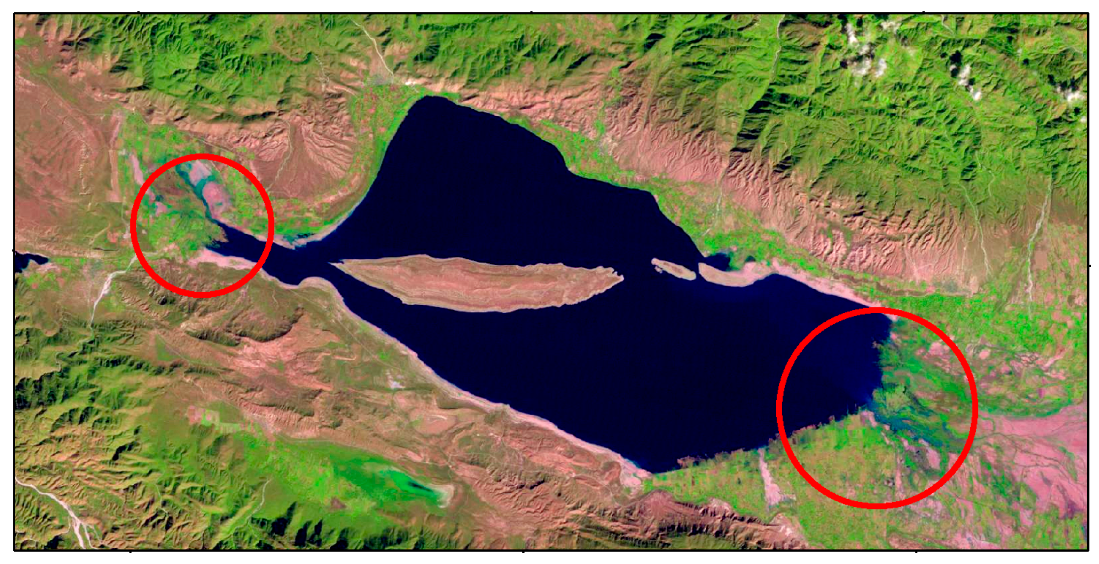
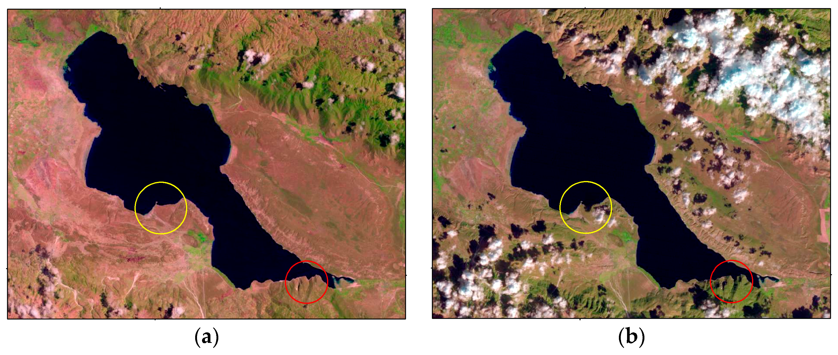
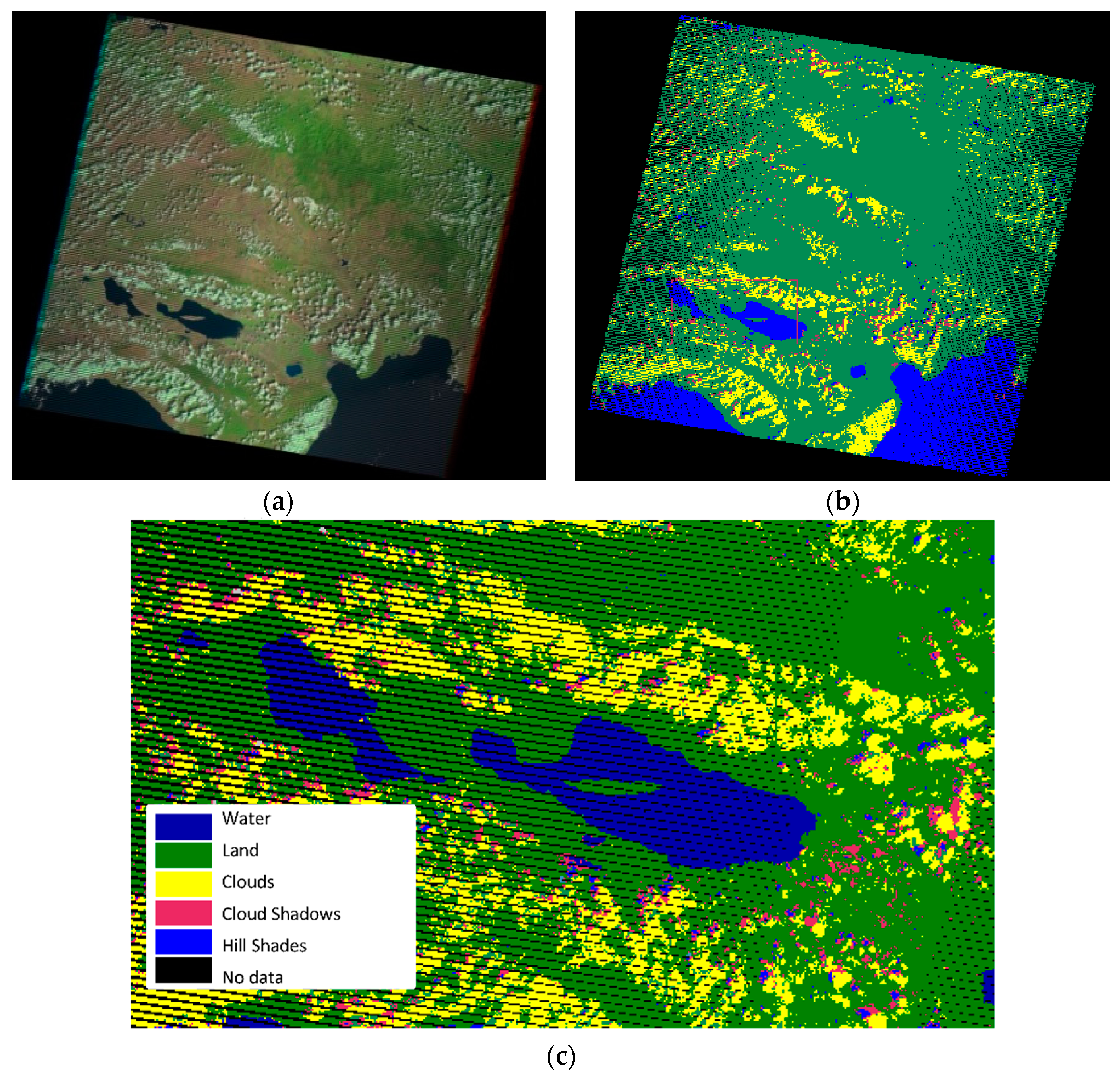
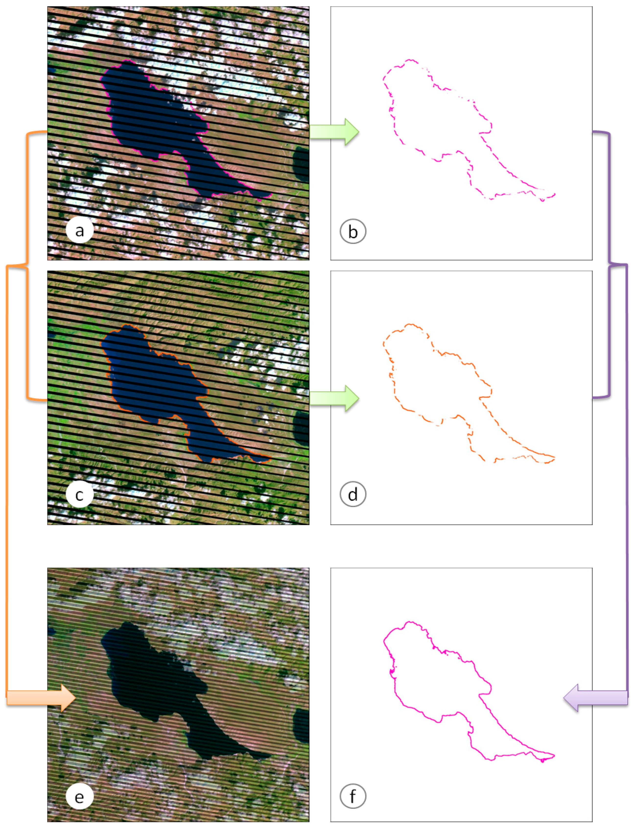
2.4. Cloud and Shadow Detection
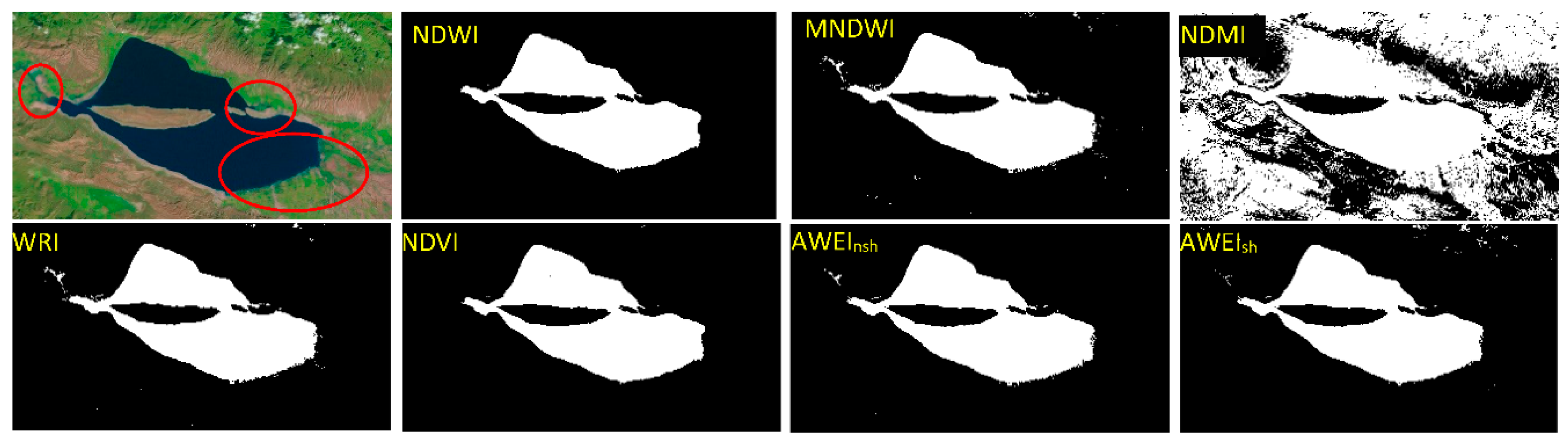
2.4.1. Water Indices
2.4.2. Gap Filling
2.4.3. Final Algorithm
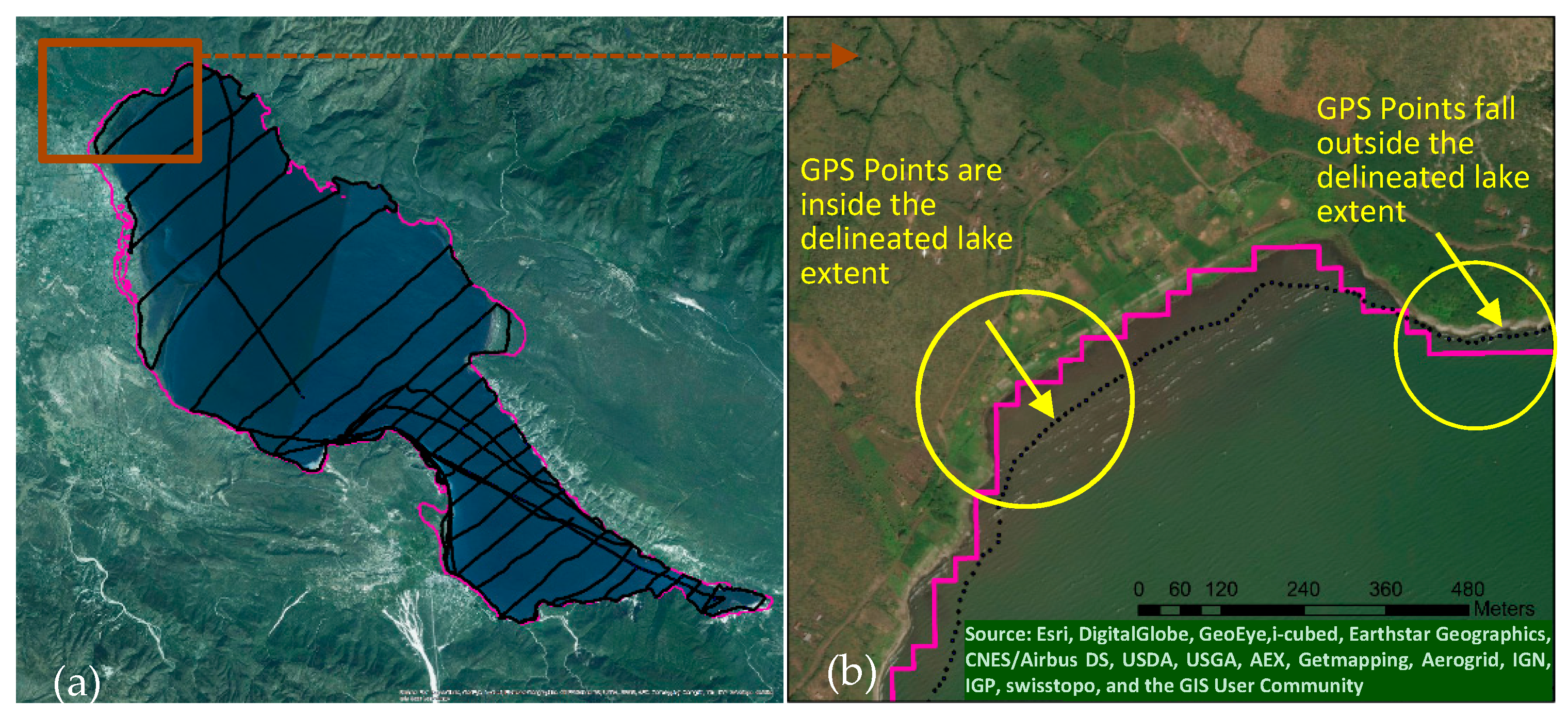
2.5. Validation of Image Analyses
3. Results
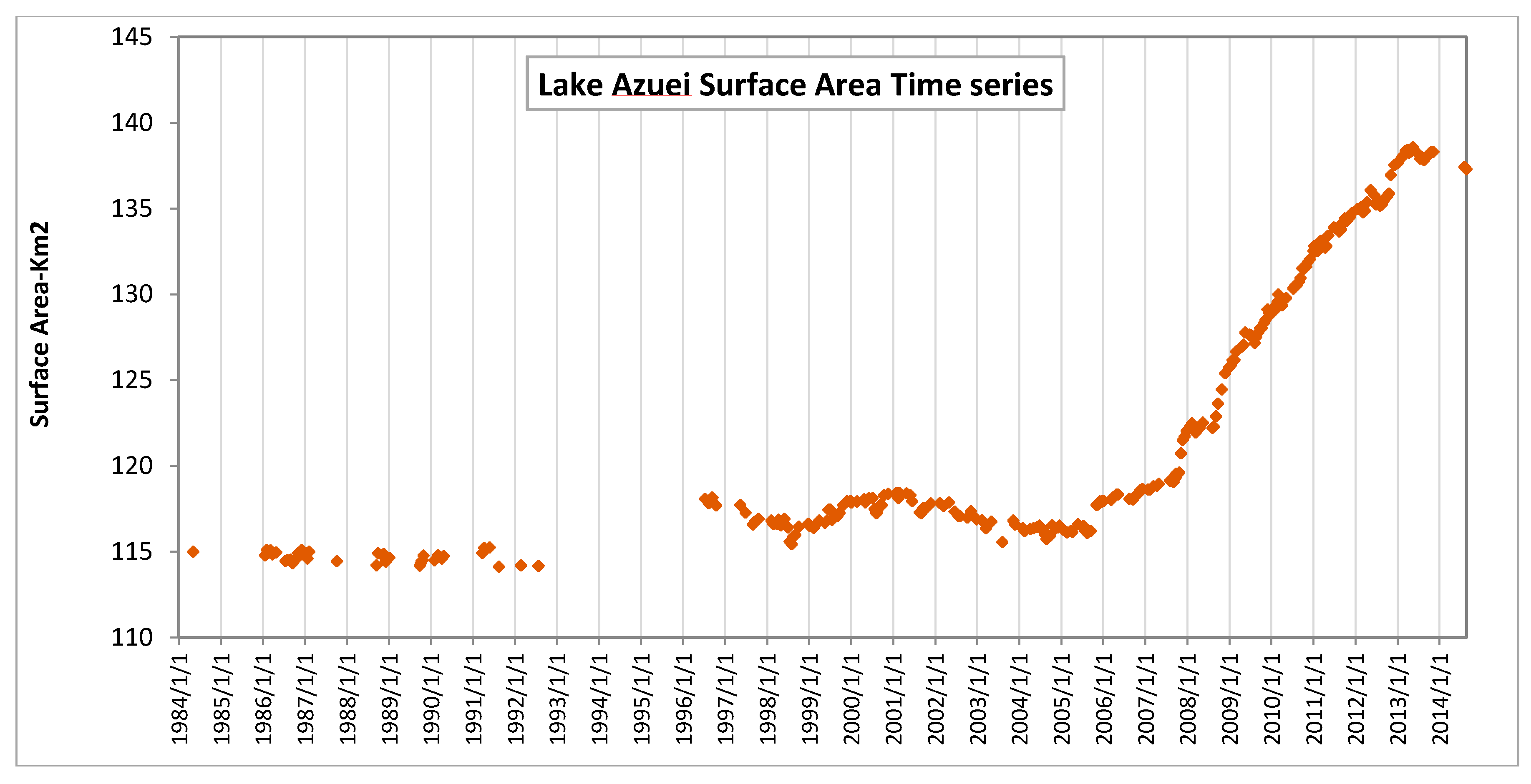
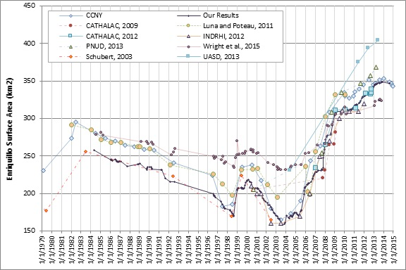
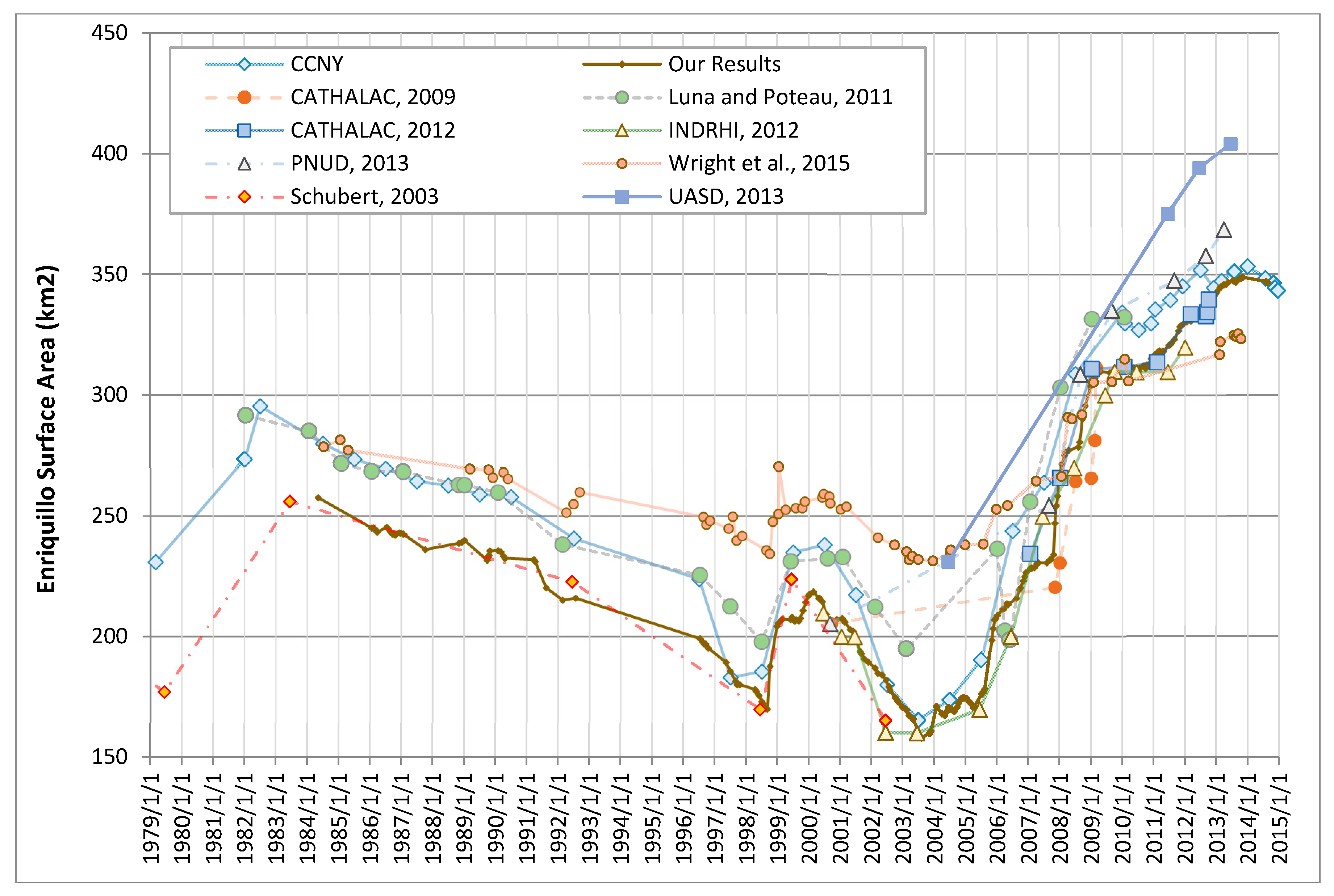
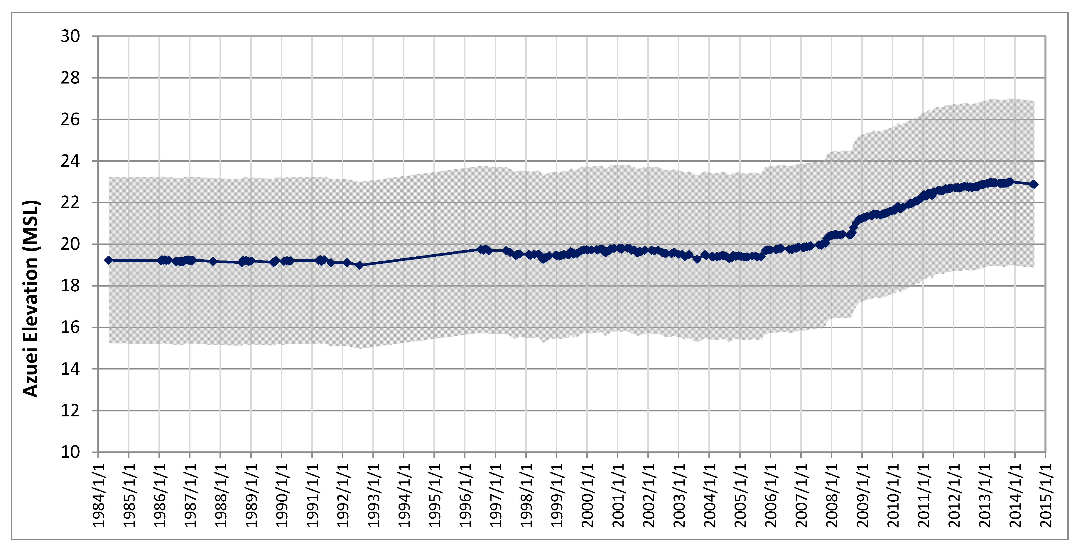
3.1. Lake Time Series
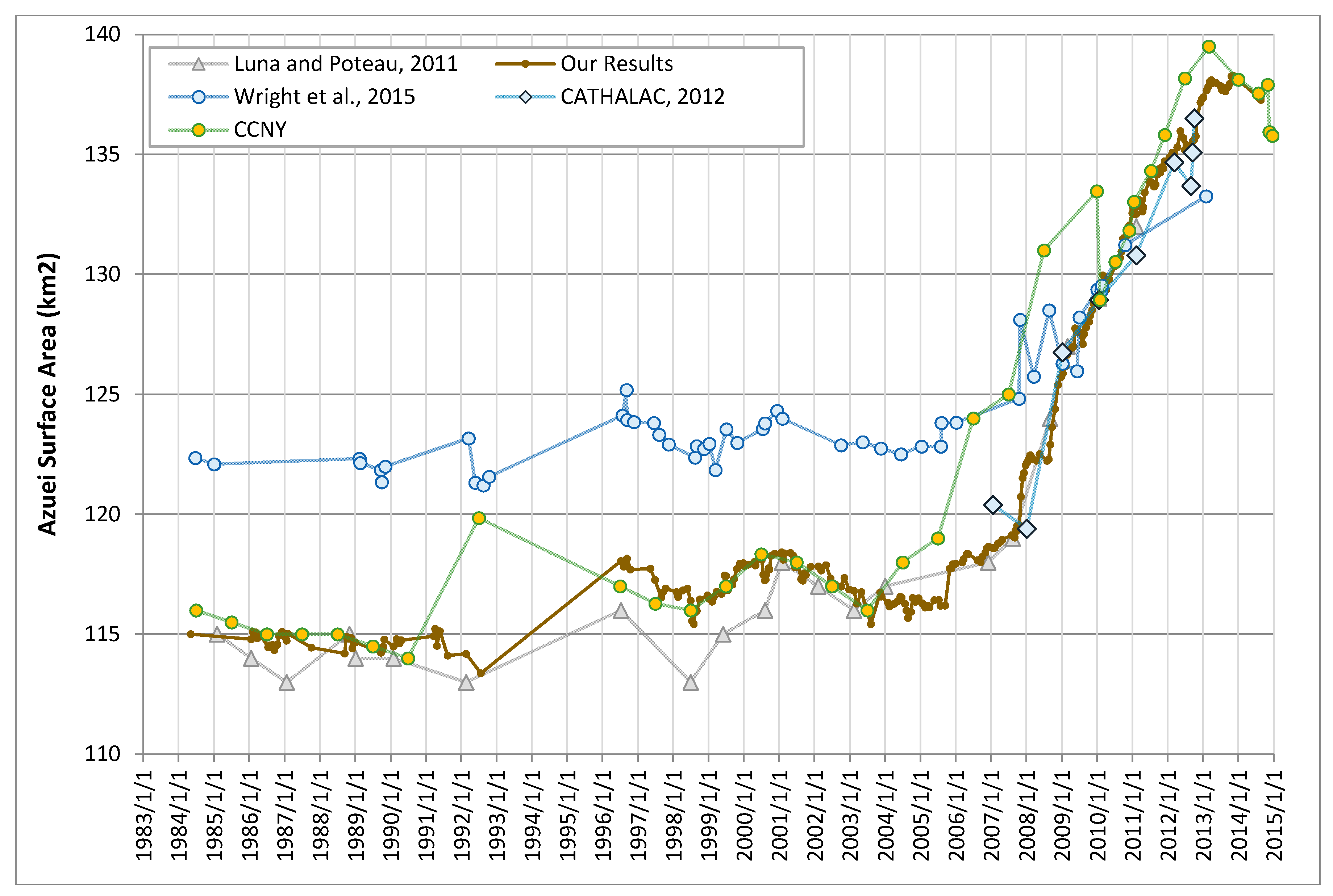
3.1.1. Previous Work
3.1.2. Time Series Development
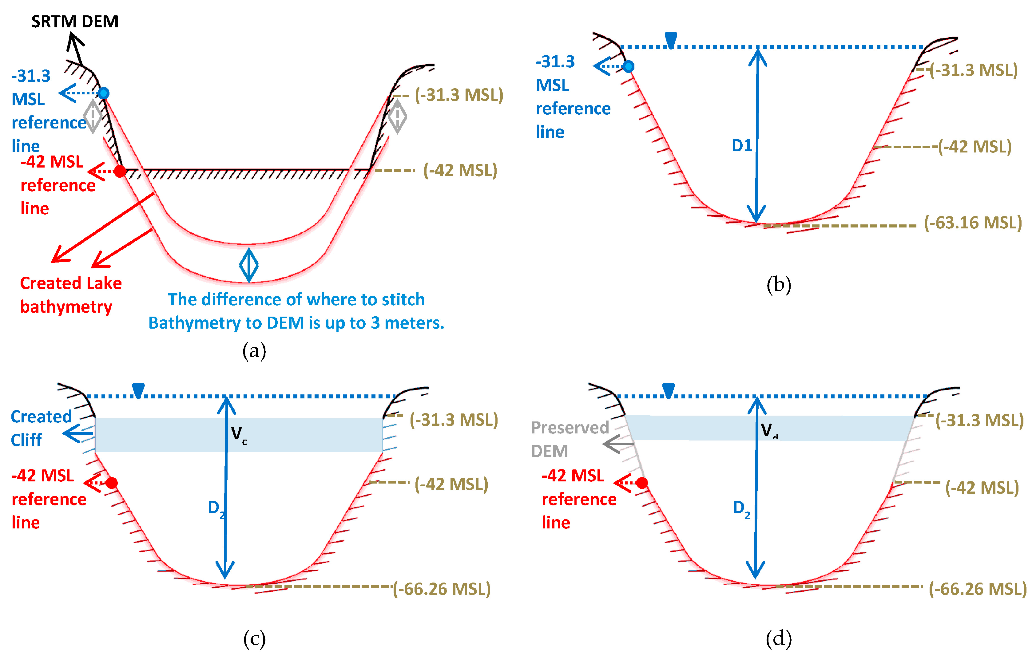
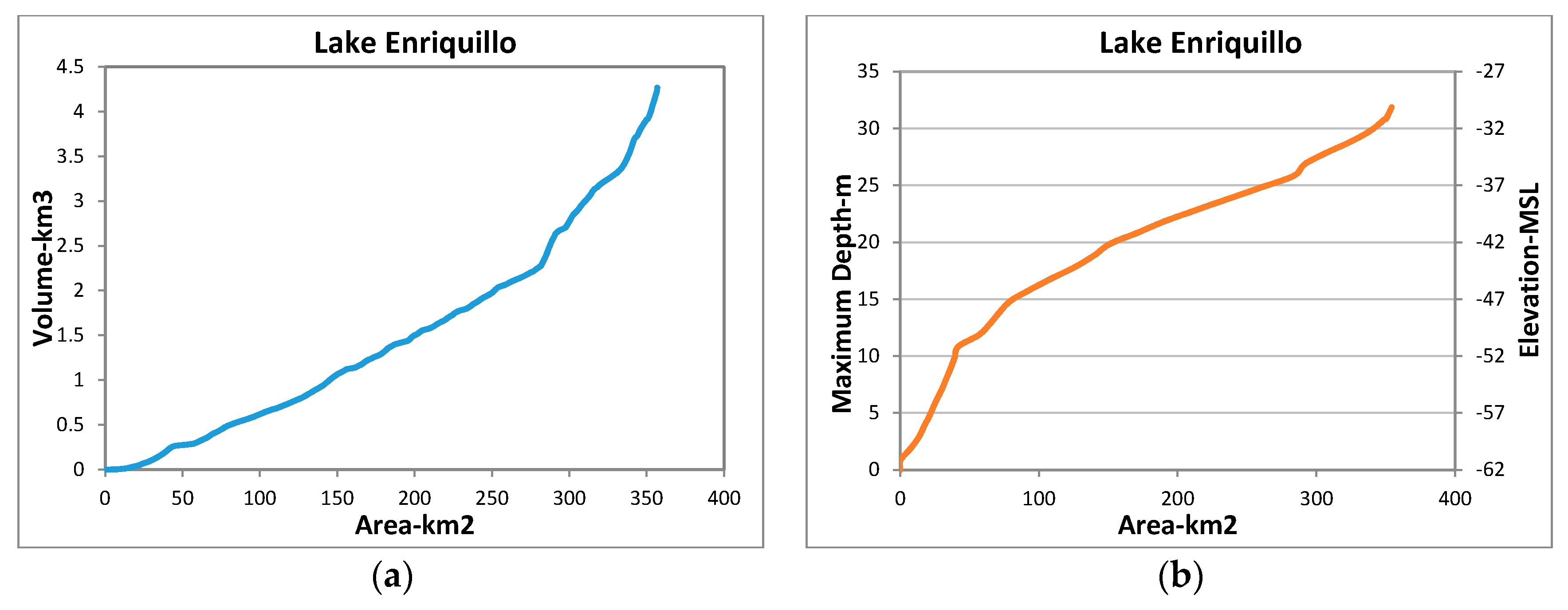
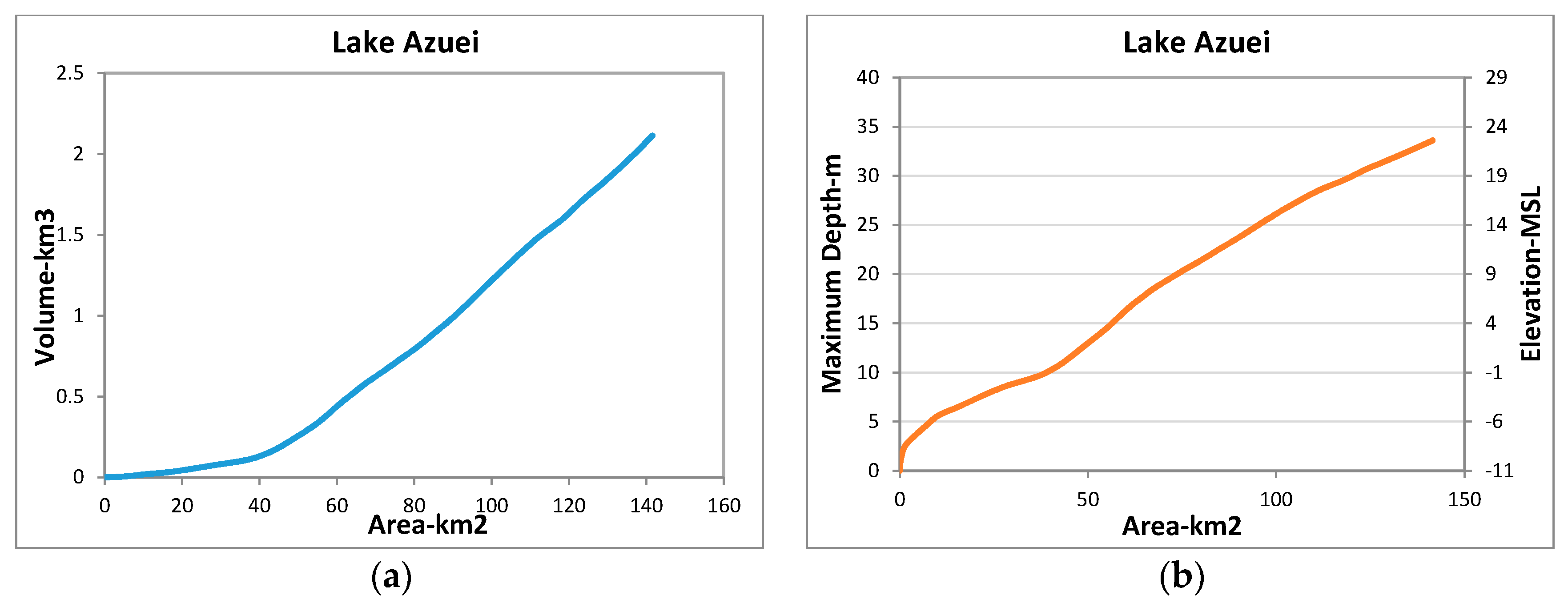
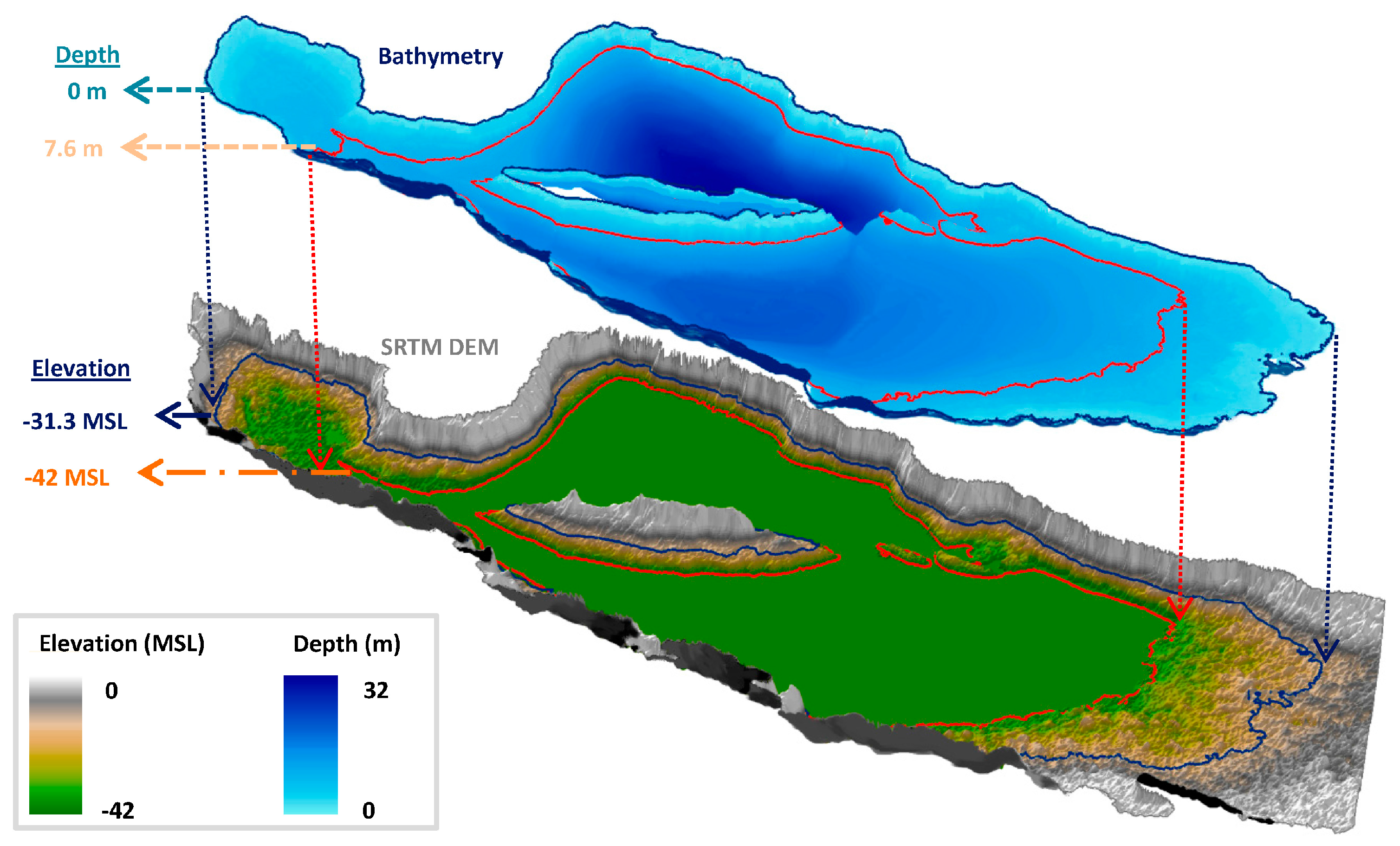
3.2. Bathymetric Data
3.3. Connecting DEM and Bathymetric Data
3.4. Rating Curves
4. Discussion
4.1. Lake Volumes
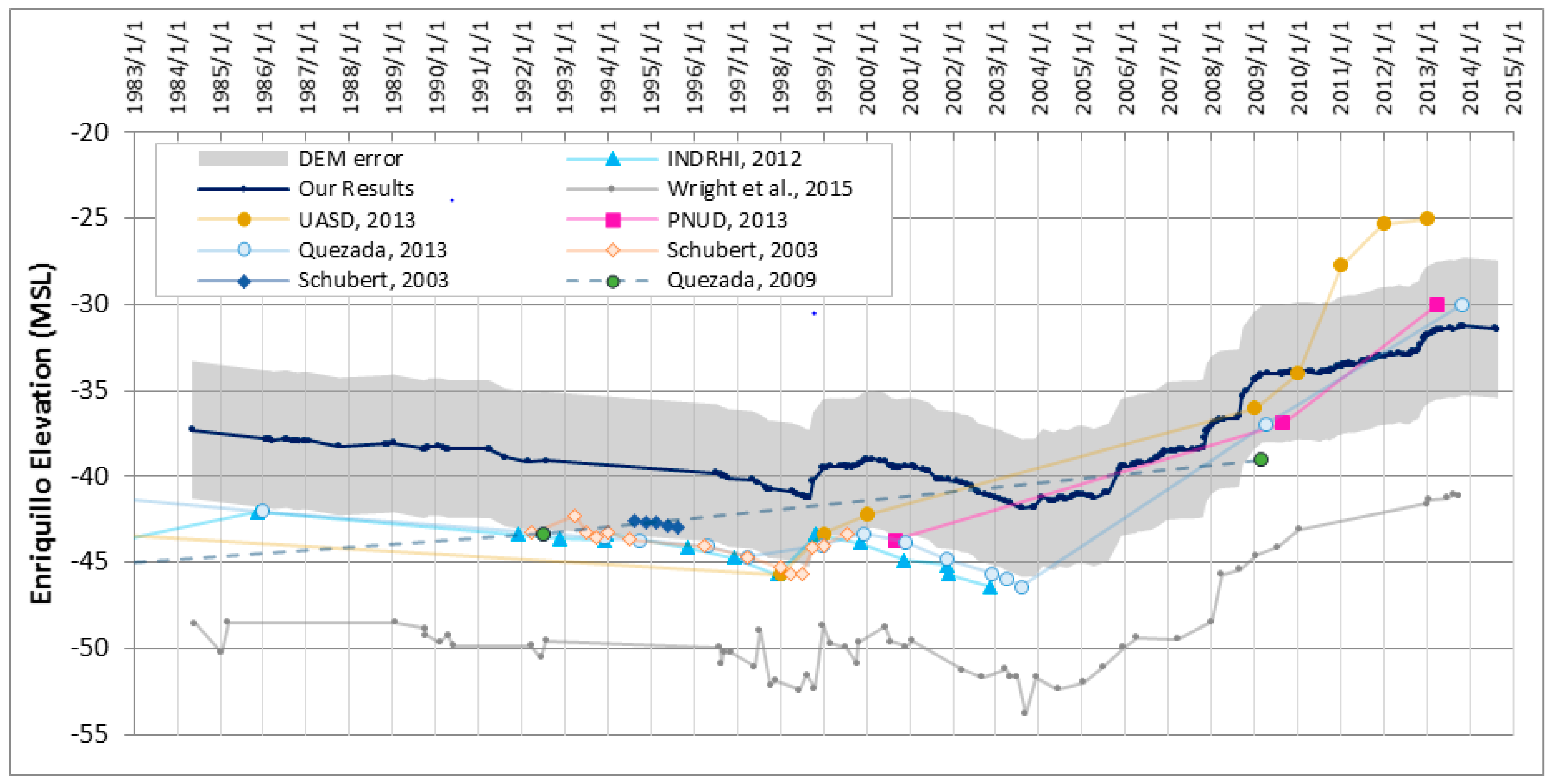
4.2. Lake Elevations
4.3. Future Lake Expansion
5. Conclusions
Acknowledgments
Author Contributions
Conflicts of Interest
References
- UN News Service. Haiti and Dominican Republic Partner to Save Border Lakes with UN’s Help. 2009. Available online: www.UN.org (accessed on 16 September 2009).
- The Guardian. Rapidly Rising Lake Levels Threaten Trade on Dominican-Haiti Border. 2012. Available online: www.TheGuardian.com (accessed on 31 August 2012).
- Archibold, R.C. Rising Tide Is a Mystery That Sinks Island Hopes. 2014. Available online: www.NYTimes.com (accessed on 11 January 2014).
- Arroyo, L. “El Agua se lo Llevó Todo”: El Misterio de Los Lagos Crecientes del Caribe. 2014. Available online: www.BBC.com (accessed on 16 January 2014).
- Europa Press. El Lago del Caribe que Crece de Forma Inexplicable. 2014. Available online: www.ABC.es (accessed on 16 January 2014).
- Vice News. The Lake That Burned Down a Forest (Lake Enriquillo, Dominican Republic). 2014. Available online: www.News.Vice.com (accessed on 27 July 2014).
- Kushner, J. The Relentless Rise of Two Caribbean Lakes Baffles Scientists. 2016. Available online: www.Nationalgeographic.com (accessed on 3 March 2016).
- Earth & Space Science News. Climate Change’s Pulse Is in Central America and the Caribbean. 2017. Available online: www.EOS.org (accessed on 27 April 2017).
- Perrissol, M.; Lescoulier, C. Etude Hydrologique et Hydrogéologique de la Montée des Eaux du Lac Azueï; Rapport de Mission, Version 2; Egis International: Haiti, 2011. [Google Scholar]
- Buck, D.; Brenner, M. Physical and chemical properties of hypersaline Lago Enriquillo, Dominican Republic. Int. Ver. Theor. Angew. Limnol. Verh. 2005, 29, 725–731. [Google Scholar]
- Méndez-tejeda, R.; Rosado, G.; Rivas, D.V.; Montilla, T.; Hernández, S.; Ortiz, A.; Santos, F. Climate variability and its effects on the increased level of Lake Enriquillo in the Dominican Republic, 2000–2013. Appl. Ecol. Environ. Sci. 2016, 4, 26–36. [Google Scholar]
- Logan, W.S.; Enfield, D.B.; Division, P.O.; Capdevila, A.S. Rising Water Levels at Lake Enriquillo, Dominican Republic: Advice on Potential Causes and Pathways forward. Report by the International Center for Integrated Water Resources Management (ICIWaRM) to the Instituto Nacional de Recursos Hidráulicos (INDRHI), Government of the Dominican Republic. 2012. Available online: https://s3.amazonaws.com/sitesusa/wp-content/uploads/sites/422/2015/12/Lake_Enriquillo_report_1-26-2012.pdf (accessed on 9 December 2015).
- Wright, V.D.; Hornbach, M.J.; Mchugh, C.; Mann, P. Factors contributing to the 2005-present, rapid rise in lake levels, Dominican Republic and Haiti (Hispaniola). Nat. Resour. 2015, 6, 465–481. [Google Scholar] [CrossRef]
- Luna, E.J.R.; Poteau, D. Water Level Fluctuations of Lake Enriquillo and Lake Saumatre in Response to Environmental Changes. Master’s Thesis, Cornell University, Ithaca, NY, USA, 2011. [Google Scholar]
- Fortun, J. Environmental Impacts on Lake Azuéï in Haiti due to Degradation of Its Watersheds; University of Puerto Rico: San Juan, Puerto Rico, 2011. [Google Scholar]
- Comarazamy, D.E.; González, J.E.; Moshary, F.; Piasecki, M. On the hydrometeorological changes of a tropical water basin in the Caribbean and its sensitivity to midterm changes in regional climate. J. Hydrometeorol. 2015, 16, 997–1013. [Google Scholar] [CrossRef]
- Araguás Araguás, L.; Mchelen, C.; Garcia, A.; Medina, J.; Febrillet, J. Estudio de la Dinamica del Lago Enriquillo: Segundo Informe de Avance; Project DOM/8/006; International Atomic Energy Agency: Vienna, Austria, 1995. [Google Scholar]
- Pichardo, F.D.G.; Conte, L.L.; Regio, G. Alternativas Productivas a Mediano y Largo Plazo Para las Familias Afectadas por la Crecida del Nivel del Lago Enriquillo; Study Report; OXFAM, FAO y Comisión Europea: Santo Domingo, Dominican Republic, 2012. [Google Scholar]
- Schubert, A. El Lago Enriquillo—Gran Patrimonio Natural y Cultural del Caribe, 2nd ed.; Secretaría de Medio Ambiente y Recursos Naturales Consorcio Ambiental Dominicano CAD: Jimaní, Dominican Republic, 2003. [Google Scholar]
- Piasecki, M.; Moknatian, M.; Moshary, F.; Cleto, J.; Leon, Y.; Gonzalez, J.; Comarazamy, D. Development of geospatial lake representations: Hispaniola’s Lake Azuei and Enriquillo. Caribb. J. Sci. 2015. accepted. [Google Scholar]
- González, R.; Brito, D.R.; González, J. Estudio Hidrogeológico de la Zona del Lago Enriquillo, Determinación de las Causas del Aumento de Nivel de sus Aguas e Intervenciones Requeridas para su Control; Informe No. 1 de Avance del Proyecto; INTEC/CCNY; 2010. [Google Scholar]
- Fritz, S.C.; Cumming, B.F.; Gasse, F.; Laird, K.R. Diatoms as indicators of hydrologic and climatic change in saline lakes. In The Diatoms: Applications for the Environmental and Earth Sciences; Stoermer, E.F., Smol, J.P., Eds.; Cambridge University Press: Cambridge, UK, 2001; Volume 102, pp. 186–208. [Google Scholar]
- Maiersperger, T.K.; Scaramuzza, P.L.; Leigh, L.; Shrestha, S.; Gallo, K.P.; Jenkerson, C.B.; Dwyer, J.L. Characterizing LEDAPS surface reflectance products by comparisons with AERONET, field spectrometer, and MODIS data. Remote Sens. Environ. 2013, 136, 1–13. [Google Scholar] [CrossRef]
- Chávez, P.S.J. Image-Based Atmospheric Corrections—Revisited and Improved. Photogramm. Eng. Remote Sens. 1996, 62, 1025–1036. [Google Scholar]
- Martinuzzi, S.; Gould, W.; González, O. Creating Cloud-Free Landsat ETM+ Data Sets in Tropical Landscapes: Cloud and Cloud-Shadow Removal; General Technical Report IITF-GTR-32; International Institute of Tropical Forestry: Ro Piedras, Puerto Rico, 2007. [Google Scholar]
- Jedlovec, G. Automated Detection of Clouds in Satellite Imagery. Advances in Geoscience and Remote Sensing, 2009. Available online: https://www.intechopen.com/books/advances-in-geoscience-and-remote-sensing/automated-detection-of-clouds-in-satellite-imagery (accessed on 22 May 2017).
- Irish, R.R. Landsat 7 automatic cloud cover assessment. AeroSense 2000, 4049, 348–355. [Google Scholar]
- Huang, C.; Thomas, N.; Goward, S.N.; Masek, J.G.; Zhu, Z.; Townshend, J.R.G.; Vogelmann, J.E. Automated masking of cloud and cloud shadow for forest change analysis using Landsat images. Int. J. Remote Sens. 2010, 31, 5449–5464. [Google Scholar] [CrossRef]
- Hughes, M.; Hayes, D. Automated detection of cloud and cloud shadow in single-date Landsat imagery using neural networks and spatial post-processing. Remote Sens. 2014, 6, 4907–4926. [Google Scholar] [CrossRef]
- Irish, R.R.; Barker, J.L.; Goward, S.N.; Arvidson, T. Characterization of the Landsat-7 ETM+ Automated Cloud-Cover Assessment (ACCA) Algorithm. Photogramm. Eng. Remote Sens. 2006, 72, 1179–1188. [Google Scholar] [CrossRef]
- Zhu, Z.; Wang, S.; Woodcock, C.E. Improvement and expansion of the Fmask algorithm: Cloud, cloud shadow, and snow detection for Landsats 4-7, 8, and Sentinel 2 images. Remote Sens. Environ. 2015, 159, 269–277. [Google Scholar] [CrossRef]
- Zhu, Z.; Woodcock, C.E. Object-based cloud and cloud shadow detection in Landsat imagery. Remote Sens. Environ. 2012, 118, 83–94. [Google Scholar] [CrossRef]
- Helmer, E.H.; Ruefenacht, B. Cloud-free satellite image mosaics with regression trees and histrogram matching. Photogramm. Eng. Remote Sens. 2005, 71, 1079–1089. [Google Scholar] [CrossRef]
- Wang, B.; Ono, A.; Muramatsu, K.; Fujiwara, N. Automated detection and removal of clouds and their shadows from Landsat TM images. IEICE Trans. Inf. Syst. 1999, 82, 453–460. [Google Scholar]
- Jin, S.; Homer, C.; Yang, L.; Xian, G.; Fry, J.; Danielson, P.; Townsend, P.A. Automated cloud and shadow detection and filling using two-date Landsat imagery in the USA. Int. J. Remote Sens. 2013, 34, 1540–1560. [Google Scholar] [CrossRef]
- Li, W.; Du, Z.; Ling, F.; Zhou, D.; Wang, H.; Gui, Y.; Sun, B.; Zhang, X. A comparison of land surface water mapping using the Normalized Difference Water Index from TM, ETM+ and ALI. Remote Sens. 2013, 5, 5530–5549. [Google Scholar] [CrossRef]
- Li, M.; Xu, L.; Tang, M. An extraction method for water body of remote sensing image based on oscillatory network. J. Multimed. 2011, 6, 252–260. [Google Scholar] [CrossRef]
- Xu, H. Modification of normalised difference water index (NDWI) to enhance open water features in remotely sensed imagery. Int. J. Remote Sens. 2006, 27, 3025–3033. [Google Scholar] [CrossRef]
- Jiang, H.; Feng, M.; Zhu, Y.; Lu, N.; Huang, J.; Xiao, T. An automated method for extracting rivers and lakes from Landsat Imagery. Remote Sens. 2014, 6, 5067–5089. [Google Scholar] [CrossRef]
- McFeeters, S.K. Using the normalized difference water index (NDWI) within a geographic information system to detect swimming pools for mosquito abatement: A practical approach. Remote Sens. 2013, 5, 3544–3561. [Google Scholar] [CrossRef]
- Wilson, E.H.; Sader, S.A. Detection of forest harvest type using multiple dates of Landsat TM imagery. Remote Sens. Environ. 2002, 80, 385–396. [Google Scholar] [CrossRef]
- Shen, L.; Li, C. Water body extraction from Landsat ETM+ imagery using adaboost algorithm. In Proceedings of the 18th International Conference on Geoinformatics, Beijing, China, 18–20 June 2010; pp. 3–6. [Google Scholar]
- Daniels, R.C. Using ArcMap to extract shorelines from Landsat TM & ETM+ data. In Proceedings of the Thirty-Second ESRI International Users Conference, San Diego, CA, USA, 12–16 July 2010; pp. 1–23. [Google Scholar]
- Feyisa, G.L.; Meilby, H.; Fensholt, R.; Proud, S.R. Automated Water Extraction Index: A new technique for surface water mapping using Landsat imagery. Remote Sens. Environ. 2014, 140, 23–35. [Google Scholar] [CrossRef]
- Ji, L.; Zhang, L.; Wylie, B. Analysis of dynamic thresholds for the Normalized Difference Water Index. Photogramm. Eng. Remote Sens. 2009, 75, 1307–1317. [Google Scholar] [CrossRef]
- Chen, J.; Zhu, X.; Vogelmann, J.E.; Gao, F.; Jin, S. A simple and effective method for filling gaps in Landsat ETM+ SLC-off images. Remote Sens. Environ. 2011, 115, 1053–1064. [Google Scholar] [CrossRef]
- Zhang, C.; Li, W.; Travis, D. Gaps-fill of SLC-off Landsat ETM+ satellite image using a geostatistical approach. Int. J. Remote Sens. 2007, 28, 5103–5122. [Google Scholar] [CrossRef]
- Afshari, S. sha17hab/Flood-Inundation-Mapping-and-Comparison-of-Two-Models: Flood-Inundation-Mapping-and-Comparison-of-Two-Models. Zenodo 2016. [Google Scholar] [CrossRef]
- Schubert, A. Lagos Enriquillo y Azuéi. Donde la Naturaleza Siempre Tiene Una Sorpresa; Editorial Académica Española, Ed.; LAP Lambert Academic Publishing GmbH & Co. KG: Saarbrücken, Germany, 2012. [Google Scholar]
- Quezada, A.C. El Ciclo Hidrologico del Lago Enriquillo y la Crecida Extrema del, 2009. Available online: http://www.acqweather.com/EL%20CICLO%20HIDROLOGICO%20DEL%20LAGO%20ENRIQUILLO.pdf (accessed on 16 April 2009).
- Quezada, A.C. La Oscilacion Natural del Lago Enriquillo (ONLE): Un Evento Hidrometeorológico que Responde a la Variabilidad Climática de la República Dominicana. Available online: http://www.acqweather.com/LA%20ONLE%20Final.pdf (accessed on 24 December 2013).
- Programa de Naciones Unidas para el Desarrollo (PNUD). Plan Estratégico de Recuperación y Transición al Desarrollo para la Zona del Lago Enriquillo; Editora Búho, Proyecto Frontera—UNDP: Santo Domingo, Dominican Republic, 2013. [Google Scholar]
- The Hispaniola Lakes Project. Available online: http://cuerg.ccny.cuny.edu/hispaniola (accessed on 30 December 2016).
- CATHALAC. Expansion of Haiti’s Lake Azuei. Available online: http://www.un-spider.org/news-and-events/news/cathalac-subsequent-analysis-lake-azuei-flooding (accessed on 2 October 2012).
- Buck, D.G. Limnology and Paleolimnology of Hypersaline Lago Enriquillo, Dominican Republic. Master’s Thesis, University of Florida, Gainesville, FL, USA, 2004. [Google Scholar]
- INTEC (Instituto Tecnológico de Santo Domingo). Científicos Completan el Mapa de Fondo de los Lagos Enriquillo y Azuéi. Available online: http://www.intec.edu.do/noticias-y-actividades/noticias/item/cientificos-completan-el-mapa-de-fondo-de-los-lagos-enriquillo-y-azuei (accessed on 12 September 2013).
- Rodriguez, E.; Morris, C.S.; Belz, J.E.; Chapin, E.C.; Martin, J.M.; Daffer, W.; Hensley, S. An Assessment of the SRTM Topographic Products; Technical Report JPL; Jet Propulsion Laboratory: Pasadena, CA, USA, 2005. [Google Scholar]


| Satellite | Sensor | Year | Number of Bands | Resolution (m) | Number of Available Images | Percentage of the Cloud-Free Scene | Data Gaps |
|---|---|---|---|---|---|---|---|
| Landsat-4 | TM | 1988–1992 | 7 | 30 | 9 | 0% | - |
| Landsat-5 | TM | 1984–2011 | 7 | 30 | 91 | 45% | - |
| Landsat-7 | ETM | 1999–2014 | 8 | 30 | 193 | 49% | 85% |
| WIs | Surface Area Error (%) | Overall Accuracy (%) | Kappa Coefficient | F-Overlapping (%) | Omission Error (%) | Commission Error (%) | Visual Inspection |
|---|---|---|---|---|---|---|---|
| NDWI | −0.68 | 99.997 | 0.99 | 99.32 | 0.68 | 0.00 | Good |
| MNDWI | +4.20 | 99.97 | 0.96 | 92.68 | 5.82 | 1.69 | Detects wet land as water |
| NDMI | +209.94 | 99.09 | 0.46 | 29.78 | 5.93 | 69.65 | Not good |
| WRI | +1.38 | 99.99 | 0.99 | 98.28 | 0.18 | 1.55 | Detects wet land as water |
| NDVI | −1.01 | 99.996 | 0.99 | 98.99 | 1.01 | 0.00 | Unable to detect shallow water |
| AWEInsh | +5.23 | 99.68 | 0.93 | 83.57 | 4.62 | 1.43 | Detects wet land as water |
| AWEIsh | +1.11 | 99.99 | 0.99 | 98.85 | 1.18 | 1.02 | Good |
| WIs | Surface Area Error (%) | Overall Accuracy (%) | Kappa Coefficient | F-Overlapping (%) | Omission Error (%) | Commission Error (%) | Visual Inspection |
|---|---|---|---|---|---|---|---|
| NDWI | −0.87 | 99.72 | 0.99 | 98.79 | 1.04 | 0.32 | Good |
| MNDWI | −4.48 | 98.85 | 0.97 | 95.09 | 4.70 | 1.42 | Unable to detect hill-shade on the shoreline |
| NDMI | +32.29 | 90.17 | 0.75 | 69.41 | 11.36 | 28.06 | Not good |
| WRI | −1.59 | 99.63 | 0.99 | 98.41 | 1.59 | 0.48 | Good |
| NDVI | −29.69 | 93.04 | 0.78 | 70.31 | 29.69 | 8.33 | Not good |
| AWEInsh | +2.41 | 99.37 | 0.97 | 87.64 | 3.22 | 1.36 | Unable to detect hill-shade on the shoreline |
| AWEIsh | −1.81 | 99.51 | 0.98 | 98.03 | 1.79 | 0.68 | Good |
| Date of Gathering GPS Data | Landsat Image Date | Image Quality | Lake | GPS Points Position | Maximum Distance (m) | Minimum Distance (m) | Mean Distance (m) | Standard Deviation |
|---|---|---|---|---|---|---|---|---|
| 25–26 March 2013 | 27 March 2013 | -Clear scene -Existence of gaps | Enriquillo | GPS points fall inside the delineated lake extent | 94.57 | 0.18 | 41.07 | 32.75 |
| GPS points are outside the delineated lake extent | 17.05 | 0.17 | 3.67 | 2.42 | ||||
| 19–24 June 2013 | 1 July 2013 | Existence of: -Gaps -Cloud -Cloud shadow | Azuei | GPS points fall inside the delineated lake extent | 89.61 | 0.03 | 35.25 | 21.51 |
| GPS points are outside the delineated lake extent | 36.58 | 0.03 | 8.38 | 6.33 |
| Lake | Date | Conditional Kappa for Water Body | F-Overlapping (%) | Overall Accuracy (%) | Surface Area (km2) | Absolute Error (km2) | Relative Error (%) |
|---|---|---|---|---|---|---|---|
| Enriquillo | 22 February 2001 | 0.989 | 98.72 | 99.76% | 206.036 | 0.53 | 0.26 |
| 19 September 2007 | 0.992 | 98.31 | 99.64% | 231.977 | 0.71 | 0.31 | |
| 21 August 2014 | 0.992 | 98.97 | 99.68% | 346.694 | 0.30 | 0.09 | |
| Azuei | 22 February 2001 | 0.995 | 98.59 | 99.67% | 118.368 | 0.56 | 0.47 |
| 19 September 2007 | 0.993 | 98.46 | 99.63% | 119.296 | 0.20 | 0.17 | |
| 21 August 2014 | 0.980 | 98.08 | 99.47% | 137.277 | 1.08 | 0.79 |
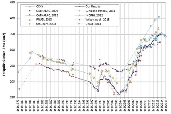
| Source | Timespan | Number of Data Points | Range of Values km2 | Data Used |
|---|---|---|---|---|
| INDRHI [12,17] | 2000–2012 | 14 * | 160–320 km2 * | Landsat Imagery |
| CATHALAC, 2009 [9,18,50,51] | 2000–2009 | 7 | 205–312 km2 | Landsat/MODIS |
| CATHALAC, 2012 [51] | 2007–2012 | 9 | 234–340 km2 | - |
| PNUD [52] | 2000–2013 | 7 | 205–369 km2 | - |
| UASD [52] | 2004–2013 | 4 | 231–404 km2 | - |
| CCNY [53] | 1979–2015 | 50 | 165–353 km2 | Landsat Imagery |
| Schubert, 2003 [19] | 1969–2002 | 7 | 165–269 km2 * | - |
| Luna and Poteau, 2011 [14] | 1982–2010 | 24 | 195–332 km2 | Landsat Imagery |
| Wright et al., 2015 [13] | 1984–2013 | 60 * | 231–325 km2 * | Landsat Imagery |
| Mendez et al., 2016 [11] | 1996–2013 | 9 | 22–46 km2 | - |
| Source | Timespan | Number of Data Points | Range of Values km2 | Data Used |
|---|---|---|---|---|
| CATHALAC, 2012 [54] | 2007–2012 | 9 | 119–137 km2 | - |
| CCNY [53] | 1979–2015 | 47 | 111–140 km2 | Landsat Imagery |
| Luna and Poteau, 2011 [14,49] | 1985–2011 | 21 | 113–132 km2 | Landsat Imagery |
| Wright et al., 2015 [13] | 1984–2013 | 49 * | 121–133 km2 * | Landsat Imagery |
| Source | Timespan | Number of Data Points | Range of Values (m) |
|---|---|---|---|
| UASD [11,52] | 1961–2011 | 11 | −45.7 to −27.7 |
| Quezada, 2013 [51] | 1893–2009 | 31 | −46.42 to +0.63 |
| Quezada, 2009 [18,50,51] | 1892–2009 | 14 | −45.7 to +0.63 |
| Schubert, 2003 [19] | 1992–1999 | 14 | −45.6 to −42.2 * |
| Schubert, 2003 [19] | 1994–1995 | 5 | −42.92 to −42.54 * |
| INDRHI [10,49] | 1949–2002 | 27 | −46.4 to −30.02 |
| PNUD [52] | 2000–2012 | 3 | −43.7 to −30 |
| Wright et al., 2015 [13] | 1984–2013 | 57 | −53.8 to −41.1 * |
© 2017 by the authors. Licensee MDPI, Basel, Switzerland. This article is an open access article distributed under the terms and conditions of the Creative Commons Attribution (CC BY) license (http://creativecommons.org/licenses/by/4.0/).
Share and Cite
Moknatian, M.; Piasecki, M.; Gonzalez, J. Development of Geospatial and Temporal Characteristics for Hispaniola’s Lake Azuei and Enriquillo Using Landsat Imagery. Remote Sens. 2017, 9, 510. https://doi.org/10.3390/rs9060510
Moknatian M, Piasecki M, Gonzalez J. Development of Geospatial and Temporal Characteristics for Hispaniola’s Lake Azuei and Enriquillo Using Landsat Imagery. Remote Sensing. 2017; 9(6):510. https://doi.org/10.3390/rs9060510
Chicago/Turabian StyleMoknatian, Mahrokh, Michael Piasecki, and Jorge Gonzalez. 2017. "Development of Geospatial and Temporal Characteristics for Hispaniola’s Lake Azuei and Enriquillo Using Landsat Imagery" Remote Sensing 9, no. 6: 510. https://doi.org/10.3390/rs9060510