
Trends in Greenness and Snow Cover in Alaska’s Arctic National Parks, 2000–2016


Arctic Inventory and Monitoring Network, National Park Service, Fairbanks, AK 99709, USA
Remote Sens. 2017, 9(6), 514; https://doi.org/10.3390/rs9060514
Submission received: 11 March 2017
/
Revised: 11 May 2017
/
Accepted: 16 May 2017
/
Published: 23 May 2017
(This article belongs to the Special Issue Remote Sensing of Arctic Tundra)
Abstract
:In cold-limited arctic environments, the duration and timing of the snow cover and the vegetation green season have major ecological implications. I monitored the phenology of snow cover and greenness using MODIS Terra satellite data for the years 2000 to 2016 in the 5 National Parks of northern Alaska, USA. Mann-Kendall trend tests showed that the end of the continuous snow season and midpoint of spring green-up became significantly earlier in parts of the study area over the 16-year period. Using the observed relationship between thaw degree-days at Kotzebue, Alaska and dates of snow-off and half green-up in nearby lowland tundra for the 16 years of MODIS data, I reconstructed the dates of snow-off and half green-up from long-term Kotzebue weather records back to 1937. The average snow-off and green-up dates probably became earlier by about 6 days over this 80-year time interval. Remote sensing of fall vegetation senescence and establishment of the snow cover were less reliable than the spring events due to cloudiness and low sun angles. The annual maximum normalized difference vegetation index (NDVI) generally did not increase significantly from 2001 to 2016, except in places where vegetation was recovering from forest fires.

1. Introduction
The climate of the Arctic has been warming since about 1980 [1] and the timing of spring snow loss has become significantly earlier over the same period [2]. Greenness of the Arctic land surface, based on normalized difference vegetation index (NDVI) calculated from the Global Inventory Modeling and Mapping Studies (GIMMS) dataset (8-km resolution) has increased over much of the Arctic since the 1980s, though there are some exceptions and a recent overall decline [3,4,5,6]. In view of the fundamental importance of snow cover and terrestrial plant productivity to ecosystems in the National Parks of northern Alaska, the National Park Service is monitoring vegetation and snow phenology as a part of its long-term monitoring program [7,8,9,10]. The MODIS (Moderate Resolution Imaging Spectroradiometer, [11]) Terra satellite has been providing spectral information with 250 m resolution on a daily basis since the year 2000. These images can be used to determine greenness and snow cover, and allow us to study the magnitude and timing of changes in the seasons at finer spatial and temporal resolution than was possible previously.
The purpose of this study is to explore the following questions for the National Parks of northern Alaska: (1) Are the disappearance of snow and the green-up occurring earlier in the spring? (2) Is peak greenness becoming more intense? (3) Are fall senescence and the establishment of snow cover occurring later? My results show that spring snow-off and green-up have indeed become earlier since the year 2000, continuing the long-term trend. However, peak greenness changed little; it increased significantly only where vegetation was recovering from forest wildfires (but not tundra fires) and colonizing newly drained lakebeds. Trends in the fall phenology events (vegetation senescence and establishment of the snow cover) remain poorly quantified due to cloudiness and the low sun angles of the study area during that time of year.
2. Materials and Methods
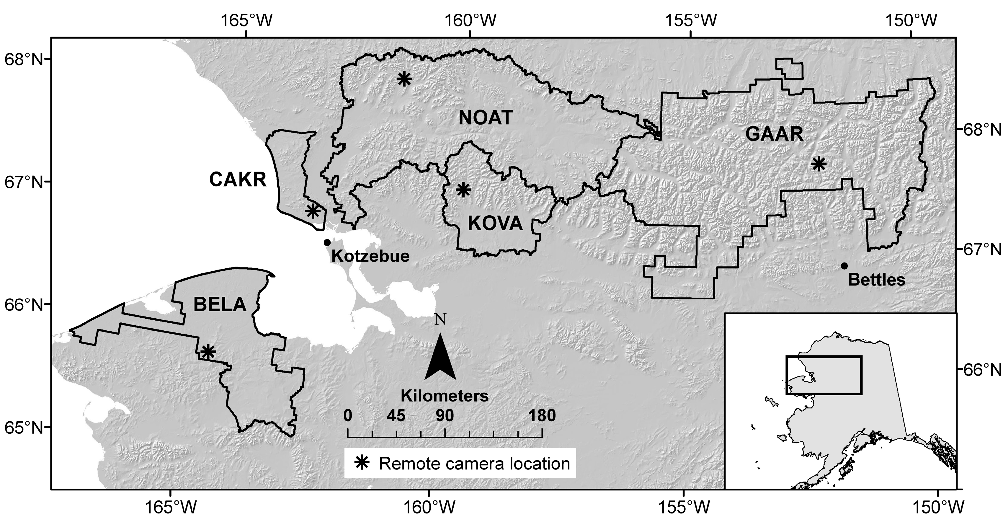
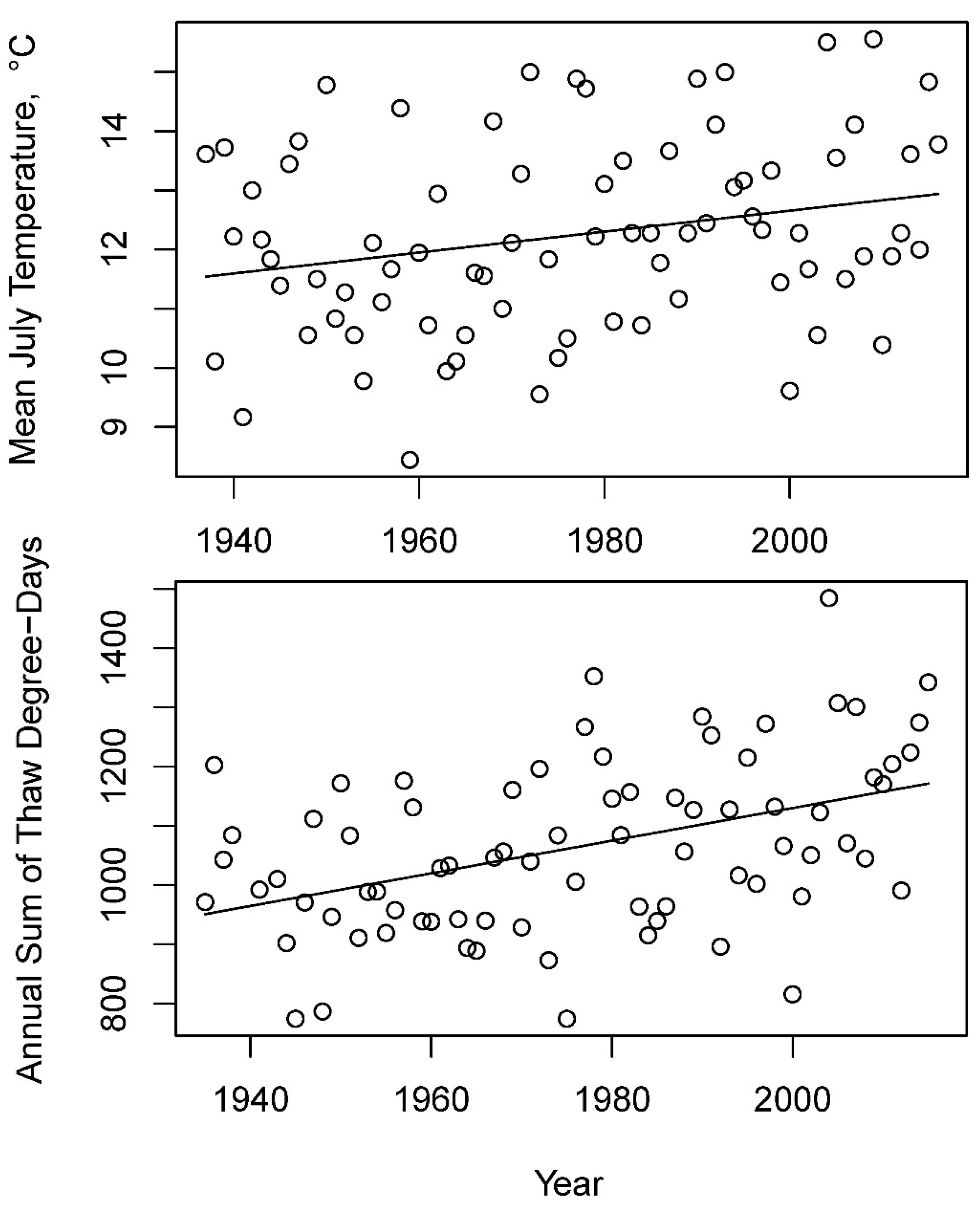
The study area is the five National Park Service (NPS) units in northern Alaska (Figure 1). These parks cover approximately 82,000 km2, including lowlands near sea level and rugged mountainous terrain with elevations that reach over 2000 m above sea level. The climate is arctic and subarctic, with mean annual air temperatures ranging from about −5 °C at low elevations in the south and west to about −10 °C in the northern mountains. Mean January temperatures range from about −18 °C in the maritime west and at mid-elevations in the southern mountains, to about −25 °C in the valleys of Noatak National Preserve (NOAT) and Gates of the Arctic National Park and Preserve (GAAR). July temperatures range from about 15 °C at low elevations in southern inland locations, to about 10 °C near the coast and 5 °C in the highest mountains (temperatures are modeled 1971–2000 means by [12]). Long-term National Weather Service records from Kotzebue, Alaska (on the coast in the western part of the study area, Figure 1) show a gradual increase in the annual sum of thaw degree-days (a general index of growing season warmth [13]) and mean July temperatures since consistent records began in the late 1930s (Figure 2).
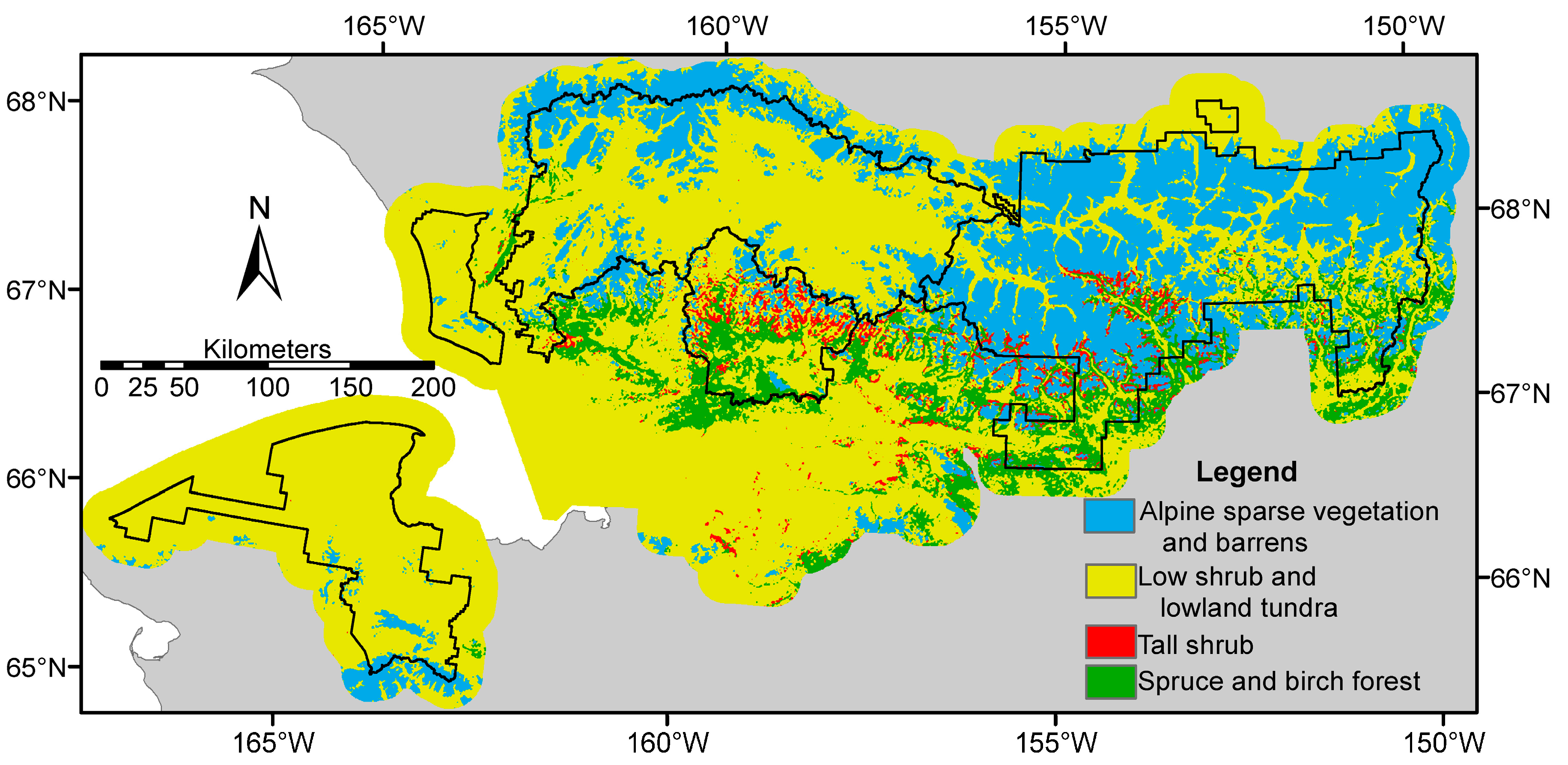
Most of the study area is arctic tundra or alpine barrens, with boreal forests of spruce (Picea mariana and P. glauca spp.) and birch (Betula neoalaskana) present at low elevations in southern inland locations (Figure 3). While the satellite data on which this study is based are available for all of Alaska, I chose to limit the geographic coverage of this study to these NPS lands, where I have detailed auxiliary data and extensive on-the-ground experience to aid in interpretation of the results. The study area encompasses about one-fourth of all NPS-administered lands in the United States.
The MODIS Terra Snow Cover Daily L3 Global 500 m Grid data (MOD10A1 collection 5; [16]) from the National Snow and Ice Data center (NSIDC) [17] were used to determine the snow season. The MODIS Terra satellite gathers multispectral data daily at 10:30 am local solar time. In cloud-free pixels, snow cover (snow present or absent), snow albedo (the percentage of solar radiation reflected), and fractional snow cover (estimated snow cover in percent) are mapped by the NSIDC using a snow mapping algorithm based on the Normalized Difference Snow Index (NDSI) and other criteria [16,18].
Determination of the start and end of the snow season is complicated by clouds and by the fact that snow cover in a season may be interrupted by snow-free periods. Additional processing of the daily NSIDC snow product, to interpolate across cloudy periods and detect the start and end of snow cover periods of different lengths, was performed by the Geographic Information Network of Alaska (GINA) at the University of Alaska, Fairbanks [19]. The GINA snow metrics algorithm locates the very first and last snow days in the snow year, along with the start and end of the longest of the continuous snow periods (defined as periods of continuous snow cover more than 2 weeks long with 2 or fewer days of no-snow) [20]. At the time of this research, data were available to determine snow-on dates from the fall of 2000 through the fall of 2015 and snow-off dates from the spring of 2001 through the spring of 2016 [21].
Vegetation greenness was studied using 7-day NDVI composites with 250 m resolution from the MODIS Terra satellite (collection 5), created as a part of the eMODIS project [22,23]. The eMODIS data were downloaded from the US Geological Survey [24]. The following growing-season metrics were computed by GINA from the eMODIS composites: the date of onset of green season, NDVI value at onset of greenness, maximum NDVI, date of end of green season, and NDVI value at the end of the green season. They used a weighted, windowed, least-squares linear regression algorithm to smooth the time-series data and remove local minima. Smoothed data points were obtained from linear regressions in a moving window, with local maxima receiving greater weight (1.5) than points on slopes (0.5) or local minima (0.005) [25]. The start and end of the green season were then identified by the delayed moving average method [26,27]. For each pixel in each year, a backward moving average was computed across the winter-spring transition. This backward average is dominated by winter values at the time of the start of green-up. The date when the smoothed NDVI curve crossed the backward-average curve as NDVI began its upward trend was recorded as the start of the growing season. Similarly, a forward moving average was computed in each year and each pixel for the fall, and the date when the decreasing NDVI curve crossed the forward-average curve was recorded as the end of the green season. At the time of this research, both the eMODIS product and GINA derivatives were available for the growing seasons from 2000 through 2015 [28].
Degradation of the MODIS Terra sensor may potentially influence NDVI time series [29]. The rate of NDVI change due to sensor degradation was estimated to be −0.001 to −0.004 NDVI units yr-1 during 2002–2010 [29]. The potential bias introduced by this sensor degradation is discussed in the Results and Discussion section below.
I computed two additional metrics from the NDVI data: the dates of the midpoint of spring green-up and midpoint of fall senescence. These halfway points are interesting ecologically because they represent the time of greatest rate of change; they are also easily compared to our ground verification data (see below), where we fit a sigmoid curve to the annual greenness time series and locate similar midpoints. Using the “raster” (version 2.3-40) and “rgdal” (version 0.9-2) packages in R (version 3.0.1) statistical software [30,31,32], I computed the median NDVI value across the 16 years of data for the onset of the green season, the median maximum NDVI, and the median NDVI at the end of green season from the GINA metrics. I then computed for each pixel the NDVI value halfway between median at onset of greenness and the median maximum value (the spring midpoint NDVI), and also between the median maximum and the median end of green season value (the fall midpoint NDVI). I created an annual NDVI curve for each pixel in each year by linear interpolation between the weekly eMODIS composite values (after removal of local minima that represent cloud contamination). I then located the spring and fall median midpoint NDVI values on the annual interpolated curve to estimate the dates of the spring and fall NDVI midpoint (half green-up and half senescence) in each year. Additional details and the R scripts are provided in [33,34].
I summarized the various growing-season metrics by geographic zones derived from ecological subsections [35,36,37,38,39]. Ecological subsections are areas with a consistent pattern of landforms, vegetation and climate. I aggregated adjacent similar ecological subsections to obtain 2 to 4 ecological zones (or “ecozones” below) per NPS unit (Figure 4).
Low sun angles create problems for sensing some phenology events at high latitudes. The solar zenith angle at summer solstice at the time of MODIS Terra’s pass (10:30 am local solar time) ranges in the Arctic Inventory and Monitoring Network (ARCN) from about 44° to 48° (42° to 46° above the horizontal), depending on the latitude. The solar zenith angle is more than 80° (i.e., the sun is less than 10° above the horizontal) at the time of the MODIS Terra satellite’s pass from late October through late February, and the solar zenith angle is more than 70° (the sun is less than 20° above the horizontal) from late September through late March (see the Supplementary Materials, Table S1). When the solar zenith angle is 70°, 39% of the land area in ARCN is in terrain shadow, and when the solar zenith angle is 80°, 57% of ARCN is in terrain shadow (see the Supplementary Materials, Figure S1). Thus, spring phenology events (snow-off and green-up), which occur in April, May, and June, are relatively unaffected by illumination issues. Fall phenology events (vegetation senescence and establishment of the snow cover) occur in August, September, October, and locally even in November (in years of late snow cover establishment). Thus, some fall events may occur after the landscape has gone into terrain shadow for the winter. This issue is compounded by cloudiness: 2 to 5 years of missing data out of 16 years due to clouds was typical for all ecological zones and compositing periods in September and October. Thus a fall event may be missed if it occurs after shadows arrive in October, or if cloudiness obscures it until those shadows arrive.
I used the modeled mean monthly temperatures by the PRISM Climate Group [12] (771 m resolution, for 1971–2000) to study the link between monthly average temperatures and median spring snow-off dates. I linearly interpolated between the monthly mean temperatures to estimate daily mean temperatures for each pixel. I located the median dates for the end of continuous snow season on the temperature curve of each pixel and determined the sum of thaw degree-days for the snow-off date.
I used long-term weather records to extrapolate the snow-off and half green-up dates determined from MODIS (2000–2016) into the past (prior to the year 2000) as follows. The Kotzebue National Weather Service station has continuous data from the present back to 1951 and discontinuous data to 1937 [14]. Kotzebue is the only long-term weather station near the study area that represents windy tundra areas with thin snowpacks. The data showed that few to no thaw degree-days were required to melt these thin tundra snowpacks; hence data on winter snow depth (which were not available) are not essential to understand snow-off and green-up in these areas. Using monthly mean temperatures, I computed the ordinal date (0 to 365) when the mean daily temperature exceeded 0 °C each year and correlated this date with the observed median end of the continuous snow season (CSS) from the MODIS data in nearby ecological zones. I used this regression relation (which had a slope very close to 1) to reconstruct the end of CSS back to the beginning of records at Kotzebue. I also computed (from the monthly means) the ordinal date when various thaw degree-day sums were exceeded at Kotzebue (60, 80, 100, … 220, 240 °C-days). I computed the median half green-up date for each year in each ecological zone using the MODIS data (2001–2016), and the correlation between these dates and the thaw degree-day sums at Kotzebue. I chose the degree-day sum and zone that produced the best correlation between the date when this sum was reached and the half green-up date in the zone, and used this regression and the historic temperature records at Kotzebue to reconstruct spring green-up dates at Kotzebue back to 1937. Thaw degree-days have been used successfully to predict spring phenology events in the Arctic [40], and tests of other base temperatures, both above and below 0 °C have shown that 0 °C is probably the best compromise value for base temperature [13].
Ground verification of satellite phenology observations was obtained from automated cameras at five NPS climate monitoring stations (Figure 1, [10]). The cameras were installed in 2013, but most of the data are from 2015–2016 when power-supply issues were solved and all were operational. At each location an analysis window was defined (see Supplementary Materials Figure S2) and analyzed quantitatively for greenness and snow cover as described in [10]. Greenness was computed from the mean red (R), green (G), and blue (B) digital counts in the analysis window using the “Percent green” criterion: g% = 100 × G/(R + G + B) [41,42]. A sigmoid curve was fitted to greenness to identify the midpoint day of the transition from low to high greenness in the spring and high to low greenness in the fall [10]. At locations where strong red colors were observed in the fall, there was no sigmoid transition, but instead a distinct fall minimum greenness coinciding with maximum redness that was located and its date recorded [10]. The start of the continuous snow season (more than 2 weeks of continuous snow) was also recorded for the fall, as was the date when the winter snowpack covered less than 50% of the analysis window in the spring [10]. These phenology metrics were compared with the satellite-derived dates for the same years by simply extracting the MODIS-derived pixel values for analogous metrics at the camera locations. Only approximate correspondence between the two measurements was expected, because of the very different areas sampled by the two methods: a small oblique window close to the ground by the camera (Figure S2) versus a 250 m (greenness) or 500 m (snow) pixel by MODIS. Also, the ground and satellite sensors provide different wavelengths to derive the phenology metrics.
Temporal trends across the years of available data for the metrics described above (e.g., spring midpoint NDVI date) were analyzed on a pixel-by-pixel basis using the Mann-Kendall test with Theil-Sen’s slope estimator. The Mann-Kendall test is a non-parametric test for the significance of a monotonic trend. It is based on the direction of change over time between all pairs of observations and does not assume normality or linearity of trend [43]. The Theil-Sen slope is a related non-parametric slope estimate: the median of slopes between all pairs of observations separated by time [44]. I implemented the Mann-Kendall test and Theil-Sen slope in the “rkt” package in R [45] using the “raster” package [31]. Additional details and the R scripts are available in [34].
To investigate the effect of fires on trends in maximum NDVI, I examined the results of the Mann-Kendall test within the mapped perimeters of fires from different years. Fire perimeters were obtained from the Alaska Interagency Coordination Center [46].
3. Results and Discussion
3.1. End of the Continuous Snow Season
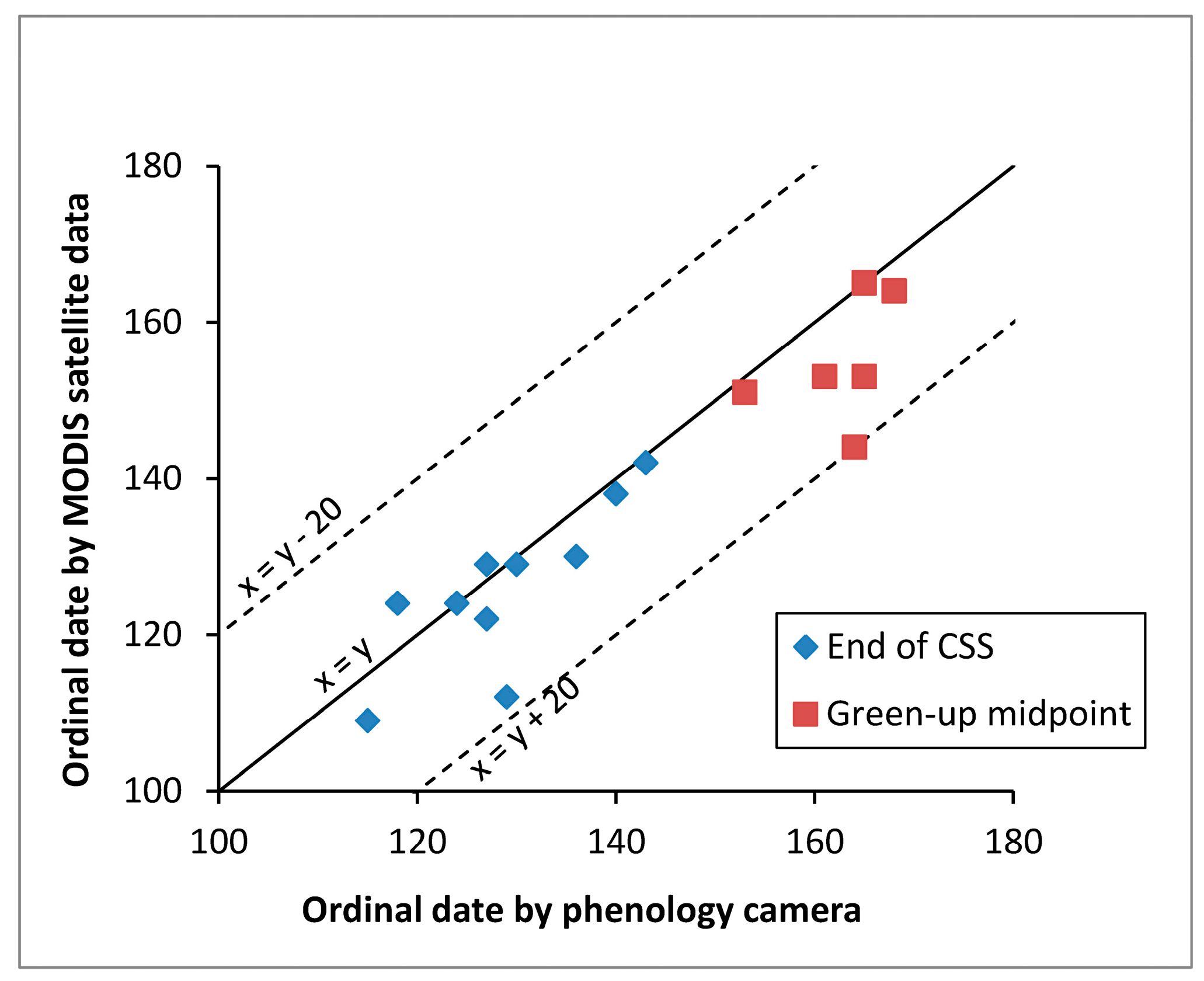
The median end of the continuous snow season (CSS) occurred in May across most of the study area (Figure S3). Snow-off prior to May 1 within the study area occurred in some windy tundra locations, while June snow-off dates occurred mainly in high mountain areas. Comparison of MODIS end of CSS with the snow-off dates registered by our phenology cameras showed good agreement (Figure 5). The median difference (MODIS date minus camera date) for the end of CSS was −2 days.
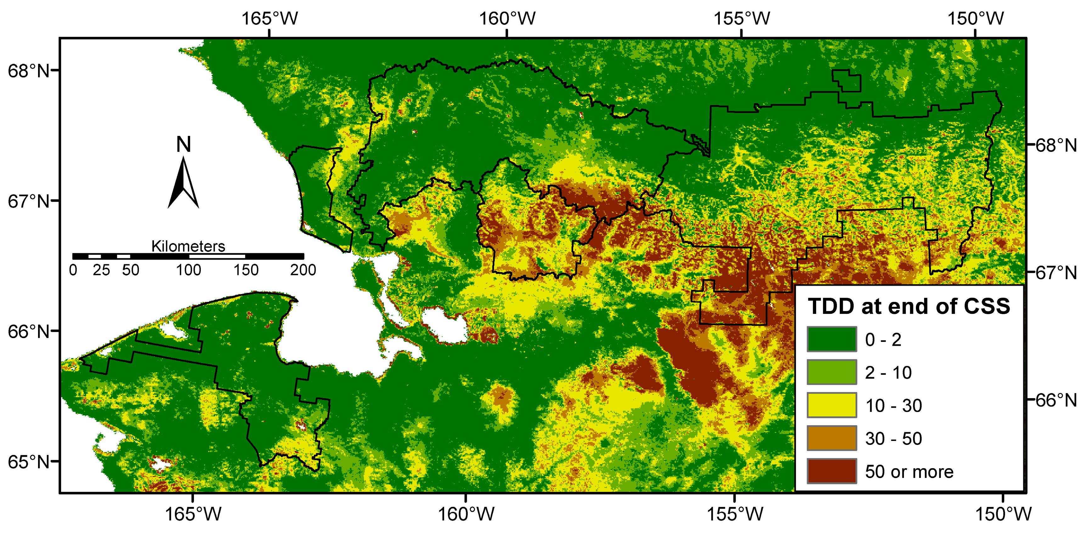
Over much of ARCN, the median end of the continuous snow season occurred when, on the average, few to no thaw degree-days had accumulated (Figure 6). In contrast, the forested lowlands in southern Kobuk Valley National Park (KOVA) and GAAR, and the south slopes of the mountains in KOVA, NOAT, and GAAR, have deeper snowpacks that required 50 or more thaw degree-days to melt. Our phenology cameras and temperature data show that indeed most of the thin tundra snowpack melts away during early spring days with above-freezing daily maximum temperatures but daily means near to freezing, while deep drifts persist into the summer [10].
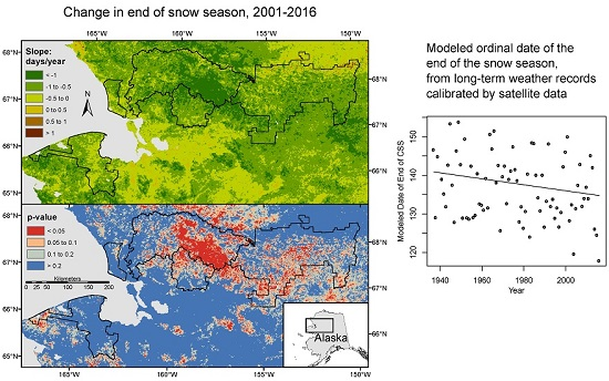
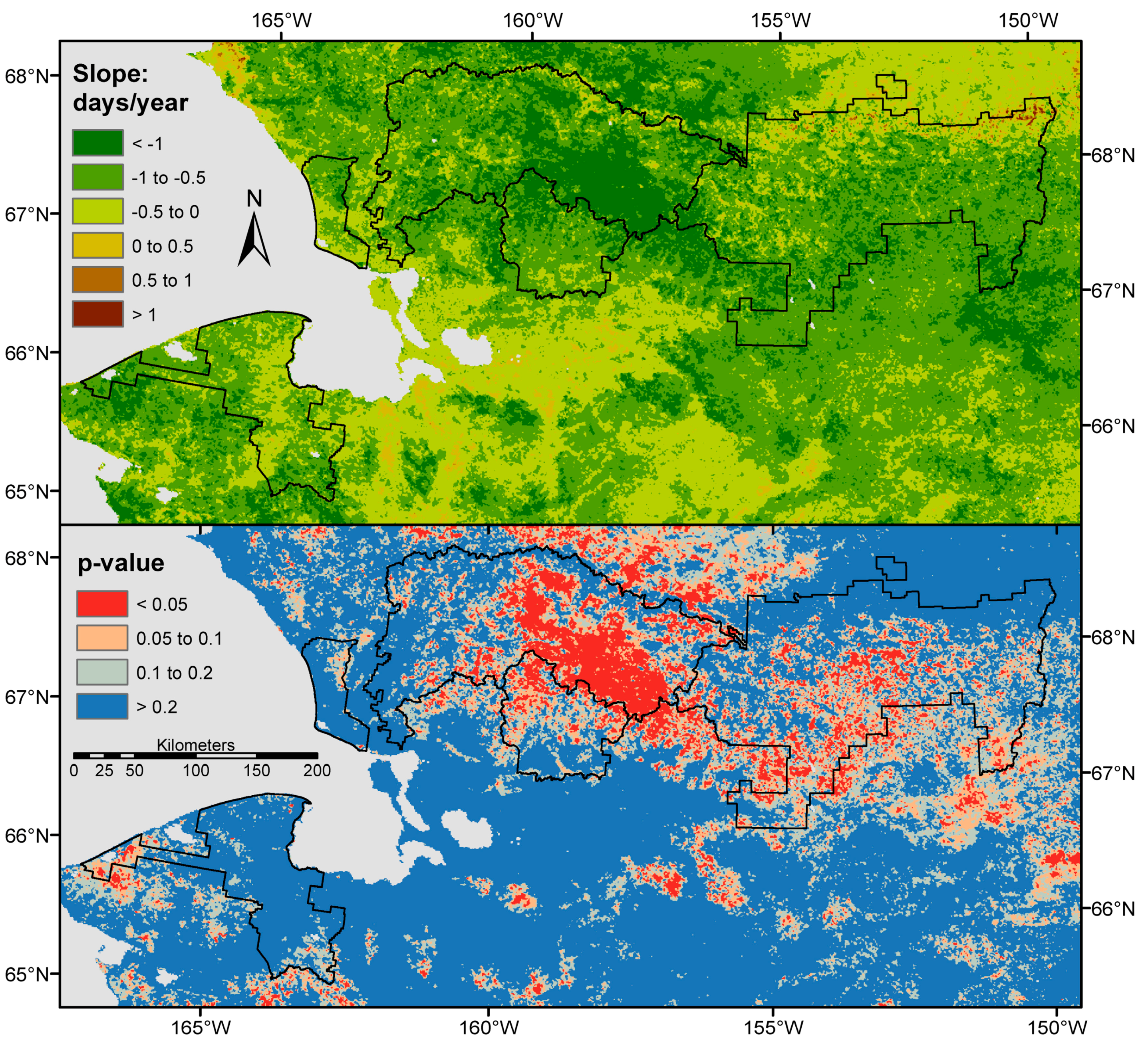
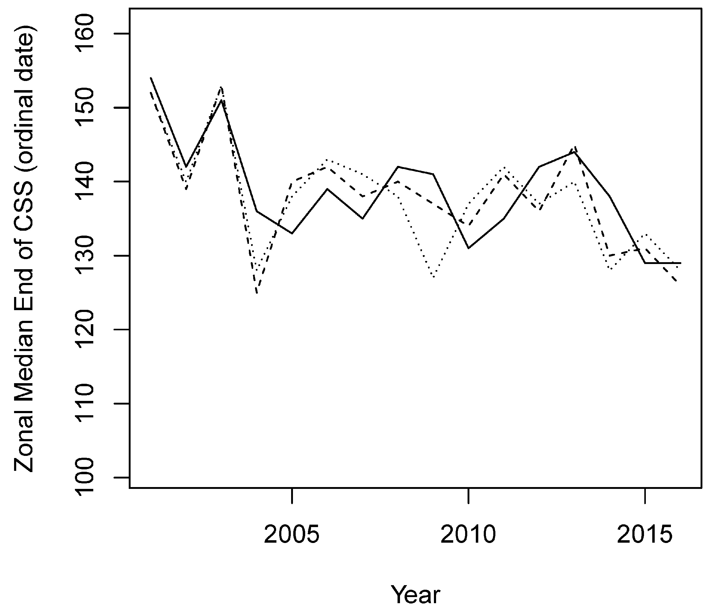
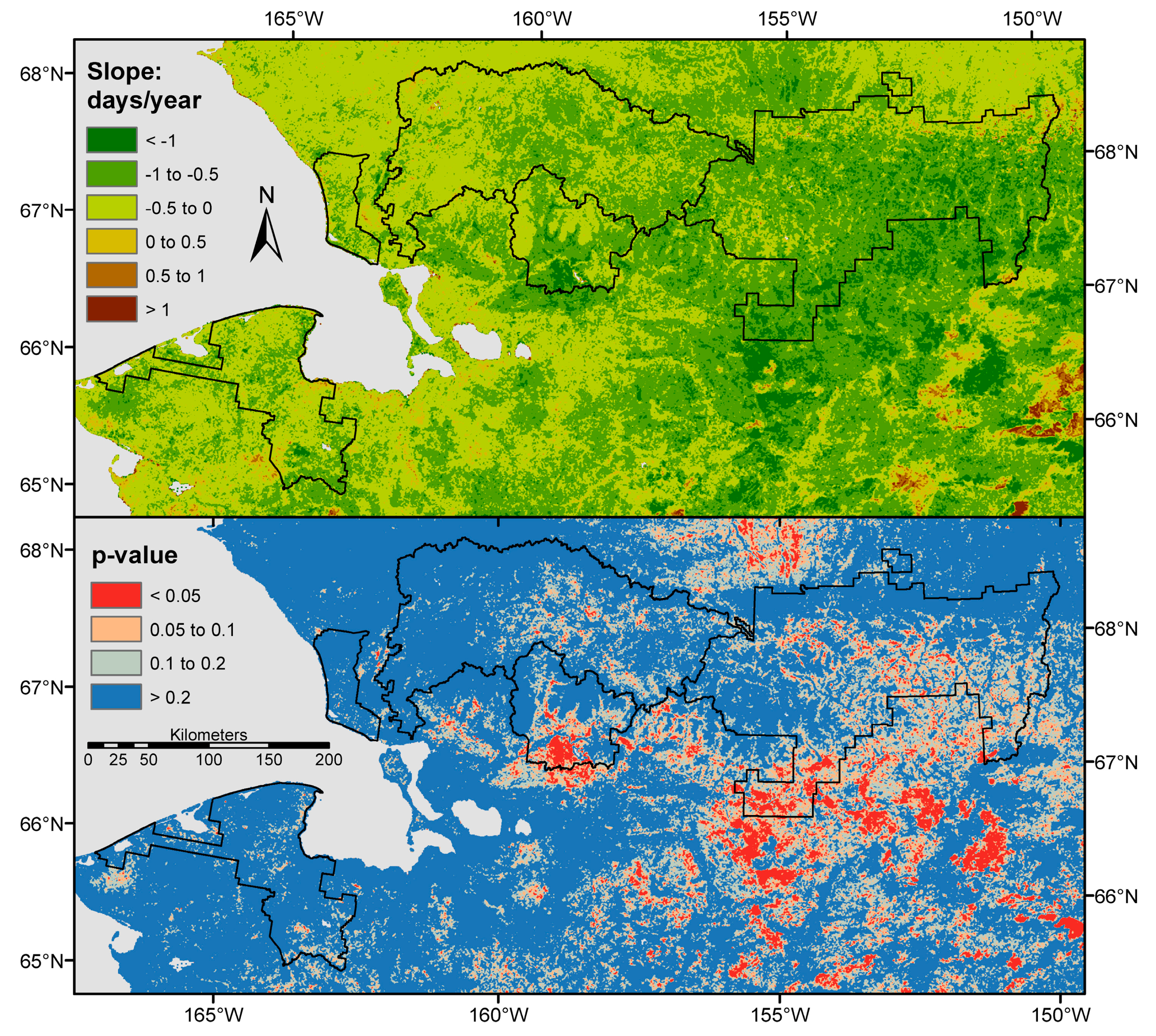
The Mann-Kendall trend test of the end of CSS from 2001 through 2016 showed a significant trend toward earlier snow-off in portions of the study area, mainly on the southern slopes of the Brooks Range and in the Noatak Valley (Figure 7). The median date of end of CSS is plotted in Figure 8 for the three ecozones that encompass most of the area with significant trends (zones I, M, and H of Figure 4). This plot shows two very late snow years near the beginning of the period of record (2001 and 2003), and a rather flat trend after 2003.
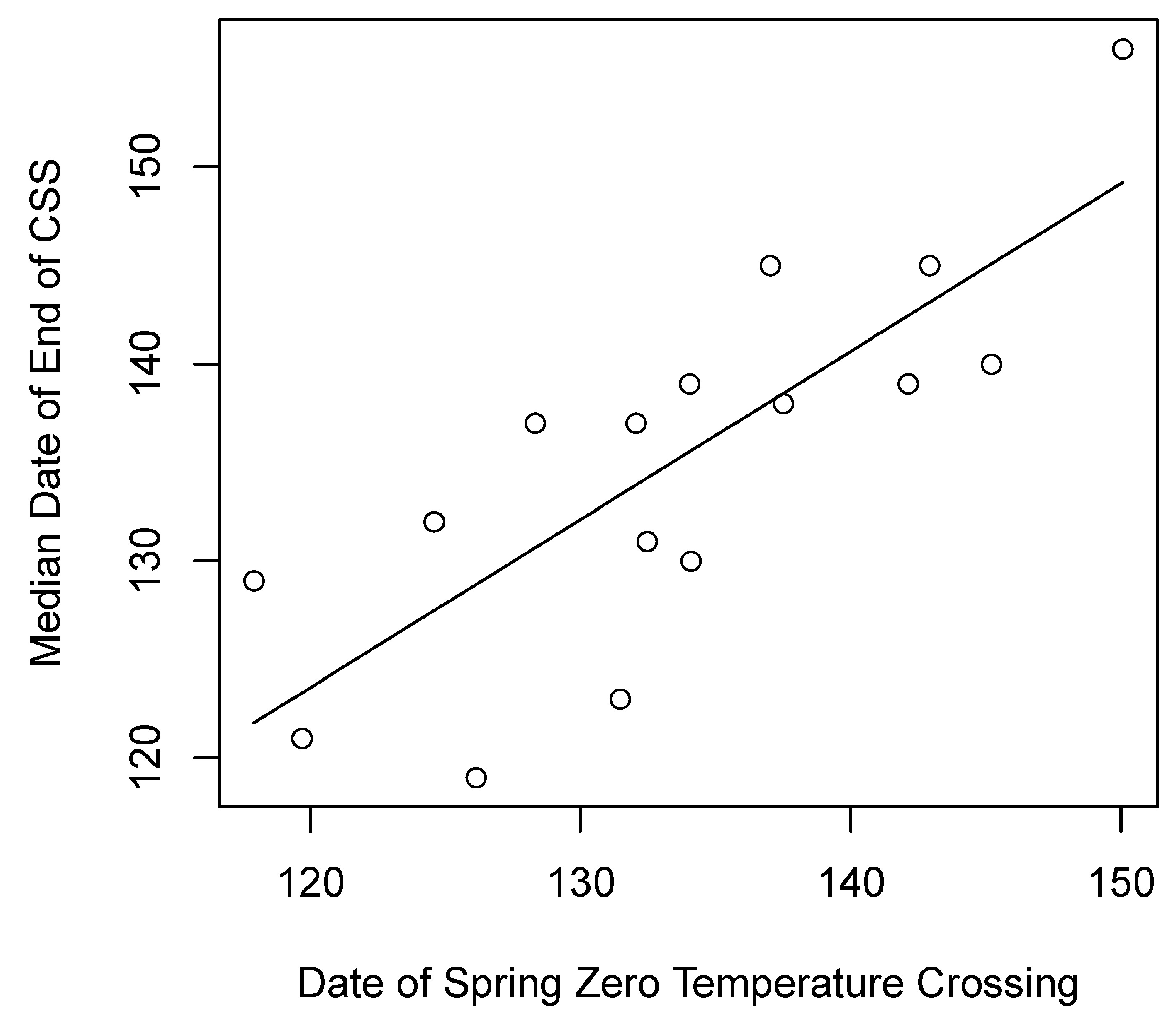
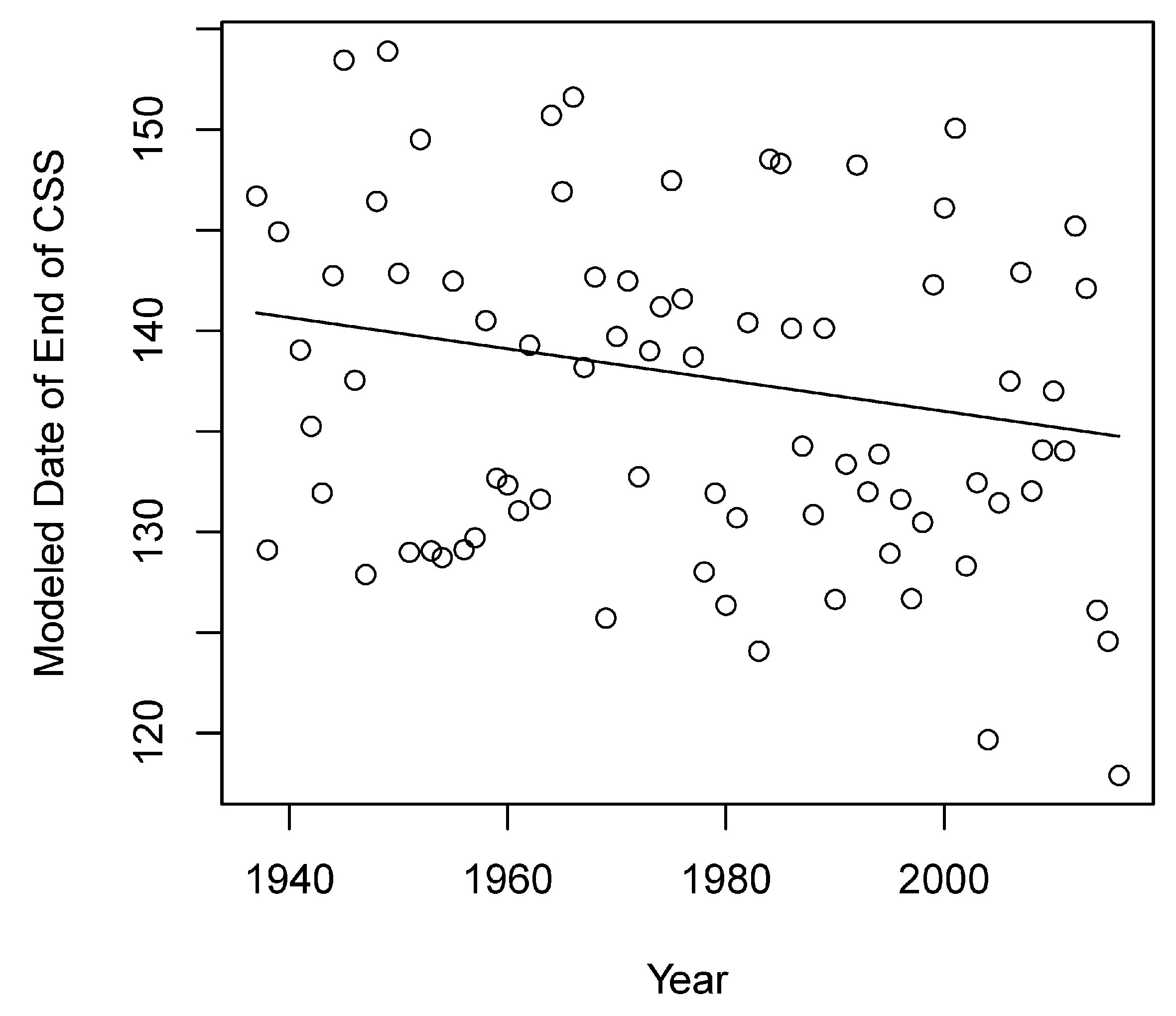
The long-term weather station at Kotzebue, Alaska showed highly significant correlations (p < 0.05) between the date when the interpolated plot of monthly average temperature crossed 0 °C and the median date at the end of CSS in all ten of the nearest ecological zones (for the years with MODIS data, 2001 through 2016). The zone with the closest match (as measured by lowest mean square difference between the date of zero crossing and the median date of the end of the CSS) was the extensive zone A in northern Bering Land Bridge National Preserve (BELA) (Figure 4 and Figure 9). If we use the regression in Figure 9 to predict the timing of snow-off in zone A from Kotzebue’s historical temperature data, we can reconstruct the timing of snow-off back to 1937 (Figure 10). These reconstructed dates show a year-to-year variability of 25 to 30 days, similar to the MODIS data (Figure 8). A simple linear trend line fitted to the reconstructed snow-off dates is significant (p = 0.02) with a slope of −0.78 days per decade. Thus, the average snow-off date in zone A is now about 6 days earlier than it was in 1937. Long-term weather records are also available for Bettles, Alaska (Figure 1), but most of the terrain within 150 km of this station has a significant snowpack and therefore it is not reasonable to neglect the thaw degree-days required to melt the snow as in the case of Kotzebue (Figure 6).
3.2. Spring Green-Up
The midpoints of spring green-up range from late May in low-elevation inland locations to late June at high elevations (Figure S4). A comparison of observations at remote automated cameras with the corresponding pixel values derived from MODIS (Figure 5) suggests a possible bias towards earlier dates from the MODIS data: the median difference MODIS date minus camera date was −6 days (n = 6). However, I would caution against drawing conclusions from just six verification points that involve comparing a small oblique camera scene with a single 250 m pixel.
The Mann-Kendall trend test for midpoint of green-up shows significant change to earlier green-up over the 16-year period in a rather small portion of ARCN (Figure 11). Significant trends toward earlier dates are most concentrated in the southern inland forested areas (ecozones K and N in Figure 4), where trends were driven by late springs in 2000 and 2001 (Figure 12).
Degradation of the MODIS Terra sensor over time [29] could possibly affect my observed trends in date of half-green-up (Figure 11). The effect of sensor degradation, estimated to be −0.001 to −0.004 NDVI units year−1 [29], on the green-up midpoint date depends on the slope of the annual NDVI curve. Green-up in our area requires 15 to 30 days [2], and, as will be reported below, typical NDVI maxima are around 0.8; this implies a spring NDVI change rate of 0.025 to 0.050 day−1. Thus an NDVI decline due to sensor degradation of −0.001 yr−1 would cause the observed green-up date to change between 0.001/0.050 = −0.02 day yr−1 and 0.001/0.025 = −0.04 day yr−1. The worst-case estimate of NDVI drift of −0.004 yr−1 [29] would produce a four-times greater change, −0.08 to −0.16 day yr−1. The rates of change associated with a significant Mann-Kendall test for change in the date of green-up are typically more negative than −1 day yr−1 (Figure 11). So the effect of sensor degradation is probably an order of magnitude less than the observed changes, and thus a minor factor. Sensor degradation may cause a slight underestimate of the area with a trend toward significantly earlier occurrence of spring green-up in Figure 11.
The long-term weather station at Kotzebue, Alaska showed highly significant correlations (p < 0.05) between the dates when all thaw degree-day values tested (60, 80, 100, … 220, 240 °C-days) were reached and the median date for midpoint of green-up in the four nearest ecological zones.
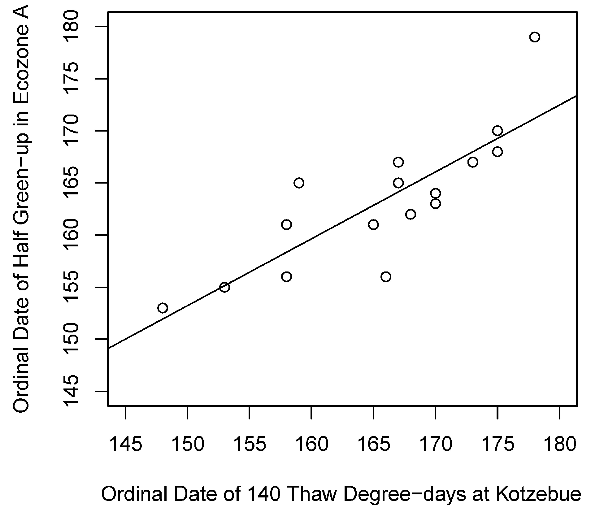
The best match was with the extensive ecozone A in northern coastal BELA and a degree-day threshold of 140 °C-days (Figure 13). If we use the regression in Figure 13 to predict the timing of green-up in ecozone A from historical temperature data from Kotzebue, we can reconstruct the timing of green-up back to 1937 (Figure 14). These reconstructed dates show a year-to-year variability of 20 to 25 days, similar to the MODIS data (Figure 12). A linear trend line fitted to these reconstructed green-up dates showed a highly significant (p = 0.009) regression slope of −0.80 days per decade, nearly identical to the slope of the change in snow-off date presented above. Thus, the average date of spring half green-up was also about 6 days earlier in 2015 than it was in 1937. Quantile regression [47,48] fitted to the 95th percentile values in Figure 14 suggests that the decline was steeper for years with late springs, about −1.25 days per decade. A similar reconstruction for eastern ARCN based on Bettles weather records was not attempted due to deeper snow in that area, as discussed above.
3.3. Maximum Greenness
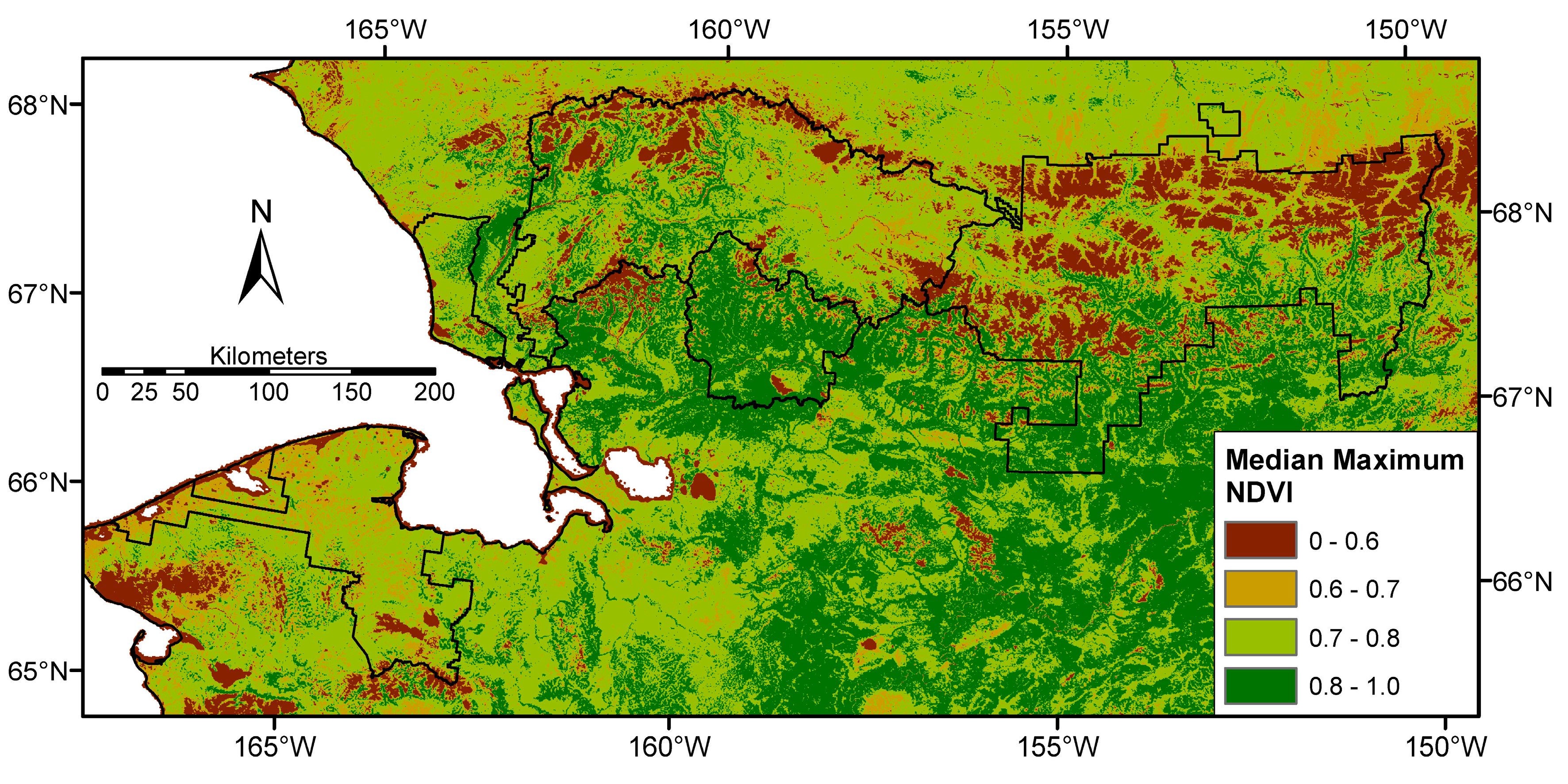
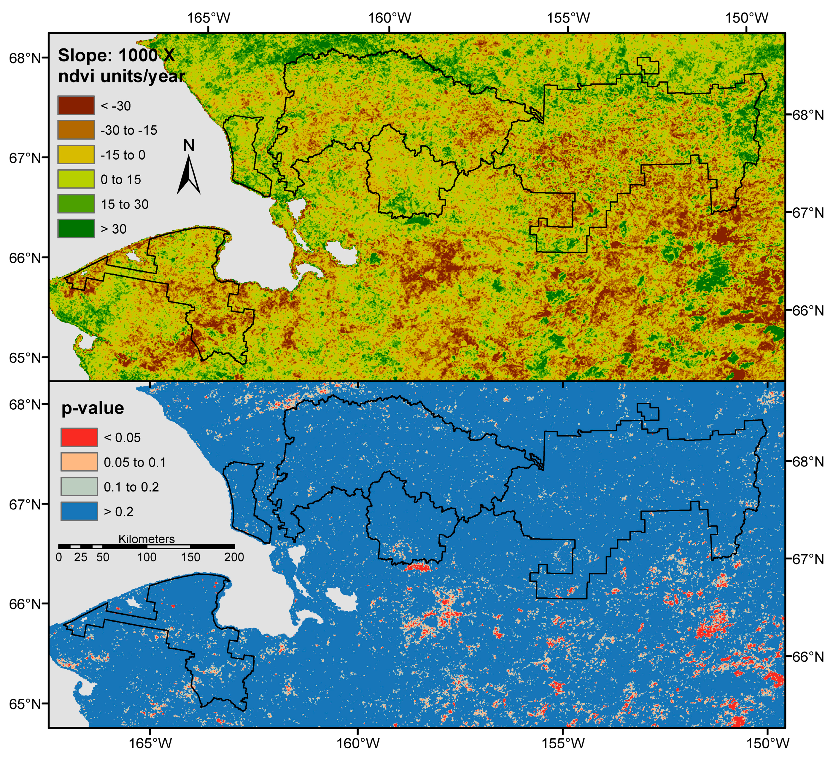
Maximum NDVI (Figure 15) is closely related to vegetation type (Figure 3): the lowest indices were in sparsely vegetated areas and the highest in forest, tall shrub, and some low-shrub tundra. Maximum NDVI was quite consistent from year to year: the coefficient of variation (standard deviation of NDVI divided by mean NDVI for 2000–2015, Figure S5) was less than 10% over most of ARCN. Maximum NDVI showed much weaker trends over the 16-year period than the spring phenological events discussed above (Figure 16). Few pixels had significant Mann-Kendall tests, and both positive and negative trends were present. This lack of trends stands in contrast to the longer-term greening trend visible from AVHRR (Advanced Very High Resolution Radiometer) satellite data since the 1980s [3,4,5,6,8]. The greening trend has recently slowed elsewhere in the Arctic, perhaps as a result of strengthened sea breezes that have depressed midsummer temperatures and increased cloudiness [5,6]. However, this explanation does not appear to apply in our study area, where July temperatures and annual sum of thaw degree-days showed a persistent long-term upward trend, even at the coast in Kotzebue (Figure 2). I would instead suggest that the addition of sufficient biomass to produce a significant trend in NDVI might require more time than is available in our 16-year dataset.
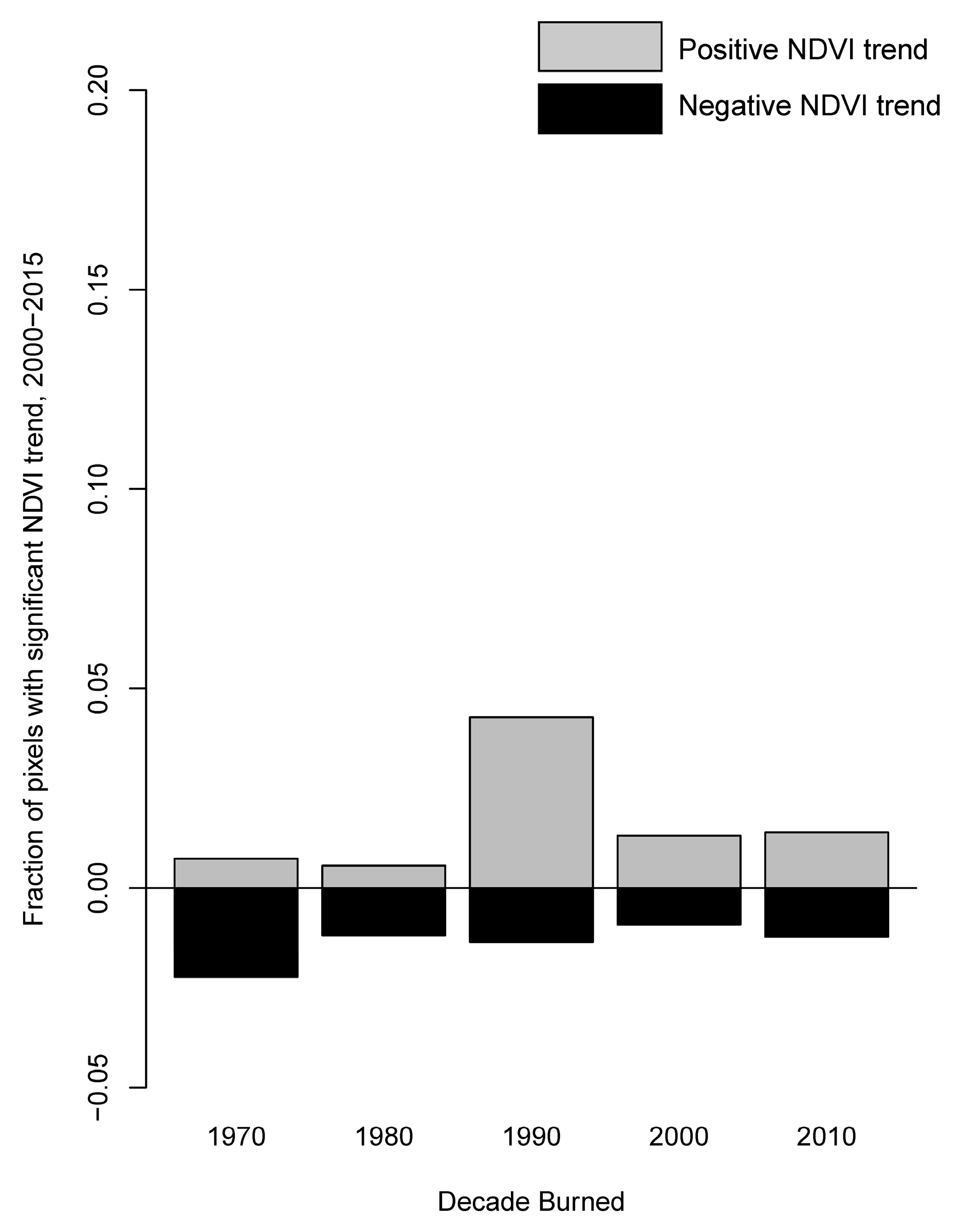
Several small areas with significant NDVI trend in BELA correspond to lakes that drained during the 1990 and 2000 decades [49] (Figure S6). Elsewhere in ARCN, areas with positive NDVI trends generally corresponded to perimeters of forest fires, i.e., areas undergoing post-fire plant succession. The area of strongly increasing NDVI just south of KOVA in Figure 16 is within the perimeter of a 1988 wildfire. Fire perimeters in southwestern GAAR from 1991 and 1997 also encircle areas of pixels with significant positive NDVI trends for 2000–2015 (Figure S7). In contrast, the extensive tundra lowlands of Cape Krusenstern National Monument (CAKR), BELA and NOAT lack positive NDVI trends, in spite of multiple large fires there in all decades since the 1970s. The relationships between maximum NDVI and fires are well illustrated if we extract all pixels in fire perimeters from the various decades and compute the proportion with significant (p < 0.05) Mann-Kendall test trends in maximum NDVI during 2000–2015 (Figure 17 and Figure 18). In GAAR and KOVA, where fires were predominantly in boreal forests, fire perimeters from the 1970s, 1980s, and 1990s show progressively more pixels with significantly positive trends in NDVI vs. time in 2000–2015 (Figure 17). In contrast, the predominantly tundra fires of BELA and NOAT appear to have little effect on recent NDVI trends: few pixels from fire perimeters of any decade had significant positive or negative NDVI trends in 2000–2015 (Figure 18).
The rate of change of NDVI in places with significant Mann-Kendall tests was more than +0.03 or less than −0.03 NDVI units year−1. This is an order of magnitude greater than the rate of NDVI change due to degradation of the Terra sensor (−0.001 to −0.004 NDVI units year−1 [29]). While the effect of sensor degradation on my results is probably minor, it may cause a slight underestimate of the area undergoing significant positive change in NDVI or a slight overestimate of the area undergoing significant negative change in NDVI.
3.4. Fall Senescence
The median midpoint of fall senescence by analysis of MODIS images ranged from late August in high-elevation areas to early October in lowland areas of the south and west (Figure S8). Observations of the midpoint of fall senescence at 5 remote camera sites from 2013 to 2015 yielded dates between 21 August and 16 September (ordinal dates 233 to 259) with none in late September or October (Figure 19). All of the corresponding pixel values for the senescence midpoint derived from MODIS were later than the camera observations, and the median difference (MODIS date minus camera date) was +17 days. The unexpectedly late senescence values obtained from the MODIS data have two probable causes: (1) fall phenology events are subject to a “late-bias,” because they are often sensed by the satellite well after they occur (due to cloudiness and low sun angles); (2) where vegetation is dominated by plants with weak or no senescence color changes (evergreen shrubs and coniferous trees, mosses, and lichens), the major fall change in satellite NDVI occurs with the arrival of snow, and not with changes in plant color that were analyzed at our camera locations.
Trends in the date of the MODIS-derived midpoint of fall senescence were weak over much of the study area (Figure S9). The relatively small areas with significant positive trends were driven by numerous suspect October senescence dates during years 2010–2014. Given the issues with sensing senescence described above, I would be reluctant to draw any conclusions about trends in the timing of senescence from these data.
I chose not to model the historical senescence dates using air temperature as I did for spring green-up. In addition to the questionable quality of the satellite senescence dates, multiple environmental factors affect fall senescence and confound its prediction from fall temperature data. These factors include the strong influence of photoperiod on senescence of some arctic shrubs (Betula nana [50]), the dependence of senescence on the timing of green-up [51], and also the effect of summer drought [52].
3.5. Establishment of the Continuous Snow Cover
The median date of the start of the continuous snow cover, based on the MODIS data, was in September at high elevations and October elsewhere, generally later in the west (Figure S10). Comparison of start of CSS as determined from automated cameras with the corresponding pixel values derived from MODIS showed a median difference (MODIS date minus camera data) of +4 days (Figure 19). There was good agreement for 9 of the 13 observations (4 days or less difference between the two data sources). The late-bias in the other 4 observations was probably due to the cloudiness and sun-angle issues discussed previously. Because a minority of observations appear to be affected by late bias, the median start of CSS (Figure S10) may be largely unaffected.
However, I suggest caution in accepting the apparent trend toward later snow cover establishment in CAKR and lowland areas of western NOAT during 2000–2015 (Figure S11), because this result could be produced by late-bias in a few years in the second half of the study time interval.
4. Conclusions
The MODIS Terra satellite has provided valuable insights into phenology trends in Alaska’s arctic National Parks. Both the end of the continuous snow season and the midpoint of spring green-up have become earlier in portions of the study area between 2000 and 2016. The strong relationship between spring phenology events (in tundra areas with minimal snowpacks) and thaw degree-days at a long-term weather station (Kotzebue) during the MODIS era (2000–2016) make it possible to extrapolate the snow-off and green-up dates with historic climate data back to 1937. This reconstruction suggests that the average date of both spring snow-off and green-up in tundra lowlands near Kotzebue have become earlier by about 6 days over this approximately 80-year time span, while the short-term year-to-year range is 20 to 30 days. The thin, windblown tundra snow cover type is widespread across the Arctic [53], thus it should be possible elsewhere to reconstruct snowmelt and green-up dates from long-term weather records calibrated by MODIS data.
In most areas the earlier spring green-ups since 2000 were not accompanied by a measurable increase in peak summer greenness over the same time interval. Other studies with longer timespans have detected overall arctic greening since the 1980s [3,4,5,6,8]. The lack of trend in maximum NDVI in my study area, in spite of continued gradual warming, may simply reflect the difficulty in discerning a very gradual trend in increasing arctic biomass from a relatively short time series. Localized significant greening over the 2000–2015 study period were observed in places where forest fires occurred during the 3 decades preceding the year 2000. Tundra fires and subsequent post-fire vegetation succession had little effect on greenness.
Fall phenology events (midpoint of fall senescence and establishment of snow cover) were difficult to sense by optical satellites in the Arctic, probably due to cloudiness and low sun angles during this time of year.
Supplementary Materials
The following are available online at www.mdpi.com/2072-4292/9/6/514/s1: Supplementary Materials.pdf. Supplementary Table S1 and captions for the Supplementary Figures S1 through S11. Table S1. Dates in the fall and spring when the solar zenith angle is less than 90°, 70°, and 80° at time of the MODIS Terra pass (10:30 am local time). Figure S1: Terrain shadowing in the study area under different sun angles. Figure S2. An example automated camera frame with analysis window outlined in red. Figure S3. Median for 2001–2016 of the ordinal date of the end of the continuous snow season (CSS). Figure S4. Median date of midpoint of spring green-up for years 2000–2015. Figure S5. Coefficient of variation in maximum NDVI, 2000–2015. Figure S6. Significance (Mann_Kendall test) of trend in maximum NDVI in BELA, 2000–2015 (upper) and 2002 Landsat image, color-infrared color scheme (lower). Figure S7. Trend of maximum NDVI in southwestern GAAR, 2000–2015. Figure S8. Median date of the midpoint of senescence, 2000–2015. Figure S9. Trend in the date of the midpoint of fall senescence for 2000–2015. Figure S10. Median date of the start of the continuous snow season (CSS), 2000–2015. Figure S11. Trend in the date of the establishment of the continuous snow season (CSS) 2000–2015.
Acknowledgments
This study and publications costs for open access were funded by the National Park Service, Inventory and Monitoring Program, Arctic Network. Contributions by the Geographic Network for Alaska, University of Alaska, Fairbanks were under CESU agreement P13AC00836, funded by the National Park Service. Thanks to Ken Hill and Pam Sousanes for installation and management of the ARCN remote automated cameras.
Conflicts of Interest
The author declares no conflict of interest. The technical committee for the NPS Arctic Inventory and Monitoring Network, and the author’s NPS supervisor, approved the plan for this study, including the decision to publish. The remote sensing data used in this study are all from public sources. The author was responsible for all analysis, and writing of the manuscript.
References
- Overland, J.; Hanna, E.; Hanssen-Bauer, I.; Kim, S.-J.; Walsh, J.; Wang, M.; Bhatt, U.S. Air temperature. Bull. Am. Meteorol. Soc. 2015, 96, S128–S129. [Google Scholar]
- Derksen, C.; Brown, R. Spring snow cover extent reductions in the 2008–2012 period exceeding climate model projections. Geophys. Res. Lett. 2012, 39, L19504. [Google Scholar] [CrossRef]
- Jia, G.J.; Epstein, H.E.; Walker, D.A. Greening of arctic Alaska, 1981–2001. Geophys. Res. Lett. 2003, 30, 2067. [Google Scholar] [CrossRef]
- Verbyla, D. The greening and browning of Alaska based on 1982–2003 satellite data. Glob. Ecol. Biogeogr. 2008, 17, 547–555. [Google Scholar] [CrossRef]
- Bhatt, U.S.; Walker, D.A.; Raynolds, M.K.; Bieniek, P.A.; Epstein, H.E.; Comiso, J.C.; Pinzon, J.E.; Tucker, C.J.; Polyakov, I.V. Recent declines in warming and vegetation greening trends over pan-Arctic tundra. Remote Sens. 2013, 5, 4229–4254. [Google Scholar] [CrossRef]
- Bieniek, P.A.; Bhatt, U.S.; Walker, D.A.; Raynolds, M.K.; Comiso, J.C.; Epstein, H.E.; Pinzon, J.E.; Tucker, C.J.; Thoman, R.L.; Tran, H.; et al. Climate Drivers Linked to Changing Seasonality of Alaska Coastal Tundra Vegetation Productivity. Earth Interact. 2015, 19, 1–29. [Google Scholar] [CrossRef]
- Lawler, J.P.; Miller, S.D.; Sanzone, D.; Ver Hoef, J.; Young, S.B. Arctic Network Vital Signs Monitoring Plan; Natural Resource Report NPS/ARCN/NRR-2009/088; National Park Service: Fort Collins, CO, USA, 2009. Available online: https://irma.nps.gov/DataStore/Reference/Profile/661340 (accessed on 18 May 2017).
- Swanson, D.K. Satellite Greenness Data Summary for the Arctic Inventory and Monitoring Network, 1990–2009; Natural Resource Data Series NPS/ARCN/NRDS—2010/124; National Park Service: Fort Collins, CO, USA, 2010. Available online: https://irma.nps.gov/DataStore/Reference/Profile/2166935 (accessed on 18 May 2017).
- Swanson, D.K. Snow Cover Monitoring with MODIS Satellite Data in the Arctic Inventory and Monitoring Network, Alaska, 2000–2013; Natural Resource Data Series NPS/ARCN/NRDS—2014/634; National Park Service: Fort Collins, CO, USA, 2014. Available online: https://irma.nps.gov/App/Reference/Profile/2208992 (accessed on 18 May 2017).
- Swanson, D.K. Monitoring of Greenness and Snow Phenology by Remote Automated Cameras in the NPS Arctic Inventory and Monitoring Network, 2013-14; Natural Resource Data Series NPS/ARCN/NRDS—2015/798; National Park Service: Fort Collins, CO, USA, 2015. Available online: https://irma.nps.gov/DataStore/Reference/Profile/2222147 (accessed on 18 May 2017).
- MODIS Land Team MODIS Land. Available online: https://modis-land.gsfc.nasa.gov/ (accessed on 6 December 2016).
- PRISM Climate Group. Mean Monthly Temperature for Alaska 1971–2000, Annual Mean Average Temperature for Alaska 1971–2000. Oregon State University: Corvallis, OR, USA. Available online: http://prism.oregonstate.edu (accessed on 8 September 2014).
- Barrett, R.T.S.; Hollister, R.D.; Oberbauer, S.F.; Tweedie, C.E. Arctic plant responses to changing abiotic factors in northern Alaska. Am. J. Bot. 2015, 102, 2020–2031. [Google Scholar] [CrossRef] [PubMed]
- NOAA Regional Climate Centers Applied Climate Information System (ACIS). Available online: http://xmacis.rcc-acis.org/ (accessed on 21 October 2016).
- Jorgenson, M.T.; Roth, J.E.; Miller, P.F.; Macander, M.J.; Duffy, M.S.; Wells, A.F.; Frost, G.V.; Pullman, E.R. An Ecological Land Survey and Landcover Map of the Arctic Network; Natural Resource Technical Report ARCN/NRTR—2009/270; National Park Service: Fort Collins, CO, USA, 2009. Available online: https://irma.nps.gov/App/Reference/Profile/663934 (accessed on 18 May 2017).
- Hall, D.K.; Riggs, G.A.; Salomonson, V.V. Data Set Documentation: MODIS/Terra Snow Cover Daily L3 Global 500 m Grid, Version 5. Available online: http://nsidc.org/data/docs/daac/modis_v5/mod10a1_modis_terra_snow_daily_global_500m_grid.gd.html (accessed on 6 December 2016).
- Hall, D.K.; Salomonson, V.V.; Riggs, A. MODIS/Terra Snow Cover Daily L3 Global 500 m Grid, Version 5; Snow and Ice Data Center Distributed Active Archive Center: Boulder, Colorado, USA, 2006; Available online: http://dx.doi.org/10.5067/63NQASRDPDB0 (accessed on 11 February 2016).
- Riggs, G.A.; Hall, D.K.; Salomonson, V.V. MODIS Snow Products User Guide to Collection 5; Snow and Ice Data Center Distributed Active Archive Center: Boulder, Colorado, USA, 2006; Available online: http://nsidc.org/data/docs/daac/modis_v5/dorothy_snow_doc.pdf (accessed on 11 February 2016).
- Lindsay, C.; Zhu, J.; Miller, A.E.; Kirchner, P.; Wilson, T.L. Deriving Snow Cover Metrics for Alaska from MODIS. Remote Sens. 2015, 7, 12961–12985. [Google Scholar] [CrossRef]
- Zhu, J.; Lindsay, C. MODIS-Derived Snow Metrics Algorithm, Version 1.1; University of Alaska Fairbanks, Geographic Information Network for Alaska: Fairbanks, AK, USA, 2013; Available online: http://www.gina.alaska.edu/projects/modis-derived-ndvi-metrics (accessed on 16 May 2014).
- Geographic Information Network for Alaska. Projects—MODIS-Derived Snow Metrics—Geographic Information Network of Alaska. Available online: http://www.gina.alaska.edu/projects/modis-derived-snow-metrics (accessed on 1 December 2016).
- Jenkerson, C.; Maiersperger, T.; Schmidt, G. eMODIS: A User-Friendly Data Source; US Geological Survey: Reston, VA, USA, 2010. Available online: http://pubs.er.usgs.gov/usgspubs/ofr/ofr20101055 (accessed on 11 February 2016).
- Jenkerson, C.B.; Schmidt, G.L. eMODIS Alaska. In Proceedings of the American Society for Photogrammetry & Remote Sensing Annual Conference (ASPRS) 2009 Annual Conference, Baltimore, MD, USA, 9–13 March 2009; Available online: http://info.asprs.org/publications/proceedings/baltimore09/0043.pdf (accessed on 11 February 2016).
- U.S. Geological Survey. EarthExplorer. Available online: http://earthexplorer.usgs.gov/ (accessed on 6 December 2016).
- Swets, D.L.; Reed, B.C.; Rowland, J.D.; Marko, S.E. A weighted least-squares approach to temporal NDVI smoothing. In Proceedings of the 1999 ASPRS Annual Conference: From Image to Information, Portland, OR, USA, 17–21 May 1999; American Society for Photogrammetry and Remote Sensing: Bethesda, MD, USA, 1999; pp. 526–536. [Google Scholar]
- Reed, B.C.; Brown, J.F.; VanderZee, D.; Loveland, T.R.; Merchant, J.W.; Ohlen, D.O. Measuring phenological variability from satellite imagery. J. Veg. Sci. 1994, 5, 703–714. [Google Scholar] [CrossRef]
- Zhu, J.; Miller, A.E.; Lindsay, C.; Broderson, D.; Heinrichs, T.; Martyn, P. MODIS NDVI Products and Metrics User Manual, Version 1.0; Geographic Information Network for Alaska, University of Alaska: Fairbanks, AK, USA, 2013. [Google Scholar]
- Geographic Information Network of Alaska Projects—MODIS-Derived NDVI Metrics—Geographic Information Network of Alaska. Available online: http://www.gina.alaska.edu/projects/modis-derived-ndvi-metrics (accessed on 1 December 2016).
- Wang, D.; Morton, D.; Masek, J.; Wu, A.; Nagol, J.; Xiong, X.; Levy, R.; Vermote, E.; Wolfe, R. Impact of sensor degradation on the MODIS NDVI time series. Remote Sens. Environ. 2012, 119, 55–61. [Google Scholar] [CrossRef]
- R Core Team. R: A Language and Environment for Statistical Computing, Version 3.0.1; R Foundation for Statistical Computing: Vienna, Austria, 2014; Available online: http://www.R-project.org (accessed on 21 January 2014).
- Hijmans, R.J. Raster: Geographic Data Analysis and Modeling, R Package Version 2.3-40; R Foundation for Statistical Computing: Vienna, Austria, 2015; Available online: http://CRAN.R-project.org/package=raster (accessed on 4 January 2016).
- Bivand, R.; Keitt, T.; Rowlingson, B. Rgdal: Bindings for the Geospatial Data Abstraction Library, R Package Version 0.9-2; R Foundation for Statistical Computing: Vienna, Austria, 2015; Available online: http://CRAN.R-project.org/package=rgdal (accessed on 4 January 2016).
- Swanson, D.K. Landscape Patterns and Dynamics Monitoring Protocol for the Arctic Network: Narrative; Natural Resource Report NPS/ARCN/NRR—2017/1380; National Park Service: Fort Collins, CO, USA, 2017. Available online: https://irma.nps.gov/DataStore/Reference/Profile/2238342 (accessed on 18 May 2017).
- Swanson, D.K. Landscape Patterns and Dynamics Monitoring Protocol for the Arctic Network: Standard Operating Procedures; Natural Resource Report NPS/ARCN/NRR—2017/1381; National Park Service: Fort Collins, CO, USA, 2017. Available online: https://irma.nps.gov/DataStore/Reference/Profile/2238343 (accessed on 18 May 2017).
- Boggs, K.; Michaelson, J. Ecological Subsections of Gates of the Arctic National Park and Preserve; Inventory and Monitoring Program; National Park Service, Alaska Region: Anchorage, AK, USA, 2001. Available online: https://irma.nps.gov/App/Reference/DownloadDigitalFile?code=151098&file=GAAR_EcologicalSubs_final.pdf (accessed on 18 May 2017).
- Jorgenson, M.T. Ecological Subsections of Bering Land Bridge National Preserve; Inventory and Monitoring Program; National Park Service, Alaska Region: Anchorage, AK, USA, 2001. Available online: https://irma.nps.gov/App/Reference/DownloadDigitalFile?code=418816&file=BELA_EcologicalSubsections.pdf (accessed on 18 May 2017).
- Jorgenson, M.T.; Swanson, D.K.; Macander, M. Landscape-Level Mapping of Ecological Units for the Noatak National Preserve, Alaska; Inventory and Monitoring Program; National Park Service, Alaska Region: Anchorage, AK, USA, 2001. Available online: https://irma.nps.gov/App/Reference/DownloadDigitalFile?code=419154&file=NOAT_EcologicalSubsections.pdf (accessed on 18 May 2017).
- Swanson, D.K. Ecological Units of Cape Krusenstern National Monument, Alaska; Inventory and Monitoring Program; National Park Service, Alaska Region: Anchorage, AK, USA, 2001. Available online: https://irma.nps.gov/App/Reference/Profile/584437 (accessed on 18 May 2017).
- Swanson, D.K. Ecological Units of Kobuk Valley National Park, Alaska; Inventory and Monitoring Program; National Park Service, Alaska Region: Anchorage, AK, USA, 2001. Available online: https://irma.nps.gov/App/Reference/Profile/584437 (accessed on 18 May 2017).
- Molau, U.; Nordenhall, U.; Eriksen, B. Onset of flowering and climate variability in an alpine landscape: A 10-year study from Swedish Lapland. Am. J. Bot. 2005, 92, 422–431. [Google Scholar] [CrossRef] [PubMed]
- Richardson, A.D.; Jenkins, J.P.; Braswell, B.H.; Hollinger, D.Y.; Ollinger, S.V.; Smith, M.-L. Use of digital webcam images to track spring green-up in a deciduous broadleaf forest. Oecologia 2007, 152, 323–334. [Google Scholar] [CrossRef] [PubMed]
- Sonnentag, O.; Hufkens, K.; Teshera-Sterne, C.; Young, A.M.; Friedl, M.; Braswell, B.H.; Milliman, T.; O’Keefe, J.; Richardson, A.D. Digital repeat photography for phenological research in forest ecosystems. Agric. For. Meteorol. 2012, 152, 159–177. [Google Scholar] [CrossRef]
- Helsel, D.R.; Hirsch, R.M. Trend analysis. In Statistical Methods in Water Resources Techniques of Water Resources Investigations, Book 4, Chapter A3; U.S. Geological Survey: Reston, VA, USA, 2002; pp. 323–356. [Google Scholar]
- Sen, P.K. Estimates of the regression coefficient based on Kendall’s tau. J. Am. Stat. Assoc. 1968, 63, 1379–1389. [Google Scholar] [CrossRef]
- Marchetto, A. Rkt: Mann-Kendall Test, Seasonal and Regional Kendall Tests; R Package Version 1.4; R Foundation for Statistical Computing: Vienna, Austria, 2015; Available online: http://CRAN.R-project.org/package=rkt (accessed on 5 November 2015).
- Alaska Interagency Coordination Center. Fire History in Alaska. Available online: http://afsmaps.blm.gov/imf_firehistory/imf.jsp?site=firehistory (accessed on 28 June 2016).
- Koenker, R.; Bassett, G., Jr. Regression quantiles. Econometrica 1978, 46, 33–50. [Google Scholar] [CrossRef]
- Koenker, R. Package “Quantreg” Version 5.26; R Foundation for Statistical Computing: Vienna, Austria, 2016; Available online: https://cran.r-project.org/web/packages/quantreg/quantreg.pdf (accessed on 28 June 2016).
- Swanson, D.K. Surface Water Area Change in the Arctic Network of National Parks, Alaska, 1985–2011: Analysis of Landsat Data; Natural Resource Data Series NPS/ARCN/NRDS—2013/445; National Park Service: Fort Collins, CO, USA, 2013. Available online: https://irma.nps.gov/App/Reference/Profile/2193078 (accessed on 18 May 2017).
- Biebl, R. Influence of short-days on arctic plants during the arctic long-days. Planta 1967, 75, 77–84. [Google Scholar] [CrossRef] [PubMed]
- Oberbauer, S.F.; Elmendorf, S.C.; Troxler, T.G.; Hollister, R.D.; Rocha, A.V.; Bret-Harte, M.S.; Dawes, M.A.; Fosaa, A.M.; Henry, G.H.R.; Høye, T.T.; et al. Phenological response of tundra plants to background climate variation tested using the International Tundra Experiment. Philos. Trans. R. Soc. Lond. B Biol. Sci. 2013, 368, 13–20. [Google Scholar] [CrossRef] [PubMed]
- Marchand, F.L.; Verlinden, M.; Kockelbergh, F.; Graae, B.J.; Beyens, L.; Nijs, I. Disentangling effects of an experimentally imposed extreme temperature event and naturally associated desiccation on Arctic tundra. Funct. Ecol. 2006, 20, 917–928. [Google Scholar] [CrossRef]
- Sturm, M.; Holmgren, J.; Liston, G.E. A Seasonal Snow Cover Classification System for Local to Global Applications. J. Clim. 1995, 8, 1261–1283. [Google Scholar] [CrossRef]
Figure 1.
The five National Park Service (NPS) units that form the Arctic Inventory and Monitoring Network (ARCN): Bering Land Bridge National Preserve (BELA), Cape Krusenstern National Monument (CAKR), Gates of the Arctic National Park and Preserve (GAAR), Kobuk Valley National Park (KOVA), and Noatak National Preserve (NOAT). Shown also are the five remote automated camera locations (asterisks), and the long-term weather stations of Kotzebue and Bettles.

Figure 2.
Mean July temperatures (upper) and annual sum of thaw degree-days (lower) at Kotzebue, Alaska 1937–2016. National Weather Service data from [14]. The trend lines are linear regressions: y = −22.71 + 0.0177x, r2 = 0.06, p = 0.02 for July temperature and y = −4385 + 2.757x, r2 = 0.19, p < 0.001 for thaw degree days.

Figure 3.
The general vegetation of the study area, simplified from [15].
Figure 3.
The general vegetation of the study area, simplified from [15].

Figure 4.
Ecological zones used to summarize phenology data in ARCN. These zones were aggregated from ecological subsections [35,36,37,38,39] to obtain 2 to 4 coherent zones per NPS unit.
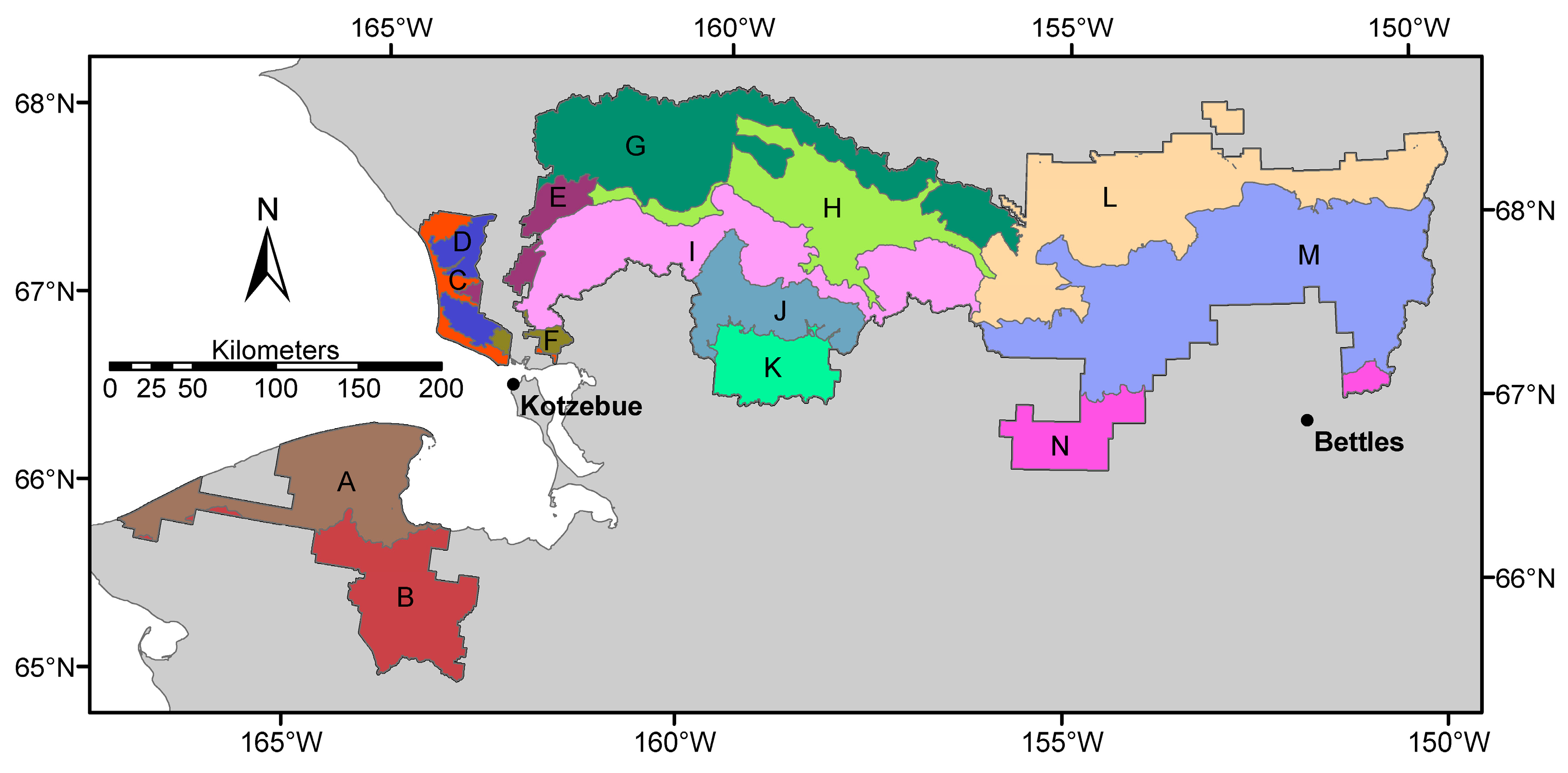
Figure 5.
Plot of the ordinal date for the end of the continuous snow season (CSS) and midpoint of spring green-up by ground camera (x) vs. satellite data analysis (y). The solid line marks an exact match between the two data sources, while the dashed lines mark where the satellite data were 20 days earlier (lower) or later (upper) than the ground camera data.

Figure 6.
Thaw degree-days (TDD) accumulated by the end of the continuous snow season (CSS), from overlay of the median date of end of CSS (Figure S3) on long-term average monthly temperature data by [12].

Figure 7.
Trend in the end of continuous snow season (CSS) for 2001–2016. The upper map is Theil-Sen’s slope for ordinal day of the end of the CSS vs. year. The lower map is the Mann-Kendall two-tailed test p-value for this trend. Both maps had 500 m resolution, smoothed for display with a 3-by-3 median filter.

Figure 8.
Median end of the continuous snow season (CSS) in the three ecological zones with the highest density of pixels with a significant trend (Figure 11). These are zones I (dashed line), H (dotted line), and M (solid line) of Figure 4. Linear regressions through these points (not shown) have fairly low p-values (zone I p = 0.09, zone H p = 0.05, zone M p = 0.06) and have slopes of −4.5, −5.1, and −5.0 days/decade, respectively.

Figure 9.
Plot of the median date of the end of the continuous snow season (CSS) in ecological zone A vs. the date in the spring when the temperature crosses 0 °C (as determined from a plot of monthly means) at Kotzebue, Alaska for years 2001–2015. The trend line is a linear regression y = 21.1 + 0.85x, r2 = 0.63, p = 0.0003.

Figure 10.
Modeled dates of snow-off in ecological zone A. The regression from Figure 9 was applied to weather records from Kotzebue, Alaska to reconstruct the date of the end of the continuous snow season in ecological zone A for each year back to 1937 (the points). The solid line is the long-term trend with time through the points, from linear regression, y = 291.3 − 0.078x, r2 = 0.06, p = 0.02. This is simply a linear transformation of the underlying decline in date of the spring zero crossing date over time, which has a similar regression (y = 316.6 − 0.091x, r2 = 0.06, p = 0.02).

Figure 11.
Trend in the date of the midpoint of spring green-up for 2000–2015. The upper map is Theil-Sen’s slope for ordinal day of the midpoint of spring green-up vs. year. The lower map is the Mann-Kendall test p-value for this trend (two-tailed test). Both maps had 250 m resolution, smoothed for display with a 5-by-5 median filter.

Figure 12.
Median midpoint by year of spring green-up for the two ecological zones (zone K—dashed line and zone N—solid line) with the highest density of pixels with significant trend as shown in Figure 11. Linear regressions through the points (not shown) are significant (p = 0.04 and 0.02, for zones K and N, respectively) and have slopes of −3.2 (zone K) and −4.3 (zone N) days per decade.
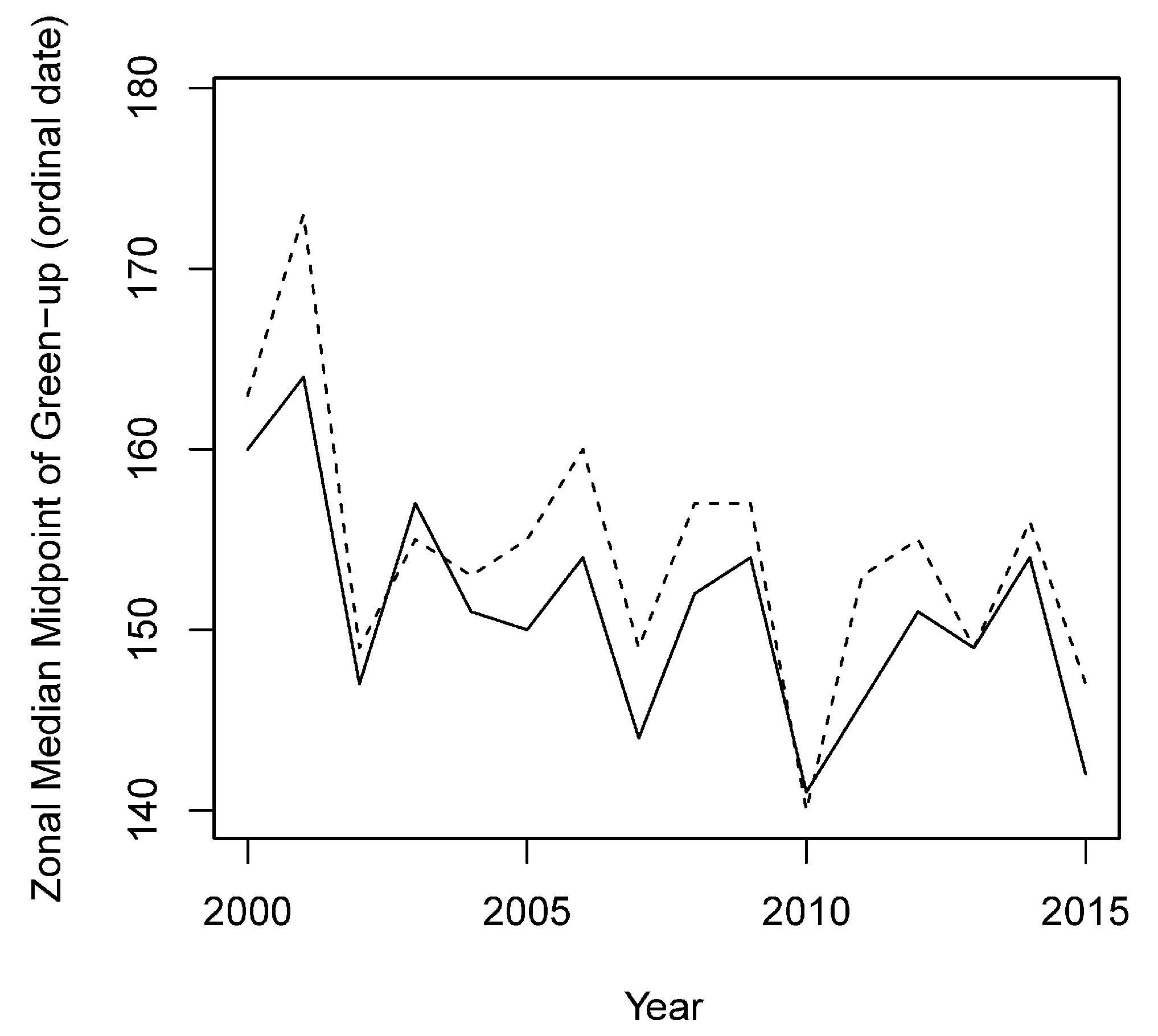
Figure 13.
Plot of the median ordinal date of half-greenup in ecozone A vs. the ordinal date of 140 thaw degree-days at Kotzebue, Alaska, as computed from monthly means. The trend line is a linear regression y = 56.9411 + 0.6419x, r2 = 0.68, p < 0.001.
Figure 13.
Plot of the median ordinal date of half-greenup in ecozone A vs. the ordinal date of 140 thaw degree-days at Kotzebue, Alaska, as computed from monthly means. The trend line is a linear regression y = 56.9411 + 0.6419x, r2 = 0.68, p < 0.001.

Figure 14.
Modeled dates of spring half-greenup in ecozone A. The regression between thaw degree-days in Kotzebue, Alaska and date of half green-up from Figure 13 was used to model the spring half-green-up for each year using historical weather records back to 1937 (points). The solid line is a linear regression y = 323.2 − 0.080x, r2 = 0.09, p = 0.009. The dashed line is a quantile regression with tau of 0.95, an estimate of the trend in the 95th percentile values [47,48], y = 420.9 − 0.125x.

Figure 15.
Median maximum normalized difference vegetation index (NDVI), 2000–2015.

Figure 16.
Trend of maximum NDVI for 2000–2015. The upper map is Theil-Sen’s slope of maximum NDVI vs. year. Brown indicates decreasing and green an increasing NDVI over time. The lower map is the Mann-Kendall test of significance of the trend (two-tailed test).
Figure 16.
Trend of maximum NDVI for 2000–2015. The upper map is Theil-Sen’s slope of maximum NDVI vs. year. Brown indicates decreasing and green an increasing NDVI over time. The lower map is the Mann-Kendall test of significance of the trend (two-tailed test).

Figure 17.
Fraction of pixels with significant trends in maximum NDVI during the period 2000–2015, for pixels within perimeters of fires from various decades in GAAR and KOVA. Most fire area here is within the boreal forest. The gray-shaded bars give the proportion of all pixels with significant (p < 0.05) positive NDVI trends, and the black bars are the proportion of significant (p < 0.05) negative NDVI trends, by the Mann-Kendall test on annual maximum NDVI for the period 2000–2015.
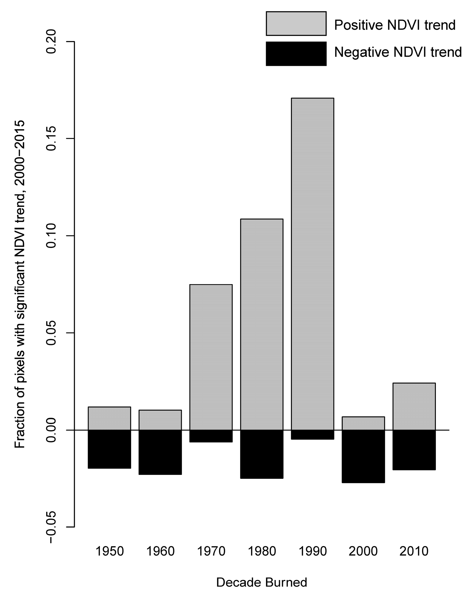
Figure 18.
Fraction of pixels with significant trends in maximum NDVI during the period 2000–2015, for pixels within perimeters of fires from various decades in BELA and NOAT. Most fire area here is in tundra vegetation. The gray-shaded bars give the proportion of all pixels with significant (p < 0.05) positive NDVI trends and the black bars are the proportion of significant (p < 0.05) negative NDVI trends, by the Mann-Kendall test on annual maximum NDVI for the period 2000–2015. The vertical scale is the same as in Figure 17.

Figure 19.
Plot of the ordinal date of the midpoint of fall senescence and the start of the continuous snow season (CSS) by ground camera (x) vs. satellite data analysis (y). The solid line marks an exact match between the two data sources, while the dashed lines mark where the satellite data are 20 days earlier (lower) or later (upper) than the ground camera data.

© 2017 by the author. Licensee MDPI, Basel, Switzerland. This article is an open access article distributed under the terms and conditions of the Creative Commons Attribution (CC BY) license (http://creativecommons.org/licenses/by/4.0/).
Share and Cite
MDPI and ACS Style
Swanson, D.K. Trends in Greenness and Snow Cover in Alaska’s Arctic National Parks, 2000–2016. Remote Sens. 2017, 9, 514. https://doi.org/10.3390/rs9060514
AMA Style
Swanson DK. Trends in Greenness and Snow Cover in Alaska’s Arctic National Parks, 2000–2016. Remote Sensing. 2017; 9(6):514. https://doi.org/10.3390/rs9060514
Chicago/Turabian StyleSwanson, David K. 2017. "Trends in Greenness and Snow Cover in Alaska’s Arctic National Parks, 2000–2016" Remote Sensing 9, no. 6: 514. https://doi.org/10.3390/rs9060514
Note that from the first issue of 2016, this journal uses article numbers instead of page numbers. See further details here.