1. Introduction
Lakes are important water and wetland resources. Lake water surface areas are sensitive to both climate change and human activities and, therefore, serve as an excellent indicator to assess local ecosystem changes [
1,
2,
3,
4,
5]. Tremendous changes in lake water surface areas have occurred in various lakes worldwide due to temperature increases, precipitation variations, and so on, over the last 50 years [
1,
6,
7,
8,
9]. In addition, monitoring of these changes in lake water surface areas is the first phase in further research related to ecosystem services [
10], as well as wetland [
11] and biodiversity assessments [
12] around lakes.
Satellite remote sensing is one of the most efficient and widely used methods for the dynamic monitoring of water surface areas due to its fast response, wide field of view, periodic observation, and low cost [
6,
13,
14,
15,
16,
17,
18]. Optical remote sensing is a frequently used dataset for dynamic monitoring of changes in water surface areas due to its availability. Changes in Poyang Lake have been monitored via the moderate-resolution imaging method of spectroradiometer (MODIS) imagery at monthly and yearly intervals from 2000 to 2010 [
6]. However, MODIS spatial resolution (250 m/500 m) cannot delineate the detailed outline of lakes because of the mixed pixel problem [
6]. Landsat datasets have been used to monitor changes in lake distributions on the Mongolian Plateau [
2]. However, due to the influence of clouds, only inter-annual changes were observed. It is difficult for optical remote sensing satellites to provide enough data for dynamic monitoring of changes in water surface areas of Poyang Lake. This is especially true for medium or high spatial resolution remote sensing, which has a longer return cycle because the Poyang Lake water surface areas experience rapid and significant short-term (one or two weeks) fluctuations. Although several methods have been introduced to fill the gaps in medium or high spatial resolution remote sensing data by combination with high temporal remote sensing data, these methods cannot fill all the gaps because of the issues related to cloud cover [
19,
20,
21,
22].
Conversely, synthetic aperture radar (SAR) remote sensing has the advantages of being an all-weather and all-time tool [
23,
24]. In particular, the open-access Sentinel-1A SAR imagery (S1A) has high spatiotemporal resolution (return cycle of 12 days and imagery pixel spacing of 10 m) [
25] and great potential for the monitoring of these dynamic changes in water surface areas. Cazals et al. [
26] detected the hydrological dynamics of a coastal marsh located in the Regional Natural Park (close to the French Atlantic coastline) using the threshold method with S1A data, producing an overall accuracy of 82%. Radarsat-2 and ENVISAT imagery were also utilized to determine the extent of flooding in the upper Zambezi basin in southern Africa using the threshold method with an estimated error of 8–23% compared to the classification results of Landsat-8 [
24]. However, it is a difficult and complex task to determine appropriate thresholds in different periods and regions since the applicability of the threshold is unknown. Moreover, the accuracy of the above study does not meet the needs of investigating dynamic changes in Poyang Lake. Therefore, a novel threshold value classification method with high accuracy is required.
As a spectral water index from optical imagery, the modified normalized difference water index (MNDWI) is an effective way to extract a water body [
2,
27,
28,
29,
30]. Generally, a pixel is classified into water if its MNDWI value is more than a certain threshold value [
2,
30]. Therefore, the technique process of this threshold-categorized method is simple and efficient. However, the MNDWI value is based on optical remote sensing data that are easily influenced by clouds. Therefore, there is a need to monitor water surface areas dynamically using an easy-to-operate index, such as MNDWI, based on SAR data. To address the problems mentioned above, the aims of the present study were: (1) to propose a MNDWI-like index based on S1A data for dynamic monitoring of water surface areas; and (2) to monitor the water areas of Poyang Lake using the MNDWI-like index based on S1A data.
2. Study Area
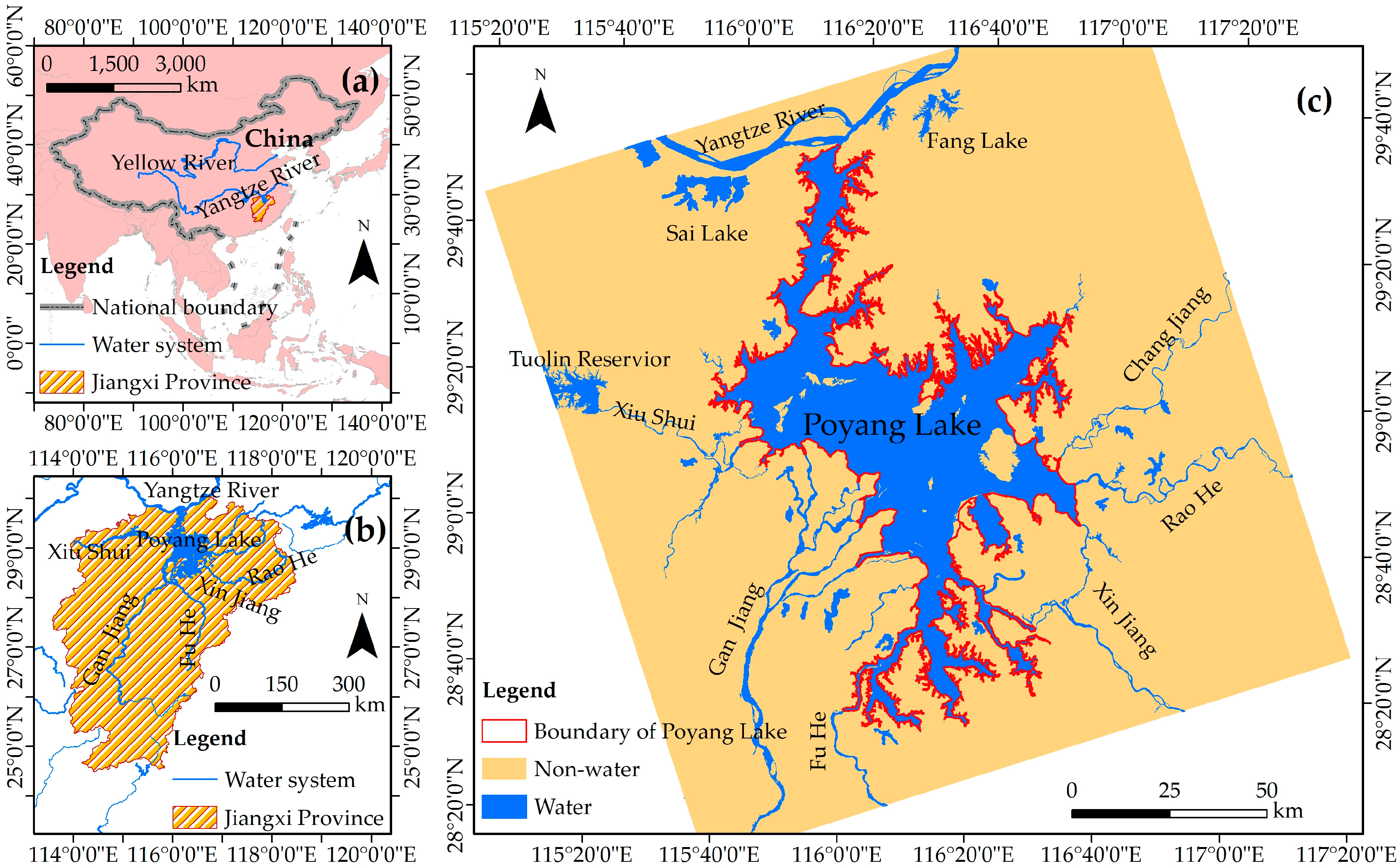
Poyang Lake, the largest freshwater lake in China, was selected as the study area. Poyang Lake is located in the northern Jiangxi Province (29°05′–29°17′N and 115°54′–116°08′E, southeastern China) and outflows into the Yangtze River at Hukou. The average water surface area of Poyang Lake is more than 2500 km
2 during the wet season [
6]. The lake is the primary component of the Poyang Lake wetland and has been included in the first set of the Ramsar Convention List of Wetlands of International Importance [
7]. The Poyang Lake region experiences a subtropical monsoon climate that is characterized by a rainy season (April to September) and a dry season (October to March) [
6]. The annual average temperature is 25 °C, and the annual average accumulative precipitation is approximately 1600 mm [
31]. The main water sources into the Poyang Lake are local precipitation and rivers (including the Xiushui, Ganjiang, Fuhe, Xinjiang, and Raohe rivers,
Figure 1) [
6].
Numerous small water bodies in the periphery have been disconnected from the large lake system because more than 500 levees have been built in Poyang Lake to protect approximately 5082 km
2 of farmland and settlements [
32,
33]. In addition, the boundary of the water surface of Poyang Lake is unstable and needs to be defined. The outline of the maximum water surface areas (on 17 July 2016) was defined as being approximately 4105 km
2 based on a previous study (
Figure 1) [
6].
Another minor study area is Taihu Lake, which is located in Jiangsu Province, China (30°56′–31°33′N and 119°52′–120°36′E) and is one of China’s five major freshwater lakes. This area was used to examine the results of the SWI-fitted equation and to examine the classification accuracy of S1A.
3. Materials and Methodology
3.1. Datasets and Preprocessing
Sentinel-1 is a polar orbiting two-satellite constellation (S1A and -B) that was launched by the European Space Agency (ESA) [
34]. S1A and -B, the next generation of C-band (center frequency 5.405 GHz) radar missions, were launched on 3 April 2014 and 25 April 2016, respectively, from Europe’s Spaceport in French Guiana. The revisit time of a single satellite is 12 days [
25], whereas the two-satellite constellation provides a revisit time of 6 days [
35]. The S1A utilized in the present study is a SAR standard L1 product, and belongs to the Interferometric Wide-swath mode (IW) with dual-polarization (VV/VH) [
26]. This data product has a wide coverage of 250 km with medium resolutions of 5 m and 20 m in range and azimuth directions, respectively, with an equivalent number of looks of five, and imagery pixel spacing of 10 m in ground geometry [
25]. For detailed descriptions regarding S1A, refer to reference [
25].
In the present study, 71 S1A scenes from 41 observations by Sentinel-1A satellite were selected from 24 May 2015 to 14 November 2016. Preprocessing of S1A imagery was performed with SNAP software provided by ESA (
https://sentinel.esa.int/web/sentinel/toolboxes/sentinel-1). The workflow included five steps. First, S1A images were allocated orbit files. Second, S1A images were radiometrically calibrated to output radar backscatter bands (
σ°). Third, radar backscatter bands were orthorectified using the Range Doppler Terrain Correction algorithm with SRTM DEM and spatial resolution of 1 s. Fourth, the backscattering coefficient (in dB) was acquired from the orthorectified radar backscatter band by the equation 10 × log
10 (
σ°) [
36]. Fifth, a median filter with window size of 5 × 5 pixel was utilized to remove speckle noises [
23,
37,
38].
A Landsat-8 satellite equipped with two sensor payloads (OLI and Thermal Infrared Sensor) was launched on 11 February 2013. In the present study, one OLI scene (acquired on 27 September 2016) was selected as the training data and applied for building the regression equation, and two OLI scenes (acquired on 9 September 2015 and 2 February 2016) were selected as testing data and applied to assess the classification accuracy of S1A. Eight OLI scenes (acquired on: 9 September 2015; 11 October 2015; 30 December 2015; 16 February 2016; 3 March 2016; 23 June 2016; 25 July 2016; and 27 September 2016) were used to extract the water surface areas of Poyang Lake and were compared with the water surface areas of Poyang Lake extracted from S1A from 24 May 2015 to 14 November 2016. Preprocessing work included atmospheric correction using the Fast Line-of-sight Atmospheric Analysis of Spectral Hypercube module, geometric correction, and data clipping based on the operational boundary of Poyang Lake. At the end, all images (S1A and OLI) were re-projected to an Asia North Albers Equivalent Conical Projection with the first standard parallel 25°N, the second standard parallel 47°N, and the central meridian 105°E.
3.2. Sentinel-1A Water Index
Water bodies create smooth and homogenous surfaces and, thereby, the return of radar pulses will be weak and the radar imagery over the area will be black or very dark in contrast with the surrounding non-water areas that produce a stronger return and brighter color [
39]. Optical water indexes, such as MNDWI, have the opposite characteristics. In MNDWI imagery, water bodies appear as brighter colors and non-water areas appear as darker colors. Thus, there is a negative correlation between S1A imagery and MNDWI imagery. The S1A water index (SWI) was built based on the linear regression equation between S1A (including VH and VV polarization) and MNDWI. Simultaneously, SWI has a characteristic similar to MNDWI computed from OLI based on the flowing equation [
30]:
where
represents the reflectance of the green band (B3 of OLI) and
represents the reflectance of the shortwave infrared band (B6 of OLI).
To match S1A pixels with MNDWI imagery pixels, the spatial resolution of S1A was resampled to 30 m (because the spatial resolution of MNDWI imagery is 30 m) using the nearest-neighbor method. Then, the MNDWI imagery and S1A (with spatial resolution of 30 m) were stacked using the stacking layer function in ENVI (version 4.8) software. Thus, a pixel on the stacked imagery had three attributes (e.g., VH (the abbreviation for the backscattering coefficient in VH polarization and VV has the same meaning), VV, and MNDWI values) and then a regression analysis was performed.
A total of 44,284 pairs of data were selected evenly and randomly from the stacked imagery to build the SWI. OLI and S1A were acquired on the same day (27 September 2016), which helped reduce the error from changes in water surface areas for different imaging dates when the SWI was built. These data cover the water body, grassland, forestland, farmland, bare land, and built-up land, with 42.31% being the water body. MNDWI and S1A were defined as dependent variables and independent variables, respectively. The SWI was built using the stepwise regression analysis method based on MNDWI, and six independent variables (VH, VV, VH × VV, VH2, VV2, and VH − VV) were derived from S1A.
3.3. Index Assessment
Several parameters including the root mean square error (RMSE), mean absolute error (MAE), root mean absolute percentage error (RMAPE), and R
2 were used to assess the SWI. These indexes are regularly employed in model evaluation studies and their expressions are as follows [
40,
41,
42]:
where
n is the total number of samples;
represents the observation value;
represents the estimated value;
represents the average observation value; and
represents the average estimated value. When RMSE, MAE, and RMAPE are low and
R2 is high, then the best-fit equation is achieved.
To examine the applicability of the SWI-fitted equation in different periods and regions, 190 and 225 pairs of testing data (SWI and MNDWI, respectively) were selected randomly from S1A and OLI images acquired on 2 February 2016, in the Taihu Lake region, China, and 9 September 2015, in the Poyang Lake region, respectively, to examine the fitted SWI using the indexes mentioned above.
3.4. Extraction of the Water Area
The water area extracted from OLI was regarded as the ground-truth water area and was extracted using the threshold method. If the MNDWI value of a pixel is more than 0 and the normalized difference vegetation index (
NDVI) value is less than 0.15, it is classified as water. The NDVI was computed from OLI based on the flowing equation:
where
represents the reflectance of the near-infrared band (B5 of OLI) and
represents the reflectance of the red band (B4 of OLI).
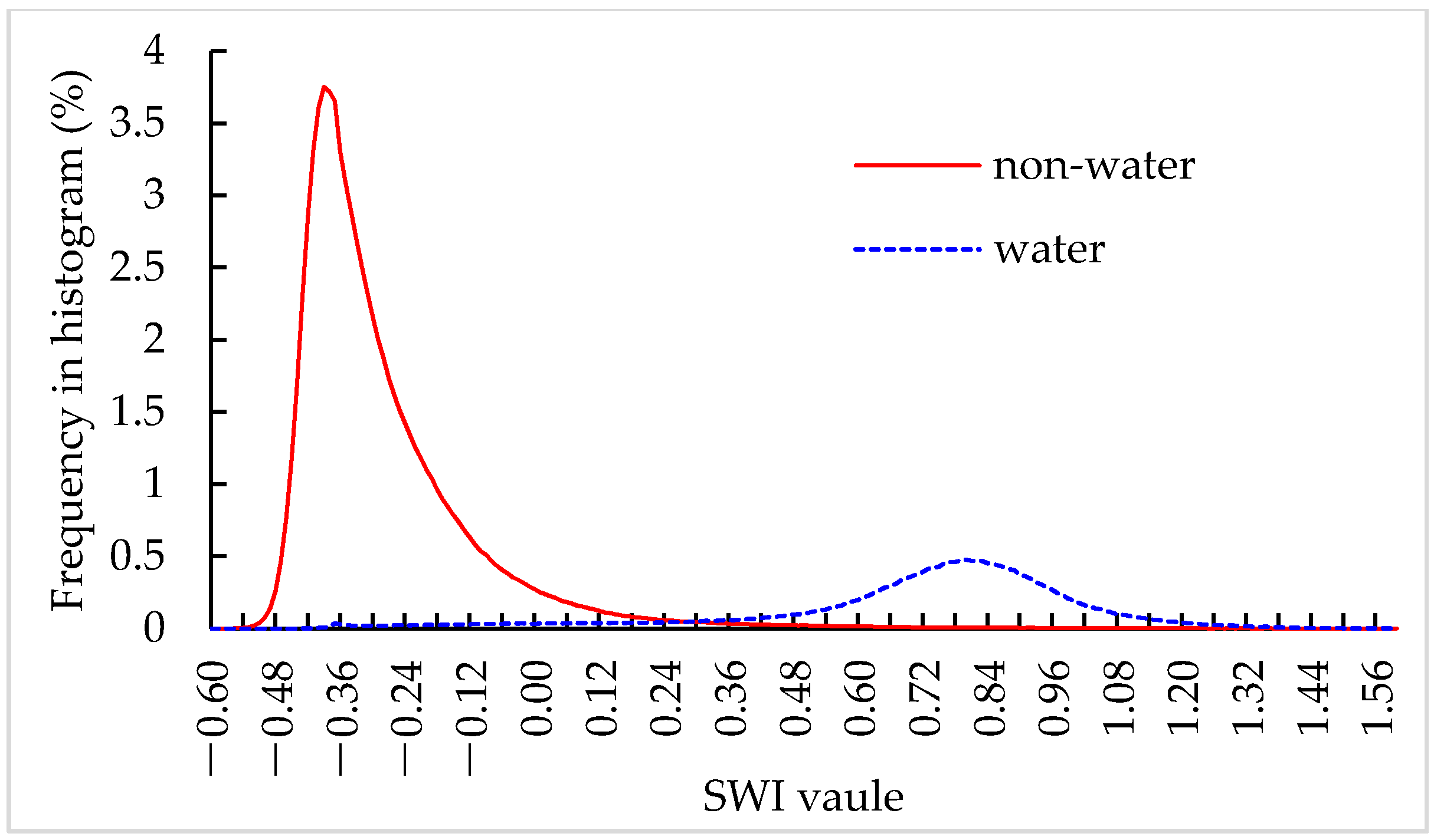
The histogram frequency of the SWI imagery (on 27 September 2016) based on the ground-truth water and non-water is plotted in
Figure 2 to facilitate visualization.
Figure 2 demonstrates that the majority of the SWI water values are more than 0.40 and the majority of the SWI non-water values are less than 0.18 through visual judgment. However, an appropriate and unique threshold ranging from 0.18 to 0.40 needed to be determined by calculating the positive and negative errors. The threshold is regarded as appropriate when the classification errors of water and non-water are approximate and the overall accuracy derived from the confusion matrix is optimal (the sum of positive and negative errors comes to the minimal value). The result showed that the sum is minimal (0.02%) when the threshold is 0.20. In the present study, the water information of Poyang Lake was extracted using the threshold method from 24 May 2015 to 14 November 2016.
3.5. Evaluation of Quantity Accuracy
The water area extracted from OLI was regarded as the ground-truth water area [
24] to examine the classification accuracy of S1A in three steps. First, the spatial resolution of S1A was resized to 30 m using the nearest-neighbor method to match the spatial resolution of OLI. Then, three periods of ground-truth water areas from OLI (two OLI scenes acquired on 9 September 2015 and 27 September 2016 in Poyang Lake region, and one OLI scene acquired on 2 February 2016 in the Taihu Lake region) were selected to assess the accuracy of the SWI category during different periods and in different regions using the confusion matrix method. Finally, quantity accuracy was computed with the following equation:
where
represents the quantity accuracy;
Aextracted represents the water surface area extracted from SWI imagery; and
Atruth represents the ground-truth water area extracted from the OLI bands.
3.6. Dynamic Change Analysis Method
To understand the characteristics and influences of the water changes in Poyang Lake, the submergence ratio was computed as the following equation for each pixel:
where
δratio represents the submergence ratio;
n represents the number of inundations observed by S1A; and
N represents the total observations times of S1A (i.e., 41 in this study). The submergence ratio approximates the probability of being submerged for each pixel.
Poyang Lake is composed of a number of lakes with different areas. Lakes were grouped to facilitate the statistical change detection analyses into the following classes: 0.1–1.0 km2, >1.0–10 km2, and >10–100 km2. The change in the number of lakes with different areas was analyzed to explain the dynamic change in the Poyang Lake water surface areas in this study.
3.7. Extraction of Water Surface Areas from SWI, VH, and VV Images Using Different Methods
In order to prove that the SWI image is better than the original image of S1A (including the VH image and VV image) to extract water, four classification methods were used, i.e., the threshold classification method (TCM), IsoData unsupervised classification (IUC), Minimum Distance Classification (MDC), and Support Vector Machine (SVM). The test zone was a rectangle with an area of 110 km × 70 km location in the Poyang Lake region.
Similar to
Figure 2 and its theory, the threshold values were confirmed as −23 dB and −17 dB based on VH and VV imagery, respectively. For a single band, a pixel was classified as water if its value was less than −23 dB in VH imagery or −17 dB in VV imagery, respectively. For double bands, a pixel was classified as water if its value was less than −23 dB in VH imagery and −17 dB in VV imagery.
IUC is barely affected by subjectivity [
43,
44] and the classification results utilizing IUC demonstrate the ability of the imagery to distinguish between water and non-water areas. Water was extracted from the original image of S1A and SWI image using the same default parameters of IUC model in ENVI software.
MDC and SVM are supervised classification methods that are used in many studies [
23,
45,
46]. The resamples (1937 pixels) used in MDC and SVM were randomly selected based on the ground-truth water extracted from OLI. The resamples are the same when extracting water from the original image and the SWI image using MDC and SVM.
3.8. Extraction of Water Surface Areas from MODIS Data
To understand the ability to identify the details of the water, the classification accuracy of water extracted from the MODIS image was evaluated based on the ground-truth water extracted from OLI. The MODIS image was acquired on 27 September 2016. The green band (B4 of MODIS, center wavelength 555 nm) and the shortwave infrared band (B6 of MODIS, center wavelength 1640 nm) were used to compute the MNDWI according to Equation (1). The red band (B1 of MODIS, center wavelength 645 nm) and the near-infrared band (B2 of MODIS, center wavelength 860 nm) were used to compute the NDVI according to Equation (6). If the MNDWI value of a pixel is more than 0 and the NDVI value of a pixel is less than 0.15, it is classified as water. Thus, the water image form MODIS was obtained. Then, the water image form MODIS was resized to 30 m using the nearest-neighbor method when building the accuracy assessment confusion matrix.
4. Results
4.1. The SWI-Fitted Equation
VV, VH × VV, VV
2, and VH
2 were selected with the stepwise regression analysis method. The SWI fitted equation was as follows:
where
and
represent the backscattering coefficient in VH polarization and VV polarization, respectively.
The R2 of the SWI fitted equation was 0.83, the RMSE was 0.23, the F-value was 31,874, and the p-value was less than 0.01. Therefore, the SWI fitted equation was statistically significant.
Table 1 shows the examination results of the SWI fitted equation in different periods and regions. The data in
Table 1 show that the SWI-fitted equation was statistically significant.
4.2. Water Area Extraction Using SWI
The best classification results were obtained using the threshold of 0.2 to distinguish water and non-water from the SWI images.
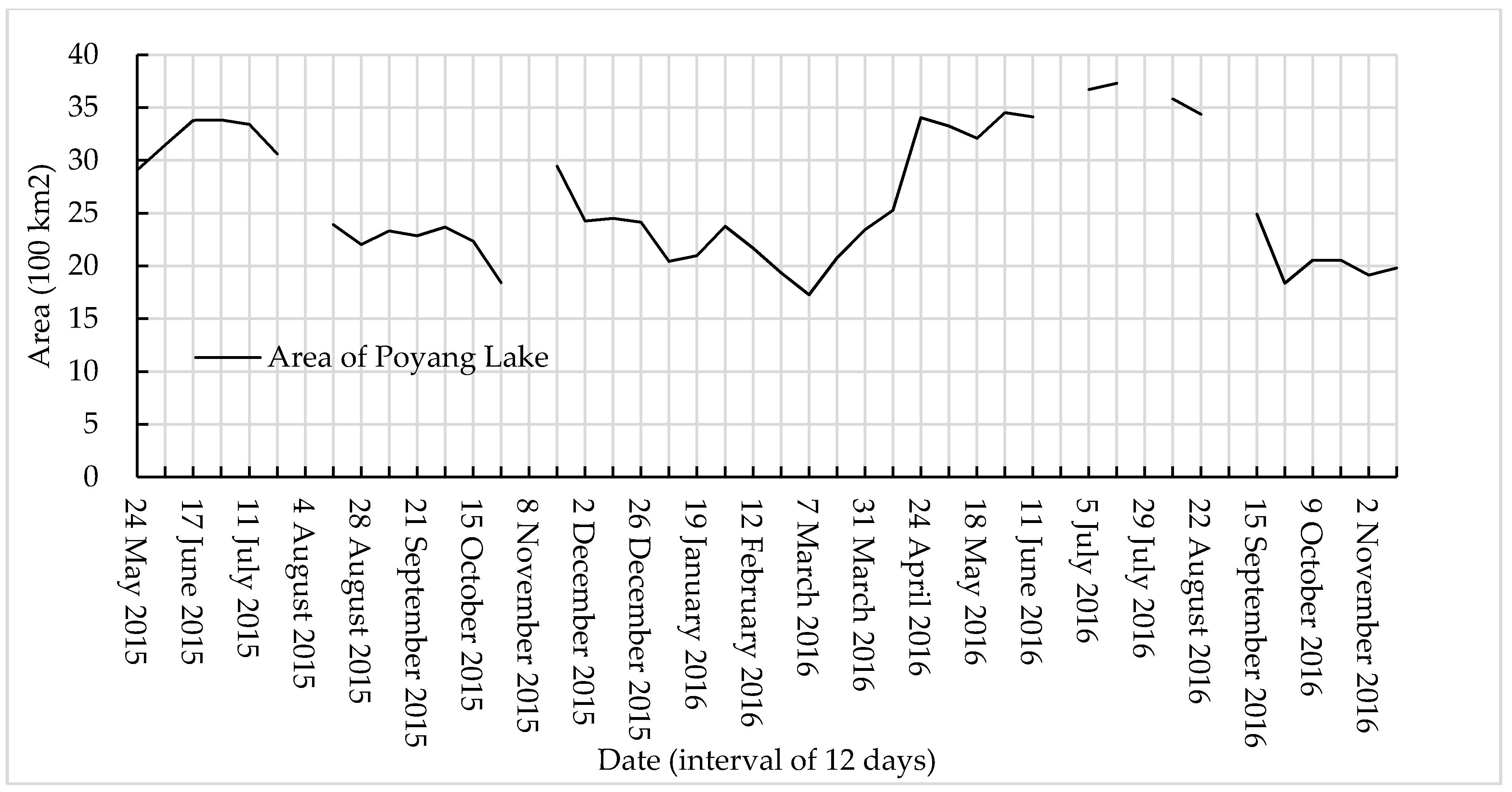
Figure 3 and
Figure 4 show the extracted water surface areas of Poyang Lake from 24 May 2015 to 14 November 2016, with an interval of 12 days. The average, maximum, and minimum areas of Poyang Lake were 2638.36 km
2, 3729.19 km
2 (on 17 July 2016), and 1726.73 km
2 (on 7 March 2016), respectively.
To better understand the dynamic changes of the water surface areas of Poyang Lake, the changed area and the variation rate of the water surface areas in 12-day intervals were analyzed. During the period of analysis, there were 22 changes of more than 100 km2. The maximum changed area was 875.57 km2 with a variation rate of 35% from 12 April to 24 April 2016. The average changed area was 197.58 km2. The variation rate in each 12-day interval showed that there were 11 changes of >10%. The average variation rate was 8.2%. The water surface areas of Poyang Lake had several significant changes within a 12-day window over the course of the study period.
4.3. Accuracy Evolution
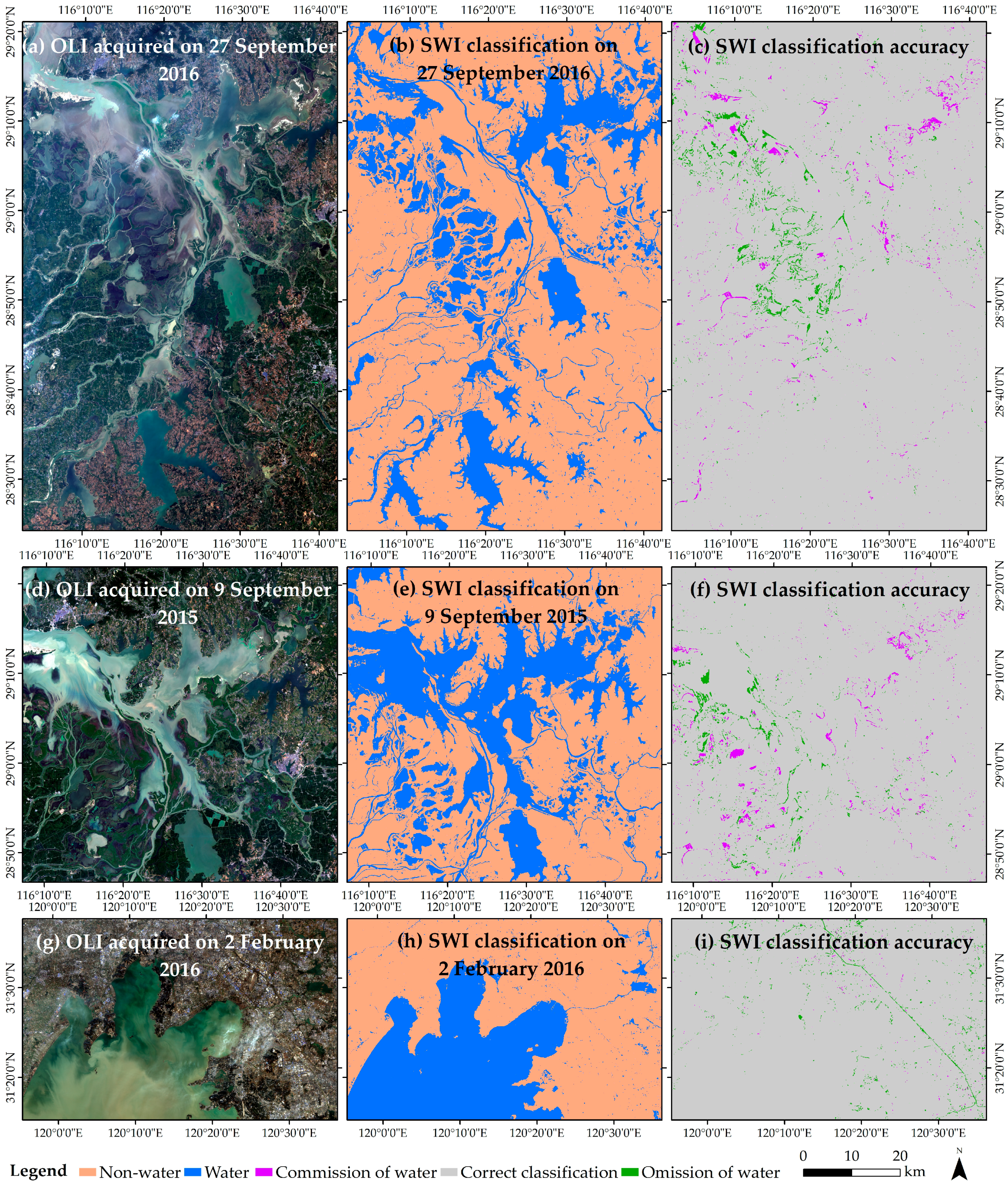
The classification accuracy of SWI is presented in
Table 2 and plotted in
Figure 5 to facilitate visualization. In the Poyang Lake region, the overall accuracy was more than 96%. On 27 September 2016, the producer’s accuracy and user’s accuracy of water were 91.51% and 92.58%, respectively. On 9 September 2015, the producer’s accuracy and user’s accuracy of water were 94.18% and 93.41%, respectively. The approximation between producer’s accuracy and user’s accuracy leads to higher quantity accuracy than it does overall accuracy because the rates of omission and commission counteract. The quantity accuracy of water was 99.18% and 98.84% on 9 September 2015 and 27 September 2016, respectively. The accuracy was also superior in the Taihu Lake region. Therefore, the SWI threshold classification method could be applied to different regions during different periods with high and reliable accuracy.
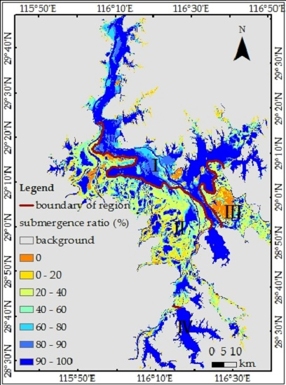
4.4. Submergence Ratio Analysis
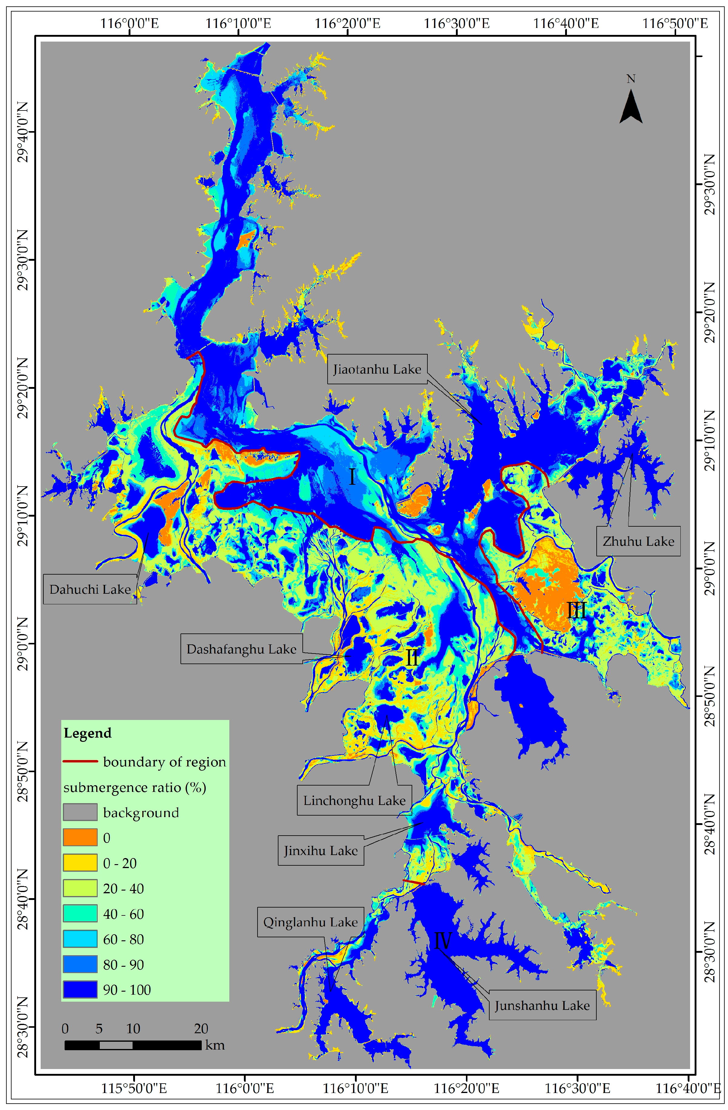
The submergence ratio can document the spatiotemporal dynamic change of the water surface areas of Poyang Lake and is plotted in
Figure 6. The area that was submerged 100% of the time was 1307.41 km
2, or 31.85% of the entirety of Poyang Lake; 876.07 km
2, or 29.04% was submerged between 80% and 100%; and 1605.61 km
2, or 39.11%, was submerged for less than 60% of the study period.
The change characteristics of Poyang Lake had obvious regional differences. To expediently describe the change characteristics in different regions, Poyang Lake was roughly divided into four regions based on submergence ratios (
Figure 6, Regions I–IV). As a whole, the submergence ratio was more than 90% for the majority of Regions I and IV, less than 40% for the majority of Region III, and Region II had a complex submergence ratio. In Region II, there were many isolated lakes whose submergence ratios were more than 90% and had an area of 430.36 km
2 (27% of the total area in Region II), and there were many districts whose submergence ratios were less than 40% with an area of 717.88 km
2 (44% of the total area in Region II). During this study period, the variation rate in the changed area of Region II was the greatest among the four regions. The maximum variation rate was 80% between 12 April and 24 April 2016, with an average variation rate of 13% in Region II.
4.5. The Number of Lake with Different Area
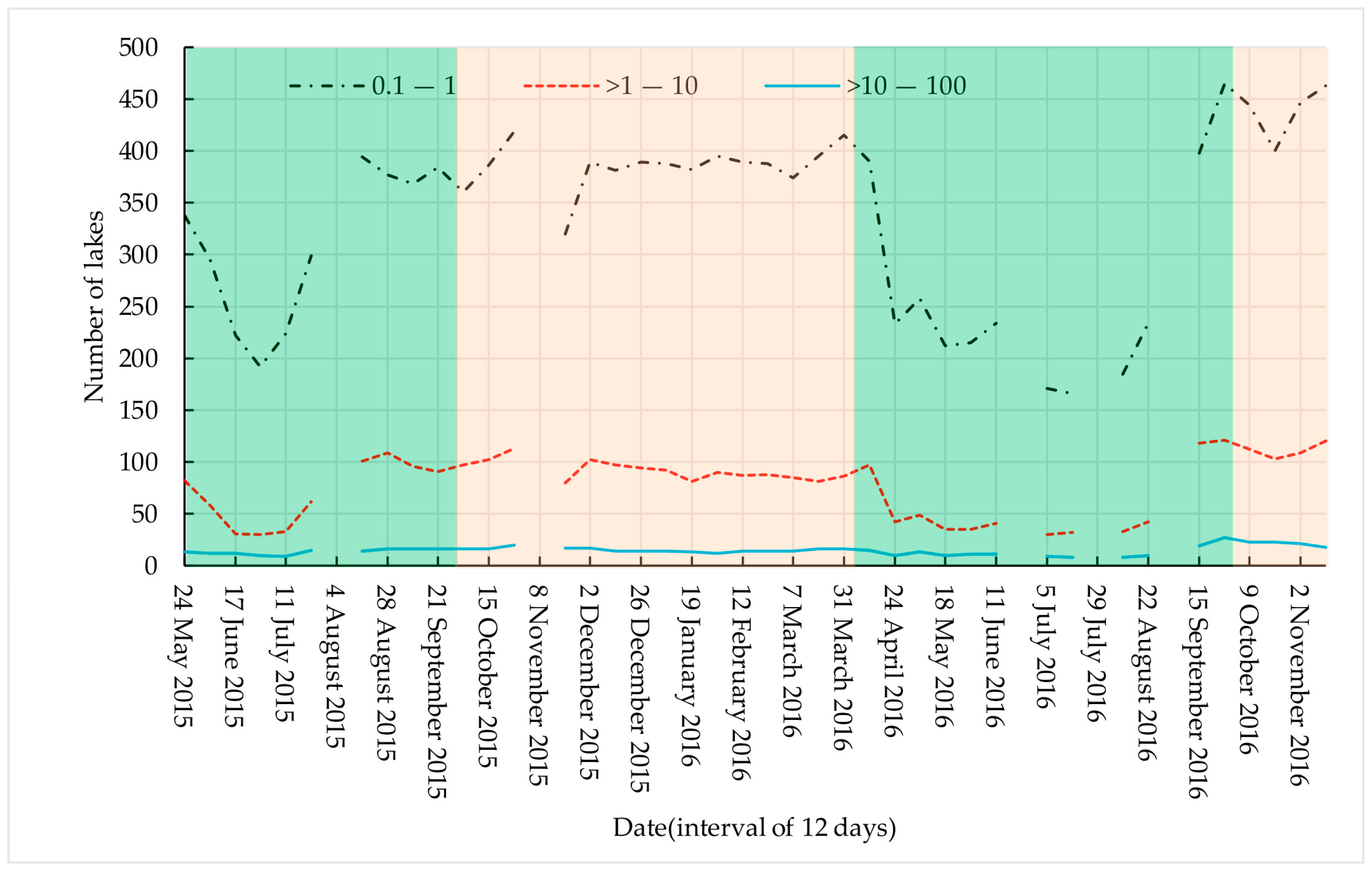
Poyang Lake is composed of a number of lakes (
Figure 7). The number of lakes with an area of 0.1–1 km
2 ranged from 166 to 465 (average 336) in this study. The number of lakes with an area of >1–10 km
2 ranged from 30 to 121 (average 78). The number of lakes with an area of >10–100 km
2 ranged from 8 to 27 (average 15).
During the rainy season, from April to September, the water surface areas can expand to >3000 km2 and form several big lakes, and during the dry season, from October to March, the water surface areas can shrink to <2000 km2 and a number of small and isolated lakes are then segregated from the big lakes. The number of lakes of 0.1–1 km2 drastically fluctuated. During the dry season, the average, maximum, and minimum number of lakes was approximately 396, 465, and 320, respectively. During the rainy season, the average, maximum, and minimum number of lakes was approximately 232, 338, and 166, respectively. The change in the number of lakes of 0.1–1 km2 in 12-day intervals was analyzed. The maximum change in number was 157 in the 12-day interval from April 12 to April 24, 2016. The average change in number was 31, which means that 31 lakes of 0.1–1 km2 disappeared or appeared within 12-day intervals.
4.6. Comparison of Water Area Extracted Using Different Method and Different Data
Table 3 shows that the quantity accuracy and overall accuracy of water extracted from SWI imagery was higher than that of the original imagery of S1A using the four methods based on the ground-truth water area that was extracted from OLI acquired on 27 September 2016.
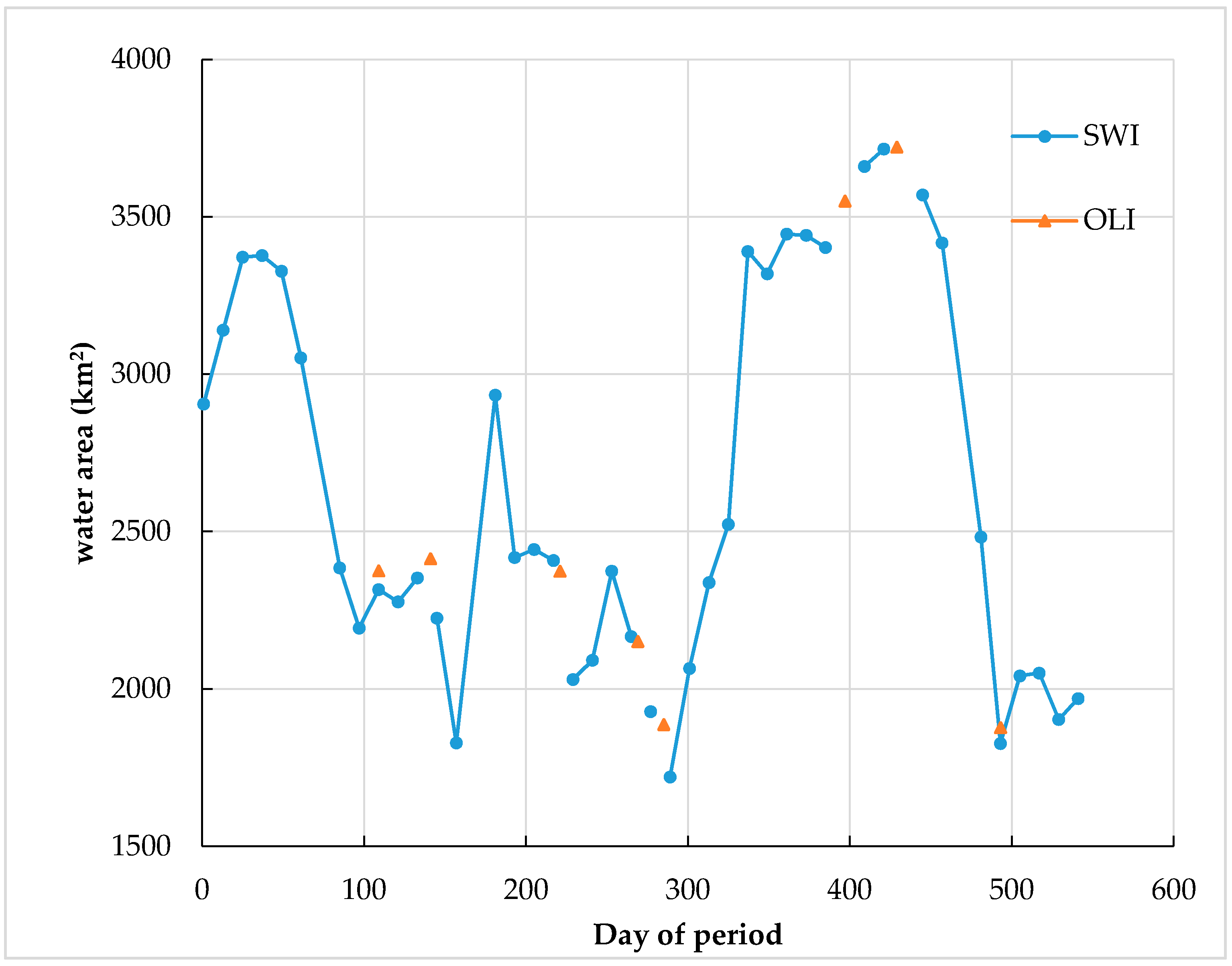
The water surface areas of Poyang Lake extracted from OLI and SWI are plotted in
Figure 8. There were only eight OLI scenes that were cloud-free from 24 May 2015 to 14 November 2016 (
Figure 8), and many variation characteristics of the water were not detected by OLI compared with the results from the SWI images.
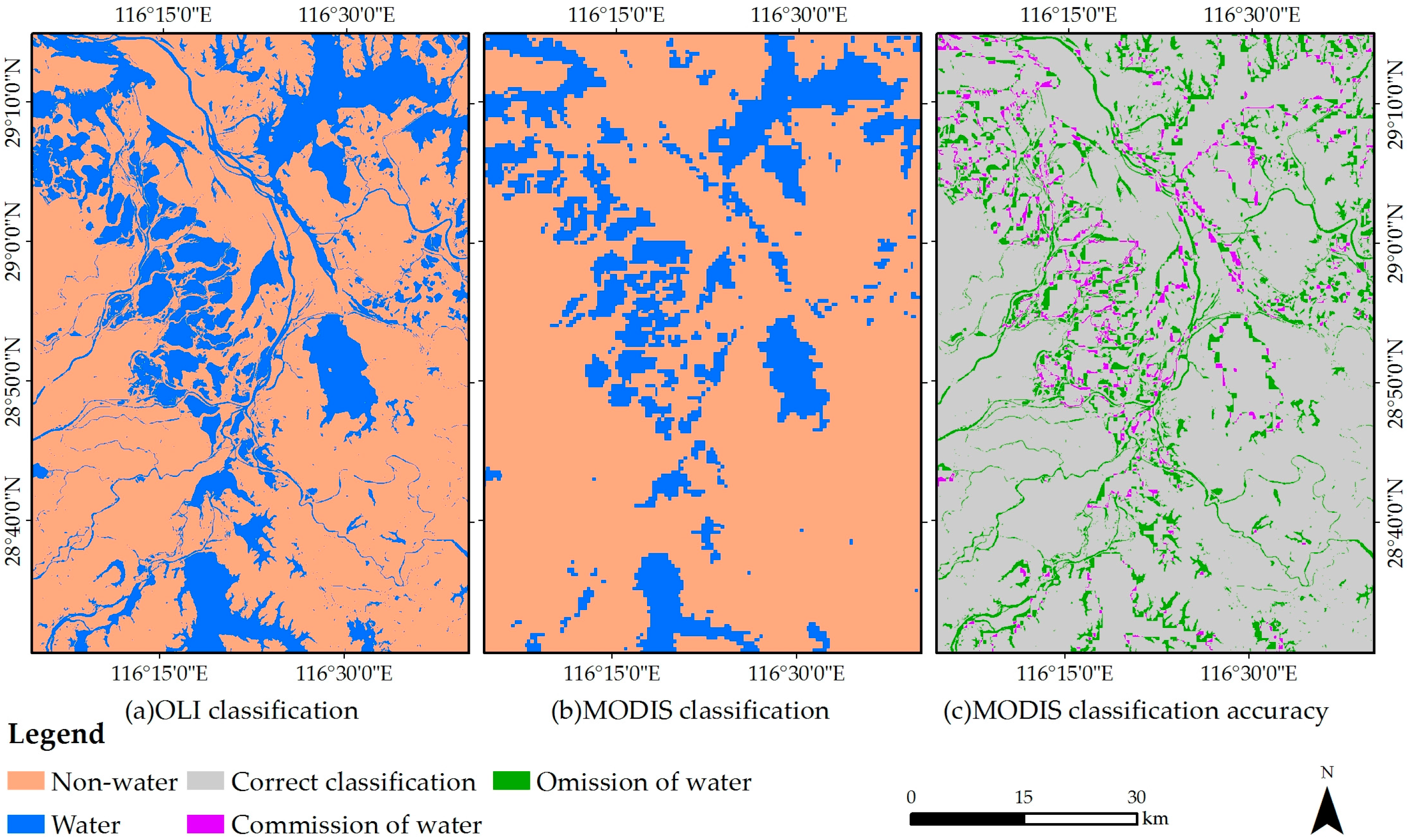
Water extracted from MODIS on 27 September 2016 is shown in
Figure 9b. The classification accuracy was assessed based on the ground-truth water area from OLI. The quantity accuracy was 67.56% (omission 537 km
2). The overall accuracy was 88.96% (kappa coefficient 0.64) and the producer’s accuracy was only 58.71%, which indicates that 41.29% of the water was omitted (see
Figure 9c). The quantity accuracy and overall accuracy from the SWI image were 31.28% and 7.56% higher, respectively, than that from the MODIS image.
5. Discussion
The edges of the water body are the main zones where incorrect classification occurred since these environments are very complex (e.g., there were widely distributed shallows, sand, and plankton) in the present study (
Figure 5). The zones of the commission of water mainly appeared as a light-green and bright white color in OLI (
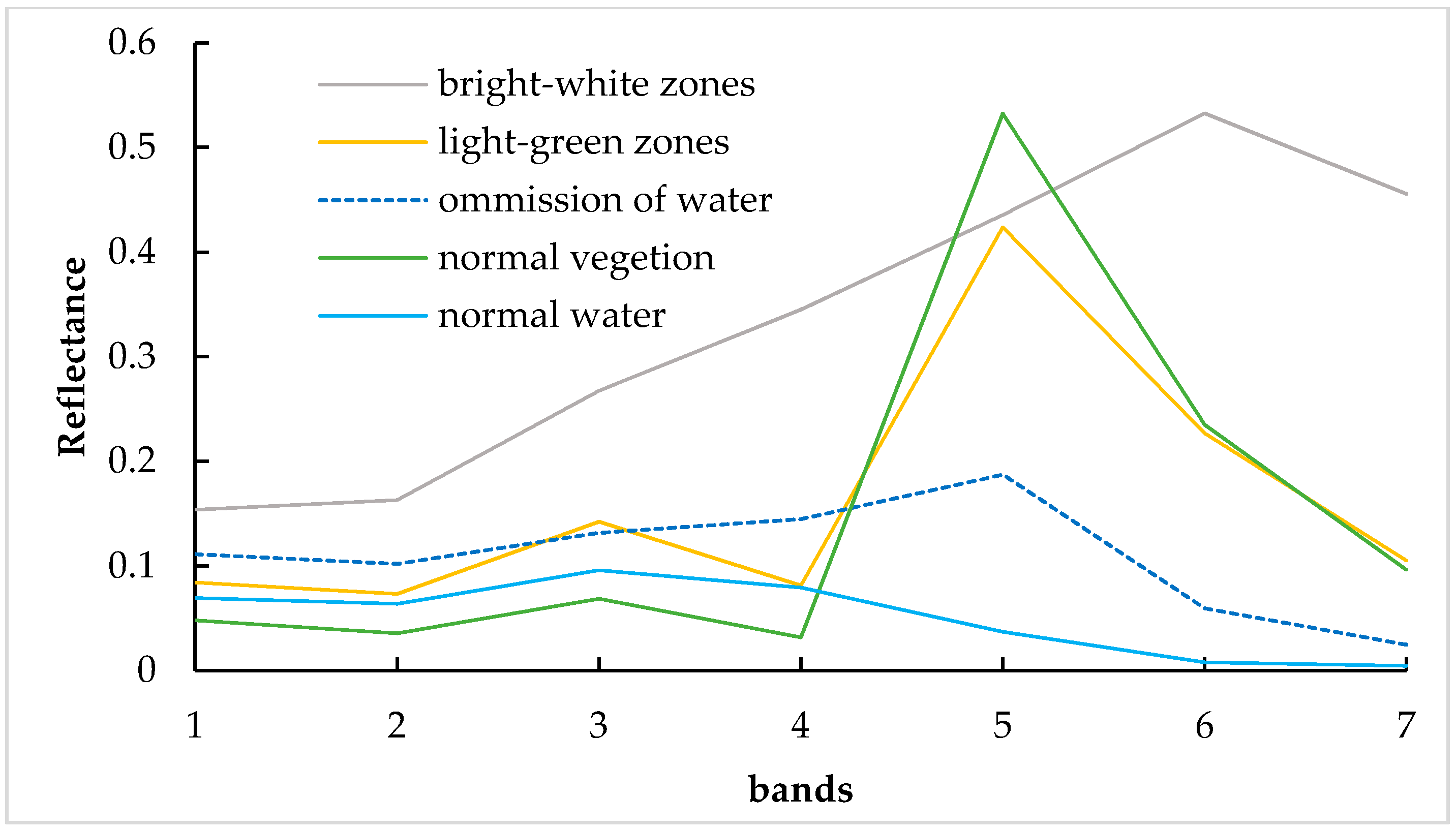
Figure 10a). There were sparse emergent aquatic plants or plankton in the light-green zones, whose spectral characteristics were similar to the vegetation (
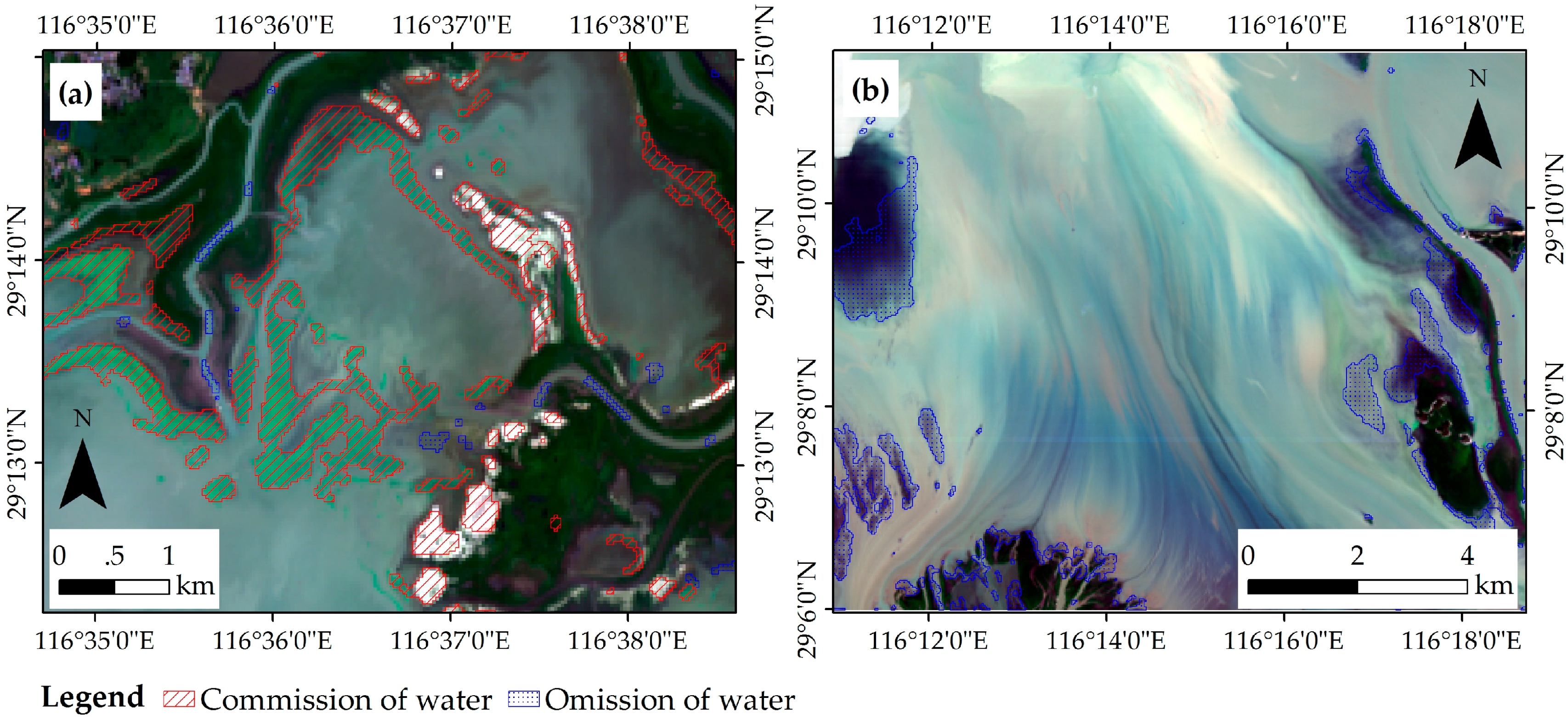
Figure 11). Thus, these zones might be categorized as vegetation in the OLI images. However, in these zones, the main return of the radar pulse came from the water due to the low density of vegetation. Thus, these zones were categorized as water in the SWI images, which should be regarded as correct. The bright white zones were sand with high water content and low surface roughness; therefore, these bright white zones were wrongly categorized as water in the SWI image.
We cannot determine whether the omission water (
Figure 10b) was part of the water body because its spectral characteristics were different from those of normal water (
Figure 11). However, they were categorized as water in the MNDWI image. Therefore, further study is required to investigate this.
Compared with the original images of S1A, SWI images have the ability to enhance the difference between water and non-water. Furthermore, high speed, efficiency, and classification accuracy are regarded as being advantages of the SWI threshold classification method for extracting water from SWI imagery, as shown in
Table 3.
Table 3 also shows that the area of water can be extracted with the highest QA of 99.57% using the SVM method with SWI data. However, when compared to the similarly performing TCM method (QA: 98.84%, see
Table 3), it is more time consuming to analyze inundation extent using SVM.
Compared to the OLI and MODIS images, SWI images have high effective spatiotemporal resolution. The revisit time of OLI is 16 days, and the frequency of cloudy or rainy weather is very high in the south of China. Therefore, there is a lack of useful OLI data when detecting the dynamic changes in Poyang Lake (
Figure 8).
Although MODIS has a revisit time of one day, its spatial resolution is too coarse to identify the details of the water and small water bodies. Poyang Lake is composed of a number of lakes with areas of less than 1 km
2 that are easily omitted from MODIS. The annual water surface area of Poyang Lake extracted from MODIS ranged from 700 km
2 to 2700 km
2 during 2000 to 2010 [
6]; however, the water surface area ranged from 1700 km
2 to 3700 km
2 in the present study. Additionally, the quantity accuracy from MODIS was 67.56%, and meaning that water surface area of 537 km
2 wasn’t detected by MODIS in sub-region in the
Figure 9. It may be possible to improve the quantity accuracy by other advanced methods, although we still believe that MODIS cannot precisely identify details of the water and small water bodies, especially in areas where water changes are severe.
6. Conclusions
In the present study, a new water index (SWI) was constructed based on S1A and OLI-MNDWI using the multiple stepwise regression analysis method. The best classification results were obtained using the threshold of 0.2 to distinguish water and non-water from the SWI images. The advantages of extracting water using the SWI are that it is quick and more efficient than the other Machine Learning methods. In addition, the SWI threshold classification method can be applied to different regions during different periods with high quantity accuracy (approximately 99%) and overall accuracy (approximately 97%).
A total of 41 days of water surface areas for Poyang Lake were extracted from 24 May 2015 to 14 November 2016, with an interval of 12 days. The average area of Poyang Lake was 2638.36 km2 during the study period. The maximum and minimum areas were 3729.19 km2 (on 17 July 2016) and 1726.73 km2 (on 7 March 2016), respectively. The results showed that changes in water surface areas were dramatic within periods of 12 days. The maximum and average changed areas were 875.57 km2 (with a change rate of 35% from 12 April to 24 April 2016) and 197.58 km2 (with a change rate of 8.2%) in 12 days, respectively. Moreover, the change in the mid-western region of Poyang Lake was more marked, with a maximum change rate of 80% between 12 April and 24 April 2016, and an average change rate of 13%.
Poyang Lake is composed of a number of lakes, with the number drastically fluctuating with the changes in water surface area. The number of lakes with areas of 0.1–1 km2, >1–10 km2, and >10–100 km2 ranged from 166 to 465, from 30 to 121, and from 8 to 27, respectively, in the present study.
These results provide scientific guidance and baseline data for high-frequency monitoring of the ecological environment and wetland management in Poyang Lake.
Acknowledgments
This study was supported by the National Natural Science Foundation of China (41301390 and U1404401) and the Youth Innovation Promotion Association CAS (2017089).
Author Contributions
Haifeng Tian, Mingquan Wu, and Zheng Niu conceived and designed the methodology; Haifeng Tian and Wang Li performed the methodology; Ni Huang, Guodong Li, and Xiang Li analyzed the data; and Haifeng Tian wrote the paper.
Conflicts of Interest
The authors declare no conflict of interest.
References
- Ma, R.H.; Duan, H.T.; Hu, C.M.; Feng, X.Z.; Li, A.N.; Ju, W.M.; Jiang, J.H.; Yang, G.S. A half-century of changes in China’s lakes: Global warming or human influence? Geophys. Res. Lett. 2010, 37, 6. [Google Scholar] [CrossRef]
- Tao, S.L.; Fang, J.Y.; Zhao, X.; Zhao, S.Q.; Shen, H.H.; Hu, H.F.; Tang, Z.Y.; Wang, Z.H.; Guo, Q.H. Rapid loss of lakes on the mongolian plateau. Proc. Natl. Acad. Sci. USA 2015, 112, 2281–2286. [Google Scholar] [CrossRef] [PubMed]
- Hui, J.; Yao, L. Analysis and inversion of the nutritional status of China’s Poyang Lake using MODIS data. J. Indian Soc. Remote Sens. 2016, 44, 837–842. [Google Scholar] [CrossRef]
- Yang, P.; Liu, X.H.; Xu, B. Spatiotemporal pattern of bird habitats in the Poyang Lake based on landsat images. Environ. Earth Sci. 2016, 75, 8. [Google Scholar] [CrossRef]
- Tang, X.G.; Li, H.P.; Xu, X.B.; Yang, G.S.; Liu, G.H.; Li, X.Y.; Chen, D.Q. Changing land use and its impact on the habitat suitability for wintering anseriformes in China’s Poyang Lake region. Sci. Total Environ. 2016, 557, 296–306. [Google Scholar] [CrossRef] [PubMed]
- Feng, L.; Hu, C.M.; Chen, X.L.; Cai, X.B.; Tian, L.Q.; Gan, W.X. Assessment of inundation changes of Poyang Lake using MODIS observations between 2000 and 2010. Remote Sens. Environ. 2012, 121, 80–92. [Google Scholar] [CrossRef]
- Wu, G.P.; Liu, Y.B. Capturing variations in inundation with satellite remote sensing in a morphologically complex, large lake. J. Hydrol. 2015, 523, 14–23. [Google Scholar] [CrossRef]
- Yu, G.; Shen, H.D. Lake water changes in response to climate change in northern China: Simulations and uncertainty analysis. Quat. Int. 2010, 212, 44–56. [Google Scholar] [CrossRef]
- Bryant, M.D. Global climate change and potential effects on pacific salmonids in freshwater ecosystems of southeast alaska. Clim. Chang. 2009, 95, 169–193. [Google Scholar] [CrossRef]
- Dronova, I.; Gong, P.; Wang, L. Object-based analysis and change detection of major wetland cover types and their classification uncertainty during the low water period at Poyang Lake, China. Remote Sens. Environ. 2011, 115, 3220–3236. [Google Scholar] [CrossRef]
- Sica, Y.V.; Quintana, R.D.; Radeloff, V.C.; Gavier-Pizarro, G.I. Wetland loss due to land use change in the lower parana river delta, argentina. Sci. Total Environ. 2016, 568, 967–978. [Google Scholar] [CrossRef] [PubMed]
- Feng, L.; Han, X.; Hu, C.; Chen, X. Four decades of wetland changes of the largest freshwater lake in China: Possible linkage to the three gorges dam? Remote Sens. Environ. 2016, 176, 43–55. [Google Scholar] [CrossRef]
- Kutser, T.; Pierson, D.C.; Kallio, K.Y.; Reinart, A.; Sobek, S. Mapping lake cdom by satellite remote sensing. Remote Sens. Environ. 2005, 94, 535–540. [Google Scholar] [CrossRef]
- Kallio, K. Remote sensing monitors lakes. Trac Trends Anal. Chem. 2012, 34, 3–4. [Google Scholar]
- Giardino, C.; Bresciani, M.; Stroppiana, D.; Oggioni, A.; Morabito, G. Optical remote sensing of lakes: An overview on lake maggiore. J. Limnol. 2014, 73, 201–214. [Google Scholar] [CrossRef]
- Wright, R.; Pilger, E. Satellite observations reveal little inter-annual variability in the radiant flux from the mount erebus lava lake. J. Volcanol. Geotherm. Res. 2008, 177, 687–694. [Google Scholar] [CrossRef]
- Veettil, B.K.; Bianchini, N.; de Andrade, A.M.; Bremer, U.F.; Simoes, J.C.; de Souza, E. Glacier changes and related glacial lake expansion in the bhutan himalaya, 1990–2010. Reg. Environ. Chang. 2016, 16, 1267–1278. [Google Scholar] [CrossRef]
- Hereher, M.E. Environmental monitoring and change assessment of toshka lakes in southern egypt using remote sensing. Environ. Earth Sci. 2015, 73, 3623–3632. [Google Scholar] [CrossRef]
- Zhu, X.L.; Chen, J.; Gao, F.; Chen, X.H.; Masek, J.G. An enhanced spatial and temporal adaptive reflectance fusion model for complex heterogeneous regions. Remote Sens. Environ. 2010, 114, 2610–2623. [Google Scholar] [CrossRef]
- Wu, M.Q.; Wu, C.Y.; Huang, W.J.; Niu, Z.; Wang, C.Y.; Li, W.; Hao, P.Y. An improved high spatial and temporal data fusion approach for combining Landsat and MODIS data to generate daily synthetic Landsat imagery. Inf. Fusion 2016, 31, 14–25. [Google Scholar] [CrossRef]
- Gao, F.; Masek, J.; Schwaller, M.; Hall, F. On the blending of the Landsat and MODIS surface reflectance: Predicting daily Landsat surface reflectance. IEEE Trans. Geosci. Remote Sens. 2006, 44, 2207–2218. [Google Scholar]
- Wu, M.Q.; Niu, Z.; Wang, C.Y.; Wu, C.Y.; Wang, L. Use of MODIS and Landsat time series data to generate high-resolution temporal synthetic Landsat data using a spatial and temporal reflectance fusion model. J. Appl. Remote Sens. 2012, 6, 063507. [Google Scholar]
- Tian, H.; Wu, M.; Niu, Z.; Wang, C.; Zhao, X. Dryland crops recognition under complex planting structure based on radarsat-2 images. Trans. Chin. Soc. Agric. Eng. 2015, 31, 154–159. [Google Scholar]
- Long, S.; Fatoyinbo, T.E.; Policelli, F. Flood extent mapping for namibia using change detection and thresholding with SAR. Environ. Res. Lett. 2014, 9. [Google Scholar] [CrossRef]
- Torres, R.; Snoeij, P.; Geudtner, D.; Bibby, D.; Davidson, M.; Attema, E.; Potin, P.; Rommen, B.; Floury, N.; Brown, M.; et al. Gmes Sentinel-1 mission. Remote Sens. Environ. 2012, 120, 9–24. [Google Scholar] [CrossRef]
- Cazals, C.; Rapinel, S.; Frison, P.L.; Bonis, A.; Mercier, G.; Mallet, C.; Corgne, S.; Rudant, J.P. Mapping and characterization of hydrological dynamics in a coastal marsh using high temporal resolution Sentinel-1a images. Remote Sens. 2016, 8, 17. [Google Scholar] [CrossRef]
- Qiao, C.; Luo, J.C.; Sheng, Y.W.; Shen, Z.F.; Zhu, Z.W.; Ming, D.P. An adaptive water extraction method from remote sensing image based on NDWI. J. Indian Soc. Remote Sens. 2012, 40, 421–433. [Google Scholar] [CrossRef]
- Gu, Y.X.; Hunt, E.; Wardlow, B.; Basara, J.B.; Brown, J.F.; Verdin, J.P. Evaluation of MODIS NDVI and NDWI for vegetation drought monitoring using oklahoma mesonet soil moisture data. Geophys. Res. Lett. 2008, 35, 5. [Google Scholar] [CrossRef]
- Gao, B.C. NDWI-a normalized difference water index for remote sensing of vegetation liquid water from space. Remote Sens. Environ. 1996, 58, 257–266. [Google Scholar] [CrossRef]
- Xu, H.Q. Modification of normalised difference water index (NDWI) to enhance open water features in remotely sensed imagery. Int. J. Remote Sens. 2006, 27, 3025–3033. [Google Scholar] [CrossRef]
- Li, Y.; Zhang, Q.; Li, X.; Yao, J. Hydrolgical effects of Poyang Lake catchment in response to climate changes Resour. Environ. Yangtze Basin 2013, 22, 1339–1347. [Google Scholar]
- Qi, S.; Brown, D.G.; Tian, Q.; Jiang, L.; Zhao, T.; Bergen, K.A. Inundation extent and flood frequency mapping using Landsat imagery and digital elevation models. Gisci. Remote Sens. 2009, 46, 101–127. [Google Scholar] [CrossRef]
- Cai, X.; Gan, W.; Ji, W.; Zhao, X.; Wang, X.; Chen, X. Optimizing remote sensing-based level-area modeling of large lake wetlands: Case study of Poyang Lake. IEEE J. Sel. Top. Appl. Earth Obs. Remote Sens. 2015, 8, 471–479. [Google Scholar] [CrossRef]
- Plank, S. Rapid damage assessment by means of multi-temporal SAR-a comprehensive review and outlook to Sentinel-1. Remote Sens. 2014, 6, 4870–4906. [Google Scholar] [CrossRef]
- Jung, H.S.; Lu, Z.; Zhang, L. Feasibility of along-track displacement measurement from Sentinel-1 interferometric wide-swath mode. IEEE Trans. Geosci. Remote Sens. 2013, 51, 573–578. [Google Scholar] [CrossRef]
- Li, K.; Shao, Y.; Zhang, F. Rice information extraction using multi-polarization airborne synthetic aperture radar data. J. Zhejiang Univ. Agric. Life Sci. 2011, 37, 181–186. [Google Scholar]
- Gupta, K.K.; Gupta, R. Despeckle and geographical feature extraction in SAR images by wavelet transform. Isprs J. Photogramm. Remote Sens. 2007, 62, 473–484. [Google Scholar] [CrossRef]
- Schmidt, K.S.; Skidmore, A.K. Smoothing vegetation spectra with wavelets. Int. J. Remote Sens. 2004, 25, 1167–1184. [Google Scholar] [CrossRef]
- Kyriou, A.; Nikolakopoulos, K. Flood mapping from Sentinel-1 and Landsat-8 data. A case study from river Evros, Greece. In Earth Resources and Environmental Remote Sensing/GIS Applications VI; Michel, U., Schulz, K., Ehlers, M., Nikolakopoulos, K.G., Civco, D., Eds.; SPIE—International Society for Optics and Photonics: Bellingham, WA, USA, 2015. [Google Scholar]
- Chai, T.; Draxler, R.R. Root mean square error (RMSE) or mean absolute error (MAE)?-arguments against avoiding RMSE in the literature. Geosci. Model Dev. 2014, 7, 1247–1250. [Google Scholar] [CrossRef]
- Mentaschi, L.; Besio, G.; Cassola, F.; Mazzino, A. Problems in RMSE-based wave model validations. Ocean Model. 2013, 72, 53–58. [Google Scholar] [CrossRef]
- De Myttenaere, A.; Golden, B.; Le Grand, B.; Rossi, F. Mean absolute percentage error for regression models. Neurocomputing 2016, 192, 38–48. [Google Scholar] [CrossRef]
- Zhong, Y.F.; Zhang, L.P.; Huang, B.; Li, P.X. An unsupervised artificial immune classifier for multi/hyperspectral remote sensing imagery. IEEE Trans. Geosci. Remote Sens. 2006, 44, 420–431. [Google Scholar] [CrossRef]
- Zhong, Y.F.; Zhang, L.P.; Gong, W. Unsupervised remote sensing image classification using an artificial immune network. Int. J. Remote Sens. 2011, 32, 5461–5483. [Google Scholar] [CrossRef]
- Yu, H.Y.; Gao, L.R.; Li, J.; Li, S.S.; Zhang, B.; Benediktsson, J.A. Spectral-spatial hyperspectral image classification using subspace-based support vector machines and adaptive markov random fields. Remote Sens. 2016, 8, 21. [Google Scholar] [CrossRef]
- Lin, Z.L.; Yan, L.M. A support vector machine classifier based on a new kernel function model for hyperspectral data. Gisci. Remote Sens. 2016, 53, 85–101. [Google Scholar] [CrossRef]
Figure 1.
Location of Poyang Lake: (a) location of Jiangxi Province, China; (b) location of Poyang Lake in Jiangxi Province; and (c) Poyang Lake and its surrounding environment.
Figure 1.
Location of Poyang Lake: (a) location of Jiangxi Province, China; (b) location of Poyang Lake in Jiangxi Province; and (c) Poyang Lake and its surrounding environment.
Figure 2.
Frequency histogram of SWI imagery on 27 September 2016. The dashed line represents water and the unbroken line represents non-water.
Figure 2.
Frequency histogram of SWI imagery on 27 September 2016. The dashed line represents water and the unbroken line represents non-water.
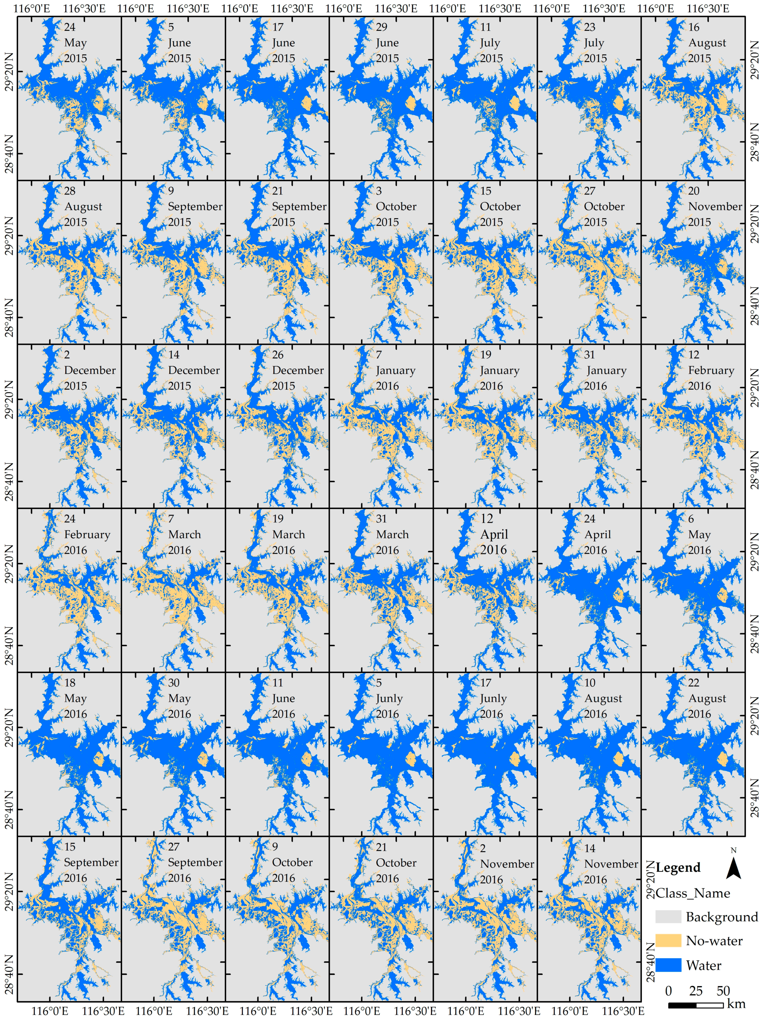
Figure 3.
Spatiotemporal distribution of surface water in Poyang Lake based on the SWI from 24 May 2015 to 14 November 2016. The interval of the time-series was 12 days and there were 38 periods in total; however, five periods (4 August 2015; 8 November 2015; 23 June 2016; 29 July 2016; and 3 September 2016) were missing due to a lack of Sentinel-1A data. The yellow color represents non-water and the blue color represents water.
Figure 4.
The area of Poyang Lake from 24 May 2015 to 14 November 2016, with intervals of 12 days.
Figure 4.
The area of Poyang Lake from 24 May 2015 to 14 November 2016, with intervals of 12 days.
Figure 5.
The examined SWI classification accuracy based on OLI: (a) OLI true color (R band 4, G band 3, B band 2) imagery acquired on 27 September 2016 located in Poyang Lake; (b) classification results based on Sentinel-1A imagery acquired on 27 September 2016; (c) SWI classification accuracy based on OLI on 27 September 2016; (d) OLI true color imagery acquired on 9 September 2015 located in Poyang Lake; (e) classification results based on Sentinel-1A imagery acquired on 9 September 2015; (f) SWI classification accuracy based on OLI on 9 September 2015; (g) OLI true color imagery acquired on 2 February 2016 located in Taihu Lake, China; (h) classification results based on Sentinel-1A imagery acquired on 2 February 2016; and (i) SWI classification accuracy based on OLI on 2 February 2016.
Figure 6.
Submergence ratios in Poyang Lake from 24 May 2015 to 14 November 2016. The red line shows the boundary of the sub-region. Poyang Lake was divided into Regions I–IV based on the submergence ratio to describe the changed characteristics in different regions.
Figure 6.
Submergence ratios in Poyang Lake from 24 May 2015 to 14 November 2016. The red line shows the boundary of the sub-region. Poyang Lake was divided into Regions I–IV based on the submergence ratio to describe the changed characteristics in different regions.
Figure 7.
The number of lakes with different areas that constitute the Poyang Lake. The black line represents the lakes with an area of 0.1–1 km2, the red line represents the lakes with an area of >1–10 km2, and the blue line represents the lake with area of >10–100 km2. The background color is used to distinguish the rainy season and dry season: the light green color represents the rainy season, and the light yellow color represents the dry season.
Figure 8.
Water surface area extracted from SWI and OLI from 24 May 2015 to 14 November 2016.
Figure 8.
Water surface area extracted from SWI and OLI from 24 May 2015 to 14 November 2016.
Figure 9.
MODIS classification accuracy based on OLI.
Figure 9.
MODIS classification accuracy based on OLI.
Figure 10.
The surface features in OLI of the commission and omission of water extracted from SWI images: (a) and (b) OLI true color (R band 4, G band 3, B band 2) imagery acquired on 9 September 2015.
Figure 10.
The surface features in OLI of the commission and omission of water extracted from SWI images: (a) and (b) OLI true color (R band 4, G band 3, B band 2) imagery acquired on 9 September 2015.
Figure 11.
The spectral characteristic of misclassified zones and normal vegetation and water regarded as references in OLI on 9 September 2015.
Figure 11.
The spectral characteristic of misclassified zones and normal vegetation and water regarded as references in OLI on 9 September 2015.
Table 1.
Examination of the Sentinel-1A water index equation using indexes.
Table 1.
Examination of the Sentinel-1A water index equation using indexes.
| Region | Date | Number of Pixels | RMSE | MAE | RMAPE (%) | R2 |
|---|
| Poyang Lake | 9 September 2015 | 225 | 0.21 | 0.17 | 3.99 | 0.92 |
| Taihu Lake | 2 February 2016 | 190 | 0.32 | 0.21 | 5.32 | 0.92 |
Table 2.
Confusion matrix for the SWI classification accuracy.
Table 2.
Confusion matrix for the SWI classification accuracy.
| Region and Date | Category | QA (%) | PA (%) | UA (%) | OA (%) | Kappa |
|---|
| Poyang Lake, 27 September 2016 | Water | 98.84 | 91.51 | 92.58 | 96.52 | 0.8981 |
| Non-water | 99.67 | 97.93 | 97.61 |
| Poyang Lake, 9 September 2015 | Water | 99.18 | 94.18 | 93.41 | 96.16 | 0.9102 |
| Non-water | 99.64 | 97.05 | 97.40 |
| Taihu Lake, 2 February 2016 | Water | 98.51 | 97.16 | 98.73 | 98.62 | 0.9690 |
| Non-water | 99.19 | 99.37 | 98.57 |
Table 3.
The accuracy of water extraction using different methods and datasets acquired on 27 September 2016.
Table 3.
The accuracy of water extraction using different methods and datasets acquired on 27 September 2016.
| Category Method | Data | Accuracy of Water (%) | Running Time (s) |
|---|
| QA | OA | UA | PA | Kappa |
|---|
| Threshold Classification Method (TCM) | SWI | 98.84 | 96.52 | 92.58 | 91.51 | 0.90 | 2 |
| VH | 93.02 | 94.50 | 85.07 | 91.01 | 0.84 | 2 |
| VV | 94.38 | 95.99 | 93.35 | 88.10 | 0.88 | 2 |
| VH and VV | 87.05 | 94.52 | 83.25 | 94.03 | 0.85 | 3 |
| IsoData Unsupervised Classification (IUC) | SWI | 98.01 | 96.55 | 93.03 | 91.18 | 0.90 | 4 |
| VH | 46.01 | 87.39 | 63.89 | 98.38 | 0.69 | 4 |
| VV | 79.37 | 92.57 | 77.48 | 93.46 | 0.80 | 4 |
| VH and VV | 72.27 | 92.27 | 75.40 | 96.31 | 0.80 | 5 |
| Minimum Distance Classification (MDC) | SWI | 96.38 | 96.59 | 93.85 | 90.45 | 0.90 | 3 |
| VH | 82.07 | 93.58 | 80.04 | 94.40 | 0.82 | 3 |
| VV | 94.78 | 95.15 | 87.06 | 91.61 | 0.86 | 3 |
| VH and VV | 96.66 | 96.06 | 89.74 | 92.73 | 0.89 | 3 |
| Support Vector Machine (SVM) | SWI | 99.57 | 96.42 | 91.69 | 92.08 | 0.90 | 13 |
| VH | 97.11 | 94.58 | 86.65 | 89.16 | 0.84 | 193 |
| VV | 94.63 | 95.13 | 86.96 | 91.63 | 0.86 | 52 |
| VH and VV | 97.84 | 96.19 | 90.49 | 92.44 | 0.89 | 18 |
© 2017 by the authors. Licensee MDPI, Basel, Switzerland. This article is an open access article distributed under the terms and conditions of the Creative Commons Attribution (CC BY) license (http://creativecommons.org/licenses/by/4.0/).


 ,
, 


