Identifying Irrigated Areas in the Snake River Plain, Idaho: Evaluating Performance across Composting Algorithms, Spectral Indices, and Sensors

Abstract

There are pressing concerns about the interplay between agricultural productivity, water demand, and water availability in semi-arid to arid regions of the world. Currently, irrigated agriculture is the dominant water user in these regions and is estimated to consume approximately 80% of the world’s diverted freshwater resources. We develop an improved irrigated land-use mapping algorithm that uses the seasonal maximum value of a spectral index to distinguish between irrigated and non-irrigated parcels in Idaho’s Snake River Plain. We compare this approach to two alternative algorithms that differentiate between irrigated and non-irrigated parcels using spectral index values at a single date or the area beneath spectral index trajectories for the duration of the agricultural growing season. Using six different pixel and county-scale error metrics, we evaluate the performance of these three algorithms across all possible combinations of two growing seasons (2002 and 2007), two datasets (MODIS and Landsat 5), and three spectral indices, the Normalized Difference Vegetation Index, Enhanced Vegetation Index and Normalized Difference Moisture Index (NDVI, EVI, and NDMI). We demonstrate that, on average, the seasonal-maximum algorithm yields an improvement in classification accuracy over the accepted single-date approach, and that the average improvement under this approach is a 60% reduction in county scale root mean square error (RMSE), and modest improvements of overall accuracy in the pixel scale validation. The greater accuracy of the seasonal-maximum algorithm is primarily due to its ability to correctly classify non-irrigated lands in riparian and developed areas of the study region.

1. Introduction

Semi-arid and arid regions cover nearly 41% of the Earth’s surface and are home to more than 38% of the population [1]. These regions typically receive limited precipitation during the agricultural growing season of April to October, averaging 0.1–0.8 m annually, and experience hotter, drier summers than other regions of the world [2]. Most vegetation is likely to be dead or in a stage of senescence during the hot summer months unless supplemental water is available for plant consumption. As a result, semi-arid and arid regions rely heavily on irrigation to support agriculture. For example, in the western United States, agriculture accounts for over 90% of consumptive groundwater and surface water use [3]. The 17 conterminous western states alone account for 85% of water withdrawals in the United States and 74% of irrigated acres, with the states of California, Texas, and Idaho consistently leading the nation in total water withdrawals [3]. Given the reliance of these regions on irrigation, it is essential to develop an understanding of spatial and temporal patterns of water use and food production. In addition to the food security implications, use of irrigation in the agricultural landscape is of particular interest because it affects groundwater quality and quantity, ecological processes, climate, and biogeochemical and hydrologic cycles [4].

Accurate mapping of the distribution of irrigated land at a regional scale can facilitate an improved understanding of patterns of water use and food production on an annual to decadal basis. As the frequency of precipitation events declines during the summer months, anomalies in plant greenness or water content can be attributed to irrigation practices. Specifically, the presence of green, healthy vegetation during the summer growing season can most likely be attributed to irrigation water applications [5]. Remote sensing yields a source of readily available data that can be used to identify and quantify irrigated area on an annual timescale based on within-season trends in greenness. In particular, the Normalized Difference Vegetation Index (NDVI), derived using near infrared and red reflectance, has been used for mapping irrigated areas on the local scale and is effective because of differential spectral responses between irrigated and non-irrigated croplands [6].

Using NDVI as an indicator of vegetation phenology reduces the amount of computational storage needed, improves processing time, and provides a simple means for classifying complex landscapes [7]. There is overwhelming agreement that NDVI can be a vegetation monitoring tool [8,9,10,11]. NDVI and plant moisture availability are closely related [12], which makes NDVI a sufficiently good indicator of irrigation presence [13,14,15,16]. Studies using NDVI have been used to distinguish irrigated from non-irrigated land use in semi-arid and arid regions in India and Turkey [5,7,17]. NDVI has also been used to classify land use and land cover in which irrigated area is one of multiple classification categories [4,18,19].

Moderate Resolution Imaging Spectroradiometer (MODIS) and Landsat have been found to be the most effective imagery for observing differences in NDVI in semi-arid and arid regions [6]. The MODIS instrument, aboard NASA’s Aqua and Terra satellites, has been applied to map land use using multiple reflectance spectra and vegetation indices [17,20]. Likewise, the Landsat remote sensing system has proven a useful tool for producing land-use maps [21,22]. Each of these remote sensing products has its spatial and temporal advantages and disadvantages: MODIS gathers higher-frequency, daily data, but at a relatively coarse, 250-m or 500-m spatial resolution, whereas Landsat has a lower-frequency return interval of approximately 16 days, but a relatively fine, 30-m spatial resolution. A shorter return interval is advantageous when cloud cover renders some images during the agricultural growing season unusable; a finer spatial resolution is advantageous because it captures water use patterns at the scale of the individual field.

Ozdogan et al. [5,6] demonstrate that using a single observation date for NDVI, preferably during the peak of the growing season, is sufficient for distinguishing irrigated from non-irrigated land use using Landsat data in southeastern Turkey. When applying this method to other regions, however, classification errors may arise if farmers use inconsistent harvesting and irrigation practices. For example, alfalfa may be harvested multiple times throughout the growing season, potentially lowering its NDVI (and other index) values just after harvest. Likewise, irrigated water may have been cut off before the selected single image date, again potentially lowering NDVI values. Moreover, the optimal choice of observation date may differ across space and across years due to differences in summer precipitation events, for example.

To address these challenges, we test methods that have the potential to identify areas that are irrigated at any point throughout the entire growing season. We thus introduce methods that extend the window of observation from a single date to a time interval that captures within-season differences in greenness trajectories between irrigated and non-irrigated sites. We evaluate two new algorithms and the existing, single-date algorithm from Ozdogan et al. [5,6] for classifying irrigated lands in semi-arid and arid regions using multispectral data from both MODIS and Landsat. The two new algorithms classify land use based on summary statistics that describe the trajectory of greenness over the duration of the growing season (April to October). The first, which we call the greenness-duration approach, develops a threshold based on the difference in area below the spectral index curve for irrigated and non-irrigated sites. The second, which we call the seasonal maximum approach, develops a threshold based on the difference in the maximum of each spectral index between irrigated and non-irrigated sites (where the maximum for each index may fall on a different date). These new algorithms and the single-date algorithm are implemented using three vegetation indices—The Normalized Difference Vegetation Index (NDVI), Enhanced Vegetation Index (EVI), and the Normalized Difference Moisture Index (NDMI)—derived from both MODIS and Landsat imagery. Our objective is to contrast the performance of each algorithm-spectral index-dataset combination in terms of classification accuracy and to quantify the spatiotemporal patterns of irrigated land in our study region.

2. Study Region

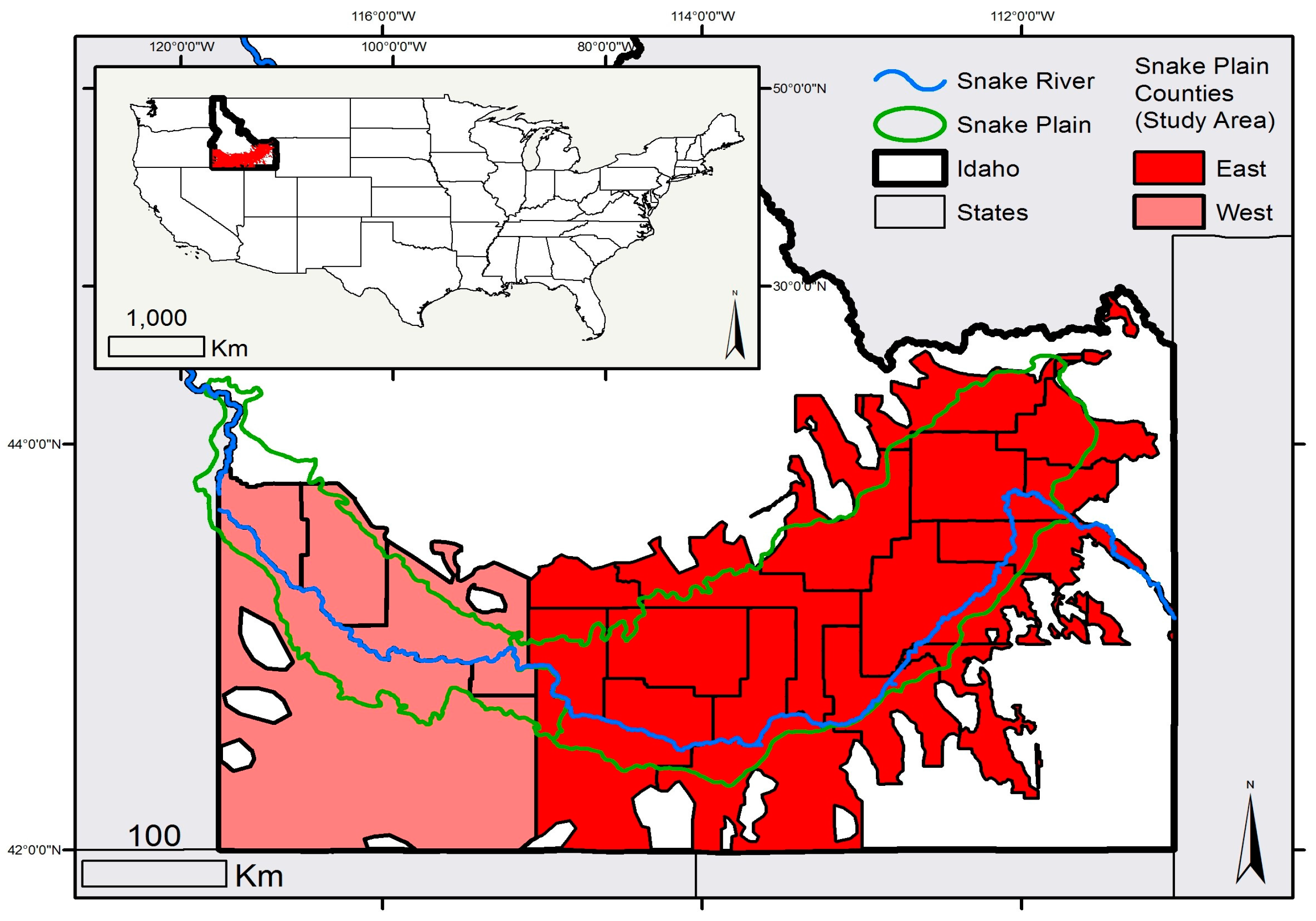
Our study region is the counties containing the Snake River Plain (SRP) of Idaho, United States (Figure 1). The region is approximately 500 km east to west, and spans the majority of southern Idaho. The SRP has a Mediterranean-style semi-arid to arid climate in which the summer months have lower precipitation compared to other months of the year. The entire study area exhibits a “summer dry” climate, which allows us to explore methods to map irrigated land use via changes to the Earth’s surface reflectance spectra caused by irrigation. However, there are significant differences in elevation, temperatures, and precipitation between the western and eastern SRP (distinguished by a black line in Figure 1). Relative to the eastern portion of the SRP, the western portion is at a higher elevation, with generally higher temperatures and more precipitation. Mean annual temperature is at its maximum in the western portion of the Snake Plain at 13 °C, and precipitation generally increases west to east from approximately 25 cm annually to 35 cm annually, the majority of this comes during winter months. Much lower temperatures and higher precipitations occur on the surrounding mountains. Elevations of the plain vary from approximately 680 m above sea level in the west to 1680 m in the east (higher elevations can be found in adjacent mountain peaks, several of which are in excess of 2800 m). Differences in climate between the eastern and western portions of the SRP are primarily controlled by Pacific Ocean-derived moisture and topography [23].

In the SRP, agricultural productivity, the value of agricultural land, and farmers’ land-use decisions are driven by the availability of water for irrigation. Idaho alone ranks third in the United States in terms of the volume of water withdrawn, and first in terms of water withdrawals per capita [24]. Over 98% of all water withdrawn in Idaho goes to counties that lie completely or partially within the SRP, with the majority of that water, 85.6%, used for irrigation [25]. Based on the 2011 USDA Cropland Data Layer, within the SRP’s cultivated lands 28% was growing spring and winter wheat, 26% was alfalfa, 12% was barley, 10% was corn, 10% was potato, 6% was sugar beet, 2% was dry beans and 4% was growing other crops. Approximately 20% of the study region is in agriculture. Water for irrigation is supplied predominantly by winter snowpack, rendering this region particularly vulnerable to the effects of climate change [26]. Recent research shows that climate has already begun to impact the timing of snowmelt runoff and suggests increased variability in the timing and magnitude of available water derived from winter snowmelt in the future [27]. Increased variability in water resources during the late summer months, at a time when water is critical for crop growth, will introduce uncertainty into agricultural production. This uncertainty is likely to influence land-use patterns, and thus the economy, hydrology, and ecology of the region.

3. Materials and Methods

As is evident in Figure 1, our study area is relatively large and encompasses multiple Landsat scenes (i.e., Landsat paths 38–42 and rows 29–31). For the multitemporal Landsat analysis, this introduces “big data” computational challenges, with large data volumes (terabytes) and high performance computing requirements for image processing. Therefore, we utilize the Google Earth Engine API platform for our multitemporal algorithms. As part of the platform, Google maintains the Landsat and MODIS satellite archives, with Landsat data pre-processed to reflectance. Using this interface, we use the Landsat reflectance products with masked clouds identified by the Fmask algorithm [28]. Our index calculations and algorithm computations are also performed in this environment.

3.1. Vegetation and Plant-Water Indices at High and Moderate Spatial Resolutions

This study classifies irrigated land using two common vegetation mapping indices (i.e., NDVI and EVI) and a plant–water index, NDMI, which is designed to be more sensitive to changes in canopy water content.

NDVI is defined as:

$$\mathrm{NDVI}=\frac{{\mathsf{\rho }}_{\mathrm{nir}}-{\mathsf{\rho }}_{\mathrm{red}}}{{\mathsf{\rho }}_{\mathrm{nir}}+{\mathsf{\rho }}_{\mathrm{red}}}$$

(1)

where ρ_nir and ρ_red represent near infrared and red reflectances, respectively [29]. EVI is a refined version of NDVI that corrects for additional atmospheric influences, reduces saturation, and accounts for canopy effects [20,30,31]. EVI is defined as:

$$\mathrm{EVI}=\mathrm{G}\times \frac{\left({\mathsf{\rho }}_{\mathrm{nir}}-{\mathsf{\rho }}_{\mathrm{red}}\right)}{\left({\mathsf{\rho }}_{\mathrm{nir}}+\mathrm{C}1\times {\mathsf{\rho }}_{\mathrm{red}}-\mathrm{C}2\times {\mathsf{\rho }}_{\mathrm{blue}}+\mathrm{L}\right)}$$

(2)

where G, C1, C2 and L are sensor-specific constants for gain (G), aerosol resistance (C1 and C2), and a canopy adjustment term (L).

NDMI, also referred to as the Normalized Difference Water Index (NDWI), is defined as:

$$\mathrm{NDMI}=\frac{{\mathsf{\rho }}_{\mathrm{nir}}-{\mathsf{\rho }}_{\mathrm{swir}1}}{{\mathsf{\rho }}_{\mathrm{nir}}+{\mathsf{\rho }}_{\mathrm{swir}1}}$$

(3)

where ρ_swir1 represents short wave infrared (1.55–1.75 μm) reflectance [32].

We calculate each index at high (Landsat, 30-m) and moderate (MODIS, 250-m and 500-m) spatial resolution.

Table 1. Summary of remote sensing products tested including data provider, dataset name, compositing description, and spatial resolution.

		Single Date	Greenness-Duration	Seasonal Maximum
MODIS	NDVI	NASA/USGS, MOD13Q1, 16-Day SR mosaic, 250-m
	EVI
	NDMI	Google, MCD43A4, 16 day SR mosaic, 500-m
Landsat 5	NDVI	Google, 32 day TOA mosaic, 30-m
	EVI
	NDMI	-	USGS, non-composited SR, 30-m

provides a summary of the data products used in this study. The MODIS global data product (MOD13Q1) includes cloud-free 16-day mosaics of NDVI and EVI. Landsat 5 surface reflectance (SR) data were used to provide high resolution versions of NDVI, EVI, and NDMI. Existing NDVI, EVI, and NDMI cloud-free 32-day top of atmosphere (TOA) composites were used (LT5_L1T_32DAY, provided by Google Earth Engine). It should be noted that the size of the study area necessitated using images composited over several days for the single date approach in order to get a single image that covers the study area. In addition, the Google composites generally use the most recent image in the given time period unless it is cloud impacted.

Table A1. Threshold values for each year and algorithm. Producer’s and user’s accuracies are for the irrigated class.

Dataset	Index	Aggregation Algorithm	Threshold		Single Date Composite Start
			2002	2007	2002	2007
MODIS	NDVI	Single Date	5000	4026	8/13	7/28
		Greenness-Duration	4307	4276
		Maximum	7849	7479
	EVI	Single Date	3458	2802	7/28	6/10
		Greenness-Duration	3125	3021
		Maximum	6672	5740
	NDMI	Single Date	−0.0302	−0.0313	7/12	7/4
		Greenness-Duration	−0.0422	−0.0495
		Maximum	0.0979	0.0432
Landsat 5	NDVI	Single Date	0.3953	0.3286	6/10	6/10
		Greenness-Duration	0.2521	0.3099
		Maximum	0.5745	0.6036
	EVI	Single Date	0.3286	0.2656	6/10	6/10
		Greenness-Duration	0.2313	0.2745
		Maximum	0.5411	0.5552
	NDMI	Single Date	0.0771	0.0260	6/10	6/10
		Greenness-Duration	0.0516	0.0297
		Maximum	0.3922	0.3318
		Maximum3×3	0.3375	0.3385

Notes: Some of the data products used have values scaled by 10,000 so the resulting thresholds are also scaled. Single date methods used 16 and 32 day composites, dates listed are the starting date of each composite (month/day).

lists the start date of each composite used.

3.2. Development of a Training Dataset

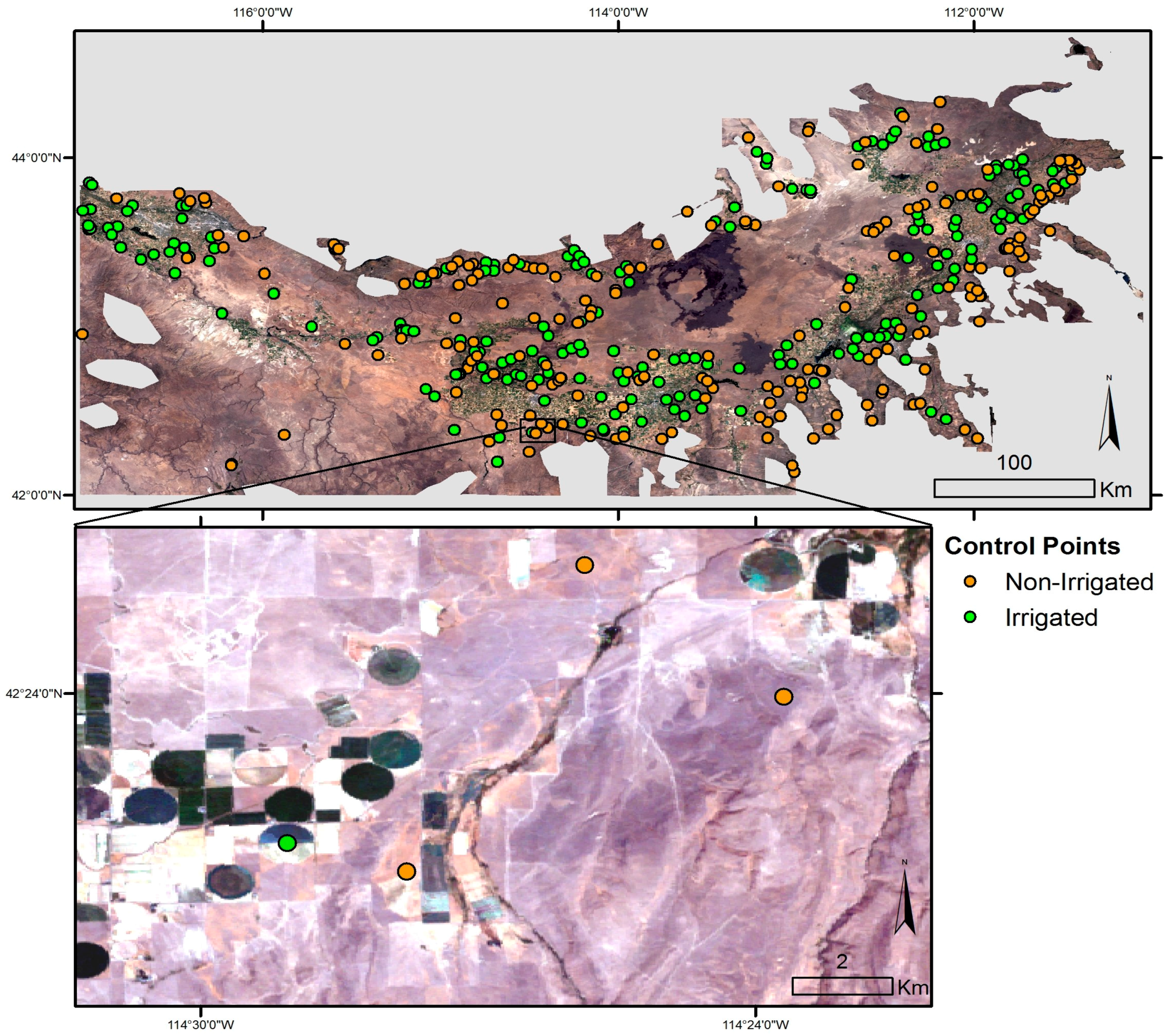
A training dataset of known land-use points was developed using manual interpretation of the National Agriculture Imagery Product (NAIP), which consists of high resolution aerial photographs. In our study region, NAIP images are available for the 2003, 2004, 2006, and 2009 growing seasons. Approximately 10 irrigated and 10 non-irrigated points were identified within each of 21 counties. The final training dataset contains a total of 404 control points. Points were generally located near the center of fields or away from edge areas to avoid mixed pixels, however for the at the 500 m resolution of some of the MODIS data some mixing is likely inevitable. Figure 2 illustrates these control points as well as several example points for Twin Falls County in 2007.

3.3. Three Pixel-Scale Thresholding Approaches for Classification

We investigate three classification algorithms using each of the spectral indices (NDVI, EVI and NDMI) developed using data from MODIS and Landsat 5. Each algorithm is implemented for two years—the 2002 and 2007 growing seasons. The classification itself is performed at the scale of the individual pixel. We report classification accuracy metrics at this spatial scale for each algorithm-index-dataset combination. In addition, the years 2002 and 2007 correspond to the years of the USDA Agricultural Census, which allows us to use aggregate, county level statistics as a second benchmark against which we test the classification accuracy of each algorithm-spectral index-dataset combination.

3.3.1. Single-Date Algorithm

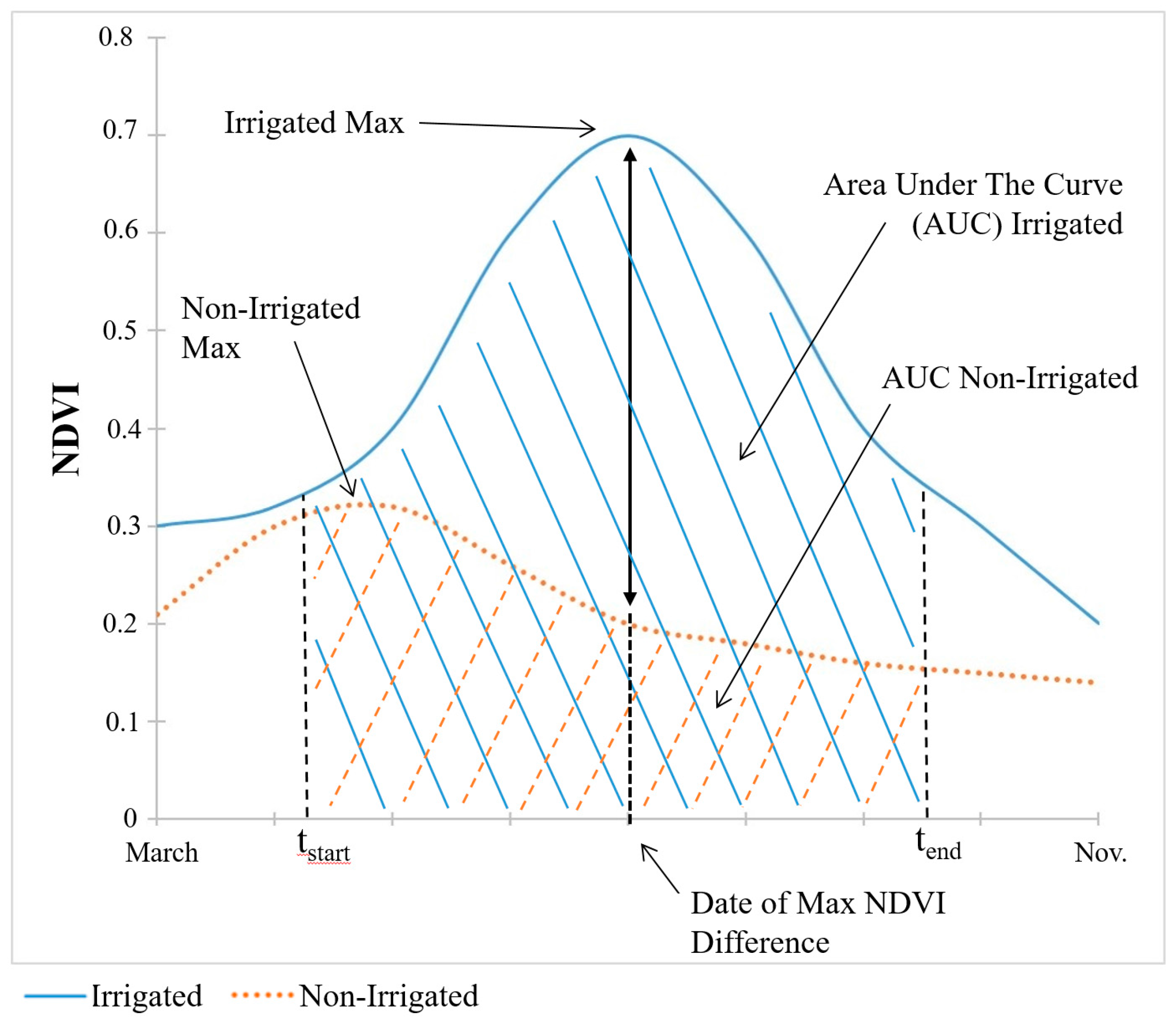
The first algorithm uses single-date imagery, as in Ozdogan et al. [5,6]. This method requires that we first determine the observation date at which the difference in the spectral index value between irrigated and non-irrigated land is at its maximum. The date at which the maximum difference in the spectral index between irrigated and non-irrigated pixels is observed is illustrated conceptually for NDVI by the vertical black arrow in Figure 3 (the conceptual diagram is the same for EVI and NDMI). For each year we select the composite image for which the irrigated and non-irrigated index values are at their greatest separation by calculating the difference between the sum of all spectral index values for the training dataset of known irrigated points and the sum for non-irrigated points for each available image date within the growing season. As discussed by Ozdogan et al. [5], the best window to apply this classification scheme is near the timing of peak green-up.

We then derive a threshold value that maximizes classification accuracy for both land-use categories. To do so, we fit a separate nonparametric kernel density function to the observed spectral index values for irrigated and non-irrigated control points in the training dataset. This is done using the kdensity function in Matlab, which uses a frequency of 1/100th the range of the data. Using those fitted distributions, we calculate the probability that a pixel is irrigated or non-irrigated at a range of potential threshold values based on both kernel density functions. We select the threshold value at which the probability of classifying the pixel as irrigated or non-irrigated is equal, which represents the point at which the fitted normal kernel density functions intersect (which simultaneously minimizes type II error for both distributions). Observations above the threshold are classified as irrigated; those below the threshold are classified as non-irrigated. Threshold values used for each year and classification method are listed in Appendix A (Table A1).

3.3.2. Greenness-Duration Algorithm

The second thresholding method distinguishes irrigated from non-irrigated land using the area under a spectral index curve over the duration of the growing season, rather than at a single date. The differences in the areas under the spectral index curve for irrigated and non-irrigated points are illustrated for NDVI with cross-hatching in Figure 3. The area under each spectral index curve is computed by calculating the integral of the time series from 1 April to 31 October and deriving the threshold value that most accurately classifies both land-use categories using the same probability based approach used for the single-date algorithm.

Peak green-up, the time at which crops are at or nearly at their maximum index values, typically occurs in mid-summer. However, using the greenness-duration approach, we find that the greatest difference in the areas under the spectral index curves tends to fall later in the growing season. This occurs because following peak green-up, non-irrigated crops typically begin to show a reduction in vegetation index values while irrigated control point values maintain elevated levels for multiple images.

This approach also mitigates some classification error that arises when crops are harvested multiple times during the growing season, such as alfalfa, which is one of the top crops grown in the SRP. Irrigated alfalfa may be harvested 4–5 times during a growing season, while dryland alfalfa yields fewer cuttings. Multiple cuttings result in multiple peaks in spectral indices during the growing season, muddying the signal in peak green-up for the single-date approach. By accounting for the area under the curves, the greenness-duration approach better captures the difference in spectral index for irrigated and non-irrigated crops across multiple cuttings.

3.3.3. Seasonal-Maximum Algorithm

In our third approach, we use a single threshold value for the region based on the seasonal maximum for each spectral index, where both the date and the level of the seasonal maximum of irrigated crops may differ from that of non-irrigated crops, as illustrated in Figure 3. We compute the seasonal maximum for each growing season (again defined as 1 April to 31 October) in Google Earth Engine. Here we use the same probability based approach to select the optimal threshold as described for the single-date and greenness-duration algorithms.

When using the Landsat NDMI data for this algorithm, error may be introduced into the classification due to variability in NDMI from climate, farm equipment, or other anomalies. To address this challenge and increase the reliability of the training dataset for this particular algorithm-index-dataset combination, we extract a nine-pixel square around each control point. We remove from the dataset any pixel values outside two standard deviations of the mean NDMI within the nine-pixel square. We also control for differences in climate across the study region through the inclusion of average annual precipitation data for each control point or nine-pixel square [33]. We use average precipitation data because spatially explicit annual precipitation data are not available for the entire study period. Using discriminant analysis for the 2003 growing season, we test the effect of controlling for precipitation.

3.4. Validation and Accuracy Assessment

We validate the classification from each algorithm-index-dataset combination at the individual pixel level using two different validation datasets. The first (which we refer to as the symmetrical validation dataset) uses 75 known irrigated and 75 known non-irrigated points. The second validation dataset (which we refer to as the supplemental land-use validation dataset) uses NAIP imagery to differentiate between irrigated land and multiple non-irrigated land uses, including dryland agriculture and development. In addition to these pixel-scale validation approaches, we compare the classified area in irrigated and dryland agriculture to county level statistics from the USDA Census of Agriculture.

For the pixel-scale symmetrical validation dataset, we create a sample dataset of randomly selected points in the region and determine whether they are irrigated or non-irrigated agriculture in 2002 and 2007 using NAIP and Google Earth imagery. We supplement this dataset with randomly generated points that lie within the geospatial boundaries of the place of use for prior appropriation water rights [34]. Farmers are restricted to applying water for irrigation within the place of use specified as part of a water right [35,36]. Using these supplementary data facilitate the process of identifying control points that are irrigated. Large forested areas, which mainly occur along the outer edge of the study region, are hand-delineated and removed from the analysis to attain an appropriate measure of accuracy in classifying irrigated area. In comparison to irrigated NDVI trends, the NDVI values of forested locations show far less variability than irrigated land use over the same time period.

From a randomly selected sample of potential validation points, we exclude points that were primarily in agricultural areas that appeared, based on NAIP imagery, to have been non-irrigated at some point between 2002 and 2007. In addition, we exclude points for which it is unclear whether they are irrigated or non-irrigated. Examples include areas with visible irrigation infrastructure where the crops appeared non-irrigated or areas where no visible irrigation infrastructure was present but the crops were greener than nearby nonagricultural areas. We also exclude points that are close to the edge of a field or points that contain multiple land-use types. The final pixel-level symmetrical validation dataset contains 150 points (75 irrigated and 75 non-irrigated) that can be definitively identified as irrigated or non-irrigated for our entire study period. We use these selected points to generate a confusion matrix with commonly used classification accuracy metrics, including overall accuracy, user’s accuracy, producer’s accuracy, and the kappa coefficient, as a comparison of the observed accuracy to random chance.

For the pixel-scale supplementary land use validation dataset, we randomly select 320 points in the study region, 20% of which are irrigated or dryland agriculture, and 3% of which are suburban or urban development. This land-use composition is representative of the region based on the 2006 National Land Cover Dataset [37]. We use NAIP imagery to determine land cover for 2007, but areas that are not irrigated are broken down into four classes: desert (sparsely vegetated), non-agricultural but vegetated (green areas, usually riparian or covered with woody vegetation), dryland (non-irrigated) agriculture, and developed (urban and suburban areas). Points are only adjusted if they were too close to the edge of a field, or to ensure that there were representative proportions of agriculture, non-agriculture, and developed lands (20% agriculture, 3% developed and 77% other). The percentage of points correctly classified in each of these categories is calculated, as well as the overall percent correctly classified.

As an additional assessment of our results, we compare our findings to data from the USDA Census of Agriculture. Here, we calculate irrigated and non-irrigated areas by county for each year and compare our area total to that from the USDA Census of Agriculture for the years 2002 and 2007. The Census data are based on surveys of individual farmers, but is reported at the county scale. This provides an independent third-party assessment of our algorithm-index-dataset combinations. We compute the coefficient of determination (R²) as an indication of the variance of the area reported in the Census that is explained by our model outputs. We also report the root mean squared error (RMSE) as a measure of the difference in predicted irrigated area relative to USDA Census statistics.

4. Results

With a combination of three algorithms (single date, greenness duration, and seasonal maximum), three spectral indices (NDVI, EVI, and NDMI), two remote sensing datasets (Landsat 5 and MODIS), and two years (2002 and 2007), the results from this analysis (36 products) are too numerous to fully display here. Instead, we present summary statistics describing classification accuracy for all cases using the pixel-scale symmetrical validation dataset and county scale Census data in

Table 2. Single-date algorithm accuracy statistics. Producer’s and user’s accuracies are for the irrigated class. Coefficient of determination (R²) and root mean square error (RMSE) are calculated at the county scale.

Year	Dataset	Index	Pixel Scale				County Scale
			Overall Accuracy (%)	Producer’s Accuracy (%)	User’s Accuracy (%)	Kappa	R2	RMSE (km2)
2002	Landsat	NDVI	90.0	81.3	98.4	0.800	0.676	281
		EVI	92.0	84.0	100.0	0.840	0.771	237
		NDMI	97.3	97.3	97.3	0.947	0.839	350
	MODIS	NDVI	86.0	72.0	100.0	0.720	0.893	118
		EVI	87.3	74.7	100.0	0.747	0.910	160
		NDMI	96.0	94.7	97.3	0.920	0.920	298
2007	Landsat	NDVI	99.3	98.7	100.0	0.987	0.733	309
		EVI	99.3	98.7	100.0	0.987	0.838	268
		NDMI	91.3	84.0	98.4	0.827	0.777	290
	MODIS	NDVI	89.3	80.0	98.4	0.787	0.873	300
		EVI	98.7	98.7	98.7	0.973	0.757	490
		NDMI	96.0	94.7	97.3	0.920	0.948	255

,

Table 3. Percent change in accuracy for greenness-duration algorithm relative to single-date algorithm. Producer’s and user’s accuracies are for the irrigated class.

Year	Dataset	Index	Pixel Scale				County Scale
			Overall Accuracy (%)	Producer’s Accuracy (%)	User’s Accuracy (%)	Kappa	R2	RMSE (km2)
2002	Landsat	NDVI	3.7	8.2	0.1	8.3	18.6	4.9
		EVI	3.6	7.9	0.0	7.9	17.1	−7.1
		NDMI	0.7	0.0	1.4	1.4	12.3	−42.0
	MODIS	NDVI	10.1	24.1	0.0	24.1	−3.1	171.4
		EVI	9.9	23.2	0.0	23.2	6.6	15.1
		NDMI	0.0	−2.8	2.8	0.0	2.6	−19.7
2007	Landsat	NDVI	−0.7	−1.4	0.0	−1.4	22.8	−35.5
		EVI	−0.7	−1.4	0.0	−1.4	13.8	−44.8
		NDMI	8.8	19.0	0.3	19.4	19.9	−26.6
	MODIS	NDVI	9.7	20.0	1.7	22.0	1.1	5.0
		EVI	0.0	−1.4	1.4	0.0	26.3	−58.1
		NDMI	1.4	0.0	2.8	2.9	−2.1	−4.9
Average			3.9	8.0	0.9	8.9	11.3	−3.5
Standard Deviation			4.3	10.3	1.1	9.9	9.6	57.1

Notes: Percent changes are calculated relative to the accuracy statistic presented in the corresponding cell of Table 2. Accuracy statistic levels for the greenness-duration algorithm are reported in the Appendix in Table A2. Pixel scale significance levels are reported in the Appendix in Table A4 and Table A5 for comparisons across compositing algorithms and spectral indices. All differences in county scale performance are significant based on a z score test and a critical level of 0.05.

and

Table 4. Percent change in accuracy for seasonal-maximum algorithm relative to single-date algorithm. Producer’s and user’s accuracies are for the irrigated class.

Year	Dataset	Index	Pixel Scale				County Scale
			Overall Accuracy (%)	Producer’s Accuracy (%)	User’s Accuracy (%)	Kappa	R2	RMSE (km2)
2002	Landsat	NDVI	7.4	14.8	1.6	16.7	37.5	−62.1
		EVI	6.5	14.3	0.0	14.3	23.5	−65.2
		NDMI	−1.4	−5.5	2.7	−2.8	16.3	−82.7
		NDMI3×3	0.7	−1.4	2.7	1.4	15.7	−81.0
	MODIS	NDVI	7.8	20.4	−1.5	18.5	−9.1	22.8
		EVI	6.9	17.9	−1.5	16.1	2.0	−40.7
		NDMI *	−6.9	−15.5	1.1	−14.5	−53.5	−3.9
2007	Landsat	NDVI	−1.3	−2.7	0.0	−2.7	30.9	−78.3
		EVI	−1.3	−2.7	0.0	−2.7	16.5	−81.1
		NDMI	8.0	15.9	1.6	17.7	26.2	−83.7
		NDMI3×3	8.0	15.9	1.6	17.7	26.2	−84.4
	MODIS	NDVI	9.7	20.0	1.7	22.0	6.7	−70.2
		EVI	0.0	−1.4	1.4	0.0	29.1	−80.5
		NDMI	0.7	−1.4	2.8	1.4	3.1	−49.2
Average			3.2	6.3	1.0	7.4	12.2	−60.0
Standard Deviation			4.9	11.3	1.4	10.9	22.1	31.6

Notes: Percent changes are calculated relative to the accuracy statistic presented in the corresponding cell of Table 2. Accuracy statistic levels for the seasonal-maximum algorithm are reported in the Appendix in Table A3. Pixel scale significance levels are reported in the Appendix in Table A4 and Table A5 for comparisons across compositing algorithms and spectral indices. All differences in county scale performance are significant based on a z score test and a critical level of 0.05. * The 2002 MODIS NDMI Google composite images contain several large sections of unmasked clouds, lowering the accuracy of the calculated threshold in this instance.

and the supplementary pixel-scale land use validation dataset in

Table 5. Percent change in pixel scale overall accuracy for greenness-duration (GD) and seasonal-maximum (Max) algorithms relative to the single-date algorithm using supplementary land-use validation points for 2007.

Dataset	Index	Algorithm	% Correctly Classified
			Non-Irrigated				Irrigated Ag.	Total
			Desert	Non-Ag. Green Vegetation	Dry Ag.	Developed
MODIS	NDVI	GD	−0.5	−23.5	12.5	0.0	8.3	0.0
		Max	1.9	35.3	12.5	233.3	−6.3	5.2
	EVI	GD	−6.0	−27.3	−55.6	−50.0	−5.9	−10.1
		Max	0.9	9.1	11.1	25.0	−11.8	0.3
	NDMI	GD	0.0	0.0	0.0	−25.0	2.0	0.0
		Max	0.9	9.5	0.0	100.0	−8.0	1.3
Landsat	NDVI	GD	2.4	13.3	50.0	−28.6	0.0	2.8
		Max	4.3	53.3	83.3	42.9	−2.0	8.4
	EVI	GD	2.8	18.8	50.0	0.0	0.0	4.2
		Max	3.3	50.0	83.3	150.0	−4.0	8.3
	NDMI	GD	3.8	28.6	25.0	50.0	1.9	5.6
		Max	4.3	64.3	37.5	400.0	−1.9	9.8
		Max3×3	4.3	64.3	37.5	400.0	−1.9	9.8
Total Samples			220	24	12	10	54	320
Average, GD			0.4	1.6	13.7	−8.9	1.1	0.4
Standard Deviation, GD			3.2	20.9	35.9	31.5	4.2	5.1
Average, Max			2.8	40.8	37.9	193.0	−5.1	6.1
Standard Deviation, Max			1.5	21.9	31.5	145.7	3.5	3.7

Notes: Percent changes are calculated relative to the accuracy statistic for the single-date algorithm. Accuracy statistic levels for all algorithms are reported in the Appendix in Table A4.

. In addition, we present Landsat-derived NDMI maps of irrigated lands in 2007 for each of the three algorithms (Figure 4 and Figure 5). An equivalent to Figure 4 showing MODIS NDMI maps for 2007 is presented in Figure A1 in the Appendix. We choose this particular combination to map as a representative example of classification patterns produced by each classification algorithm.

4.1. Single-Date Algorithm

Figure 4A illustrates the 2007 Landsat-derived NDMI map using the single-date approach. The spatial pattern of irrigated lands produced by the algorithm corresponds to general spatial patterns in irrigated production throughout the study region. The majority of irrigated agricultural production follows the arc of the Snake River across the Plain. There are three predominant sub-regions in which irrigated production occurs: the northeastern portion of the Plain, fed by surface water flowing from the headwaters in Yellowstone National Park to the American Falls Reservoir; the south-central portion of the Plain (also called the Magic Valley), which is fed by springs from the Eastern Snake Plain Aquifer and extends to the western edge of the Eastern Snake Plain; and the Ada/Canyon County area in the northwestern corner of the Plain, which is home to much of the region’s specialized crop production, including viticulture and orchard crops. There are several linear artifacts in the northeast portion of Figure 4A that are a result of poor cloud removal in the 32 day composite created Google.

Table 2 presents pixel-level and county-level accuracy assessment statistics for the single-date algorithm by growing season, dataset, and spectral index. The pixel-level accuracy statistics are calculated using the symmetrical validation dataset. At the pixel scale, classifications based on Landsat data slightly outperform those produced with MODIS data across years and spectral indices. For example, using NDMI as the spectral index in 2002, the overall accuracy using Landsat is 97.3% with a kappa of 0.947; for MODIS, the corresponding statistics are 96% and 0.920. At the county scale, the opposite holds: the results favor a classification approach using MODIS data. For example, MODIS produces an R² of 0.920 and 0.948 for NDMI in 2002 and 2007, respectively, while Landsat produces an R² of 0.839 and 0.777 for the same index and years. The results using RMSE as a measure of county scale accuracy similarly favor MODIS, potentially because of MODIS’s higher temporal resolution, it may be more likely to capture an image closer to the date of peak greenness.

Across spectral indices, there are significant differences in classification accuracy (see Appendix

Table A4. p values for McNemar test of significance in difference between image compositing algorithms for the pixel scale classification accuracy. Values less than 0.05 are highlighted in light grey and those less than 0.01 are highlighted in dark grey.

Year	Dataset	Index	Single Date V. G.D.	Max. V. G.D.	Max. V. Single Date
2002	Landsat	NDVI	0.267	0.546	0.043
		EVI	0.228	0.221	0.016
		NDMI	1.000	0.131	0.077
		NDMI3×3		0.480	0.450
	MODIS	NDVI	0.004	1.000	0.031
		EVI	0.009	0.752	0.029
		NDMI *	0.221	0.043	0.001
2007	Landsat	NDVI	1.000	1.000	0.617
		EVI	1.000	1.000	0.617
		NDMI	0.001	0.248	0.027
		NDMI3×3		0.248	0.027
	MODIS	NDVI	0.006	0.480	0.016
		EVI	0.617	0.480	0.617
		NDMI	0.683	1.000	0.371

* The 2002 MODIS NDMI Google composite images contain several large sections of unmasked clouds, lowering the accuracy of the calculated threshold in this instance.

and

Table A5. p values for McNemar test of significance in difference between spectral indices for the pixel scale classification accuracy. Values less than 0.05 are highlighted in light grey and those less than 0.01 are highlighted in dark grey.

Year	Dataset	Index	NDVI V. EVI	NDMI V. EVI	NDMI V. NDVI
2002	Landsat	S.D.	1.000	0.003	0.004
		G.D.	1.000	0.041	0.046
		Max.	0.480	0.450	1.000
	MODIS	S.D.	0.752	0.001	0.000
		G.D.	0.752	0.752	0.752
		Max.	1.000	0.211	0.359
2007	Landsat	S.D.	1.000	0.016	0.016
		G.D.	1.000	0.248	0.248
		Max.	1.000	1.000	1.000
	MODIS	S.D.	0.001	0.724	0.019
		G.D.	1.000	0.683	1.000
		Max.	1.000	0.450	0.724

for pixel scale significance levels across compositing algorithms and spectral indices, because of the large sample size, all differences in county scale performance are significant based on a z score test and a critical level of 0.05). Using the single date algorithm, the index that produces the highest accuracy differs across datasets and years. In the majority of cases, NDMI and EVI outperform NDVI. Across years, datasets, and accuracy metrics, NDVI often produces the lowest classification accuracies, particularly at the county scale. The exception is for 2007, in which NDVI and EVI produce an identical pixel-scale overall accuracy of 99.3% and outperform NDMI, which produces an overall classification accuracy of only 91.3%. For MODIS data, the highest accuracy metrics are obtained using NDMI. At the county scale, NDMI outperforms NDVI and EVI for R², though the results are mixed when using RMSE as the accuracy metric.

4.2. Greenness-Duration Algorithm

The 2007 Landsat-derived NDMI map using the greenness-duration approach is shown in Figure 4B. With respect to location in the SRP, the spatial pattern of irrigated production is similar to that produced using the single-date algorithm, though irrigated production using the greenness-duration algorithm is denser in some areas, such as the Magic Valley, and less dense in other areas, such as the northeastern portion of the Plain.

Table 3 presents the percentage change for each accuracy statistic when using the greenness-duration algorithm, calculated relative to the single-date algorithm (Table 2). For the pixel-scale accuracy statistics and the county scale R², a positive value indicates an improvement in accuracy using the greenness-duration algorithm. For county scale RMSE, a negative value indicates an improvement in accuracy using the greenness-duration algorithm. For example, when using 2002-MODIS-NDVI, the greenness-duration algorithm improves overall accuracy by 10.12% relative to the single-date algorithm. This is equivalent to an increase from an accuracy level of 86.0% (in Table 2) to 94.7%. Accuracy levels for the greenness-duration algorithm are presented in the Appendix in

Table A2. Greenness-duration algorithm classification accuracy. Producer’s and user’s accuracies are for the irrigated class.

Year	Dataset	Index	Pixel Scale				County Scale
			Overall Accuracy (%)	Producer’s Accuracy (%)	User’s Accuracy (%)	Kappa	R2	RMSE (km2)
2002	Landsat	NDVI	93.3	88.0	98.5	0.867	0.802	295
		EVI	95.3	90.7	100.0	0.907	0.903	220
		NDMI	98.0	97.3	98.6	0.960	0.941	203
	MODIS	NDVI	94.7	89.3	100.0	0.893	0.865	319
		EVI	96.0	92.0	100.0	0.920	0.970	184
		NDMI	96.0	92.0	100.0	0.920	0.944	239
2007	Landsat	NDVI	98.7	97.3	100.0	0.973	0.900	199
		EVI	98.7	97.3	100.0	0.973	0.954	148
		NDMI	99.3	100.0	98.7	0.987	0.932	213
	MODIS	NDVI	98.0	96.0	100.0	0.960	0.882	315
		EVI	98.7	97.3	100.0	0.973	0.955	205
		NDMI	97.3	94.7	100.0	0.947	0.928	243

.

The bottom two rows in Table 3 summarize the average and standard deviation in the percentage change for each column, or accuracy statistic. These summarize the improvement over Table 2 across years, datasets, and indices according to each accuracy statistic. Across pixel-level statistics, the greenness-duration algorithm results in an average improvement over the single-date algorithm of 3.9% for overall accuracy and 8.9% for kappa. For the county level accuracy statistics, the average improvement over the single-date algorithm is 11.3% using R² and 3.5% using RMSE. The standard deviation for a column captures the variability in the performance of the greenness-duration approach relative to the single-date approach. The change in accuracy is most variable for county level RMSE, which varies from −58.1% to +171.4%.

4.3. Seasonal-Maximum Algorithm

The 2007 Landsat-derived NDMI map using the seasonal-maximum approach is shown in Figure 4C. With respect to location in the SRP, the spatial pattern of irrigated production produced is similar to that using the single-date and greenness-duration algorithms. However, irrigated production in all sub-regions of the SRP using this classification algorithm is less dense than it is for either the single-date or greenness-duration algorithms.

Table 4 presents the percentage change for each accuracy statistic when using the seasonal-maximum algorithm, calculated relative to the single-date algorithm (Table 2). For this algorithm, we add the NDMI spectral index value calculated for a nine-cell block surrounding the identification point, denoted NDMI_3×3. As in Table 3, a positive value for all statistics other than county scale RMSE indicates an improvement in accuracy; a negative value for county scale RMSE indicates an improvement in accuracy. Accuracy levels for the seasonal-maximum algorithm are presented in the Appendix in

Table A3. Seasonal-maximum algorithm classification accuracy. Producer’s and user’s accuracies are for the irrigated class.

Year	Dataset	Index	Pixel Scale				County Scale
			Overall Accuracy (%)	Producer’s Accuracy (%)	User’s Accuracy (%)	Kappa	R2	RMSE (km2)
2002	Landsat	NDVI	96.7	93.3	100.0	0.933	0.930	106
		EVI	98.0	96.0	100.0	0.960	0.952	83
		NDMI	96.0	92.0	100.0	0.920	0.976	60
		NDMI3×3	98.0	96.0	100.0	0.960	0.970	66
	MODIS	NDVI	92.7	86.7	98.5	0.853	0.812	144
		EVI	93.3	88.0	98.5	0.867	0.928	95
		NDMI *	89.3	80.0	98.4	0.787	0.428	286
2007	Landsat	NDVI	98.0	96.0	100.0	0.960	0.959	67
		EVI	98.0	96.0	100.0	0.960	0.977	51
		NDMI	98.7	97.3	100.0	0.973	0.981	47
		NDMI3×3	98.7	97.3	100.0	0.973	0.981	45
	MODIS	NDVI	98.0	96.0	100.0	0.960	0.932	90
		EVI	98.7	97.3	100.0	0.973	0.977	95
		NDMI	96.7	93.3	100.0	0.933	0.977	130

* The 2002 MODIS NDMI Google composite images contain several large sections of unmasked clouds, lowering the accuracy of the calculated threshold in this instance.

.

The average and standard deviations reported in the bottom two rows of Table 4 summarize the relative performance of the seasonal-maximum algorithm across years, datasets, and spectral indices for each accuracy statistic. On average, the improvement in accuracy yielded by the seasonal-maximum algorithm is similar to that attained using the greenness-duration metric. The exception is for county scale RMSE. On average, the seasonal-maximum algorithm outperforms the single-date algorithm by 60.0%. This improvement is much greater than that yielded by the greenness-duration algorithm, 3.5%. In addition, the variability in performance for RMSE is far lower than that of the greenness-duration algorithm. The seasonal-maximum approach improves upon the single-date algorithm for all combinations of years, datasets, and spectral indices, except one (2002 MODIS NDVI) with the change in RMSE ranging from 22.8% to −84.4%. Overall, the Landsat 5 NDMI seasonal maximum method performed best in terms of county scale error (RMSE and R²). Averaged across the two study years, RMSE was 53.8 km² and R² 0.978. The performance of Landsat 5 EVI seasonal maximum was only marginally worse with an average RMSE of 66.6 km² and an R² of 0.964. All differences in county scale performance are significant based on a z score test and a critical level of 0.05 due to the large number of pixels in the study area. Appendix Table A4 and Table A5 present significance values for comparisons across compositing algorithms and spectral indices respectively. Many of the differences between algorithms and indices evident from the county scale validation and from a simple visual inspection do not result in not significant changes in the pixel level accuracy, likely due to limitations in the size and representativeness of this validation dataset. Landsat data generally resulted in higher pixel and county scale accuracies compared to MODIS data. This is likely a result of the coarse resolution of the MODIS data.

4.4. Spatial Assessment and Non-Irrigated Classification

All three algorithms and indices classify irrigated land with a high degree of accuracy, with overall accuracy values greater than 86% in all cases and 95% in many cases (Table 2, Appendix Table A2 and Table A3). This is primarily because of the stark difference in vegetation on irrigated and non-irrigated land during the dry summer growing season. The greatest differences in accuracy occur across different algorithms, as summarized in Table 3 and Table 4. To further explore the differences in classification accuracy across the three algorithms, we overlay maps produced using each algorithm for the year-dataset-spectral index combination 2007-Landsat-NDMI. The results are displayed in Figure 5. White areas in the figure indicate parcels for which the three algorithms agree. Purple illustrates parcels for which the season-maximum algorithm (Max) differs from the single-date (SD) and greenness-duration (GD) algorithms. Within the study area, the largest differences in classification between algorithms occur within the riparian zone along the river and in developed areas, which are shaded predominantly in purple. In these cases, the single-date and greenness-duration algorithms tended to misclassify the vegetation as irrigated land. In contrast, the seasonal-maximum approach classifies these pixels as non-irrigated.

Differences in algorithm performance are also evident in the accuracy statistics based on the supplementary land-use validation dataset. Table 5 presents the percentage change in pixel scale overall accuracy when using the greenness-duration and seasonal-maximum algorithms, calculated relative to the single-date algorithm. A positive value in the table indicates an improvement in accuracy relative to the single-date algorithm. The bottom four rows in the table summarize separately the average and standard deviation in the percent change in accuracy for the greenness-duration and seasonal-maximum algorithms relative to the single-date algorithm. The overall accuracy levels for each algorithm are presented in the Appendix in

Table A6. Classification accuracy of supplementary land-use validation points for 2007.

Dataset	Index	Algorithm	Percent Correctly Classified
			Non-Irrigated				Irrigated Ag.	Total
			Desert	Non Ag. Green Vegetation	Dry Ag.	Developed
MODIS	NDVI	SD	97.7	70.8	66.7	30.0	88.9	90.9
		GD	97.3	54.2	75.0	30.0	96.3	90.9
		Max	99.5	95.8	75.0	100.0	83.3	95.6
	EVI	SD	99.1	91.7	75.0	80.0	94.4	96.3
		GD	93.2	66.7	33.3	40.0	88.9	86.6
		Max	100.0	100.0	83.3	100.0	83.3	96.6
	NDMI	SD	99.1	87.5	91.7	40.0	92.6	95.0
		GD	99.1	87.5	91.7	30.0	94.4	95.0
		Max	100.0	95.8	91.7	80.0	85.2	96.3
Landsat	NDVI	SD	95.5	62.5	50.0	70.0	90.7	89.7
		GD	97.7	70.8	75.0	50.0	90.7	92.2
		Max	99.5	95.8	91.7	100.0	88.9	97.2
	EVI	SD	96.8	66.7	50.0	40.0	92.6	90.3
		GD	99.5	79.2	75.0	40.0	92.6	94.1
		Max	100.0	100.0	91.7	100.0	88.9	97.8
	NDMI	SD	95.9	58.3	66.7	20.0	96.3	89.7
		GD	99.5	75.0	83.3	30.0	98.1	94.7
		Max	100.0	95.8	91.7	100.0	94.4	98.4
		Max3×3	100.0	95.8	91.7	100.0	94.4	98.4
Total Samples			220	24	12	10	54	320

and the significance of performance differences between compositing algorithms and spectral indices are presented in

Table A7. p values for McNemar test of significance in difference between image compositing algorithms for the classification accuracy of supplementary land-use validation points for 2007. Values less than 0.05 are highlighted in light grey and those less than 0.01 are highlighted in dark grey.

Dataset	Index	Single Date V. G.D.	Max. V. G.D.	Max. V. Single Date
Landsat	NDVI	0.118	0.000	0.000
	EVI	0.014	0.000	0.000
	NDMI	0.004	0.000	0.000
MODIS	NDVI	0.043	0.000	0.000
	EVI	0.000	0.002	0.000
	NDMI	0.752	0.002	0.003

and

Table A8. p values for McNemar test of significance in difference between spectral indicies for the classification accuracy of supplementary land-use validation points for 2007. Values less than 0.05 are highlighted in light grey and those less than 0.01 are highlighted in dark grey.

Dataset	Method	NDVI V. EVI	NDMI V. EVI	NDMI V. NDVI
Landsat	S.D.	0.724	0.114	0.211
	G.D.	0.343	0.343	0.803
	Max.	0.480	0.134	0.617
MODIS	S.D.	0.018	0.000	0.081
	G.D.	0.000	0.386	0.002
	Max.	0.371	0.579	0.803

, respectively. The seasonal maximum shows significant improvement over both the single date and greenness duration algorithms for every sensor and spectral index, while there were generally no significant differences between the performance of each index. The total percent correctly classified is high across combinations of datasets, indices, and algorithms because the majority of land is in desert (69%), which is correctly classified by all methods with a high degree of accuracy. This is evident in the relatively low average improvement in accuracy yielded by the greenness-duration and seasonal maximum algorithms, of 0.43% and 2.83%, respectively. However, there are important differences in the relative performance of the three algorithms with respect to the classification accuracies for other land-use/land-cover categories. In particular, the seasonal-maximum algorithm substantially outperforms the other two methods in identifying non-agricultural green areas (e.g., riparian areas) and developed areas. This holds across datasets and indices: using the seasonal-maximum algorithm improves the average classification accuracy by 40.81% for non-agricultural green areas and 193.03% for developed areas. This is consistent with the predominantly purple shading for these areas in Figure 5. For these areas, the seasonal-maximum approach also offers a substantial improvement over the greenness-duration algorithm, which improves upon the single-date algorithm by only 1.66% for non-agricultural green vegetation and results in a decline in classification accuracy of 8.93% for developed areas. It is the ability of the seasonal-maximum algorithm to correctly classify these non-irrigated categories that explains the improvement in the county scale RMSE using the seasonal maximum (Table 4) relative to the single-date and greenness duration algorithms.

5. Discussion

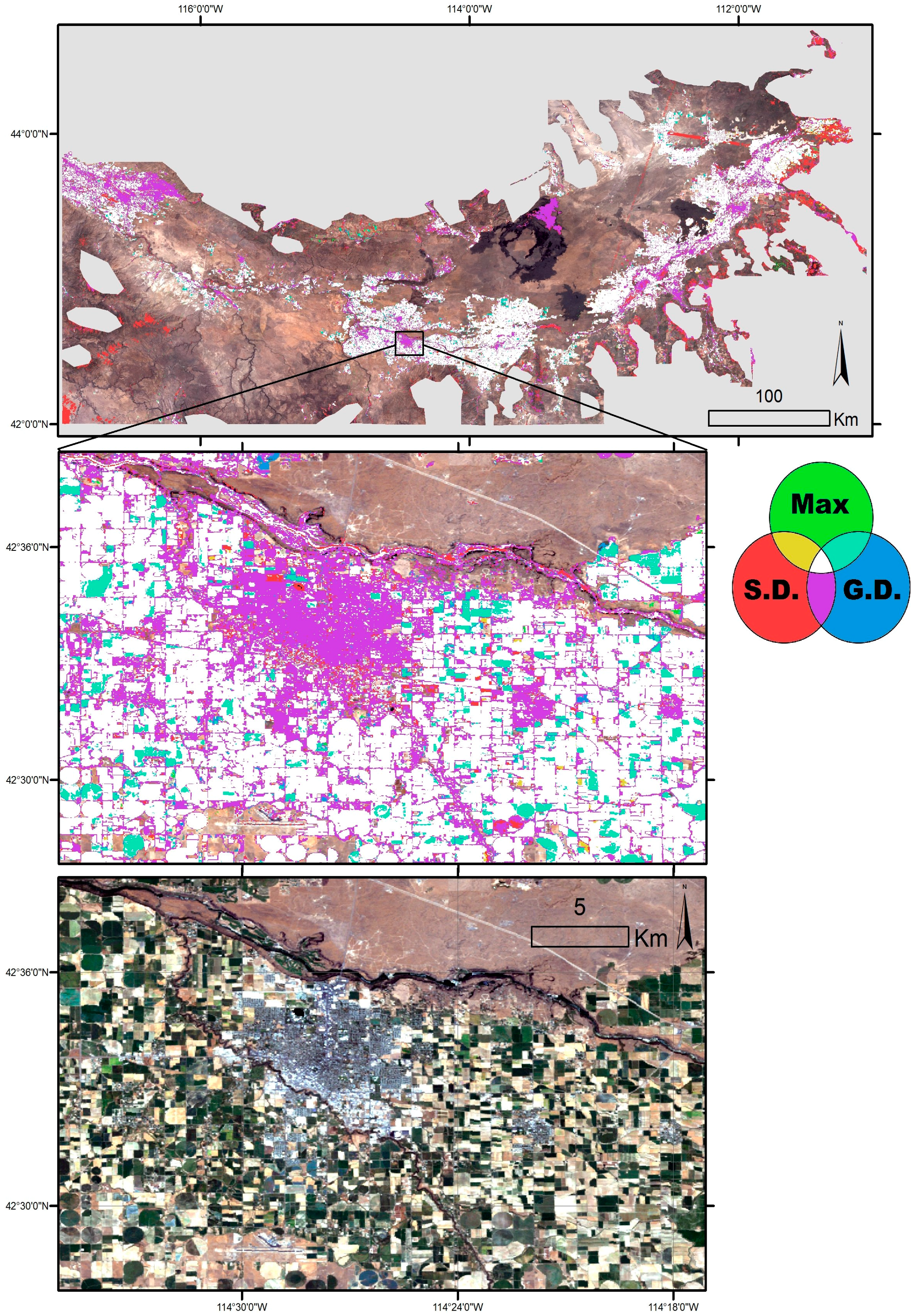
Examination of the multi-temporal trends of NDVI, EVI, and NDMI for our training dataset reveals distinct temporal patterns in elevated index values for irrigated land. The majority of irrigated points exhibit elevated index values following the timing of peak green-up for six composite product cycles (96 days), or approximately three months, prior to declining, likely due to harvest. Other observed trends include: rapidly changing spectra multiple times during the duration of the growing season due to the presence of multi-harvest crops (namely alfalfa); peak response in the late spring and early summer months for spring-planted, irrigated crops; and peak index response during the late summer and early fall months caused by delayed planting. These trends help to explain why the seasonal-maximum algorithm better distinguishes between irrigated agriculture and other areas where vegetation might be green, such as the riparian zone along the Snake River and the urban vegetated environment. Both of these latter scenarios could be considered instances of partial irrigation, characterized by a lesser volume and duration of water use than that for irrigated agriculture. Although the seasonal duration is essentially the same and the contrast between vegetated and non-vegetated land is evident based on all three algorithms, the maximum spectral index value for irrigated land will be greater because vegetation will grow more with additional water use.

The seasonal-maximum algorithm also allows us to accommodate a particular feature of the way that water is allocated to irrigated farms under the state’s system of water rights. Water rights are fulfilled based on the priority (or seniority) of water rights in the region, such that those water rights with an earlier priority date are fulfilled before those with later priority dates. Those fields irrigated with low priority water rights may only have access to water during the beginning of the irrigation season or sporadically thereafter based on available inflows throughout the growing season. In these cases, the seasonal maximum method is best suited to identify areas that were irrigated at any point during the growing season, as this method is more likely to capture short-duration, elevated spectral index values.

The relatively poor performance of the 2002 MODIS NDMI maximum algorithm is due to unmasked clouds, but it highlights one drawback of using the seasonal maximum method: it is more susceptible to errors due to poor masking. A single image during the year containing unmasked clouds, snow, standing water or other extreme values will be the seasonal maximum for that location, and thus will be carried through to the final composite image. These erroneous values would also alter a seasonal average or median image or a smoothed time series, but its impact would be offset by additional correct values and the magnitude of its effect on the final composite would be smaller.

5.1. Sources of Uncertainty

Some sources of uncertainty should be considered. One potential source of error is the influence of precipitation events that temporarily increase vegetative growth and spectral index values in some regions. In non-irrigated agricultural areas, precipitation during the growing season could cause the index values at these areas to be erroneously classified as irrigated. In addition, rain-fed crops tend to maintain elevated index values longer into the growing season relative to other non-agricultural lands, making discrimination between irrigated and non-irrigated areas subtler and leading to larger irrigated area estimates when compared to the USDA Census.

Selection of training/validation data points for this study is likely another source of error. These datasets are limited and the observation points may not be representative of the region as a whole. This is important to consider when evaluating the pixel level accuracy assessments. All the methods performed relatively well at the pixel scale, so small differences in the performance between methods may only represent classification changes at one or two validation points. The data were developed using NAIP imagery, which is simply a one-time image of the land surface, to locate points that appeared to exhibit irrigated and non-irrigated characteristics. Because these images are snapshot in time and land use can change rapidly, it is possible that irrigation was used at other times during the season. It should also be noted that for the initial point validation (using the symmetrical dataset) only points that could be definitively identified as irrigated or non-irrigated based on the NAIP imagery were included. These points may be easier to classify than the landscape as a whole, and could contribute to the relatively high pixel scale accuracy of all of the methods. Having access to a larger dataset of known land-use points has the potential to significantly improve classification accuracy. Individual-level data on land and water use, such as that collected as part of the USDA Census, are typically private, but improved information on field-scale water use would improve the accuracy with which irrigated lands can be mapped. Finally, inclusion of higher-resolution spatial data quantifying annual precipitation amounts and timing may also improve classification accuracies.

5.2. Future Extensions of This Research

Using the Landsat remote sensing dataset from Google Earth Engine to apply our classification algorithm to the full satellite record can allow for accounting of irrigator decision-making over time. A longer data record would support data-driven studies of the impacts of climate change on land-use decision-making. Additional benefits of using the Landsat remote sensing dataset include the increased spatial resolution from MODIS’s 250-m to 30-m. This allows for a more accurate analysis on the sub-MODIS pixel scale, which reduces errors in small-scale plot classification [38]. For example, multiple irrigated and non-irrigated parcels may reside within one 250-m MODIS pixel, leading to a classification error based upon the intensity of irrigation and the resulting influence on the composited NDVI for that pixel. Research has shown that using data at a finer spatial resolution to map irrigated land improves classification accuracy [5]. The downside with Landsat, however, is that the temporal resolution increases to approximately 16 days between each image capture. If insufficient cloud-free images are available, it is challenging to accurately describe the trajectory of NDMI over the growing season and difficult to implement the greenness-duration or seasonal-maximum algorithms. Researchers may thus be forced to accept a tradeoff between spatial resolution and classification accuracy. The decision of which dataset and algorithm(s) to use will depend on the particular research question at hand and the spatial scale at which decision-making processes operate.

Limiting the study region to areas suitable for agriculture is also an important component of this analysis. Forested regions and riparian zones show elevated NDVI and other spectral index values, similar to irrigated areas, meaning they appear as though they are irrigated. Because the influence of riparian zones is limited in our study region, our main focus is on masking out forested areas. The presence of forests poses a significant problem when attempting to quantify irrigated land use at the county scale, likely resulting in an overestimation of irrigated land use. There appear to be distinct patterns in the NDVI curves including the timing of green-up, the slope of the decline in greenness during the growing season, and the timing of rapid NDVI drop-off near the end of the year, likely attributable to the presence of snow or defoliation of undergrowth in inter-canopy spaces. With further exploration of these patterns, a method for removing these regions could be developed.

Lastly, we must discuss the broader applications of our classification method for mapping other semi-arid to arid regions. The developed method relies on region specific training data to calculate each threshold. Since the thresholds are data driven, this method is likely applicable to other regions once a training dataset has been created and could be applied to other types of smoothed time series or composites. Our methods are directly applicable to areas with a “summer dry” climate because they fundamentally rely on a lack of available water for plant consumption during the summer months to identify locations that receive supplemental irrigation water. Because of this assumption, our approaches will be less accurate in areas with “summer wet” climates. It is possible to apply our method to these regions by adjusting the timing and length of the observation window. The required change to the observation period would depend on the timing and length of the growing season along with the timing and magnitude of precipitation. If there is a significant amount of time in which precipitation is low and temperatures are high during the growing season, this method could be applied to map irrigated agricultural land use in areas with “monsoon-driven” semi-arid to arid climates.

6. Conclusions

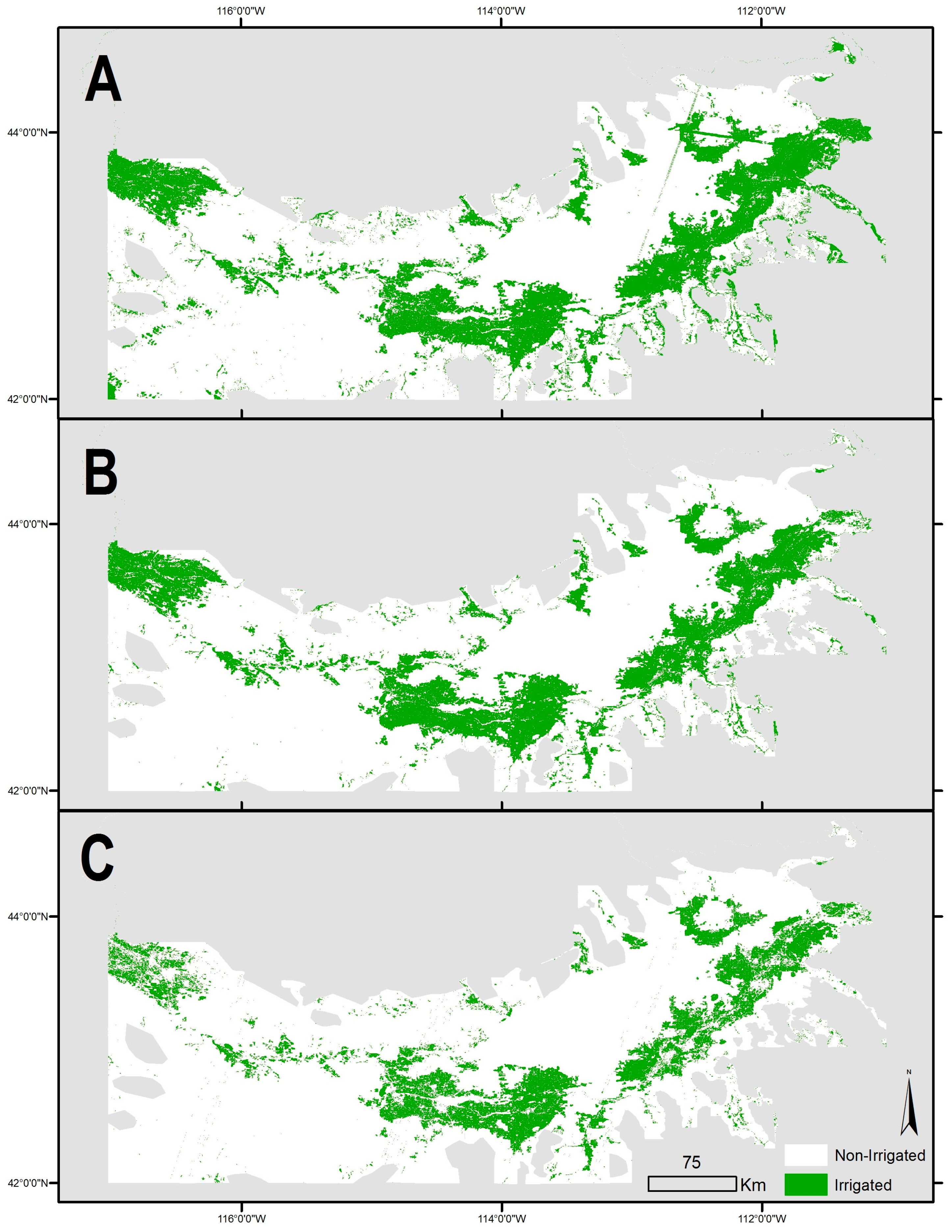
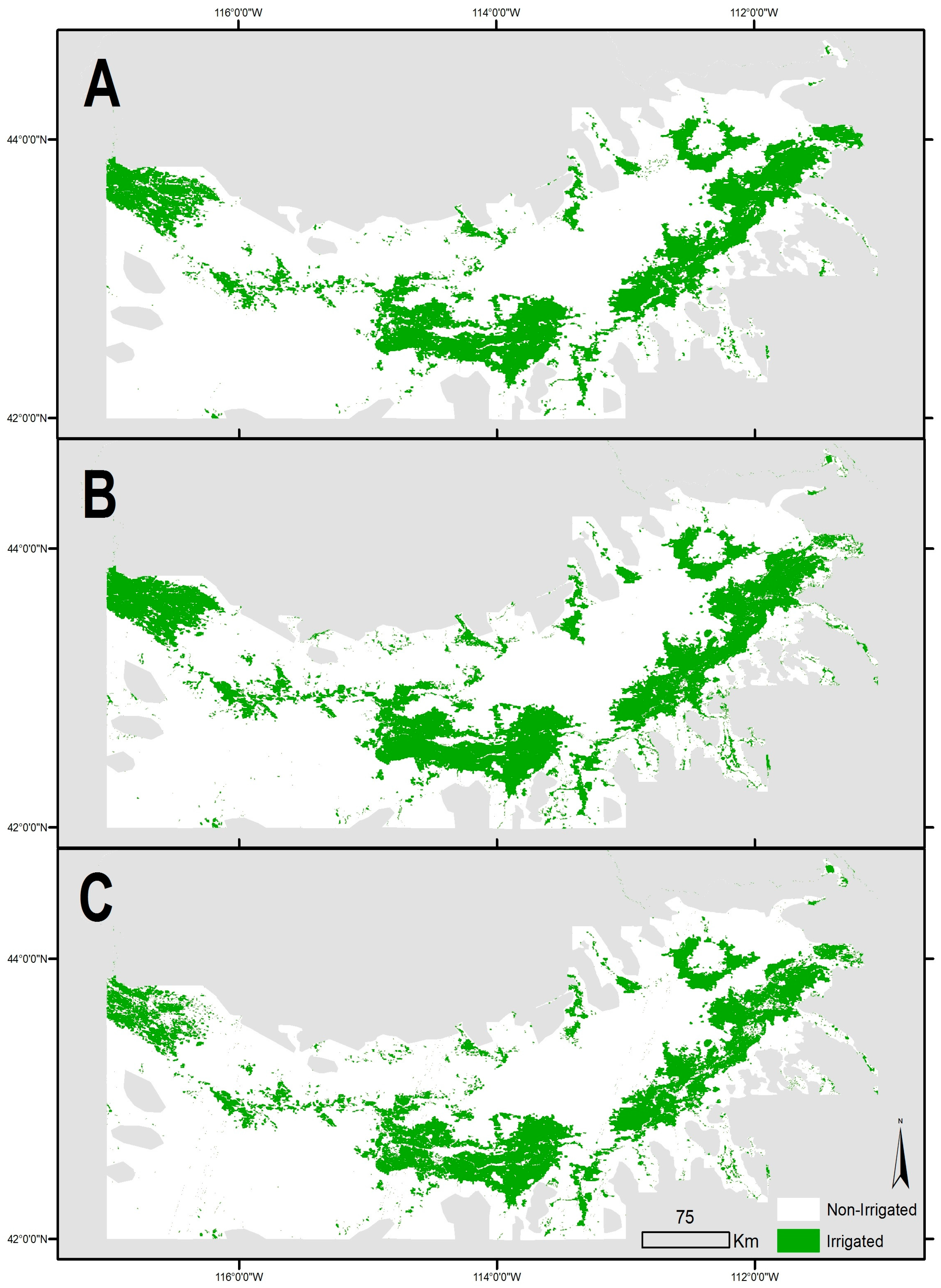
At the regional scale, we demonstrate that the top performing algorithm in terms of classification accuracy is the seasonal-maximum algorithm, primarily due to its out-performance of the other approaches in appropriately classifying lands in riparian and developed areas. While the most accurate method in terms of county scale RMSE and R² is the seasonal maximum of Landsat 5 NDMI, it only marginally outperforms the next best method (Landsat 5, EVI seasonal maximum). Differences in classification accuracy between spectral indices and sensors are fairly modest, but larger differences can be seen between image compositing algorithms. The seasonal maximum algorithm reduces county scale RMSE by an average of 60% over the single-date algorithm, and yields a consistent improvement in classification accuracy across virtually all years and spectral indices. The improved ability of the seasonal-maximum algorithm to classify irrigated and non-irrigated lands at a regional scale is a critical tool for water managers that can support improved predictions of changes in competition for increasingly scarce water resources and provide the information needed to support more efficient water management techniques [5].

Using the seasonal-maximum of spectral vegetation indices, we develop an efficient and computationally inexpensive method for mapping irrigated land use that is broadly applicable to “summer dry” Mediterranean style semi-arid to arid climates. Results show an average percent error reduction when compared to the single-date algorithm of Ozdogan et al. [5]. This is encouraging, given the variability across our study region in terms of topography, precipitation, and temperatures, which represents a significant difference between our analysis and the relatively homogeneous study area in Turkey evaluated by Ozdogan et al. [5].

References

1. Reynolds, J.F.; Smith, D.M.; Lambin, E.F.; Turner, B.L.; Mortimore, M.; Batterbury, S.P.; Downing, T.E.; Dowlatabadi, H.; Fernández, R.J.; Herrick, J.E.; et al. Global desertification: Building a science for dryland development. Science 2007, 316, 847–851. [Google Scholar] [CrossRef] [PubMed]
2. Salem, B. Arid Zone Forestry: A Guide for Field Technicians; Food and Agriculture Organization (FAO): Roma, Italy, 1989. [Google Scholar]
3. Maupin, M.A.; Kenny, J.F.; Hutson, S.S.; Lovelace, J.K.; Barber, N.L.; Linsey, K.S. Estimated Use of Water in the United States in 2010: U.S. Geological Survey Circular 1405; USGS (United States Geological Survey): Reston, VA, USA, 2014.
4. Wardlow, B.D.; Egbert, S.L.; Kastens, J.H. Analysis of time-series MODIS 250 m vegetation index data for crop classification in the US Central Great Plains. Remote Sens. Environ. 2007, 108, 290–310. [Google Scholar] [CrossRef]
5. Ozdogan, M.; Woodcock, C.; Salvucci, G.; Demir, H. Changes in summer irrigated crop area and water use in Southeastern Turkey from 1993 to 2002: Implications for current and future water resources. Water Res. Manag. 2006, 20, 467–488. [Google Scholar] [CrossRef]
6. Ozdogan, M.; Yang, Y.; Allez, G.; Cervantes, C. Remote sensing of irrigated agriculture: Opportunities and challenges. Remote Sens. 2010, 2, 2274–2304. [Google Scholar] [CrossRef]
7. Biggs, T.W.; Thenkabail, P.S.; Gumma, M.K.; Scott, C.A.; Parthasaradhi, G.R.; Turral, H.N. Irrigated area mapping in heterogeneous landscapes with MODIS time series, ground truth and census data, Krishna Basin, India. Int. J. Remote Sens. 2006, 27, 4245–4266. [Google Scholar] [CrossRef]
8. De Fries, R.; Hansen, M.; Townshend, J.R.G.; Sohlberg, R. Global land cover classifications at 8 km spatial resolution: The use of training data derived from Landsat imagery in decision tree classifiers. Int. J. Remote Sens. 1998, 19, 3141–3168. [Google Scholar] [CrossRef]
9. Goward, S.N.; Markham, B.; Dye, D.G.; Dulaney, W.; Yang, J. Normalized difference vegetation index measurements from the Advanced Very High. Resolution Radiometer. Remote Sens. Environ. 1991, 35, 257–277. [Google Scholar] [CrossRef]
10. Justice, C.O.; Townshend, J.R.G.; Holben, B.N.; Tucker, C.J. Analysis of the phenology of global vegetation using meteorological satellite data. Int. J. Remote Sens. 1985, 6, 1271–1318. [Google Scholar] [CrossRef]
11. Myneni, R.B.; Hall, F.G.; Sellers, P.J.; Marshak, A.L. The interpretation of spectral vegetation indexes. IEEE Trans. Geosci. Remote Sens. 1995, 33, 481–486. [Google Scholar] [CrossRef]
12. Nicholson, S.E.; Davenport, M.L.; Malo, A.R. A comparison of the vegetation response to rainfall in the Sahel and East. Africa, using normalized difference vegetation index from NOAA AVHRR. Clim. Chang. 1990, 17, 209–241. [Google Scholar] [CrossRef]
13. Abuzar, M.; McAllister, A.; Morris, M. Classification of seasonal images for monitoring irrigated crops in a salinity-affected area of Australia. Int. J. Remote Sens. 2001, 22, 717–726. [Google Scholar] [CrossRef]
14. Beltran, C.M.; Belmonte, A.C. Irrigated crop area estimation using Landsat TM imagery in La Mancha, Spain. Photogramm. Eng. Remote Sens. 2001, 67, 1177–1184. [Google Scholar]
15. Eckhardt, D.; Verdin, J.; Lyford, G. Automated update of an irrigated lands GIS using SPOT HRV imagery. Photogramm. Eng. Remote Sens. 1990, 56, 1515–1522. [Google Scholar]
16. Kolm, K.E.; Case, H., III. The identification of irrigated crop types and estimation of acreages from Landsat imagery. Photogramm. Eng. Remote Sens. 1984, 50, 1479–1490. [Google Scholar]
17. Thenkabail, P.S.; Schull, M.; Turral, H. Ganges and Indus river basin land use/land cover (LULC) and irrigated area mapping using continuous streams of MODIS data. Remote Sens. Environ. 2005, 95, 317–341. [Google Scholar] [CrossRef]
18. Dheeravath, V.; Thenkabail, P.S.; Chandrakantha, G.; Noojipady, P.; Reddy, G.P.O.; Biradar, C.M.; Gumma, M.K.; Velpuri, M. Irrigated areas of India derived using MODIS 500 m time series for the years 2001–2003. ISPRS J. Photogramm. Remote Sens. 2010, 65, 42–59. [Google Scholar] [CrossRef]
19. Wardlow, B.D.; Egbert, S.L. Large-area crop mapping using time-series MODIS 250 m NDVI data: An assessment for the US Central Great Plains. Remote Sens. Environ. 2008, 112, 1096–1116. [Google Scholar] [CrossRef]
20. Huete, A.; Didan, K.; Miura, T.; Rodriguez, E.P.; Gao, X.; Ferreira, L.G. Overview of the radiometric and biophysical performance of the MODIS vegetation indices. Remote Sens. Environ. 2002, 83, 195–213. [Google Scholar] [CrossRef]
21. Draeger, W.C. Monitoring Irrigated Land Acreage Using Landsat Imagery: An Application Example; USGS (United States Geological Survey): Reston, VA, USA, 1977.
22. Thiruvengadachari, S. Satellite sensing of irrigation patterns in semiarid areas: An Indian study [Tamil Nadu State, India]. Photogramm. Eng. Remote Sens. 1981, 47, 1493–1499. [Google Scholar]
23. Ruffner, J.A.; Bair, F.E. National Oceanic and Atmospheric Administration Narrative Summaries, Tables and Maps for Each State with Overview of State Climatologist Programs; Gale Research Company: Farmington Hills, MI, USA, 1985. [Google Scholar]
24. USGS (United States Geological Survey). Water Use Data for Idaho; USGS (United States Geological Survey): Reston, VA, USA, 2016.
25. Kenny, J.F.; Barber, N.L.; Hutson, S.S.; Linsey, K.S.; Lovelace, J.K.; Maupin, M.A. Estimated Use of Water in the United States in 2005; USGS (United States Geological Survey): Reston, VA, USA, 2009.
26. Karl, T.R. Global Climate Change Impacts in the United States; Cambridge University Press: Cambridge, UK, 2009. [Google Scholar]
27. Kunkel, M.L.; Pierce, J.L. Reconstructing snowmelt in Idaho’s watershed using historic streamflow records. Clim. Chang. 2010, 98, 155–176. [Google Scholar] [CrossRef]
28. Zhu, Z.; Wang, S.; Woodcock, C.E. Improvement and expansion of the Fmask algorithm: Cloud, cloud shadow, and snow detection for Landsats 4–7, 8, and Sentinel 2 images. Remote Sens. Environ. 2015, 159, 269–277. [Google Scholar] [CrossRef]
29. Tucker, C.J. Red and photographic infrared linear combinations for monitoring vegetation. Remote Sens. Environ. 1979, 8, 127–150. [Google Scholar] [CrossRef]
30. Jiang, Z.; Huete, A.R.; Didan, K.; Miura, T. Development of a two-band enhanced vegetation index without a blue band. Remote Sens. Environ. 2008, 112, 3833–3845. [Google Scholar] [CrossRef]
31. Land Processes Distributed Active Archive Center. Available online: https://lpdaac.usgs.gov/ (accessed on 3 March 2017).
32. Gao, B.C. NDWI—A normalized difference water index for remote sensing of vegetation liquid water from space. Remote Sens. Environm. 1996, 58, 257–266. [Google Scholar] [CrossRef]
33. National Oceanic and Atmospheric Administration. Nws_Precip_Wateryear2date_Normal_Shape_20151001.shp; NOAA: Silver Spring, MD, USA, 2016.
34. IDWR. Water Right: Places of Use; IDWR: Boise, ID, USA, 2015.
35. Cobourn, K.M. Externalities and simultaneity in surface water-groundwater systems: Challenges for water rights institutions. Am. J. Agric. Econ. 2015, 97, 786–808. [Google Scholar] [CrossRef]
36. Ghosh, S.; Cobourn, K.M.; Elbakidze, L. Water banking, conjunctive administration, and drought: The interaction of water markets and prior appropriation in southeastern Idaho. Water Res. Res. 2014, 50, 6927–6949. [Google Scholar] [CrossRef]
37. National Land Cover Database 2011 (NLCD 2011). Available online: https://www.mrlc.gov/nlcd2011.php (accessed on 3 March 2017).
38. Ozdogan, M.; Woodcock, C.E. Resolution dependent errors in remote sensing of cultivated areas. Remote Sens. Environ. 2006, 103, 203–217. [Google Scholar] [CrossRef]
Figure 1. Map of the Snake River Plain (SRP). The Study area consists of the counties containing the SRP with large forested areas removed. Counties in the East Snake Plain are shown in a darker red than those in the west.
Remotesensing 09 00546 g001
Figure 2. (Top) Irrigated and non-irrigated control points, overlain on top of 2007 Landsat 5 imagery for the study region. (Bottom) Enlarged section to illustrate irrigated and non-irrigated areas for several control points.
Remotesensing 09 00546 g002
Figure 3. Diagram of example irrigated and non-irrigated Normalized Difference Vegetation Index (NDVI) curves with metrics used for image classification noted. NDVI is shown; Enhanced Vegetation Index (EVI) and Normalized Difference Moisture Index (NDMI) are similar.
Remotesensing 09 00546 g003
Figure 4. The 2007 irrigated areas classified using Landsat 5 NDMI for the three algorithms: (A) single date algorithm; (B) greenness duration algorithm; and (C) seasonal-maximum algorithm. Non-irrigated areas are shown in white, irrigated areas are green and masked areas outside the study region are grey.
Remotesensing 09 00546 g004
Figure 5. A comparison of the seasonal maximum (Max), single date (SD), and greenness duration (GD) algorithm performance using the year-dataset-spectral index combination 2007-Landsat-NDMI. White areas indicate locations where all algorithms agree that the pixel is irrigated; transparent areas are those that all algorithms agree are non-irrigated. Note the misclassification of urban areas from the SD and GD algorithm shown in purple in the inset image of Twin Falls, ID.
Remotesensing 09 00546 g005