Monitoring the Arctic Seas: How Satellite Altimetry Can Be Used to Detect Open Water in Sea-Ice Regions


Deutsches Geodätisches Forschungsinstitut, Technische Universität München, Arcisstraße 21, 80333 Munich, Germany
*
Author to whom correspondence should be addressed.
Remote Sens. 2017, 9(6), 551; https://doi.org/10.3390/rs9060551
Submission received: 24 February 2017
/
Revised: 23 May 2017
/
Accepted: 29 May 2017
/
Published: 1 June 2017
(This article belongs to the Special Issue Satellite Altimetry for Earth Sciences)
Abstract
:Open water areas surrounded by sea ice significantly influence the ocean-ice-atmosphere interaction and contribute to Arctic climate change. Satellite altimetry can detect these ice openings and enables one to estimate sea surface heights and further altimetry data derived products. This study introduces an innovative, unsupervised classification approach for detecting open water areas in the Greenland Sea based on high-frequency data from Envisat and SARAL. Altimetry radar echoes, also called waveforms, are analyzed regarding different surface conditions. Six waveform features are defined to cluster radar echoes into different groups indicating open water and sea ice waveforms. Therefore, the partitional clustering algorithm K-medoids and the memory-based classification method K-nearest neighbor are employed, yielding an internal misclassification error of about 2%. A quantitative comparison with several SAR images reveals a consistency rate of 76.9% for SARAL and 70.7% for Envisat. These numbers strongly depend on the quality of the SAR images and the time lag between the measurements of both techniques. For a few examples, a consistency rate of more than 90% and a true water detection rate of 94% can be demonstrated. The innovative classification procedure can be used to detect water areas with different spatial extents and can be applied to all available pulse-limited altimetry datasets.
1. Introduction
The Arctic Ocean, including its peripheral seas, e.g., the Greenland Sea, is considered one of the most important components of the Earth’s climate system [1]. In particular, these areas show strong responses to global warming and may affect climate conditions globally, for example, by changing the oceanic thermohaline circulation. The north polar regions are crucial contributors to the global ocean current system by carrying cold and fresh water southwards. Most of the Arctic Ocean is covered by varying extents of sea ice with open water areas and floes with different spatial extents as well as fully closed ice surfaces. The seasonal fluctuations of ice covers significantly impacts the atmosphere-ocean interaction (e.g., ice-albedo). While a closed sea ice cover prevents the ocean from heat emission, openings in the ice lead to a warming of the first atmospheric layers.
The evolution of sea ice is strongly influenced by sea surface temperature, wind, waves and ocean currents [1]. During recent decades, increasing sea surface temperatures and an enhanced warm water inflow in the Arctic Ocean resulted in decreased sea ice extent and volume [2,3]. Additionally, the Greenland ice sheet experienced strong environmental changes due to an increasing mass loss enhancing melt water influx into the Arctic Ocean [4].
The monitoring of the changing north polar ocean conditions, especially in the Greenland Sea, allows investigating interconnections between land, ocean, and atmospheric processes as well as their climate forcing. Today, remote sensing systems provide a large set of different sensors for monitoring the polar regions. Radar satellite altimetry is able to provide quantitative information about sea surface heights, significant wave heights, and dynamic ocean topography [5,6]. However, in order to derive reliable altimetry products, a careful selection of measurements from open water areas is necessary. By analyzing the radar return signal of the altimeter, the so-called waveform, information about the reflecting surface can be derived. This allows the classification of waveforms in water- and sea ice-returns and the detection of open water areas in sea ice regions. For example, calm open water areas within the footprint cause a very single-peak shape. With an along-track resolution of less than a kilometer using high-frequency data, conventional satellite altimetry missions (such as Envisat and SARAL) are able to detect small open water areas that might be missed by imaging Synthetic Aperture Radar (SAR) satellite missions (Sentinel-1A/B, Radarsat-1/2, etc) in case a high-resolution acquisition mode is not available. Additionally, small water areas have insufficient backscatter properties to be mapped by passive microwave satellite missions (e.g., Special Sensor Microwave Imager (SSM/I) and SSM/I Sounder (SSM/IS)). However, altimeter radar echoes reflected from non-uniform scatterers, like sea ice regions, are challenging to interpret because the large surface footprint of several kilometers usually covers several ice types.
The first studies dealing with satellite altimetry in sea ice regions were published in 1980 by Dwyer and Godin [7] and in 1992 by Fetterer et al. [8]. After the launch of the ESA satellites ERS-1 and ERS-2, covering high latitudes in a repeat orbit, further studies were conducted by Laxon [5] and Laxon et al. [9]. They analyzed the potential of ERS-1 sea ice monitoring and the interannual variability of sea ice thickness by employing ERS-1 and ERS-2 altimetry data. Furthermore, Peacock [10] provides a first sea surface height determination in the Arctic ocean. In recent years, several sea ice applications have been explored e.g., the detection of openings in the ice. Connor et al. [11] applied a peakiness parameter, defined by Peacock [10] in order to detect small open water bodies in the sea ice cover using high-frequency data of Envisat. Zakharova et al. [12] continues with the development of a lead detection algorithm by using the Centre National d’ Études Spatiales (CNES) and Indian Space Research Organisation (ISRO) satellite SARAL and maximum power threshold. Currently, all pulse-limited altimetry-based approaches for detecting water returns in sea ice regions use thresholds for different parameters. This has the disadvantage that the thresholds have to be set manually and individually for every altimetry mission. Furthermore, a deep knowledge about the different scatter characteristics in sea ice regions is required. Besides Zygmuntowska et al. [13] developed another approach using the waveforms shape for classifying airborne SAR altimeter echoes over the Arctic sea ice in a supervised way.
The present study proposes a new strategy to detect open water areas based on an unsupervised classification of high-frequency altimetry radar echoes. The approach is able to detect water domains with different spatial extents and can be easily applied without any deeper knowledge about surface-dependent backscatter characteristics. The method is applicable to all available pulse-limited altimeter data and is independent of mission-specific radar frequencies and characteristics. Furthermore, the results are compared to processed SAR images using the method described in [14] to obtain quantitative information about the classification performance.
The present paper is structured into three main parts. First, the study area and the applied datasets are introduced. Section 3 presents the method and processing procedure as well as the comparison process of the obtained results. Section 4 presents the classification results and provides evidence of the classification performance. At first, quantitative information considering the entire available validation dataset (Section 4.1) is derived before some visual comparisons between the SAR images and the altimetry overflights are provided. The paper finishes with a conclusion and an outlook to future research.
2. Study Area and Data Sets
This section provides an introduction to the study area and the different remote sensing datasets used for classification and validation.
2.1. Greenland Sea and Fram Strait
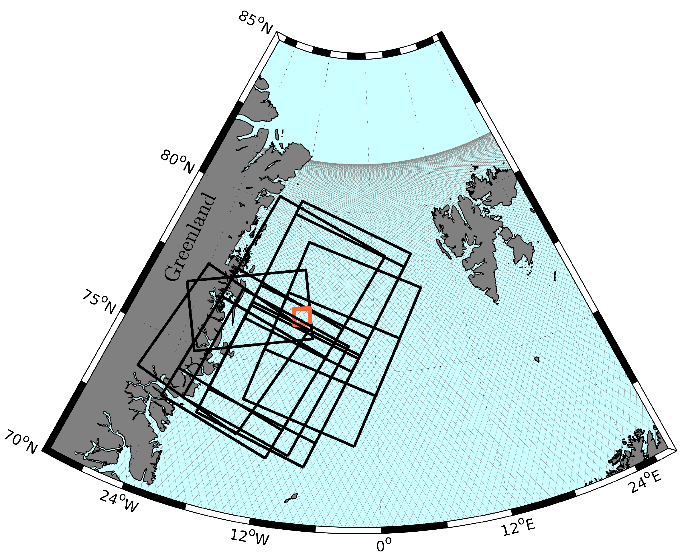
The study area ranges from N to N in latitude and from the north-east coast of Greenland to E in longitude and covers the Greenland Sea and the Fram Strait (see Figure 1 and Figure 2). The Greenland Sea belongs to the peripheral seas of the Arctic ocean. It connects the Fram Strait in the north, a narrow passage between north-east Greenland and Svalbard, with the Norwegian Sea as well as the Iceland Sea in the south. This area is affected by the East Greenland Current (EGC), which transports more than 90% of fragmented sea ice from the Arctic Ocean through the Fram Strait southwards [15]. Therefore, the EGC represents the main and most important freshwater outlet of the Arctic Ocean. According to Serreze and Barry [16] the Greenland Sea and the region of the Fram Strait is strongly influenced by rapid atmospheric and changing sea ice conditions as well as comparatively fast ocean currents with a mean velocity of 20–30 cm/s [17] and maxima up to 80 cm/s [18]. The sea ice state reaches from a nearly closed sea ice cover, showing straight lined and circular shaped open water bodies, leads and polynyas, up to individual ice floes ranging from a few meters to kilometers in diameter [16]. Applying open water detection to the Greenland Sea and the Fram Strait offers one the chance to sensitize the unsupervised classification method for a various number of different sea ice and ocean conditions.
2.2. Radar Altimetry Data
In the present investigation, the high-frequency radar altimetry data of the ESA satellite Envisat and the CNES/ISRO altimetry satellite SARAL are used. Data of the missions Jason-1, Jason-2 and Jason-3 are disregarded due to their low orbit inclination (about ) not covering the Greenland Sea and Fram Strait.
Envisat and SARAL carry pulse-limited radar altimeters and are placed on the same 35 day repeat-orbit covering polar areas up to geographical latitude. Envisat was launched in March 2002 and orbits the Earth at an altitude of nearly 800 km. In October 2010, Envisat left the repeat-orbit and started to drift until in May 2012, the ESA mission was decommissioned after an unexpected signal loss. SARAL was placed in orbit in February 2013 and is still active even though in July 2016, the satellite started its drifting orbit phase without fix repeat period.
All computations and methodologies used in this study are based on official high-frequency Sensor Geophysical Data Record (SGDR) v2.1 dataset of Envisat’s radar altimeter (RA-2) and the SGDR-T dataset of the AltiKa radar altimeter mounted on SARAL. In case of SARAL, data until July 2016 and in case of Envisat, data until the end of the mission are used. In this study, waveforms observed in the Greenland Sea and Fram Strait (see Section 2.1) are employed in the classification process. In order to calculate the altimeter backscatter values, different features stored in the SGDR dataset, for example, atmospheric attenuation and instrumental corrections (e.g., sigma naught calibration factor) are additionally used.
The two satellite missions differ mainly in the emitted radar bandwidth, the pulse repetition frequency and the footprint size of the illuminating area onto the surface. RA-2 emits -band signals with an repetition frequency of 1800 pulses per second, covering an nominal elliptic area of approximately up to 10 km diameter [11] depending on the surface conditions. Before transmitting to earth, the waveforms are sampled to 18 Hz by the on-board processing. AltiKa works in the -band, with a repetition frequency of 4 kHz, generates 40 Hz averaged waveforms and has half the antenna aperture of Envisat. This leads to a smaller footprint size up to 8 km diameter and an improved spatial resolution [19]. Beside instrumental influences, the waveform’s shape is mainly affected by various surface characteristics. Detailed explanations referring to the representation of the varying waveform’s shape can be found in Section 3.1.
2.3. Imaging Synthetic Aperture Radar (SAR) Data
A possible source for validating the classification results is the usage of imaging synthetic aperture radar (SAR) data. Beside the altimeter satellites, several multispectral and SAR imaging satellite missions regularly provide snapshots of periodically changing ocean conditions. In contrast to multispectral sensors, working mostly in the visible and infrared spectrum, SAR sensors are unaffected by cloudiness and lighting conditions, which makes it easier to identify appropriate scenes. However, SAR sensors are side-looking instruments, which can cause a shadowing of very flat and smooth surface structures (e.g., leads or polynyas) due to interjacent higher topography (e.g., ice floes, ridges). Additionally, the recorded backscatter values do not only depend on the surface characteristics (e.g., roughness) but also on the incidence angle of the reflected radar waves, which makes it more complex to provide information about different surface types. Furthermore, it has to be mentioned that most SAR satellites are placed on sun-synchronous orbits, which allows for a uniform capture of ice state but limits the minimum time lag between the acquisition dates of the SAR images and the altimetry measurements of Envisat and SARAL also using sun-synchronous orbits.
Aiming at a small time lag between SAR images and satellite altimetry, wide swath data are qualified best since these images cover a spatially extended area with medium pixel spacing. For this investigation, SAR images of the JAXA Advanced Land Observing Satellite (ALOS) [20], MDA’s Radarsat-2 [21] and ESA’s Sentinel-1A (S-1A) [22] are used. The Envisat classification results are compared with ALOS PALSAR Level 1.5 Wide Beam (WB) images offered by the Alaska Satellite Facility (ASF) DAAC and with Radarsat-2 (R-2) Scan SAR Mode data provided by ESA. The SARAL classification outcomes are compared with Level-1, S-1A extra wide swath mode data. S-1A images are made available through the ESA/Copernicus Sentinel Data Hub. Specifications, temporal availability in the target region, and information about the used imaging SAR products are listed in Table 1. To distinguish between open water pixels, appearing in near black, and sea ice pixels, appearing in bright gray, HH-polarized images are used. For more information regarding SAR polarization and the influence of different surface scattering see Dierking W. [23] and Jackson et al. [24].
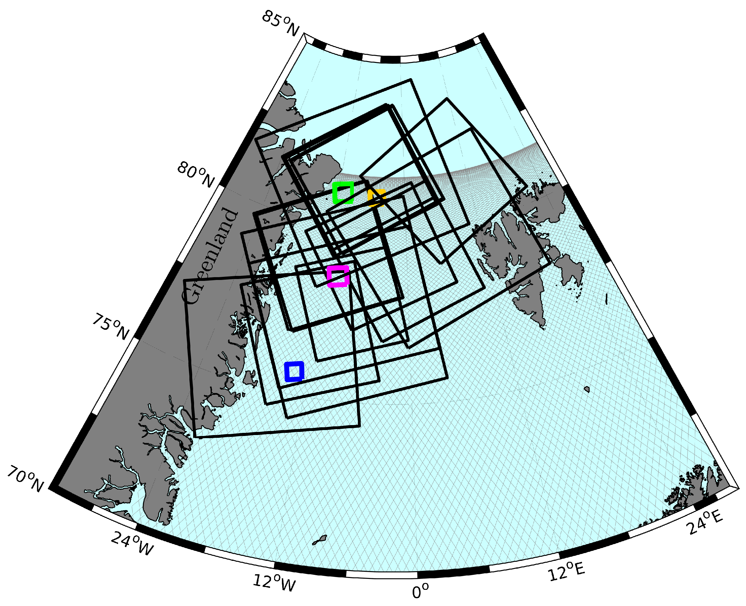
In order to ensure similar sea ice conditions and allow for an unbiased comparison between SAR and altimetry, only images with a time lag less than about 3.5 h, with respect to the altimetry crossings, are used. The comparison is based on 16 grayscaled SAR images during the lifetime of Envisat and 19 images for SARAL. The SAR data are selected from different epochs considering a varying sea surface state with a focus on periods with various sea ice coverage. Figure 1 and Figure 2 display the locations of all used SAR images. The scenes are mainly located in the Fram Strait and near the north-east coast of Greenland. Table 2 and Table 3 list sensor and temporal information for all conducted comparison pairs. Two of the R-2 images are used for multiple satellite overflights. In the case of SARAL classification, it has to be mentioned that, due to sun-synchronous orbits and fixed revisit times of Sentinel-1A and SARAL, it is not possible to find suitable pairs for comparison that show good spatio-temporal coverage with a time gap smaller than 2 h 40 min during the study period.
2.4. Sea Ice Data
Polar sea areas are affected by moving sea ice due to the influences of wind and ocean currents [16]. This results in a rapid change and high diversity of the sea surface conditions. To reach a realistic comparison of altimetry results and SAR images, the compensation for sea ice motion within the time interval between the two observation sets is required. For this purpose, daily ice vector velocity fields are exploited within the validation process. Therefore, the “Polar Pathfinder Daily 25 km EASE-Grid Sea Ice Motion Vectors, Version 3” of the National Snow and Ice Data Center (NSIDC) are employed [25]. This dataset contains zonal and meridional sea ice velocity observations of active and passive sensors as well as in situ measurements interpolated to a 25 km spacing grid referring to an azimuthal equal area map projection. This dataset covers the entire altimetry era until the end of May 2015.
The sea ice velocity data are used to shift the SAR image, respectively, the image pixel coordinates, assuming an averaged ice motion (direction and velocity) over the time interval between the altimetry measurement and the SAR image. For this purpose, only homogeneous data represented by small standard deviations in direction and velocity inside a predefined box ( km) around the altimetry track are selected to compute a mean displacement vector. Sea ice velocity vectors located close to the coastlines (within 25 km) are eliminated due to erroneous ice observations [25].
The comparison is performed only in areas affected by sea ice to suppress the influence of falsely detected SAR ice pixels caused by diffuse scattering behavior due to rough swell in the open ocean. Therefore, daily “Sea Ice Concentrations from Nimbus-7 SMMR and DMSP SSM/I-SSM/IS Passive Microwave Data, Version 1” of the NSIDC [26] with a spatial resolution of 25 km × 25 km are interpolated to the altimetry high-frequency data. Observations outside the ice edge without sea ice are excluded from the comparison process.
3. Methods
This study is based on an unsupervised classification process of altimetry waveforms. Unsupervised classification algorithms group unassigned data into a predefined number of classes without any background information about the data and their sources using only “natural“ and hidden intra-cluster similarities [27]. The classification is performed based on a set of features characterizing the input data. In contrast, supervised classification is based on a-priori information of a well known or labeled dataset to classify and assign the observations [28]. Examples for unsupervised classification methods are artificial neural networks (e.g., Self-Organizing Maps [29]) or partitional clustering algorithms (e.g., K-means and K-medoids [30,31]). In the present investigation, a partitional cluster algorithm, K-medoids, is used for separating a set of unlabeled waveform data into clusters indicating different waveform properties. Therefore, features have to be defined describing various waveform characteristics. Based on the clustering results, K-nearest-neighbor is applied to assign unclassified waveform data.
In this section, at first, features for describing the various waveform shapes and their characteristics are specified and explained. This is followed by the description of the methodical background of the clustering and classification process. The last part of Section 3 presents the validation approach for the classification procedure. The presented methods are applied independently to Envisat and SARAL.
3.1. Waveform Features
The shape of altimetry waveforms strongly depends on the surface characteristics within the altimeter footprint. Figure 3 shows Envisat/RA-2 and SARAL/AltiKa radar pulses reflected by ocean, leads, and sea ice. Major differences can be detected in the power magnitude and the number and shape of the signal peaks. Leads produce very narrow and peaky waveforms due to the specular scattering of calm and flat water. In contrast, radar pulses originating from ocean or sea ice surfaces are influenced by waves or interlaced and piled ice floes, respectively, leading to multi peaks and wider, noisier shapes.
In order to characterize a waveform and identify the main evocative surface scatterer, a number of waveform features are defined. The computed values constitute a waveform feature space that provides the input for the clustering and classification process. To increase the efficiency of the algorithm and to get a reliable open water detection, the selected features should fulfill the following conditions:
- The features should characterize different waveform types.
- The selected features should be stand alone and without linear dependence and major correlations among each other.
- The feature space should be adaptable to any altimetry waveform.
- All features should exhibit the same order of magnitude for equal weighting among each other.
In the present investigation, six features are defined to describe the waveforms mainly focusing on the reflected radar pulse shape (width) and the recorded power intensity. These features are applicable for each pulse-limited altimeter waveform, i.e., for Envisat as well as for SARAL.
- Waveform maximum (Wm)The waveform height is described by the maximal power of the returning radar pulse . It provides information about the backscatter of calm or rough surface conditions. To compute for Envisat as well as SARAL, the maximum waveform power and mission specific rectifications are applied by using instrumental and atmospheric corrections from the provided datasets (see Section 2.2).
- Trailing edge decline (Ted)The trailing edge decline is computed by fitting an exponential function, considering an exponential decay of AltiKa waveforms, from the waveform power maximum to the last bin. The estimated decay rate is used to characterize the decline of the trailing edge after the maximum.
- Waveform noise (Wn)This feature quantifies the trailing edge scattering. It is computed as median absolute deviations of the trailing edge fitting (see Ted) residuals. This parameter is very small for single peak waveforms (leads) and moderate for oceans.
- Waveform width (Ww)The number of bins where the power is equal to zero provides information about the waveform’s width.
- Leading edge slope (Les)The leading edge slope is obtained by subtracting the first bin position containing more than 30% of the power maximum from the bin position of the maximum power. The difference provides relative information about the width and steepness of the leading edge independent of the absolute position of the leading edge, i.e., the range.
- Trailing edge slope (Tes)In contrast to the leading edge slope, the trailing edge slope is obtained by subtracting the last bin position containing more than 30% of the maximum from the bin position of the maximum power. This difference provides similar information to Ted in the case of single-peak waveforms but supports the identification of strong specular peaks in front of an ocean-like trailing edge.
The selected features in the present investigation show a varying order of magnitudes, which results in an irregular weighting in the clustering algorithm. In order to comply with condition 4 (see above) a standardization has to be processed. Before conducting the unsupervised classification procedure, the features are reduced by subtracting their average and divided by their standard deviation (standard-score).
The features are calculated for RA-2 and AltiKa waveforms in the same way. In the case of SARAL, the maximum power is limited to 1250 counts. Power counts above this limit are not recorded due to too high backscatter values that cannot be resolved by the tracking window [12]. The waveforms are cut without a clear maximum peak in the radar echo, which makes it impossible to compute all features (e.g., leading edge slope) and to constitute the complete feature space. These waveforms, which are not flagged in the SGDR dataset, are skipped from the further classification process. Furthermore, all waveforms are neglected, for which no reliable computation of the defined features is possible (e.g., if trailing edge fitting is impossible with 95% confidence).
3.2. Clustering
Within the clustering process a representative subset of all waveforms from a single mission will be used to define waveform groups, so-called clusters, that will later be used to also classify all remaining observations. In a first step, this reference model has to be created. For this purpose, a set of several waveforms, containing a majority of all possible scatter types, has to be selected. To this end, waveform data covering an area in the central Greenland Sea within bounds of W/E longitude and N/N latitude are used. To cover as many sea ice types as possible, the epoch is selected at the beginning of the melting period in early summer from April to May [32]. For Envisat, Cycle 57 (2007, containing about 307,000 waveforms), and for SARAL, Cycle 12 (2014, ca. 670,000 waveforms) are selected.
To group the reference data, a K-medoids cluster algorithm is implemented that clusters unsupervised data into K clusters. K-medoids performs a distance minimization between the features and the most centrally located feature (medoids) based on the feature space itself. Thereby, K-medoids is more robust to outliers and noise in contrast to K-means, which tries iteratively to estimate an optimal partition of unlabeled data by minimizing the distances between the coordinates of a mean cluster center (centeroids) and the features. However, in contrast to K-medoids, K-means integrates every value of the feature space into the arithmetic average [27].
At first, K-medoids randomly chooses K medoids of the feature space and computes the distances to every feature. In the next steps, the algorithm rearranges every single feature until there is no motion within the K clusters and the minimal distances to the medoids are found. However, the clustering result depends on the initial randomly chosen medoids. This is why the algorithm is repeated several times and the best solution is selected by analyzing the final sum of all distances within the clusters. This leads to high computational efforts by employing large input datasets, but it is considerable that the clustering has to be performed just once per altimetry mission. To reduce the computation times, the algorithm examines only a random sample of cluster members during each medoids updating step. The size of the sample is set by default to 0.1% of the total number of data points. The iteration terminates if the medoids are stabilized.
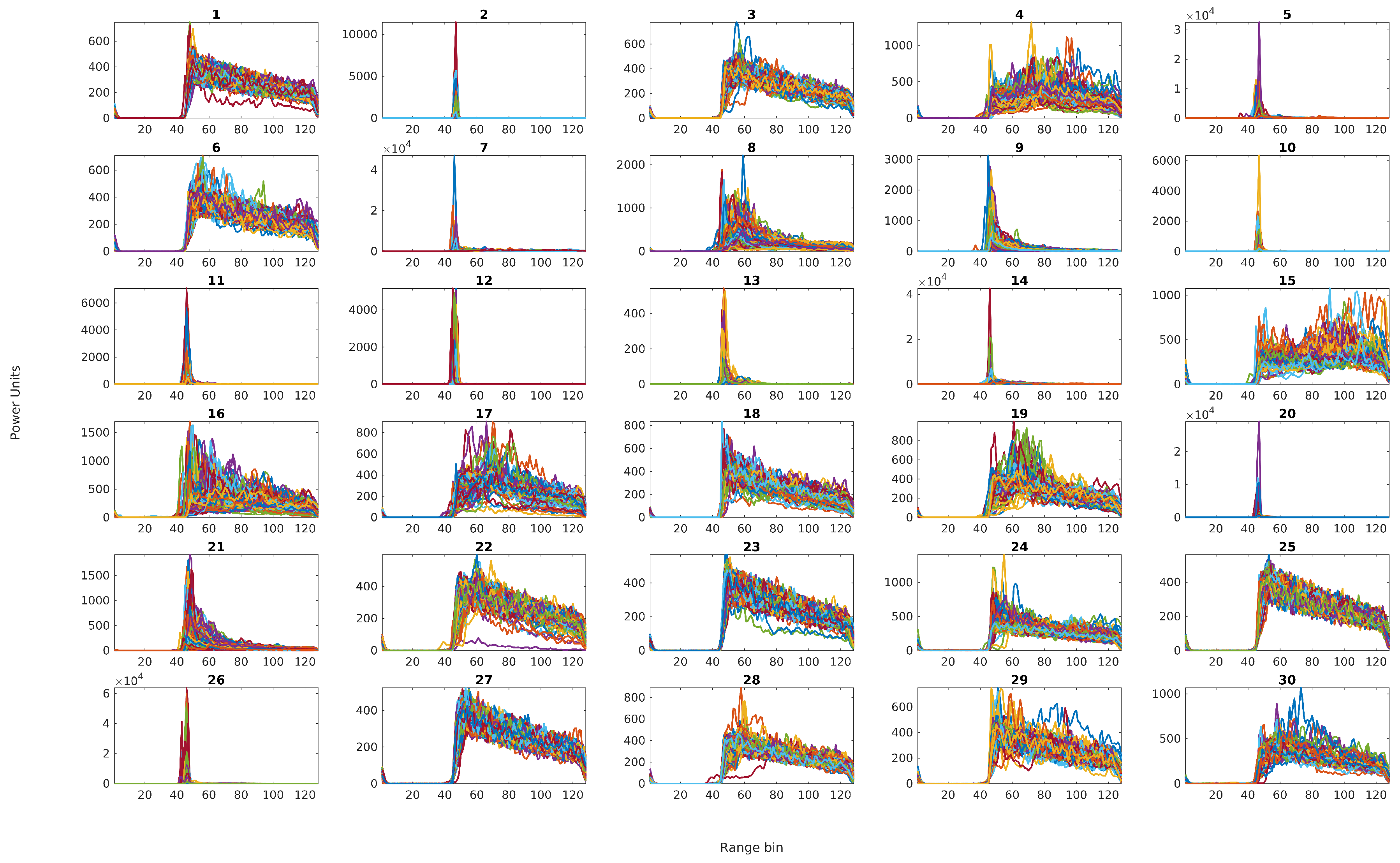
Partition clustering algorithms require an initialization of the number of clusters K. In the present investigation, K is chosen empirically after several test runs by evaluating the best segmentation results [31]. Indicators for defining an appropriate K are, for example, the analysis of the sum of all distances within the clusters and, additionally, a visual analysis of all clusters. In order to obtain a clear partitioning of waveforms, it is useful to set K larger than the desired number of the three surface types, the present investigation is looking for, namely, calm open water, ocean or sea ice conditions. Figure 4 shows the clustering for 30 classes based on derived waveform features of about 307,000 Envisat waveforms (the clustering results for SARAL waveforms can be found in the Supplementary section, Figure S1). The displacements between the points and the medoids are computed using Euclidean distances.
After running K-medoids, each cluster has to be assigned to one surface condition. The 30 clusters need to be manually condensed to three main classes indicating ocean, sea ice, and lead/polynya returns. This is done based on the feature statistic per cluster (see Figure 5) and knowledge on the physical backscattering behavior of different surfaces. It is well known that radar returns from dominant scatterers (i.e., a lead with a calm, mirror-like surface) cause single-peak waveforms with high power and narrow shape. Radar echoes nearly entirely reflected by sea-ice show a more diffuse scattering, weak power and no clear peaks. Using these relationships and transferring them to the cluster statistics enable a nearly unambiguous assignment. However, questionable clusters with ambiguous feature properties remain and are labeled as ”undefined“.
Figure 5 indicates the cluster assignment by different colors. Lead and polynya returns (clusters 2, 10–12, 20, and 26) are characterized by a very narrow and peaky shape and high maximum power values. In contrast, ocean returns (clusters 1, 3, 6, 18, 22, 23, 25, 27–29) are wider and show a greater trailing edge decay. Waveforms belonging to the ice class (clusters 5, 7–9, 13, 14, 16, 21, 24, and 30) are between these two groups. They are defined by a smaller trailing edge decay and slope as well as bigger power values than ocean returns. However, there are clusters (4, 15, 17, and 19), that cannot clearly be assigned to one surface type. As an example, cluster 19 shows an ocean like behavior, but is characterized by an indistinct leading edge as well as a steeper ice-like trailing edge. Undefined waveform classes show, apart from more noise in the cluster itself, no clear signature or trend to the underlying feature space or to the three main surface classes.
3.3. Classification
The waveform model created by the clustering (Section 3.2) can now be used to classify all waveforms. For this purpose the K-Nearest Neighbor (K-NN) classifier is employed. In general, K-NN belongs to the memory-based classifiers and does not require a stochastic model [28]. Basically, K-NN searches for the closest distance between a query point and a given input model. Similar to the K-medoids algorithm, the K-NN uses the euclidean distance. However, K has a completely different meaning than in the K-medoids algorithm. The K is now defined as the number of neighbors used for the classification. The cluster assignment of a specific waveform is done based on the majority of clusters of these K nearest neighbors. K must be set before the classification process starts.
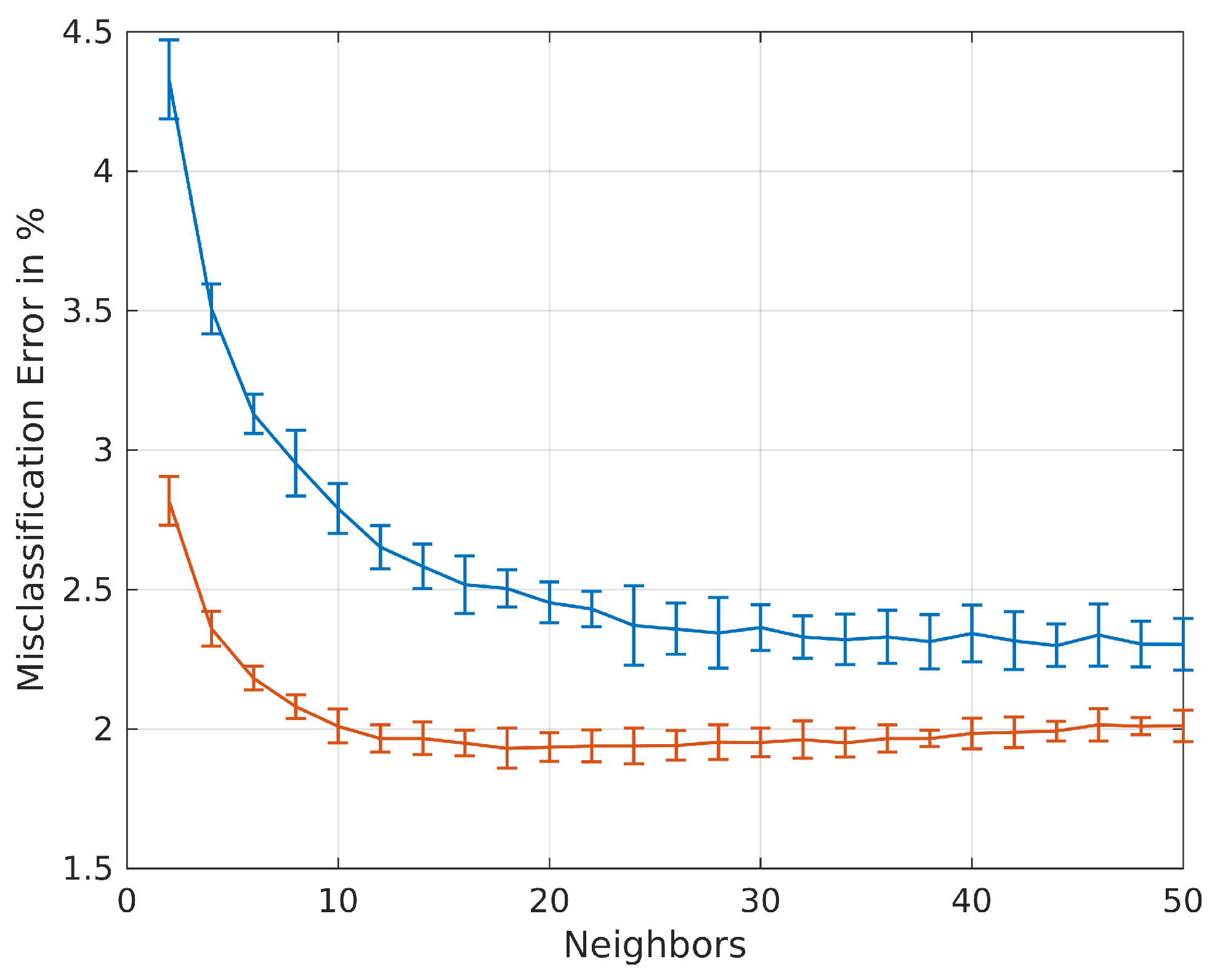
In the present study, K is estimated by performing a 10-fold cross-validation. Therefore the reference model used for the clustering and already assigned to the clusters is divided into 10 randomly sorted, but equally sized subsets and validated against each other. This means, that every subset is used as a test sample and the remaining subsets as training sets. In order to find an appropriate K for K-NN, the cross-validation is performed based on different numbers of neighbors. Figure 6 shows the mean misclassification error as a percentage of the 10-fold cross-validation in the case of SARAL and Envisat. Similar errors can be expected for the classification of the remaining unlabeled waveforms. The minimum error defines the optimal number of neighbors. SARAL displays less variability and a smaller misclassification rate than Envisat. The K-NN method seems to be more stable with clustered SARAL than with Envisat waveforms, which can be explained due to less variability in the AltiKa waveforms and a more robust waveform clustering. For SARAL a minimum error rate is obtained with K = 20 (1.93 ± 0.05%). In the case of Envisat, nearest-neighbor number K = 44 (2.3 ± 0.08%) is used, providing a good balance between low error and variance.
The misclassification rate in connection with the defined number of neighbors gives information about the K-NN prediction error based on the reference model and class labels. This parameter can be used to estimate the internal precision of the classification approach. In this study, a minimal error of about 2% has to be expected from the methodology itself.
After defining an appropriate K, the remaining waveforms are applied to K-NN. In the end of the classification process every waveform is labeled by a certain cluster and, consequently, assigned to a specific surface type.
3.4. Validation Approach
In order to conduct an external validation for the waveform classification, a comparison with independent SAR images is performed. For this purpose, the defined waveform classes of ocean, lead/polynya, sea ice are assigned to water (ones) and non-water (zeros) observations. Undefined waveforms classes are also labeled with zeros. In order to provide quantitative information about the classification performance, it is necessary to compare the results to an external dataset. For this purpose, imaging SAR data are used, as they regularly provide snapshots of different sea surface states in the study area.
Before performing an automatic comparison between SAR and the classification results, the SAR images are pre-processed by using the ESA toolbox SNAP, version 4.0.0 for Sentinel-1A as well as Radarsat-2 and the MapReady toolbox, version 3.1.22 for ALOS image data offered by ASF. Basically, the following standard routines are applied to the imaging SAR data:
- Thermal noise removal (only S-1A)
- Radiometric calibration
- Speckle filter (only Radarsat-2)
- Delay Doppler terrain correction
- Reprojection to Lambert Azimuthal Equal Area map projection
- Converting backscatter values to db
- Datatype conversion in uint8
On the pre-processed SAR images, linear and circular shaped black and near black areas indicate openings inside the sea ice cover generated by a smooth surface and specular reflection of the radar waves. To automatically extract these areas, the SAR images have to be converted into binary pixel values by applying several image processing tools. The applied approach is described in detail by Passaro et al. [14]. Briefly summarized, the images undergo a noise and minimum filtering in order to emphasize dark pixel regions, followed by an adaptive thresholding that considers local illumination changes. Finally, a mathematic morphological closing operation is applied to the black and white coded images to link fragmented open water regions. To control the effect of the morphological closing operation a structure element (kernel) or convolution matrix is needed. Regarding linear and circular shapes of open water areas, an octagon with various size, considering the nominal pixel spacing of the SAR images, is employed. In the case of ALOS, the octagon size is six pixels around the center pixel, and in the case of Sentinel-1A and Radarsat-2, a kernel size of 12 pixels is used. Moreover, the image coordinates are shifted to compensate for sea ice-motion, for the acquisition time difference between altimetry and SAR (see Section 2.4). In a last step, the locations of the altimetry returns are interpolated to the SAR pixel locations by using nearest neighbor method.
4. Results and Discussion
In this study, 15,025 Envisat and 19,919 SARAL observations are investigated for which SAR image classification results are available for validation. 31.2% of the Envisat waveforms and 15.0% of the SARAL returns are assigned to water classes. Furthermore, 4.7% of Envisat and 14.2% of SARAL waveforms are set to undefined and defined as non-water returns. For a quantitative rating, 19 comparison pairs for SARAL and Envisat, respectively (see Section 2.3), are used. The results of this comparison are presented in the following section. Afterwards, examples are displayed to illustrate and discuss the functionality of the validation approach.
4.1. Automatic Comparison to SAR Images
As mentioned above, the automatic comparison process only relies on observations in areas with a semi-closed sea ice layer. This allows one to reduce false SAR classifications outside the ice edge due to an unreliable SAR image processing. Table 4 provides the numbers of measurements assigned to water and ice by the two observation techniques and, therefore, allows for an assessment of the altimetry classification performance. The absolute number of water and ice detections are listed column-wise for the altimetry classification results and row-wise for the SAR open water detection. The table shows that 1124 of the 15025 Envisat observations are identified as water by both, altimetry and SAR, whereas 837 locations are assigned to non-water by altimetry and to water by SAR. Assuming the SAR to be the ground truth validating the altimetry water detection, four dependencies are derived to rate the classification results. The total consistency rate, is computed by summing up the bold values and dividing them by the total number of comparison points. In addition, three conditional frequencies are derived: The true water detection rate () is computed by dividing the “correct” altimetry water detections by the total number of SAR water observations, whereas the false water detection rate () is defined as the relation between the water altimetry detections not confirmed by SAR and the total number of SAR ice detections. Moreover, the percentage of correctly classified water returns represents the “correct” water altimetry detections in relation to the total number of open water detections by altimetry.
In the case of Envisat, a consistency rate of 70.7% is reached. In detail, nearly 60% of SAR water detections are truly classified by Envisat () in contrast to below 30% of SAR ice observations that are falsely assigned to water areas by Envisat (). However, only about a quarter of all Envisat open water detections are also classified by SAR ().
The comparison between SARAL and Sentinel-1A water detection yields a higher consistency rate of 76.9% but a smaller true water detection rate of less than 30% (). At the same time, the false water detection rate is very small and yields only 12.3%. Moreover, the correctly classified water return rate is better as for Envisat.
It has to be noticed that for the interpretation of these numbers it is important to consider that inconsistencies are not only due to altimetry classification but that the SAR open water detection as well as the sea ice-motion correction also contribute to the error budget. For example, most of the SARAL comparisons take place during the sea ice maximum between January and mid March, when the pack ice is very close and exhibits only small openings in the ice, which makes it challenging to be detected by the SAR image processing.
Analyzing the absolute water detection numbers of Envisat versus SAR images, it is remarkable that the number of open water points differs by 2732 between the SAR detection and the Envisat classification. The Envisat classification identifies significantly more open water areas than the SAR processing (factor of nearly 2.4). In the case of SARAL, a transposed situation can be found. This can be explained by different SAR sensor characteristics and an insufficient pixel resolution as well as an imprecise SAR image processing, including an unreliable sea ice-motion correction. Additionally, the altimeters are affected by off-nadir returns, which can cause an enhanced number of open water detections. In the case of Envisat, a larger footprint size than SARAL intensifies off-nadir effects.
Overall, it is important to understand, that the classification performance numbers of SARAL and Envisat are not directly comparable with each other. The underlying different instrumental, sensor, and spatio-temporal conditions differ too strongly to provide qualitative information that would allow for a comparative assessment of the two altimetry satellites. More details related to the impacts of SAR and altimetry processing on the quantitative comparison process can be found in Section 4.2.
Analyzing, for example, of Envisat and SARAL, the quantitative comparison confirms the reliability of the altimetry-based classification method and a good performance of their results. However, it has to be kept in mind that a data comparison of two totally different Earth observation techniques for open water detection in a very dynamic study area is not possible without a variety of uncertainties and inaccuracies. In order to provide a better impression of the difficulties of a quantitative comparison approach, the next section shows a couple of examples in a visual comparison.
4.2. Visual Comparison
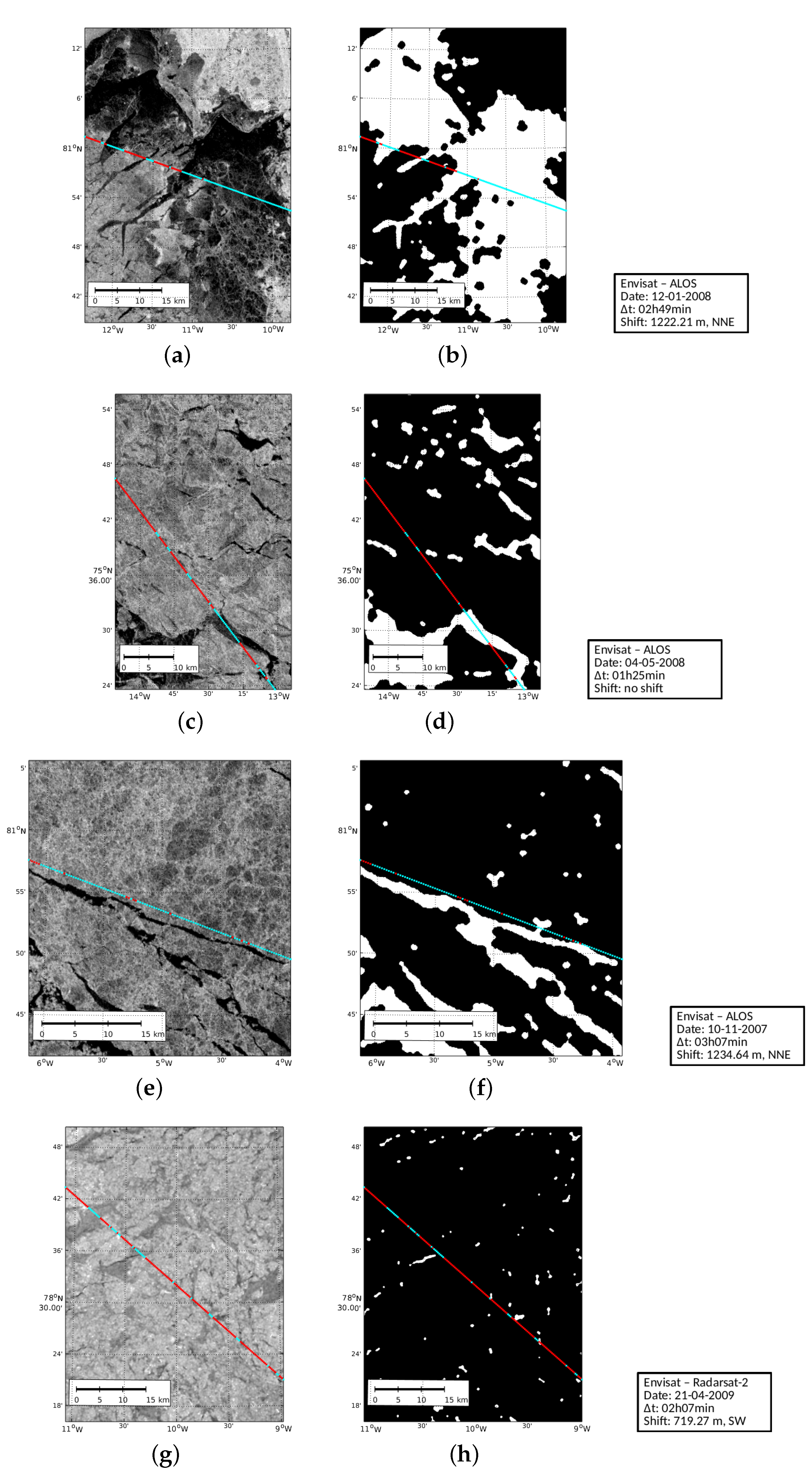
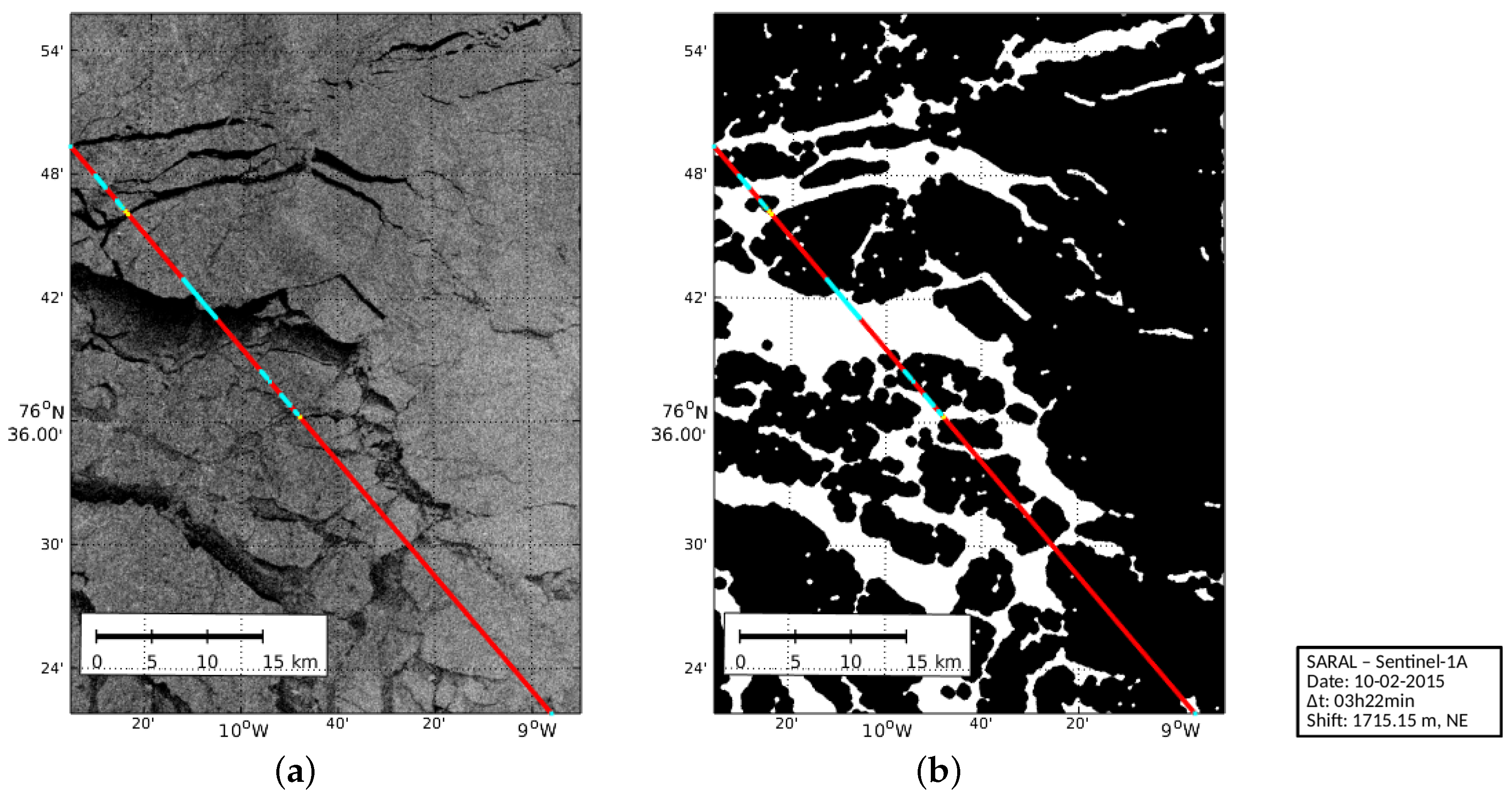
Using different SAR image subsets, this section will provide some visual comparisons between open water classification by altimetry and SAR images. The images were selected in order to indicate possible difficulties due to uncertainties in the SAR image or altimetry processing as well as sea ice motion correction. Figure 7 and Figure 8 show five visual examples before (left) and after (right) image processing. The altimetry measurement locations are superimposed on the SAR image. Cyan colored altimetry observations identify open water classifications. These regions are plotted in white in the binary coded SAR images (right column). Figure 7a–f display Envisat-ALOS and Figure 7g,h Envisat—Radarsat-2 comparisons. Figure 8 shows a visual example of one SARAL—Sentinel-1A comparison. Metadata information, i.e., acquisition date and applied sea ice motion correction on each comparison is provided next to the images (visualized classification results without class assignment can be found in supplementary Fig. S2–S6). Moreover, Table 5 displays quantitative comparison results.
The first example (Figure 7a) demonstrates very good accordance between altimetry and SAR classification.The L-band image displays different sea ice and open water conditions. From West to East, various sized open water areas ranging from 200 m up to 3.5 km are visible. A large region appearing in dark reaches from the image center at W to the eastern edge. It indicates a mixture of differently sized ice floes interrupted by open water sections. Analyzing the colored altimetry observations, the open water detection is in good accordance with the grayscaled as well as with the binary coded SAR image (Figure 7b). The quantitative comparison yields a consistency rate of 90.63%. Moreover, the altimetry classification approach provides a true classification rate close to 100% (). This comprises small leads as well as larger areas of open water.
An almost perfect accordance between altimetry classification and SAR images can also be observed in Figure 7c, detecting an expanded lead in the southern image part and some small leads in the central part of the image. However, comparing Figure 7c and d to the altimetry classification results at N, it is clearly visible that SAR image processing is not always able to segment very narrow lead fragments. This might happen because of a poor spatial pixel resolution of the SAR sensor (100 m), an insufficient identification of the ice-water transition, or a too restrictive threshold level in the SAR image processing. This deficiency in the automatic SAR image processing results in reduced performance in the quantitative comparison with a total consistency rate of about 85% and a true water detection rate of 88.6%.
However, there are also problems related to the altimetry observation technique. The example displayed in Figure 7e,f is characterized by a very long (ca. 47 km) and in most parts narrow lead located parallel to the satellite track. The SAR image is shifted about 1.2 km in the northeastern direction, assuming a steady sea ice motion. Even if the altimeter track is still located northwards at the off-nadir position of the lead, almost all measurements are classified as open water. As a consequence, in the quantitative comparison, just 2% of all Envisat open water detections are confirmed by SAR classification although they can be visually connected with the dominant lead in the image center. The overall consistency rate yields only 12.6%—probably due to the fact that the altimetry classification approach is not able to separate off-nadir water returns from nadir water returns or the mean sea ice motion correction is not enough to consider the total sea ice drift.
Additional discrepancies between altimetry and SAR classification can occur in areas with new, very thin ice coverage. Figure 7g shows those areas, appearing light gray in C-band, only a little darker than the surrounding older ice. These areas are correctly set to ice by the SAR image processing (see Figure 7h) because of the small brightness differences between the thin and surrounding ice types. In contrast, the altimetry returns within these areas are falsely classified and interpreted as calm open water since they show a very narrow and single-peaked lead/polynya-like shape. One explanation for this mis-interpretation is the dominant scattering of all flat and specular surfaces. Connor et al. [11] found that strong reflective surfaces, for example, leads/polynyas, can also affect the waveform shape if covered by very thin ice. A distinction from open water is not possible based on the altimetry waveform’s shape. Since the ice is very thin, the retracked ranges should represent the water level well enough, even if the classification is wrong.
Related to the comparison process itself, uncertainties in sea ice motion correction can reduce the quantitative consistency rate. Figure 8a,b are corrected by ice-motion considering a time difference of more than 3 h. Analyzing Figure 8b, it can be shown that only 25.53% of the SAR detected ice openings are well identified by the altimetry data. A visual image inspection suggests that the applied ice motion correction is too small to completely compensate for the effect of the time lag.
Further challenging issues using SARAL SGDR-T data are so-called saturated waveforms. Zakharova et al. [12] pointed out that leads or strongly reflecting surfaces can exceed the maximum permissible power count value of 1250. The waveforms are cut and feature no clear peak due to a saturated power tracking window. Figure 8 highlights saturated SARAL observations in yellow. They are mainly located near small and calm open water areas, producing very high backscatter returns. In the classification process, they are omitted because of an unknown maximum peak position. In general, saturated SARAL waveforms are mainly traceable within the sea ice edge, but can provide evidence about the location of further open water areas. However, just 0.14% (i.e., 288 waveforms) of the comparison data are affected by a saturated power tracking window.
The present section shows a number of challenging and unavoidable impacts on the validation of the waveform classification process. Considerable parts of the inconsistencies do not originate from the altimetry classification but from the SAR classification or the ice-motion correction. In order to adequately rate the quantitative comparison results, it is necessary to keep these effects in mind.
5. Conclusions and Outlook
The present paper introduces an unsupervised classification approach based on pulse-limited multi-mission altimetry data to detect open water areas in a largely sea ice covered region. The study demonstrates the successful application of the clustering of pulse-limited altimeter waveforms for the automatic identification of open ocean, sea ice, lead and polynya observations. The approach is based on known partition cluster strategies (i.e., K-medoids) and memory-based classification methods (i.e., K-nearest-neighbor). A 10-fold cross-validation for the assessment of the precision of the classification method is performed. It indicates an internal misclassification error of about 2% for Envisat and SARAL. The algorithm is applicable to every pulse-limited altimetry satellite mission without requiring any deeper knowledge about mission specific details. Moreover, it can be assumed that the developed approach also works for SAR altimetry waveforms if the waveform feature space is adapted adequately. Additionally, the presented method can be adapted to a number of open water detection or waveform classification tasks, e.g., for the identification of lake returns [33] or in inundation areas.
In order to evaluate the classification results, a comparison with SAR images is performed. In contrast to previous studies, the present validation relies not only on visual and manually selected examples, but also on a larger set of images and an automated comparison procedure. The comparison procedure allows for a quantitative assessment of the classification performance by assigning the altimetry observations to open water and sea ice returns and checking them against processed SAR images that indicate sea ice and open water areas. We reach consistency rates of 70.7% for Envisat and 76.9% for SARAL. However, it has to be underlined that the quantitative comparison results of Envisat and SARAL are not directly comparable because of significant differences in the underlying sensor and instrument characteristics of the available SAR missions.
When interpreting the comparison results, different sources of inconsistencies have to be considered, e.g., effects from the altimetry data and their classification procedure and uncertainties in SAR image processing as well as in the ice-motion correction. The Fram Strait and the Greenland Sea are one of the most dynamic areas on Earth. Fast changing sea ice conditions due to short, periodic melting and refreezing as well as rapid climate change make it hard to provide a high reliability in the comparison as well as in the altimetry classification results. Local phenomena, such as melt ponds (i.e., open water pools on the sea ice surface) and their impacts on the open-water detection, have to be investigated. Over specific sea ice types, altimetry waveforms show ambiguities, which prevents a clear attribution to sea ice or open water returns. In particular, specular thin and flat ice produces very specular returns resembling open water returns. In contrast, big ice floes or landfast ice can imitate ocean-like returns due to similarities in ocean surface roughness and reflectivity.
Further improvements of the classification method are possible. In particular, saturated SARAL waveforms have to be included in the classification process. In addition, the application of more recent sea ice motion data in combination with Sentinel-1B data could lead to a better spatio-temporal ratio within the validation process.
A reliable classification is an indispensable requirement for a meaningful estimation and an efficient computation of sea surface heights in the Arctic by retracking only open water waveforms. In addition to Envisat and SARAL, more pulse-limited (e.g., ERS-1/2) as well as delay-doppler altimetry data (e.g., CryoSat-2, Sentinel-3A) may be employed in the classification process and, thus, contribute to the generation of a long-term sea level record for the Arctic ocean.
Supplementary Materials
The following folder and figures are available online at www.mdpi.com/2072-4292/9/6/551/s1, Figure S1 displays SARAL waveform clusters, Figures S2–S6 and folder S2 contain Figure 7 and Figure 8 showing the classification results without class assignment.
Acknowledgments
The authors thank the following institutions and agencies for providing their data and software products under the terms of the GNU General Public License. ESA for operating and managing Envisat, Sentinel-1A and the SNAP Toolbox. CNES for providing SARAL data. JAXA/METI and ASF DAAC for making ALOS PALSAR L1.5 data and MapReady Toolbox available as well ESA for maintaining MDA Radarsat-2 data in framework of Third Party Mission program. This work was supported by the German Research Foundation (DFG) through grants, BO1228/13-1 and DE2174/3-1. The publication is funded by the Technical University of Munich (TUM) within the framework of the Open Access Publishing Program. We thank five anonymous reviewers for their valuable comments that helped to improve the manuscript.
Author Contributions
Felix L. Müller developed the classification and validation methods, conducted the data analysis and wrote the majority of the paper. Denise Dettmering supervised the present study, contributed to the manuscript writing and helped with the discussions of the applied methods and results. Wolfgang Bosch initiated the study. Florian Seitz supervised the research. Both were involved in the writing process and discussed the methods presented in the manuscript as well.
Conflicts of Interest
The authors declare no conflict of interest.
References
- Comiso, J. Polar Oceans from Space; Atmospheric and Oceanographic Sciences Library, Springer: New York, NY, USA, 2010. [Google Scholar]
- Stroeve, J.C.; Markus, T.; Boisvert, L.; Miller, J.; Barrett, A. Changes in Arctic melt season and implications for sea ice loss. Geophys. Res. Lett. 2014, 41, 1216–1225. [Google Scholar] [CrossRef]
- Polyakov, I.V.; Beszczynska, A.; Carmack, E.C.; Dmitrenko, I.A.; Fahrbach, E.; Frolov, I.E.; Gerdes, R.; Hansen, E.; Holfort, J.; Ivanov, V.V.; et al. One more step toward a warmer Arctic. Geophys. Res. Lett. 2005, 32, L17605. [Google Scholar] [CrossRef]
- Sasgen, I.; van den Broeke, M.; Bamber, J.L.; Rignot, E.; Sørensen, L.S.; Wouters, B.; Martinec, Z.; Velicogna, I.; Simonsen, S.B. Timing and origin of recent regional ice-mass loss in Greenland. Earth Planet. Sci. Lett. 2012, 333–334, 293–303. [Google Scholar] [CrossRef]
- Laxon, S.W. Sea-Ice Altimeter Processing Scheme at the EODC. Int. J. Remote Sens. 1994, 15, 915–924. [Google Scholar] [CrossRef]
- Rio, M.H.; Hernandez, F. A mean dynamic topography computed over the world ocean from altimetry, in situ measurements, and a geoid model. J. Geophys. Res. Oceans 2004, 109. [Google Scholar] [CrossRef]
- Dwyer, R.; Godin, R. Determining Sea-Ice Boundaries and Ice Roughness Using GEOS-3 Altimeter Data; Technical Report; NASA Wallops Flight Center: Wallops Island, VA, USA, 1980.
- Fetterer, F.M.; Drinkwater, M.R.; Jezek, K.C.; Laxon, S.W.C.; Onstott, R.G.; Ulander, L.M.H. Sea Ice Altimetry. In Microwave Remote Sensing of Sea Ice; American Geophysical Union: Washington, DC, USA, 2013; pp. 111–135. [Google Scholar]
- Laxon, S.; Peacock, N.; Smith, D. High interannual variability of sea ice thickness in the Arctic region. Nature 2003, 425, 947–950. [Google Scholar] [CrossRef] [PubMed]
- Peacock, N.R. Sea surface height determination in the Arctic Ocean from ERS altimetry. J. Geophys. Res. 2004, 109, C07001. [Google Scholar] [CrossRef]
- Connor, L.N.; Laxon, S.W.; Ridout, A.L.; Krabill, W.B.; McAdoo, D.C. Comparison of Envisat radar and airborne laser altimeter measurements over Arctic sea ice. Remote Sens. Environ. 2009, 113, 563–570. [Google Scholar] [CrossRef]
- Zakharova, E.A.; Fleury, S.; Guerreiro, K.; Willmes, S.; Rémy, F.; Kouraev, A.V.; Heinemann, G. Sea Ice Leads Detection Using SARAL/AltiKa Altimeter. Mar. Geod. 2015, 38, 522–533. [Google Scholar] [CrossRef]
- Zygmuntowska, M.; Khvorostovsky, K.; Helm, V.; Sandven, S. Waveform classification of airborne synthetic aperture radar altimeter over Arctic sea ice. Cryosphere 2013, 7, 1315–1324. [Google Scholar] [CrossRef]
- Passaro, M.; Müller, F.L.; Dettmering, D. Lead Detection using Cryosat-2 Delay-Doppler Processing and Sentinel-1 SAR images. Adv. Space Res. 2017. under review. [Google Scholar]
- Rudels, B.; Friedrich, H.J.; Quadfasel, D. The Arctic Circumpolar Boundary Current. Deep-Sea Res. Part II 1999, 46, 1023–1062. [Google Scholar] [CrossRef]
- Serreze, M.; Barry, R. The Arctic Climate System; Cambridge Atmospheric and Space Science Series; Cambridge University Press: Cambridge, UK, 2014. [Google Scholar]
- Bersch, M. On the circulation of the northeastern North Atlantic. Deep-Sea Res. Part II 1995, 42, 1583–1607. [Google Scholar] [CrossRef]
- Woodgate, R.A.; Fahrbach, E.; Rohardt, G. Structure and transports of the East Greenland Current at 75∘N from moored current meters. J. Geophys. Res. Oceans 1999, 104, 18059–18072. [Google Scholar] [CrossRef]
- Verron, J.; Sengenes, P.; Lambin, J.; Noubel, J.; Steunou, N.; Guillot, A.; Picot, N.; Coutin-Faye, S.; Sharma, R.; Gairola, R.M.; et al. The SARAL/AltiKa Altimetry Satellite Mission. Mar. Geod. 2015, 38, 2–21. [Google Scholar] [CrossRef]
- Japan Aerospace Exploration Agency (JAXA). ALOS Data Users Handbook, Revision C; Japan Aerospace Exploration Agency: Chofu, Tokyo, Japan, 2008. [Google Scholar]
- MDA. RADARSAT-2 Product Description; Report RN-SP-52-1238, Issue 1/13; MacDonald, Dettwiler and Associates Ltd.: Vancouver, BC, Canada, 2016. [Google Scholar]
- Sentinel-1 Team. Sentinel-1 User Handbook; GMES-S1OP-EOPG-TN-13-0001, Issue Draft; European Space Agency: Paris, France, 2013. [Google Scholar]
- Dierking, W. Sea Ice Monitoring by Synthetic Aperture Radar. Oceanography 2013, 26. [Google Scholar] [CrossRef]
- Jackson, C.R.; Apel, J.R. Synthetic Aperture Radar: Marine User’s Manual; US Department of Commerce, National Oceanic and Atmospheric Administration, National Environmental Satellite, Data, and Information Serve, Office of Research and Applications: Washington, DC, USA, 2004; pp. 81–115.
- Tschudi, M.; Fowler, C.; Maslanik, J.; Stewart, J.S. Polar Pathfinder Daily 25 km EASE-Grid Sea Ice Motion Vectors, Version 3; Subset: Greenland Sea, Date Accessed: 16.11.2016; National Snow and Ice Data Center: Boulder, CO, USA, 2016. [Google Scholar]
- Cavalieri, D.; Parkinson, C.; Gloersen, P.; Zwally, J.H. Sea Ice Concentrations from Nimbus-7 SMMR and DMSP SSM/I-SSMIS Passive Microwave Data, Version 1; Subset: Greenland Sea, Date Accessed: 16.11.2016; NASA National Snow and Ice Data Center Distributed Active Archive Center: Boulder, CO, USA, 1996.
- Xu, R.; Wunsch, D.C. Clustering; IEEE Press Series on Computational Intelligence; IEEE Press: Hoboken, NJ, USA; Wiley: Piscataway, NJ, USA, 2009. [Google Scholar]
- Hastie, T.; Tibshirani, R.; Friedman, J. The Elements of Statistical Learning; Springer: New York, NY, USA, 2009; Volume 2, pp. 337–387. [Google Scholar]
- Kohonen, T. Self-Organizing Maps; Springer Series in Information Sciences; Springer: Berlin/Heidelberg, Germany, 2012. [Google Scholar]
- Celebi, M. Partitional Clustering Algorithms; EBL-Schweitzer, Springer International Publishing: Cham, Switzerland, 2014. [Google Scholar]
- Kaufman, L.; Rousseeuw, P.J. Finding Groups in Data: An Introduction to Cluster Analysis; Wiley Series in Probability and Mathematical Statistics; Wiley: New York, NY, USA, 1990. [Google Scholar]
- Kvingedal, B. Sea-Ice Extent and Variability in the Nordic Seas, 1967–2002. In The Nordic Seas: An Integrated Perspective; American Geophysical Union: Washington, DC, USA, 2013; pp. 39–49. [Google Scholar]
- Göttl, F.; Dettmering, D.; Müller, F.L.; Schwatke, C. Lake Level Estimation Based on CryoSat-2 SAR Altimetry and Multi-Looked Waveform Classification. Remote Sens. 2016, 8, 885. [Google Scholar] [CrossRef]
Figure 1.
Black rectangles indicate locations of the SAR images from ALOS and Radarsat-2 used for comparison with Envisat classification results against the background of nominal sun-synchronous ground tracks of one Envisat cycle. The four subsets discussed in Section 4.2 are highlighted by different colors.

Figure 2.
Black rectangles indicate locations of the SAR images from Sentinel-1A used for comparison with SARAL classification results against the background of nominal sun-synchronous ground tracks of one SARAL cycle. One subset discussed in Section 4.2 is highlighted in orange.
Figure 2.
Black rectangles indicate locations of the SAR images from Sentinel-1A used for comparison with SARAL classification results against the background of nominal sun-synchronous ground tracks of one SARAL cycle. One subset discussed in Section 4.2 is highlighted in orange.

Figure 3.
Waveform examples for Envisat (top row) and SARAL (bottom row) for three different surface scatterers: Ocean (left), Lead (middle), and Sea Ice (right).
Figure 3.
Waveform examples for Envisat (top row) and SARAL (bottom row) for three different surface scatterers: Ocean (left), Lead (middle), and Sea Ice (right).
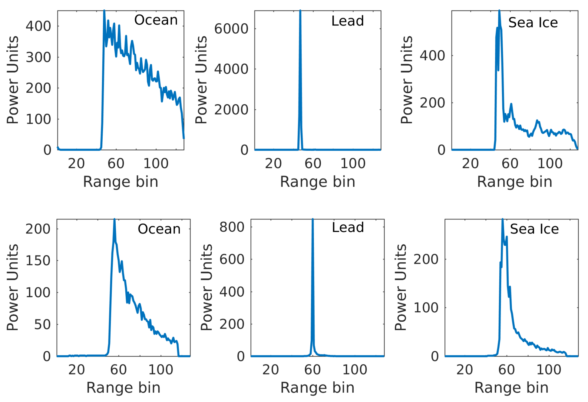
Figure 4.
Envisat waveform clusters (K = 30) after K-medoids clustering showing segmented waveforms (every twenty fifth per cluster).
Figure 4.
Envisat waveform clusters (K = 30) after K-medoids clustering showing segmented waveforms (every twenty fifth per cluster).

Figure 5.
Means and standard deviations of waveform features (see Section 3.1) per cluster. Four classes are illustrated using different colors: “lead/polynya” (cyan), “ocean” (purple), “ice” (green), and “undefined” (red).
Figure 5.
Means and standard deviations of waveform features (see Section 3.1) per cluster. Four classes are illustrated using different colors: “lead/polynya” (cyan), “ocean” (purple), “ice” (green), and “undefined” (red).
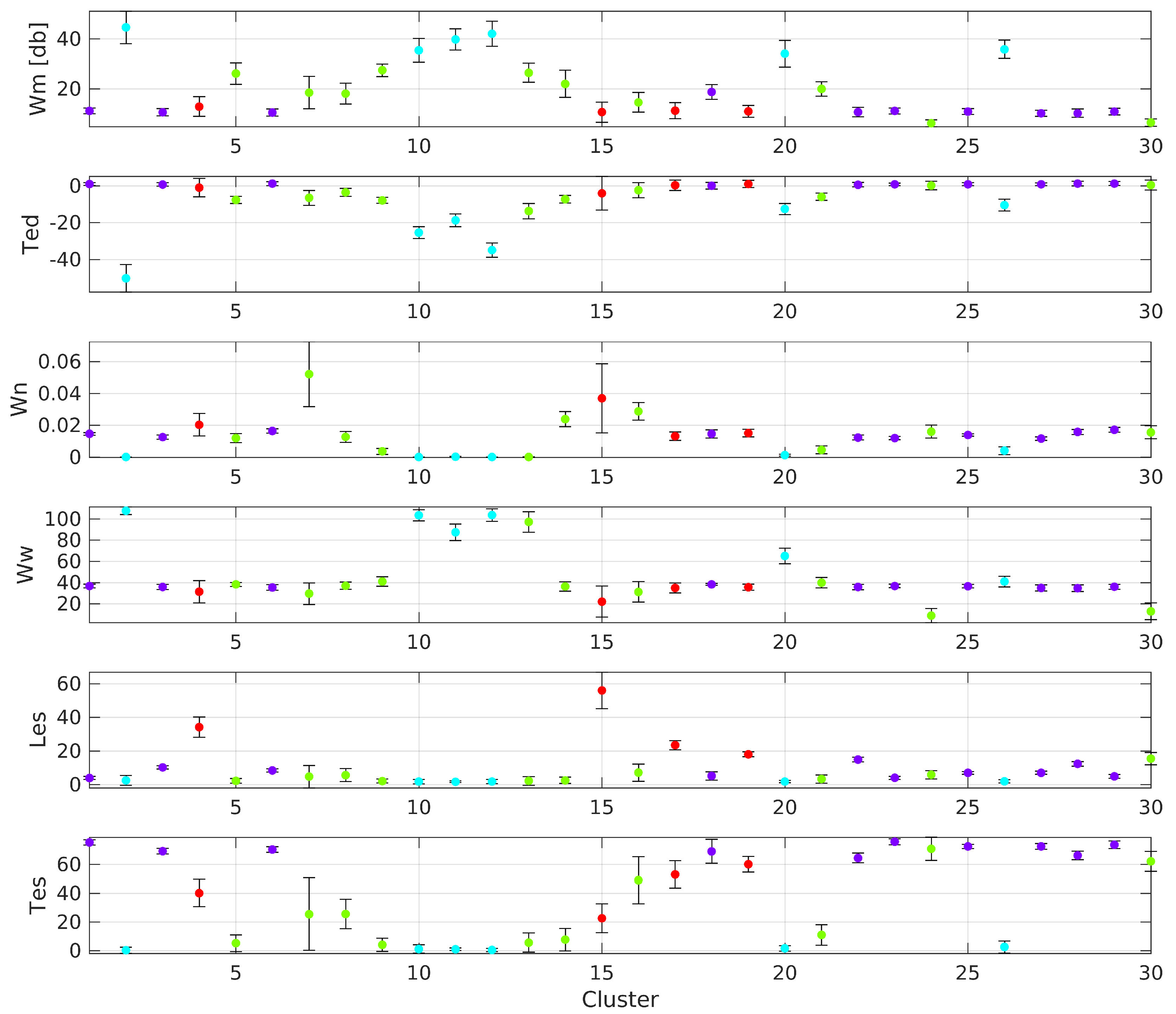
Figure 6.
Misclassification error and its standard deviation for SARAL (red) and Envisat (blue) with varying number of K neighbors as computed by 10-fold cross-validation.
Figure 6.
Misclassification error and its standard deviation for SARAL (red) and Envisat (blue) with varying number of K neighbors as computed by 10-fold cross-validation.

Figure 7.
Examples of open water detection from Envisat against ALOS (a–f) and Radarsat-2 (g,h) before (left) and after SAR image processing (right) with open water indicated in white. Boxes provide additional image and processing information. Red: ice detection, cyan: open water detection. The geographical locations of the image subsets are displayed in Figure 1; from top to bottom in green, blue, yellow and magenta.

Figure 8.
Example (orange highlighted in Figure 2) of open water detection from SARAL against Sentinel-1A before (a) and after SAR image processing (b) with open water indicated in white. Box provides additional image and processing information. Red: ice detection, cyan: open water detection, yellow: saturated AltiKa observations.


Table 1.
Synthetic Aperture Radar (SAR) image specifications [20,21,22] and altimeter satellites covering same time periods.
| SAR Satellite | Band | Mode | Swath Width (km) | Pixel Size (m) | Period (mm/yyyy) | Altimeter Satellite |
|---|---|---|---|---|---|---|
| ALOS | L-Band | Wide Beam | 250–350 | 100 × 100 | June 2007–May 2008 | Envisat |
| Radarsat-2 | C-Band | Scan SAR Wide | 500 | 50 × 50 | June 2008–present | Envisat/SARAL |
| Sentinel-1A | C-Band | Extra Wide | 400 | 40 × 40 | October 2014–present | SARAL |
Table 2.
Acquisition date of the SAR images and time gap between altimetry observations and imaging data used for comparison with Envisat classification results.
Table 2.
Acquisition date of the SAR images and time gap between altimetry observations and imaging data used for comparison with Envisat classification results.
| SAR-Satellite | Acquisition Date | Time Gap hh-mm |
|---|---|---|
| ALOS | 14 June 2007 | 02-30 |
| ALOS | 1 October 2007 | 02-57 |
| ALOS | 7 October 2007 | 01-55 |
| ALOS | 10 November 2007 | 03-07 |
| ALOS | 10 December 2007 | 02-50 |
| ALOS | 26 December 2007 | 02-13 |
| ALOS | 5 January 2008 | 02-40 |
| ALOS | 7 January 2008 | 01-46 |
| ALOS | 12 January 2008 | 02-49 |
| ALOS | 4 May 2008 | 01-25 |
| R-2 | 4 November 2008 | 01-47 |
| R-2 | 20 April 2009 | 02-09 |
| 00-29 | ||
| R-2 | 21 April 2009 | 02-07 |
| R-2 | 10 February 2010 | 03-04 |
| 01-52 | ||
| R-2 | 14 March 2010 | 00-13 |
| 01-27 | ||
| R-2 | 16 October 2010 | 02-04 |
Table 3.
Sentinel-1A acquisition date of the SAR images and time gap between altimetry observations and imaging data used for comparison with SARAL classification results.
Table 3.
Sentinel-1A acquisition date of the SAR images and time gap between altimetry observations and imaging data used for comparison with SARAL classification results.
| Acquisition Date | Time Gap hh-mm |
|---|---|
| 23 October 2014 | 02-41 |
| 16 November 2014 | 03-34 |
| 14 November 2014 | 02-49 |
| 18 November 2014 | 02-42 |
| 3 December 2014 | 02-40 |
| 6 December 2014 | 02-58 |
| 27 December 2014 | 03-33 |
| 1 January 2015 | 02-59 |
| 15 January 2015 | 03-20 |
| 18 January 2015 | 03-27 |
| 16 March 2015 | 03-08 |
| 6 February 2015 | 03-29 |
| 6 February 2015 | 03-28 |
| 10 February 2015 | 03-22 |
| 22 February 2015 | 02-59 |
| 2 March 2015 | 02-44 |
| 9 March 2015 | 02-56 |
| 19 April 2015 | 02-53 |
| 15 May 2015 | 02-54 |
Table 4.
2D contingency tables based on Envisat—ALOS/R-2 (top) and SARAL—S-1A (bottom) comparisons. The table shows the number of points classified as water/ice from altimetry (Alt) with the corresponding classification from SAR.
Table 4.
2D contingency tables based on Envisat—ALOS/R-2 (top) and SARAL—S-1A (bottom) comparisons. The table shows the number of points classified as water/ice from altimetry (Alt) with the corresponding classification from SAR.
| Alt (Water) | Alt (Ice) | ∑ | |
|---|---|---|---|
| SAR (water) | 1124 | 837 | 1961 |
| SAR (ice) | 3569 | 9495 | 13064 |
| ∑ | 4693 | 10332 | 15025 |
| Alt (Water) | Alt (Ice) | ∑ | |
| SAR (water) | 987 | 2600 | 3587 |
| SAR (ice) | 2007 | 14325 | 16332 |
| ∑ | 2994 | 16925 | 19919 |
Table 5.
Table providing percentage statistical information about conditional and consistency rates of visual examples discussed in Section 4.2. “SAR” and “Alt” indicate imaging SAR and altimetry. Ice detections are indexed by overline character marked shortcuts.
Table 5.
Table providing percentage statistical information about conditional and consistency rates of visual examples discussed in Section 4.2. “SAR” and “Alt” indicate imaging SAR and altimetry. Ice detections are indexed by overline character marked shortcuts.
| Subset | ||||
|---|---|---|---|---|
| Figure 7b | 90.63% | 15.91% | 91.86% | 94.05% |
| Figure 7d | 85.10% | 16.04% | 64.58% | 88.57% |
| Figure 7f | 12.61% | 88.99% | 2.02% | 100.00% |
| Figure 7h | 76.22% | 22.36% | 0.00% | 0.00% |
| Figure 8b | 72.07% | 12.41% | 40.68% | 25.53% |
© 2017 by the authors. Licensee MDPI, Basel, Switzerland. This article is an open access article distributed under the terms and conditions of the Creative Commons Attribution (CC BY) license (http://creativecommons.org/licenses/by/4.0/).
Share and Cite
MDPI and ACS Style
Müller, F.L.; Dettmering, D.; Bosch, W.; Seitz, F. Monitoring the Arctic Seas: How Satellite Altimetry Can Be Used to Detect Open Water in Sea-Ice Regions. Remote Sens. 2017, 9, 551. https://doi.org/10.3390/rs9060551
AMA Style
Müller FL, Dettmering D, Bosch W, Seitz F. Monitoring the Arctic Seas: How Satellite Altimetry Can Be Used to Detect Open Water in Sea-Ice Regions. Remote Sensing. 2017; 9(6):551. https://doi.org/10.3390/rs9060551
Chicago/Turabian StyleMüller, Felix L., Denise Dettmering, Wolfgang Bosch, and Florian Seitz. 2017. "Monitoring the Arctic Seas: How Satellite Altimetry Can Be Used to Detect Open Water in Sea-Ice Regions" Remote Sensing 9, no. 6: 551. https://doi.org/10.3390/rs9060551
Note that from the first issue of 2016, this journal uses article numbers instead of page numbers. See further details here.