Article

Moving to the RADARSAT Constellation Mission: Comparing Synthesized Compact Polarimetry and Dual Polarimetry Data with Fully Polarimetric RADARSAT-2 Data for Image Classification of Peatlands

1
Environment and Climate Change Canada, National Wildlife Research Centre, 1125 Colonel by Drive, Ottawa, ON K1S 5B6, Canada
2
Department of Geography and Environmental Studies, Carleton University, 1125 colonel By Drive, Ottawa, ON K1S 5B6, Canada
3
Defence Research and Development Canada (DRDC), Ottawa Research Center, 3701 Carling Ave., Ottawa, ON K2K 2Y7, Canada
*
Author to whom correspondence should be addressed.
Remote Sens. 2017, 9(6), 573; https://doi.org/10.3390/rs9060573
Submission received: 7 April 2017 / Revised: 19 May 2017 / Accepted: 4 June 2017 / Published: 7 June 2017

Abstract

:
For this research, the Random Forest (RF) classifier was used to evaluate the potential of simulated RADARSAT Constellation Mission (RCM) data for mapping landcover within peatlands. Alfred Bog, a large peatland complex in Southern Ontario, was used as a test case. The goal of this research was to prepare for the launch of the upcoming RCM by evaluating three simulated RCM polarizations for mapping landcover within peatlands. We examined (1) if a lower RCM noise equivalent sigma zero (NESZ) affects classification accuracy, (2) which variables are most important for classification, and (3) whether classification accuracy is affected by the use of simulated RCM data in place of the fully polarimetric RADARSAT-2. Results showed that the two RCM NESZs (−25 dB and −19 dB) and three polarizations (compact polarimetry, HH+HV, and VV+VH) that were evaluated were all able to achieve acceptable classification accuracies when combined with optical data and a digital elevation model (DEM). Optical variables were consistently ranked to be the most important for mapping landcover within peatlands, but the inclusion of SAR variables did increase overall accuracy, indicating that a multi-sensor approach is preferred. There was no significant difference between the RF classifications which included RADARSAT-2 and simulated RCM data. Both medium- and high-resolution compact polarimetry and dual polarimetric RCM data appear to be suitable for mapping landcover within peatlands when combined with optical data and a DEM.

Graphical Abstract

1. Introduction

Peatlands are a unique class of wetlands with many important functions including storing carbon, providing habitat for several wildlife species, mitigating floods and droughts, as well as retaining, purifying, and releasing water [1]. Peatlands account for roughly 12% of Canada’s land cover [2], and approximately 40% of the world’s peatlands are found within Canada [3]. Peatlands can be defined as land that has a surface layer of naturally accumulated peat [4], and peat is described as soil that contains a minimum of 30% (by dry mass) dead organic material [5]. Bogs and fens are two sub-classes of peatlands. Rainwater is the main source of water and mineral nutrients for bogs, while fens obtain their mineral rich water from soil [3].
Peatlands that have remained in their natural state for years are able to store carbon because typically the rate of plant production and peat accumulation is greater than the rate of organic matter decomposition [6]. However, the agriculture and forestry industries often drain peatlands, transforming them from carbon sinks into net sources of Greenhouse Gases (GHGs) [6]. In recent years, there has been concern over how peatlands are being managed and how they will react to climate change in the future. It is expected that the increases in temperature and evapotranspiration anticipated with climate change will result in surface drying and a decreased water table in many wetlands [7]. In order to sustainably manage and conserve peatlands an up-to-date peatland inventory is needed to track peatland loss and estimate emissions of GHGs.
Remote sensing technology offers a practical approach to map and monitor peatlands systematically, and at large spatial scales. Many of Canada’s peatlands are in remote locations, making the collection of ground data challenging and costly [8,9]. Optical satellites have been used to map wetlands, including peatlands, for many years [10,11,12,13,14]. Several optical satellites have data in the visible, near infrared and shortwave infrared portions of the electromagnetic spectrum. The near-infrared bands have been shown to improve class separability of wetland types because they can better detect different hydrological conditions and plant species [8]. Nevertheless, optical satellites are passive sensors that require the sun to detect reflected and emitted energy. Thus, they can only acquire images in daylight and can be hindered by cloud cover and haze. Additionally, optical sensors cannot penetrate vegetation canopies, which often preclude the discrimination of classes on the basis of sub-canopy or ground surface conditions like the volumetric moisture of soil, which tends to vary among different wetland types. This makes mapping densely vegetated areas difficult [15].
Due to the limitations with optical satellites and the complexity of mapping wetlands, many remote sensing scientists have begun fusing optical and SAR data to classify wetlands (e.g., [16,17,18,19,20,21,22]). SAR systems operate at longer wavelengths, allowing incident microwaves to penetrate the vegetation canopy to some degree. Thus, SAR backscatter can provide information on sub-surface conditions like soil moisture, though it is also affected by other properties of ground targets, including surface roughness, surface water, and vegetative biomass [20]. In addition to wavelength, SAR backscatter is also affected by incidence angle and polarization [20]. Consequently, a variety of wavelengths, polarizations, and incidence angles will provide more information about the surface, potentially improving the ability to detect different wetland types.
Currently, many SAR satellites are multi-polarized, which has improved the detection of soil moisture and inundation compared to single polarized systems [23,24]. In a single polarized SAR system, both the transmitted and received energy sent by the satellite fall along the same plane: horizontally (H) or vertically (V), relative to the SAR look direction. Dual polarized SAR systems can send and receive energy as either co-polarized (both the transmitted and received energy are HH or VV, where the first letter denotes the transmitted polarization and the last letter denotes the received polarization) or cross-polarized (transmitted and received as HV or VH).
Quad-polarized (i.e., fully polarimetric) SAR sensors are able to transmit and receive the signal in four planes (HH, VV, HV, and VH) [25], and measure the relative phase between channels. The latter represents the time it takes for the radar signal sent from the satellite to reach the ground target and return [26]. The additional information provided by the phase allows for the SAR backscatter to be decomposed into different scattering types important for wetland mapping, including: specular scattering, which is when no energy is returned to the satellite and results from smooth surfaces (e.g., smooth, open water); rough surface scattering, when objects return a single bounce to the satellite (e.g., small shrubs or rough water); volume scattering, defined as backscatter return in multiple directions, which can be caused by features like vegetation canopies; and double-bounce, which arises when two smooth surfaces make a right angle that redirects the incoming radar signal off both surfaces, resulting in most of the signal being returned to the satellite (e.g., emergent vegetation surrounded by smooth open water) [25,26,27,28,29,30].

2. Background

Quad-polarized RADARSAT-2 data has proven useful for wetland mapping [25,31,32,33]. Nonetheless, this polarization is only available in a narrow swath size, limiting the ability to map wetlands operationally, and for large areas. Canada is planning to launch the next generation of C-band SAR satellites, called the RADARSAT Constellation Mission (RCM), which will have multiple different polarizations available (Table 1). It is anticipated to be launched in 2018 and will mainly focus on operational monitoring. RCM will be comprised of three identical C-band SAR satellites launched simultaneously allowing for daily coverage over Canada with 350 km imaging swaths [34]. This will allow for a much shorter repeat cycle, offering a coherent change detection (CCD) timeframe of 4 days (resulting from the three satellites) [34], temporal datasets, and more flexibility and reliability compared to RADARSAT-1 and RADARSAT-2 [35]. One of the primary polarization options will be compact polarimetry (CP), which will be available for all RCM imaging modes. The focus of this study was to investigate the potential of a single RCM scene for peatland classification since acquiring processing and analysing multi-temporal data is computationally expensive and, as shown in this case, may not be necessary if one has optical data. Future research will focus on evaluating CCD with RCM for mapping seasonal changes in wetlands, as RADARSAT-2 has shown promising results [36].
Circular-linear CP SAR systems send out a circularly polarized wave and receive the signal on the linear, horizontal, and linear vertical planes, while maintaining the phase [37]. The rationale for offering a CP mode is that users can be provided with nearly the same information content as quad-polarization data, but at a much larger swath width [34]. In order to be able to provide an increase in swath width, however, there will be a higher noise equivalent sigma zero (NESZ, loss in radiometry, resulting in less sensitivity to low values of backscatter) for all RCM polarizations. In addition, CP will have less polarization diversity compared to the quad polarimetric data available on RADARSAT-2, because it will only capture two channels of data: RH (right circular—linear horizontal polarization) and RV (right circular—linear vertical polarization). In contrast, RADARSAT-2 captures data measured coherently in four channels: HH, HV, VH, and VV [38].
To prepare for the upcoming RCM, the Canadian Space Agency (CSA) has provided funding to Canadian Government Departments to evaluate a variety of RCM polarization options and provide recommendations regarding the effect of polarization, resolution and noise floor for monitoring a variety landscapes operationally. Environment and Climate Change Canada (ECCC) is responsible for providing CSA with RCM recommendations focused around wetland mapping. These preferences will be considered by the CSA when determining the background mission.

2.1. Random Forest

Random Forest (RF) is a machine learning classifier that is commonly used to fuse multiple sources of remote sensing data for wetland mapping [39,40,41]. RF grows several individual decision tree classifiers using random bootstrap aggregated sampling (bagging) [42]. For supervised classifications, a bootstrap sample (two thirds) from user provided training data is used to build each decision tree, and the remaining training samples (one third) are used for internal validation, referred to as the out of bag error (OOBE). The training data are returned to the data pool after each bootstrapping iteration, which allows for different training subsets for all trees. The algorithm selects the best fitting predictor variable from a random group of predictor variables to determine the split at each node and create smaller binary classes [43,44]. A voting mechanism is used to determine the final class prediction. This is achieved by running values down all built trees. Each tree then provides a single vote, and the majority vote is calculated. This approach attempts to eliminate errors within individual trees because it assumes that these errors have not been included in the majority of trees [45,46,47,48].
RF generates two measures of variable importance, the Gini Index and the Mean Decrease in Accuracy. The Gini Index provides an estimate of how pure the node is for each variable, and the Mean Decrease in accuracy calculates the relative change in accuracy when the variable is removed from the model. A higher value in either suggests that the variable is more important [39,42,44]. These measures allow the user to determine which variables have the best predictive power in the final classification. Additionally, variables can be removed from the models that have low importance rankings, which can decrease processing times and improve model accuracy [40,49,50].
The RF algorithm has a number of advantages over some traditional classification methods. For example, RF can be used with data that is not normally distributed [42]. In contrast, this is an underlying assumption of the Maximum Likelihood approach [51]. By determining the split at each node, correlation between individual trees is reduced, and allows for the use of both independent and dependent data [42,45,52,53,54]. Additionally, because only a portion of the variables are used when deciding the split at each node, RF is more computationally efficient than other methods, increasing the ability to incorporate highly dimensional datasets [45,52,53].

2.2. Objectives

The goal of this research was to evaluate three RCM polarizations and two NESZ to assess the suitability of RCM for mapping landcover within peatlands using the RF classifier. To achieve this objective, we performed the following:
  • We compared RF models using simulated RCM data and a NESZ of −19 dB and −25 dB in combination with Landsat-8 and a DEM to determine if the difference in radiometry affects the accuracy of mapping landcover within peatlands. Two RCM beam modes that will be of interest for mapping landcover within peatlands are the 16 m medium resolution beam mode (NESZ −25 dB) and the 5 m high resolution beam mode (NESZ −19 dB).
  • We compared RF models with three simulated RCM polarizations (HH+HV, VV+VH, and CP) in combination with Landsat-8 and a DEM to assess if the difference in polarization improves the ability to classify peatlands.
  • We determined whether a multi-sensor RF model approach is needed for peatland mapping by evaluating which predictor variables are ranked to be the most important, so that unnecessary variables could be removed to maintain classification accuracy and decrease processing times.
  • We compared RF models with simulated RCM data to an RF model with RADARSAT-2 data both in combination with Landsat-8 and a DEM to evaluate if the loss in polarization diversity in RCM results in a loss of accuracy in classifying peatlands.

3. Materials and Methods

3.1. Study Area

Alfred Bog is the largest boreal peatland complex in Southern Ontario (45.4929°N, 74.8421°W), spanning 17 km2 (Figure 1, [55]). The three main peatland classes found within Alfred Bog are (1) poor fen, (2) open shrub bog, and (3) treed bog, which can be challenging to separate via image classification, due to their similar vegetation and topography [49]. Alfred Bog provides habitat for a variety of plants and wildlife, some of which are threatened or endangered, including the Bog Elfin butterfly, Fletcher’s dragonfly, spotted turtle, white fringed orchid, Atlantic sedge, and rhodora [55]. Encompassing this peatland is a variety of agricultural crops, coniferous, deciduous, and mixed forest. For this research, we used Alfred Bog to evaluate the ability of the upcoming RCM to classify peatlands using the RF classifier.

3.2. Data

3.2.1. Land Cover Classes and Training Data

This research is an extension of Millard and Richardson [49] who investigated various aspects of training data sample selection and classification settings for Random Forest Classifications. Alfred Bog was used as a case study, and the classification of this peatland was thoroughly assessed. Therefore, we focused on the comparison of RADARSAT-2 and RCM and used the same training data and land cover classes from [49]. Five hundred randomly generated points were spread across the study area with a minimum spacing of 8 m. We then assigned the training points (330) a landcover class (fen (43), open bog (49), treed bog (78), mixed forest (51), agriculture (109)), based either on site visits or image interpretations from high- (Google Earth) and medium-resolution (Landsat) optical imagery [49]. This approach was used to ensure the proportion of training data for each landcover class was representative of the proportion of the landcover classes in Alfred Bog [49]. For a more complete description of the vegetation classes and the collection of training points refer to [49].

3.2.2. RADARSAT-2 and Landsat-8 Images

Two Wide Fine Quad-Polarimetric (FQ1W) RADARSAT-2 images were used to represent spring and summer conditions (2 May 2014 and 13 July 2014). Both images were ordered as Single Look Complex, had an incidence angle of −17.5–21.2°, a nominal resolution of 5.2 × 7.6 m, a nominal pixel spacing of 4.7 × 5.1 m, and a nominal swath width of 50 km.
Two Landsat-8 images (24 April 2014 and 27 June 2014) were downloaded from the USGS website [57]. Both images were ordered as Landsat surface reflectance (radiometric calibration and atmospheric correction have been applied). For details on how the atmospheric correction was applied refer to the USGS Landsat-8 Surface Reflectance Code (LaSRC) Product Guide [58].
The first seven bands were used in the Random Forest model (Table 2). Cloud and haze was removed from all seven bands by selecting pixels flagged in band 9 (Cirrus) and converting them to no data using EASI modelling in focus, PCI Geomatica 2015.

3.3. Satellite Image Processing

Processing to create RF predictor variables (Figure 2) from the RADARSAT-2 images was done using a model built in PCI Geomatica 2015 (Figure 3). The raw images were imported as non-symmetrized scattering matrices (S4C) in Sigma-Naught (σ°), and then converted either to a symmetrized covariance matrix (C3RC3) or a symmetrized coherency matrix (T3RC3), which is the necessary data format for many PCI algorithms. Small window sizes are appropriate for small study areas in order to maintain natural and artificial boundaries [59]. Previous research has shown that this window size and SAR filter are suitable for mapping wetlands [33]. Therefore, a 5 × 5 box car filter was used to reduce speckle and increase the effective number of looks prior to calculating the intensity channels, total power, intensity ratios, pedestal height, HH-VV phase difference, magnitude and phase of the correlation coefficient, Freeman–Durden decomposition, Cloude–Pottier decompositions, Touzi decomposition, and the Touzi discriminators. Two Shannon Entropy channels were also produced using PolSAR pro because this algorithm was not available in PCI Geomatica 2015. All 50 RADARSAT-2 predictor variables (Figure 4) were combined into one PCI pix file, and then orthorectified using the rational function model in PCI’s orthoengine. Definitive orbit information, and Shuttle Radar Topographic Mission (SRTM) digital surface model (DSM) were provided as inputs to the model, and the output pixel spacing was set to 5 m. The RADARSAT-2 pix file was resampled to 30 m to match the Landsat-8 image and the SRTM.
To simulate the RCM dual pol and CP data we used software created by the Canada Centre for Remote Sensing (Figure 4). The raw RADARSAT-2 images were ingested into the software, and then a −19 dB NESZ and a −25 dB NESZ were simulated for the HH+HV dual polarization, VV+VH dual polarization, and the CP datasets. The −25 dB NESZ was used to simulate the medium resolution 16 m RCM imaging mode, and the −19 dB NESZ was to simulate the high resolution 5 m imaging mode (Table 1). To account for the effects of speckle, all variables were calculated over a 5 × 5 window. At the time of this research, the RCM simulator did not generate the HH+VV polarization, so it was not considered in this study. Furthermore, the outputs from the RCM simulator for the medium- and high-resolution polarizations were not able to achieve a root-mean-square-error (RMSE) within a pixel when orthorectified in PCI Geomatica 2015, so we were also unable to compare the resolution of the different polarizations in RCM. To enable the use of PCI’s Rational Functions model, we maintained the original RADARSAT-2 resolution. This model achieved a RMSE of less than one pixel.
For both dual pol polarizations we manually calculated the total power and intensity ratio using the raster calculator in PCI Geomatica 2015. For the CP polarization, the RCM simulator outputs the Cloude Alpha S, circular ratio, conformity, relative phase, degree of polarization, m-χ decomposition, m-Δδ decomposition, intensity channels, Shannon Entropy, and the stokes vector. All parameters for each polarization (Figure 4) were combined into one PCI pix file for each of the two noise floors, resampled to 30 m, and finally combined with the Landsat-8 and DEM variables.

3.4. RF Classification

We used the open-source statistical software R to produce all of the RF classifications. Within R, we used the randomForest [44] and raster [60] packages. We chose to grow 1000 trees because it is thought that variable importance is more consistent with a larger number of trees [44]. The number of variables tried at each split in node (mtry) was left at the default value (equal to the square root of the number of input variables) because it often achieves results that are close to optimal. The same set of training points (330) and validation points (170) was provided to all models to allow for direct comparison of performance as a function of both polarization information and NESZ (i.e., R-2 vs. RCM). K-fold validation would have been too computationally expensive to run given the number of different datasets considered in this analysis. To assess the accuracy of the RF classifications, we used the “out of bag error” (OOBE), Kappa Statistic, per class User’s Accuracy (UA) and Producer’s Accuracy (PA), all generated automatically in R, as well as an independent validation. The independent validation was done by reserving 170 points from the training data used in the classification. These 170 points, which had already been assigned a land cover class, were then compared against the final classification. Overall independent accuracy was measured by taking the number of misclassified points divided by the total number of points [49]. The 170 validation points were also used to calculate the UA, PA, and Kappa Statistic.
The first iteration of each RF model used all of the predictor variables from the SAR satellite (RADARSAT-2 or simulated RCM), Landsat-8, and the DEM (Table 3). The RF RADARSAT-2 model began with 50 predictor variables, the simulated RCM compact polarimetry model 32 predictor variables, and the simulated RCM dual polarimetric models had 14 variables. Previous research has shown that model accuracy increases when variables that are ranked to be the least important are removed [49,50]. Thus, we used the Mean Decrease in Accuracy and Gini Index values to manually remove the top five predictor variables with the lowest importance values. For the RF RADARSAT-2 models, this process was continued until the models had 15 predictor variables remaining, after which three variables were removed, and then one until only 9 variables were left. We opted to not continue to remove variables because there were only the Landsat and DEM variables left, or in some cases one SAR variable remained. It was beyond the scope of this paper to evaluate if the classification accuracy increased if we continued to remove variables when only Landsat-8 and SRTM variables remained.
For the RF models that contained the RCM dual polarimetric data, variables were removed one at a time until 9 variables remained. For these models, variables were removed one at a time because the models started off with very few predictor variables.
In addition, all RF models were run with (1) the SAR data, DEM, slope, and aspect, (2) Landsat-8 data, DEM, slope, and aspect, (3) SAR data only, and (4) Landsat-8 data only, to determine if the combination of SAR and optical data produced the highest classification accuracies (Table 3). This process was repeated for both the 2 May 2014 and the 13 July 2014 dates, and for the simulated RCM models with a noise floor of −19 dB and −25 dB (Table 3).
The McNemar test [59,61,62] was used to compare pairs of classifications with the highest independent overall accuracy after variable reduction (e.g., RCM CP and RCM HH+HV). We used the same validation points used in the independent accuracy assessment to determine if the pairs of classifications were statistically significantly different. When the same training points are used for accuracy assessment of classifications, the samples are related and the McNemar test should be used to determine if the two classifications are statistically different [63,64]. The McNemar test needs the number of grids cells that were (1) correctly classified by both classifications, (2) incorrectly classified by both classifications, and (3) correctly classified by the first classification and not the second and the other way around [61,62], which were calculated from the OOBE and independent error confusion matrices. The assumptions of the McNemar test are as follows: (1) the sample must be random, (2) the sample must have one nominal dependent variable with two categories and one categorical independent variable with two related groups, and (3) the two groups in the dependent variable must be mutually exclusive.

4. Results and Discussion

4.1. Effect of Noise Floor on Mapping Landcover within Peatlands

The difference in NESZ (6 dB) for the three simulated RCM polarizations evaluated in this study did not significantly affect the classification accuracy. This result is sensible since a higher NESZ is only expected to compress the dynamic range of features with low backscatter values [65], such as water and bare soil; two classes that only make up a very small portion of this study area. Both the spring and summer RF models with a −19 dB and −25 dB NESZ look visually similar (Figure 5 and Figure 6) and achieved comparable independent accuracies, OOBE values, and Kappa Statistic values (Table 3). In most cases, the RF models with a NESZ of −25 dB had slightly higher independent accuracies, but the increase in accuracy was very small and the McNemar test showed the classifications were not statistically different (p-value > 0.5, Table 4). It is worth noting here that it is possible that the McNemar test was affected by the low number of validation points (170) included in this analysis and that including a larger sample size may have shown a significant difference between the pairs of classifications.
Further research is needed to confirm whether the classification of wetlands would also be affected by differences in a NESZ, especially large areas of marsh and open water, which tend to exhibit low backscatter values and therefore would likely be compressed as a result of a higher NESZ. Additionally, while a lower NESZ does not appear to significantly affect classification accuracy for simulated RCM data, it is possible that differences in image resolution will have some impact. Specifically, the increase in spatial resolution from 16 m (NESZ −25 dB) stripmap polarization to 5 m (NESZ −19 dB) high resolution polarization that will be offered on RCM may provide additional, relevant information that could increase accuracy when mapping landcover within peatlands. While we could not address this impact of resolution on classification accuracy in this analysis, we hope to do so in the future when the simulator software is capable of applying orthorectification.

4.2. Effect of Simulated RCM Polarization on Mapping Landcover within Peatlands

We determined that the RCM polarizations evaluated in this study are suitable for mapping landcover within peatlands when combined with optical data and a DEM. Comparable independent accuracies, OOBE, and Kappa Statistic values were achieved for all simulated RCM polarizations for both the spring and summer RF models (Table 4). There was less than a 3% difference between the independent Overall Accuracies for the spring and summer RF models, and the McNemar statistic showed this difference was not statistically significant (p-values > 0.05, Table 5). All spring-simulated RCM RF models had Independent Overall Accuracies above 80%, and all summer models above 78%. A lower accuracy in the summer imagery is likely related to the fact that SAR imagery is better able to separate bog from fen and fen vegetation types in spring relative to summer when the incidence angle is steep [66,67], because the increased penetration of the signal allows for stronger backscattering, and in turn better separation of wetland classes [67]. Additionally, the quality of the summer Landsat-8 image was affected by cloud and haze, despite the appropriate atmospheric corrections being applied.
Surprisingly, the VV+VH dual polarimetric polarization with a NESZ of −25 dB had the highest Independent Overall Accuracy in both the spring and summer RF models, indicating that the increased information offered by the CP imaging mode did not improve class separability. There were some notable differences in the UA and PA between the three simulated RCM polarizations. For example, the UA for treed bog was approximately 7% higher for the VV+VH polarization compared to the simulated CP and HH+HV polarizations (Table 4). These results are consistent with [66], wherein it was concluded from an analysis of RADARSAT-2 backscatter values in Mer Blue that forested bog scatters more strongly in the VV polarization compared to HH and HV or VH. Additionally, the PA for open bog was roughly 8% higher for the VV+VH polarization in relation to the other two simulated RCM polarizations. The combination of VV and VH (or HV) is often best able to separate forested bog and non-forested bog [66]. These results suggest that the VV+VH RCM polarization does improve the overall accuracy of the classification as well as the separation of bog and fen. Nonetheless, all RCM polarizations when combined with an optical image such as Landsat as well as a DEM achieved acceptable accuracies in this study.

4.3. Variable Importance

Variables ranked to be the most important by RF differed between all models (Appendix A, Table A1, Table A2, Table A3, Table A4, Table A5, Table A6, Table A7, Table A8, Table A9, Table A10, Table A11, Table A12, Table A13 and Table A14). However, the seven Landsat-8 variables were consistently included in the top nine most important variables. Thus, it is clear that the Landsat variables were necessary to achieve high classification accuracies (>80%). In fact, RF models with only Landsat-8 and SRTM variables resulted in moderate to high overall accuracies (Appendix A, Table A1, Table A2, Table A3, Table A4, Table A5, Table A6, Table A7, Table A8, Table A9, Table A10, Table A11, Table A12, Table A13 and Table A14). For example, the spring Landsat image combined with the three SRTM variables (elevation, slope, and aspect) resulted in an overall independent accuracy of 82% (Appendix A, Table A1), and 76% (Appendix A, Table A8) for the summer RF model. Despite this, the combination of radar, optical, and SRTM variables often improved the UA and PA for bog and fen. As a case in point, the simulated RCM VV+VH NESZ -25 dB spring RF model with the best overall accuracy had a UA of 76% and a PA of 86% for treed bog, and a UA of 88% and a PA of 78% for fen (Appendix A, Table A7).
Lower accuracies were observed for the spring RF model with Landsat and SRTM variables (no SAR variables), which had a UA of 69% and a PA of 85% for treed bog and a UA of 86% and a PA of 74% for fen (Appendix A, Table A7). Similarly, in the summer simulated RCM CP NESZ −25 dB RF model, which had a UA of 96% and a PA of 64% for open bog and a UA of 87% and a PA of 65% for fen. By comparison, the summer Landsat and SRTM variable model had reduced accuracies, with a UA of 83% and a PA of 61% for open bog, and a UA of 87% and a PA of 64% for fen. Results from this analysis suggest that, although an acceptable accuracy can be achieved with Landsat and a DEM alone, the SAR variables are important for improving the class accuracy of bog and fen. It may also be possible to achieve higher classification accuracies with only SAR variables and a DEM if multiple SAR images acquired across different dates [68,69,70,71], incidence angles [72,73,74], and moisture conditions [75] are combined as inputs to the classifier. In some cases, classification accuracy can increase significantly [75].
The SAR variables ranked to be the most important varied between the spring and summer RF models. SAR variables were ranked by RF to be less important in the summer, although the overall model accuracy was also reduced. Usually, the UA and PA of the summer RF models were lower, with the exception of the PA for treed bog, which was consistently higher in the summer models (Appendix A, Table A1, Table A2, Table A3, Table A4, Table A5, Table A6, Table A7, Table A8, Table A9, Table A10, Table A11, Table A12, Table A13 and Table A14). Of the two SAR variables that remained in the final simulated RCM CP models, the spring model ranked m-delta surface to be important and the summer model RV intensity.
The m-delta surface is a parameter from the m-delta decomposition, which is similar to the Freeman–Durden decomposition [37]. Other studies have shown that surface scattering is important for the detection and classification of fen [76] and bogs [74]. This is because at low SAR incidence angles, there is very little canopy interference, resulting in an increase in surface scattering, most notably for bogs [74]. Both the spring and summer simulated RCM CP models included the Shannon Entropy intensity in the model with the highest independent overall accuracy. The Shannon Entropy is comprised of the intensity and degree of polarization and is a measure of the amount of disorder within polarimetric SAR data [77] and has previously been used to successfully map wetlands [78,79,80]. In particular, the Shannon Entropy has been shown to be useful for classifying vegetation formations [78] and for separating wetlands from uplands by delineating saturated soil [31].
The spring simulated RCM dual-polarimetric models identified all SAR variables to be important. In contrast, the summer models that only contained the cross-polarization intensity resulted in the highest Overall Independent Accuracy. Wet spring conditions and bare agricultural fields probably contributed to the spring simulated RCM dual-polarimetric model to rank all SAR variables to be important.

4.4. Comparison of RADARSAT-2 and Simulated RCM on Peatlands Classifications

Some loss of overall accuracy was observed for all three simulated RCM polarization RF models compared to the RF model that included RADARSAT-2 data (Table 4). The loss in accuracy was much greater in the spring image compared to the summer image. However, when the classifications with the highest Overall Independent Accuracy were compared, they were not significantly different in either the spring or summer (p-values >0.05, Table 5). These results are consistent with [76], wherein RADARSAT-2 and WorldView-2 data was used to classify wetlands in Marlborough Forest. The authors found that the SAR data was better able to discriminate wetlands from uplands in the spring because of the higher water levels from snow melt, resulting in higher double-bounce backscatter in areas containing flooded vegetation [81,82,83].
The lower NESZ in RADARSAT-2 data (−35 dB) may have also contributed to the higher independent overall accuracy in the spring (87%, Table 4). Wetland targets will appear darker in the spring due to snow melt, so the higher NESZ found on RCM may have made it more difficult to detect areas with low backscatter, contributing to the lower classification accuracies observed in the simulated RCM spring models (~83–85%, Table 4). This research also demonstrates that the loss in polarization diversity and radiometric sensitivity in the upcoming RCM may have an effect on the overall accuracy, UA, and PA when classifying peatlands. In particular, agriculture, upland mixed forest, and fen had lower UAs and treed bog and upland mixed forest had lower PAs in the spring RF models. In another study, which compared RADARSAT-2 and simulated RCM CP data for mapping marshes, it was observed that simulated RCM CP data is less sensitive to double-bounce [33], which may be contributing to the loss of accuracy when mapping treed areas.
Other differences between RF models with RADARSAT-2 and RCM data could have also had an impact on classifier accuracy. The RF model with RADARSAT-2 data had 50 predictor variables compared to 32 in the models with the simulated RCM CP data, and 14 in the RCM dual polarimetric data. At this time, it is not possible to create the equivalent RADARSAT-2 predictor variables with simulated RCM data such as pedestal height and phase difference. Not having these predictor variables in the RF-simulated RCM CP models may have contributed to the decrease in classification accuracy. Additionally, we only have access to simulated RCM data, which may not completely resemble true RCM data. Nevertheless, the simulated CP data had acceptable independent accuracies (>78%) for both the spring and summer imagery. The more frequent coverage available from RCM may be more advantageous for consistent coverage of important peatland areas. It is unclear whether these same recommendations can be applied to other types of wetlands such as marshes or swamps.

5. Conclusions

The results from this research demonstrate the potential for RCM CP and dual polarimetric data to be used in combination with optical satellite imagery and a DEM to classify peatlands. Of the three RCM polarizations evaluated, VV+VH appears to best separate peatland classes. The −25 dB NESZ had slightly higher overall accuracies compared to the −19 dB NESZ, but the differences were very small and not statistically significant. While models with just Landsat-8 and SRTM data were able to achieve acceptable accuracies, the addition of SAR variables did increase overall accuracy, and improve the separation of bog and fen. There was some loss in overall classification accuracy when models with simulated RCM data were compared to models that included RADARSAT-2 data; however, the difference was not statistically significant. Further research is needed to evaluate RCM data for spatial resolution, the HH+VV polarization and to validate these results with real RCM data after the satellite is launched.

Acknowledgments

The authors would like to thank the Canadian Space Agency for funding this research in support of our Data Utilization and Applications Plan project (DUAP). We would also like to thank Patrick Kirby for his assistance with automating the R scripts. Additionally, we thank the reviewers and editor for providing valuable comments and suggestions.

Author Contributions

The design of this research was a joint effort between all authors. The R scripts were adapted from Koreen Millard. Lori White ran all of the scripts, performed the analysis, and wrote the first draft of the paper. All authors contributed to editing the final version of the paper.

Conflicts of Interest

The authors declare no conflict of interest.

Appendix A

Table A1. 
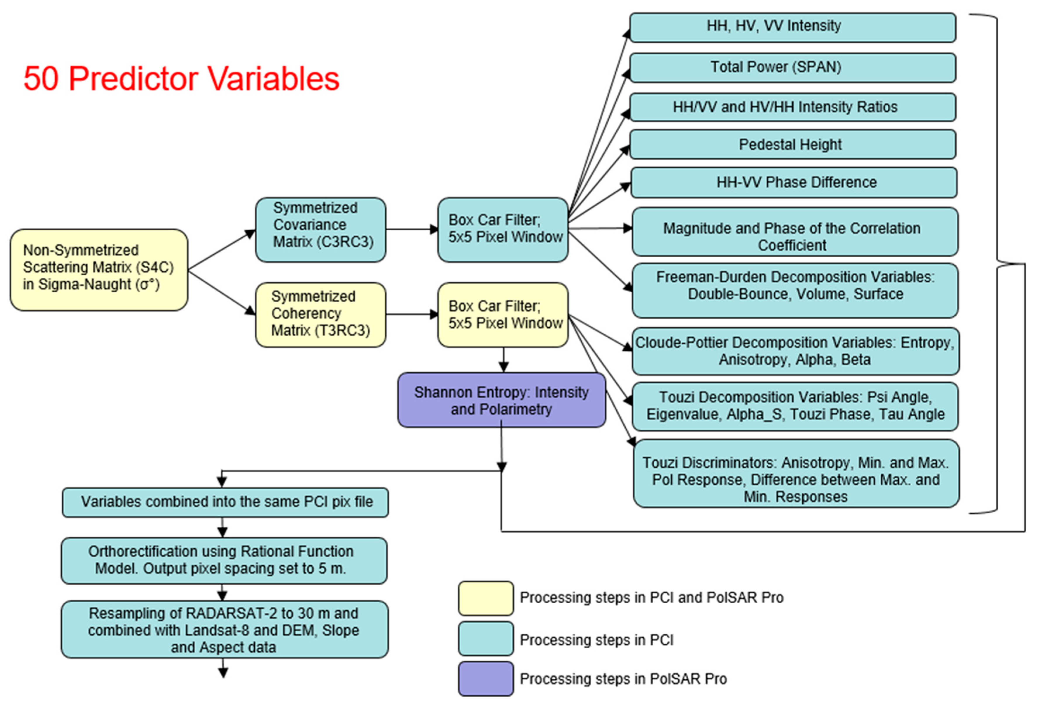
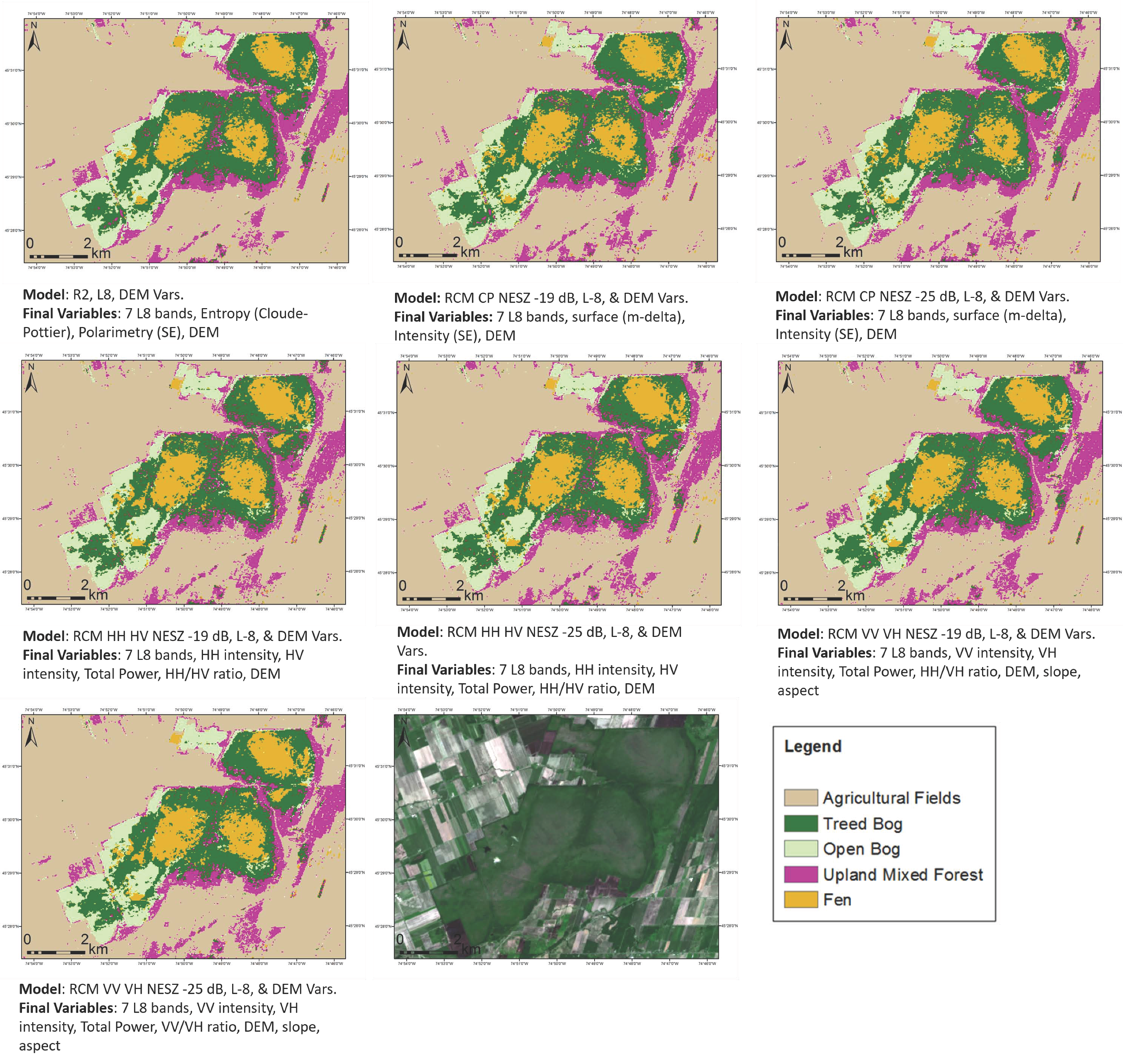
Statistical results from the RADARSAT-2 (2 May 2014), Landsat-8 (24 April 2014), and Shuttle Radar Topographic Mission (SRTM) variables spring model. The first iteration was run with all 50 variables, and variables ranked to be unimportant were then removed until 9 variables remained. The final variables in the model with the highest independent overall accuracy (10 variables) in order of decreasing importance were the seven Landsat-8 bands, Entropy from Claude–Pottier, SRTM DEM, and the polarimetry from the Shannon Entropy.
Number of VariablesOOBE (%)Independent Overall Accuracy (%)Kappa StatisticAgricultural FieldsTreed BogOpen BogUpland Mixed ForestFen
UA (%)PA (%)UA (%)PA (%)UA (%)PA (%)UA (%)PA (%)UA (%)PA (%)
5078830.7895936884947063839077
4578830.7896936883927164839178
4078830.7895926884927163829176
3579820.7795926582917263829172
3080820.7794946583907365789171
2579840.7994956884927668789274
2080840.8094936889947769788974
1580850.8194936990917870818674
1279860.8294927493978069788878
1179850.8193927293968271758874
1080880.8496947492948478829078
977870.8292937593948375749278
Landsat & SRTM variables80820.7684906985977972698674
RADARSAT & SRTM variables59550.4165753764803746649512
Landsat only78790.7387886782937558618174
RADARSAT only49440.295851276069254779364
Table A2. 
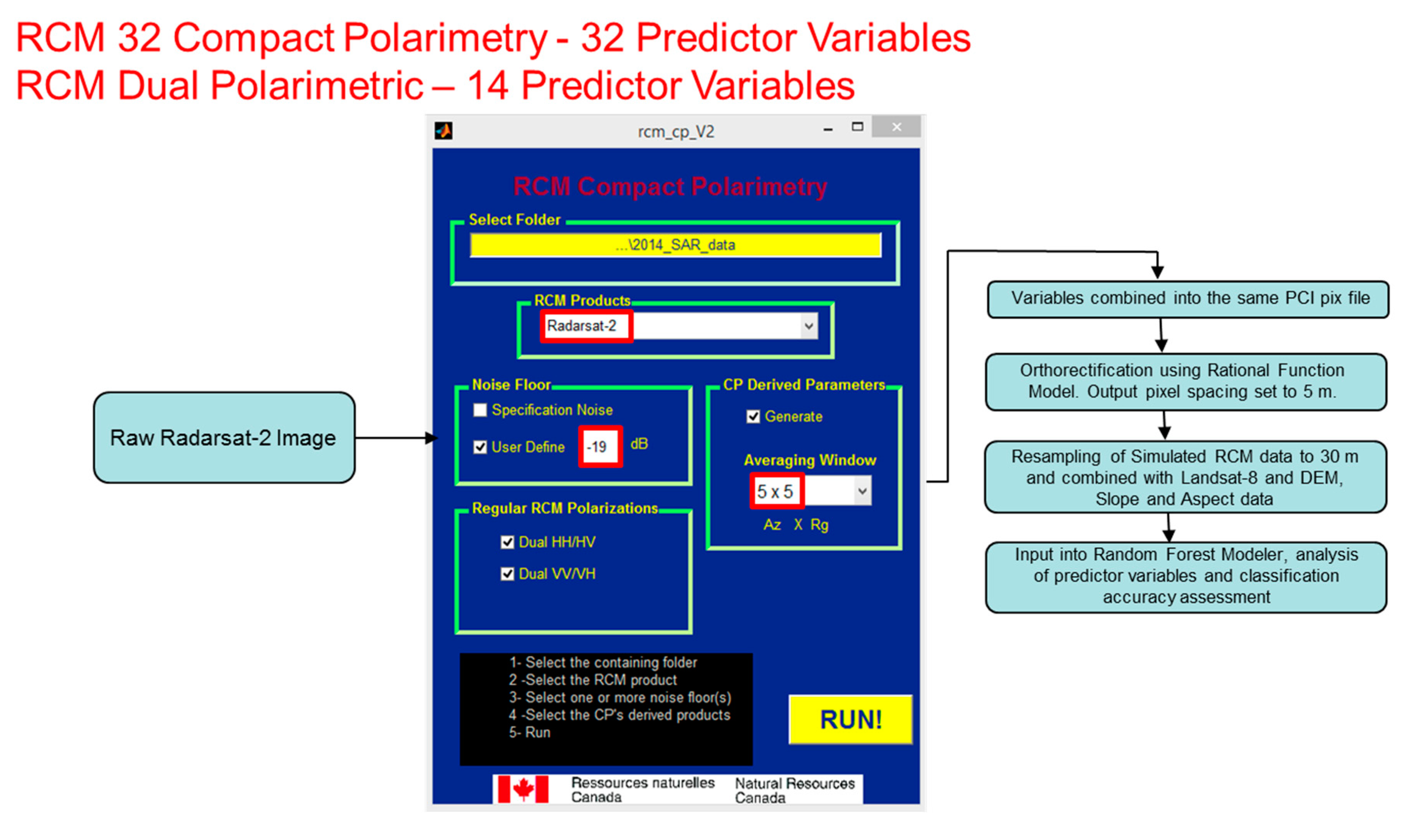
Statistical results from the RCM CP NESZ −19 dB (2 May 2014), Landsat-8 (24 April 2014), and SRTM variables spring model. The first iteration was run with all 50 variables, and variables ranked to be unimportant were then removed until 9 variables remained. The final variables in the model with the highest independent overall accuracy (10 variables) in order of decreasing importance were the seven Landsat-8 bands, m-delta surface, Intensity from Shannon Entropy, and SRTM DEM.
Number of VariablesOOBE (%)Independent Overall Accuracy (%)Kappa StatisticAgricultural FieldsTreed BogOpen BogUpland Mixed ForestFen
UA (%)PA (%)UA (%)PA (%)UA (%)PA (%)UA (%)PA (%)UA (%)PA (%)
3278800.7490906579897160758874
2778800.7487926979907559648674
2279790.7388916679897458668974
1779800.7388906976907555688977
1280820.7691926879927761708678
1180830.7890936979948166708678
1080840.7990937083948170708678
980830.7890936885977867708574
Landsat & SRTM variables80820.7684906985977972698674
RCM CP & SRTM variables60570.4368733851664346716828
Landsat only78790.7390748860646782918574
RCM CP only49390.2350392340613940662514
Table A3. Statistical results from the RCM CP NESZ −25 dB (2 May 2014), Landsat-8 (24 April 2014), and SRTM variables spring model. The first iteration was run with all 50 variables, and variables ranked to be unimportant were then removed until 9 variables remained. The final variables in the model with the highest independent overall accuracy (10 variables) in order of decreasing importance were the seven Landsat-8 bands, m-delta surface, Intensity from Shannon Entropy, and SRTM DEM.
Number of VariablesOOBE (%)Independent Overall Accuracy (%)Kappa StatisticAgricultural FieldsTreed BogOpen BogUpland Mixed ForestFen
UA (%)PA (%)UA (%)PA (%)UA (%)PA (%)UA (%)PA (%)UA (%)PA (%)
3278810.7591916681917164898073
2779810.7589926981927163857473
2279800.7489916879937160857474
1780810.7587906881937662897074
1282820.7790916982937866867477
1179840.7990926982948071877378
1080840.8092926982948173867978
979840.7991936784977975857874
Landsat & SRTM variables80820.7684906985977972698674
RCM CP & SRTM variables58560.4369773656763448607420
Landsat only78790.7390748860646782918574
RCM CP only49380.2153392143552638336913
Table A4. Statistical results from the RCM Dual Pol HH+HV NESZ −19 dB (2 May 2014), Landsat-8 (24 April 2014), and SRTM variables spring model. The first iteration was run with all 14 variables, and variables ranked to be unimportant were then removed until 9 variables remained. The final variables in the model with the highest independent overall accuracy (12 variables) in order of decreasing importance were the seven Landsat-8 bands, HH Intensity, HV Intensity, Total Power, HH/HV ratio, and SRTM DEM.
Number of VariablesOOBE (%)Independent Overall Accuracy (%)Kappa StatisticAgricultural FieldsTreed BogOpen BogUpland Mixed ForestFen
UA (%)PA (%)UA (%)PA (%)UA (%)PA (%)UA (%)PA (%)UA (%)PA (%)
1480830.7889957182958068638177
1382830.7890956982948071658176
1280840.7991946982958068708477
1180830.7789927082978068708077
1080820.7790917083957866687978
979830.7890907483978364718178
Landsat & SRTM variables80820.7684906985977972698674
RCM HH+HV & SRTM variables56550.4167376450557360425824
Landsat only78790.7390748860646782918574
RCM HH+HV only42420.255453314952274160159
Table A5. Statistical results from the RCM Dual Pol HH+HV NESZ −25 dB (2 May 2014), Landsat-8 (24 April 2014), and SRTM variables spring model. The first iteration was run with all 14 variables, and variables ranked to be unimportant were then removed until 9 variables remained. The final variables in the model with the highest independent overall accuracy (13 variables) in order of decreasing importance were the seven Landsat-8 bands, HH Intensity, HV Intensity, Total Power, HH/HV ratio, SRTM DEM, and SRTM slope.
Number of VariablesOOBE (%)Independent Overall Accuracy (%)Kappa StatisticAgricultural FieldsTreed BogOpen BogUpland Mixed ForestFen
UA (%)PA (%)UA (%)PA (%)UA (%)PA (%)UA (%)PA (%)UA (%)PA (%)
1480840.7890967182958170648377
1380840.7990966982948171648477
1280840.7991946982948169708577
1180830.7790926983977968708076
1080820.7791916982957866707877
980830.7889907482978364708277
Landsat & SRTM variables80820.7684906985977972698674
RCM HH+HV & SRTM variables56550.4167733758634249576026
Landsat only78790.7390886482917460678574
RCM HH+HV only41420.2454542945472838552412
Table A6. Statistical results from the RCM Dual Pol VV+VH NESZ −19 dB (2 May 2014), Landsat-8 (24 April 2014), and SRTM variables spring model. The first iteration was run with all 14 variables, and variables ranked to be unimportant were then removed until 9 variables remained. The final variables in the model with the highest independent overall accuracy (14 variables) in order of decreasing importance were the seven Landsat-8 bands, VV Intensity, HV Intensity, Total Power, VV/HV ratio, SRTM DEM, SRTM slope, and SRTM aspect.
Number of VariablesOOBE (%)Independent Overall Accuracy (%)Kappa StatisticAgricultural FieldsTreed BogOpen BogUpland Mixed ForestFen
UA (%)PA (%)UA (%)PA (%)UA (%)PA (%)UA (%)PA (%)UA (%)PA (%)
1478850.8089917786978864678878
1378850.8089937586978665678978
1278840.8089917586978667708977
1179830.7887907386978467678677
1079830.7887907385978369708477
980840.7989907582978469778278
Landsat & SRTM variables80820.7684906985977972698674
RCM VV HV & SRTM variables56600.4868714868674749506051
Landsat only78790.7390886482917460678574
RCM VV HV only40360.1749502245401429354522
Table A7. Statistical results from the RCM Dual Pol VV+VH NESZ −25 dB (2 May 2014), Landsat-8 (24 April 2014), and SRTM variables spring model. The first iteration was run with all 14 variables, and variables ranked to be unimportant were then removed until 9 variables remained. The final variables in the model with the highest independent overall accuracy (14 variables) in order of decreasing importance were the seven Landsat-8 bands, VV Intensity, HV Intensity, Total Power, VV/HV ratio, SRTM DEM, SRTM slope, and SRTM aspect.
Number of VariablesOOBE (%)Independent Overall Accuracy (%)Kappa StatisticAgricultural FieldsTreed BogOpen BogUpland Mixed ForestFen
UA (%)PA (%)UA (%)PA (%)UA (%)PA (%)UA (%)PA (%)UA (%)PA (%)
1478850.8090927686978864698878
1379850.8090927586978665688878
1278850.8089927486978667708977
1179840.7987907486978568688678
1079830.7887907485978468698378
980840.7989907482978470788277
Landsat & SRTM variables80820.7684906985977972698674
RCM VV HV & SRTM variables56600.4867724868674650516352
Landsat only78790.7390886482917460678574
RCM VV HV only40370.1952492245411530395430
Table A8. Statistical results from the RADARSAT-2 (13 July 2014), Landsat-8 (27 June 2014), and SRTM variables spring model. The first iteration was run with all 50 variables, and variables ranked to be unimportant were then removed until 9 variables remained. The final variables in the model with the highest independent overall accuracy (9 variables) in order of decreasing importance were the six Landsat-8 bands, Alpha angle, HH+VV real component of the correlation coefficient, and SRTM DEM).
Number of VariablesOOBE (%)Independent Overall Accuracy (%)Kappa StatisticAgricultural FieldsTreed BogOpen BogUpland Mixed ForestFen
UA (%)PA (%)UA (%)PA (%)UA (%)PA (%)UA (%)PA (%)UA (%)PA (%)
5075760.68779462931004676738157
4574750.75769462931004277748157
4075760.68769563931004378738259
3575760.6876956393994375678564
3074710.6171946189863874657648
2576760.6876936490955172668761
2076770.6976936591945474678863
1577780.7177926790935674708968
1278770.7079936484916176688261
1179770.7078936682906177748261
1078790.7379957083926677748463
974810.7481946986936878768965
Landsat & SRTM variables76760.6977896783836175738764
RADARSAT & SRTM variables51530.3659873350772351345933
Landsat only77750.6777876382835874748061
RADARSAT only37320.10385123475412302920
Table A9. Statistical results from the RCM CP NESZ −19 dB (13 July 2014), Landsat-8 (27 June 2014), SRTM variables summer model. The first iteration was run with all 32 variables, and variables ranked to be unimportant were then removed until 9 variables remained. The final variables in the model with the highest independent overall accuracy (10 variables) in order of decreasing importance were the seven Landsat-8 bands, RV Intensity, Shannon Entropy Intensity, and SRTM DEM.
Number of VariablesOOBE (%)Independent Overall Accuracy (%)Kappa StatisticAgricultural FieldsTreed BogOpen BogUpland Mixed ForestFen
UA (%)PA (%)UA (%)PA (%)UA (%)PA (%)UA (%)PA (%)UA (%)PA (%)
3276730.6476916592804565608361
2778740.6678896491825066638764
2277750.6777906691835370648664
1777750.6777906289845178688365
1276780.7180906588926076758365
1176780.7181906484956371788465
1077780.7180926986836280788261
977780.7180926883826279778261
Landsat & SRTM variables76760.6977896783836175738764
RCM CP & SRTM variables50520.3764784164583033396520
Landsat only77750.6777876382835874748061
RCM CP only35380.184658294161312231214
Table A10. Statistical results from the RCM CP NESZ −25 dB (13 July 2014), Landsat-8 (27 June 2014), SRTM variables summer model. The first iteration was run with all 32 variables, and variables ranked to be unimportant were then removed until 9 variables remained. The final variables in the model with the highest independent overall accuracy (10 variables) in order of decreasing importance were the seven Landsat-8 bands, HV Intensity, Shannon Entropy Intensity, and SRTM DEM.
Number of VariablesOOBE (%)Independent Overall Accuracy (%)Kappa StatisticAgricultural FieldsTreed BogOpen BogUpland Mixed ForestFen
UA (%)PA (%)UA (%)PA (%)UA (%)PA (%)UA (%)PA (%)UA (%)PA (%)
3274750.6874907086865073728168
2775780.7077907186875874758469
2274780.7077907088895774748468
1776770.7077916887905877748063
1276780.7178927085845981757965
1177770.7079926883836181757862
1076790.7381906689966474788765
976790.7281906488946372778965
Landsat & SRTM variables76760.6977896783836175738764
RCM CP & SRTM variables49510.3457763857432352326140
Landsat only77750.6777876382835874748061
RCM CP only28340.1341472143362244294314
Table A11. Statistical results from the RCM Dual Pol HH+HV NESZ −19 dB (13 July 2014), Landsat-8 (27 June 2014), SRTM variables summer model. The first iteration was run with all 14 variables, and variables ranked to be unimportant were then removed until 9 variables remained. The final variables in the model with the highest independent overall accuracy (10 variables) in order of decreasing importance were the seven Landsat-8 bands, HV Intensity, SRTM DEM, and SRTM slope.
Number of VariablesOOBE (%)Independent Overall Accuracy (%)Kappa StatisticAgricultural FieldsTreed BogOpen BogUpland Mixed ForestFen
UA (%)PA (%)UA (%)PA (%)UA (%)PA (%)UA (%)PA (%)UA (%)PA (%)
1475770.7081905887955984797861
1375780.7181905991955884788561
1275780.7181906090935984788461
1175790.7281906293925982788762
1075790.7281906393926181748763
9 (no radar)75790.7382906593916477738865
Landsat & SRTM variables76760.6977896783836175738764
RCM HH+HV & SRTM variables52470.3162703143703325324432
Landsat only77750.6777876382835874748061
RCM HH+HV only31330.1242492735341824312817
Table A12. Statistical results from the RCM Dual Pol HH+HV NESZ −25 dB (13 July 2014), Landsat-8 (27 June 2014), SRTM variables summer model. The first iteration was run with all 14 variables, and variables ranked to be unimportant were then removed until 9 variables remained. The final variables in the model with the highest independent overall accuracy (10 variables) in order of decreasing importance were the seven Landsat-8 bands, HV Intensity, SRTM DEM, and SRTM slope.
Number of VariablesOOBE (%)Independent Overall Accuracy (%)Kappa StatisticAgricultural FieldsTreed BogOpen BogUpland Mixed ForestFen
UA (%)PA (%)UA (%)PA (%)UA (%)PA (%)UA (%)PA (%)UA (%)PA (%)
1474770.7081905985965881797661
1375770.7081905988945980768361
1275780.7181906091935884788461
1175790.7281906291926081788663
1075790.7281906493926178748864
9 (no radar)75790.7382906593916477738865
Landsat & SRTM variables76760.6977896783836175738764
RCM HH+HV & SRTM variables54490.3363713240653628364434
Landsat only77750.6777876382835874748061
RCM HH+HV only29350.1344562332472323251910
Table A13. Statistical results from the RCM Dual Pol VV+VH NESZ −19 dB (13 July 2014), Landsat-8 (27 June 2014), SRTM variables summer model. The first iteration was run with all 14 variables, and variables ranked to be unimportant were then removed until 9 variables remained. The final variables in the model with the highest independent overall accuracy (10 variables) in order of decreasing importance were the seven Landsat-8 bands, HV Intensity, SRTM DEM, and SRTM slope.
Number of VariablesOOBE (%)Independent Overall Accuracy (%)Kappa StatisticAgricultural FieldsTreed BogOpen BogUpland Mixed ForestFen
UA (%)PA (%)UA (%)PA (%)UA (%)PA (%)UA (%)PA (%)UA (%)PA (%)
1474780.7182906186926280747965
1375780.7182906189926376748261
1275780.7283906290926377748363
1175780.7181906290926179748362
1075790.7281906393926181748763
976780.7182906388926170748965
Landsat & SRTM variables76760.6977896783836175738764
RCM VV HV & SRTM variables51530.3868783655593735284332
Landsat only77750.6777876382835874748061
RCM HH+HV only31360.1645512750531920183625
Table A14. Statistical results from the RCM Dual Pol VV+VH NESZ −25 dB (13 July 2014), Landsat-8 (27 June 2014), SRTM variables summer model. The first iteration was run with all 14 variables, and variables ranked to be unimportant were then removed until 9 variables remained. The final variables in the model with the highest independent overall accuracy (10 variables) in order of decreasing importance were the seven Landsat-8 bands, HV Intensity, SRTM DEM, and SRTM slope.
Number of VariablesOOBE (%)Independent Overall Accuracy (%)Kappa StatisticAgricultural FieldsTreed BogOpen BogUpland Mixed ForestFen
UA (%)PA (%)UA (%)PA (%)UA (%)PA (%)UA (%)PA (%)UA (%)PA (%)
1475790.7277936890955983748463
1375780.7177936891955880748761
1276790.7277936891966081748761
1176790.7278936890966380748461
1077810.7480936989967081748261
976790.7380926882967174737962
Landsat & SRTM variables76760.6977896783836175738764
RCM VV HV & SRTM variables51520.3561803951623033254738
Landsat only77750.6777876382835874748061
RCM HH+HV only31310.1142402244601819222118

References

  1. Food and Agriculture Organization of the United Nations. Mitigation of Climate Change in Agriculture (MICCA) Programme. Available online: http://www.fao.org/in-action/micca/knowledge/peatlands-and-organic-soils/en/ (accessed on 3 August 2016).
  2. Tarnocai, C. The Impact of climate Change on Canadian Peatlands. Can. Water Resour. J. 2009, 34, 453–466. [Google Scholar] [CrossRef]
  3. Cox, D.D. A Naturalists Guide to Wetlands Plants: An Ecology for Eastern North America, 1st ed.; Syracuse University Press: New York, NY, USA, 2002; pp. 1–194. [Google Scholar]
  4. International Peatland Society. What Is Peat? Available online: http://www.peatsociety.org/peatlands-and-peat/what-peat (accessed on 1 August 2016).
  5. Joosten, H.; Clarke, D. Wise Use of Mires and Peatlands—Background and Principles Including a Framework for Decision-Making; International Mire Conservation Group/International Peat Society: Totnes, UK, 2002; pp. 10–253. [Google Scholar]
  6. Runkle, B.R.K.; Kutzbach, B. Peatland Characterization. In Towards Climate-Responsible Peatlands Management; Biancalani, R., Avagyan, A., Eds.; Food and Agriculture Organization of the United Nations (FAO): Rome, Italy, 2014; pp. 6–32. [Google Scholar]
  7. Riordan, R.; Verbyla, D.; McGuire, A.D. Shrinking ponds in subarctic Alaska based on 1950–2002 remotely sensed images. J. Geophys. Res. 2006, 111, G04002. [Google Scholar] [CrossRef]
  8. Ozesmi, S.L.; Bauer, M.E. Satellite remote sensing of wetlands. Wetl. Ecol. Manag. 2002, 10, 381–402. [Google Scholar] [CrossRef]
  9. National Round Table on the Environment and the Economy. Available online: http://collectionscanada.gc.ca/webarchives2/20130322182509/http://nrtee-trnee.ca/wp-content/uploads/2013/02/environment-sustainable-development-indicators.pdf (accessed on 6 July 2016).
  10. Gilmer, D.S.; Work, E.A., Jr.; Colwell, J.E.; Rebel, D.L. Enumeration of prairie wetlands with Landsat and aircraft data. Photogramm. Eng. Remote Sens. 1980, 46, 631–634. [Google Scholar]
  11. Haack, B. Environmental auditing: Monitoring wetland changes with remote sensing: An east African example. Environ. Manag. 1996, 20, 411–419. [Google Scholar] [CrossRef]
  12. Gross, M.F.; Hardisky, M.A.; Klemas, V.; Wolf, P.L. Quantification of biomass of the marsh grass Spartina alterniflora Louisel using Landsat Thematic Mapper imagery. Photogramm. Eng. Remote Sens. 1987, 53, 1577–1583. [Google Scholar]
  13. Houhoulis, P.F.; Michener, W.K. Detecting wetland change: A rule-based approach using NWI and SPOT-XS data. Photogramm. Eng. Remote Sens. 2000, 66, 205–211. [Google Scholar]
  14. Laine, B.B.; Naslund-Landenmark, B. Wetland classification for Swedish CORINE Land cover adopting a semi-automatic interactive approach. Can. J. Remote Sens. 2002, 28, 139–155. [Google Scholar]
  15. Sader, S.A.; Ahl, D.; Liou, W. Accuracy of Landsat-TM and GIS rule-based methods for forested wetland classification in Maine. Remote Sens. Environ. 1995, 53, 133–144. [Google Scholar] [CrossRef]
  16. Lozano-Garcia, D.F.; Hoffer, R.M. Synergistic effects of combined Landsat-TM and SI R-B data for forest resources assessment. Int. J. Remote Sens. 1993, 14, 2677–2694. [Google Scholar] [CrossRef]
  17. Toyra, J.; Pietroniro, A.; Martz, L. Multisensor hydrologica assessment of freshwater wetland. Remote Sens. Environ. 2001, 75, 162–173. [Google Scholar] [CrossRef]
  18. Bourgeau-Chavez, L.L.; Riordan, K.; Nowels, M.; Miller, N. Final Report to the Great Lakes Commission: Remotely Monitoring Great Lakes Coastal Wetlands Using a Hybrid Radar and Multi-Spectral Sensor Approach; Project No. WETLANDS2-WPA-06. 82; Great Lakes Commission: Ann Arbor, MI, USA, 2004. [Google Scholar]
  19. Bourgeau-Chavez, L.L.; Lopez, R.D.; Trebitz, A.; Hollenhorst, T.; Host, G.E.; Huberty, B.; Gauthier, R.L.; Hummer, J. Chapter 8: Landscape-based indicators. In Great Lakes Coastal Wetlands Monitoring Plan; Great Lakes Coastal Wetlands Consortium, Project of the Great Lakes Commission: Ann Arbor, MI, USA, 2008; pp. 143–171. [Google Scholar]
  20. Bourgeau-Chavez, L.L.; Riordan, K.; Powell, R.B.; Miller, N.; Nowels, M. Improving Wetland Characterization with Multi-Sensor, Multi-Temporal SAR and Optical/Infrared Data Fusion, Advances. In Geoscience and Remote Sensing; Jedlovec, G., Ed.; InTech: Exton, PA, USA, 2009; Available online: http://www.intechopen.com/books/advances-in-geoscience-and-remote-sensing/improving-wetland-characterization-with-multi-sensor-multi-temporal-sar-and-optical-infrared-data-fu (accessed on 1 June 2016).
  21. Grenier, M.; DEMers, A.; Labrecque, M.S.; Benoit, M.; Fournier, R.A. An object-based method to map wetland using RADARSAT-1 and Landsat-ETM images: Test case on two sites in Quebec Canada. Can. J. Remote Sens. 2007, 33, 528–545. [Google Scholar] [CrossRef]
  22. Li, J.; Chen, W. A rule-based method for mapping Canada’s wetlands using optical, radar and DEM data. Int. J. Remote Sens. 2005, 26, 5051–5069. [Google Scholar] [CrossRef]
  23. Lang, M.W.; Kasischke, E.S. Using C-Band Synthetic Aperture Radar Data to Monitor Forested Wetland Hydrology in Maryland’s Coastal Plain, USA. IEEE Trans. Geosci. Remote Sens. 2008, 46, 535–546. [Google Scholar] [CrossRef]
  24. Dobson, M.C.; Ulaby, F.T. Active Microwave Soil Moisture Research. IEEE Trans. Geosci. Remote Sens. 1988, 24, 23–36. [Google Scholar] [CrossRef]
  25. Brisco, B.; Kapfer, M.; Hirose, T.; Tedford, B.; Liu, J. Evaluation of C-band polarization diversity and polarimetry for wetland mapping. Can. J. Remote Sens. 2011, 37, 82–92. [Google Scholar] [CrossRef]
  26. Brisco, B.; Li, K.; Tedford, B.; Charbonneau, F.; Yun, S.; Murnaghan, K. Compact polarimetry assessment for rice and wetland mapping. Int. J. Remote Sens. 2013, 34, 1949–1964. [Google Scholar] [CrossRef]
  27. Brisco, B.; Touzi, R.; van der Sanden, J.J.; Charbonneau, F.; Pultz, T.J.; D’Iorio, M. Water resource applications with RADARSAT-2—A preview. Int. J. Digit. Earth 2008, 1, 130–147. [Google Scholar] [CrossRef]
  28. Hess, L.; Melack, J.; Novo, E.; Barbosa, C.; Gastil, M. Dual season mapping of wetland inundation and vegetation for the central Amazon Basin. Remote Sens. Environ. 2003, 87, 404–428. [Google Scholar] [CrossRef]
  29. Lane, C.R.; D’Amico, E. Calculating the ecosystem service of water storage in isolated wetlands using LiDAR in North Central Florida, United States. Wetlands 2010, 30, 967–977. [Google Scholar] [CrossRef]
  30. Wdowinski, S.; Kim, S.W.; Amelung, F.; Dixon, T.H.; Miralles-Wilhelm, F.; Sonenshein, R. Space-based detection of wetlands’ surface water level changes from L band SAR interferometry. Remote Sens. Environ. 2008, 112, 681–696. [Google Scholar] [CrossRef]
  31. Marechal, C.; Pottier, E.; Hubert-Moy, L.; Rapinel, S. One year wetland survey investigations from quad-pol RADARSAT-2 time-series SAR images. Can. J. Remote Sens. 2012, 38, 240–252. [Google Scholar] [CrossRef]
  32. Gosselin, G.; Touzi, R.; Cavayas, F. Polarimetric RADARSAT-2 wetland classification using the Touzi decomposition: Case of the Lac Saint-Pierre Ramsar wetland. Can. J. Remote Sens. 2014, 39, 491–506. [Google Scholar] [CrossRef]
  33. White, L.; Brisco, B.; Dabboor, M.; Schmitt, A.; Pratt, A. A Collection of SAR Methodologies for Monitoring Wetlands. Remote Sens. 2015, 7, 7615–7645. [Google Scholar] [CrossRef]
  34. Thompson, A. Overview of the RADARSAT Constellation Mission. Can. J. Remote Sens. 2015, 41, 401–407. [Google Scholar] [CrossRef]
  35. Canadian Space Agency. RADARSAT Constellation. Available online: http://www.asc-csa.gc.ca/eng/satellites/RADARSAT/ (accessed on 17 August 2016).
  36. Brisco, B.; Ahern, F.; Murnaghan, K.; White, L.; Canisus, F.; Lancaster, F. Seasonal Change in Wetland Coherence as an Aid to Wetland Monitoring. Remote Sens. 2017, 9. [Google Scholar] [CrossRef]
  37. Raney, R.K. Hybrid-polarity SAR architecture. IEEE Trans. Geosci. Remote Sens. 2007, 45, 3397–3404. [Google Scholar] [CrossRef]
  38. Charbonneau, F.J.; Brisco, B.; Raney, R.K.; McNairn, H.; Liu, C.; Vachon, P.W.; Shang, J.; DeAbreu, R.; Champagne, C.; Merzouki, A.; et al. Compact polarimetry overview and applications assessment. Can. J. Remote Sens. 2010, 36, 298–315. [Google Scholar] [CrossRef]
  39. Corcoran, J.; Knight, J.; Gallant, A. Influence of multi-source and multi-temporal remotely sensed and ancillary data on the accuracy of random forest classification of wetlands in Northern Minnesota. Remote Sens. 2013, 5, 3212–3238. [Google Scholar] [CrossRef]
  40. Millard, K.; Richardson, M. Wetland mapping with LiDAR derivatives, SAR polarimetric decompositions, and LiDAR-SAR fusion using a random forest classifier. Can. J. Remote Sens. 2013, 39, 290–307. [Google Scholar] [CrossRef]
  41. Van Beijma, S.; Comber, A.; Lamb, A. Random forest classification of salt marsh vegetation habitats using quad-polarimetric airborne SAR, elevation and optical RS data. Remote Sens. Environ. 2014, 149, 118–129. [Google Scholar] [CrossRef]
  42. Breiman, L. Random Forests. Mach. Learn. 2001, 45, 5–32. [Google Scholar] [CrossRef]
  43. Prasad, A.; Iverson, L.; Liaw, A. Newer classification and regression tree techniques: Bagging and random forests for ecological prediction. Ecosystems 2006, 9, 181–199. [Google Scholar] [CrossRef]
  44. Liaw, A.; Wiener, M. Classification and regression by randomForest. R News 2002, 2, 18–22. [Google Scholar]
  45. Waske, B.; Braun, M. Classifier ensembles for land cover mapping using multi-temporal SAR imagery. ISPRS J. Photogramm. Remote Sens. 2009, 64, 450–457. [Google Scholar] [CrossRef]
  46. Ghimire, B.; Rogan, J.; Miller, J. Contextual land-cover classification: Incorporating spatial dependence in land-cover classification models using random forests and the Ghetis statistic. Remote Sens. Lett. 2010, 1, 45–54. [Google Scholar] [CrossRef]
  47. Dietterich, T.G. Ensemble methods in machine learning. In Multiple Classifier Systems; Lecture Notes in Computer Science; Springer: Berlin/Heidelberg, Germany, 2000; pp. 1–15. [Google Scholar]
  48. Kotsiantis, S.B.; Pintelas, P.E. Combining bagging and boosting. Int. J. Comp. Intell. 2004, 1, 324–333. [Google Scholar]
  49. Millard, K.; Richardson, M. On the importance of training data sample selection in random forest image classification: A case study in peatland ecosystem mapping. Remote Sens. 2015, 7, 8489–8515. [Google Scholar] [CrossRef]
  50. Banks, S.; Millard, K.; Pasher, J.; Richardson, M.; Wang, H.; Duffe, J. Assessing the Potential to Operationalize Shoreline Sensitivity Mapping: Classifying Multiple Wide Fine Quadrature Polarized RADARSAT-2 and Landsat 5 Scenes with a Single Random Forest Model. Remote Sens. 2015, 7, 13528–13563. [Google Scholar] [CrossRef]
  51. Horning, N. Random forests: An algorithm for image classification and generation of continuous fields data sets. In Proceedings of the International Conference on Geoinformatics for Spatial Infrastructure Development in Earth and Allied Sciences, Osaka, Japan, 9–11 December 2010. [Google Scholar]
  52. Gislason, P.O.; Benediktsson, J.A.; Sveinsson, J.R. Random forests for land cover classification. Pattern Recogn. Lett. 2006, 27, 294–300. [Google Scholar] [CrossRef]
  53. Loosvelt, L.; Peters, J.; Skriver, H.; Lievens, H.; Van Coillie, F.; De Baets, B.; Verhoest, N.E.C. Random forests as a tool for estimating uncertainty at pixel-level in SAR image classification. Int. J. Appl. Earth Obs. 2012, 19, 173–184. [Google Scholar] [CrossRef]
  54. Sonobe, R.; Tani, H.; Wang, X.; Kobayashi, N.; Shimamura, H. Random forest classification of crop type using multi-temporal TerraSAR-X dual-polarimetric data. Remote Sens. Lett. 2014, 5, 157–164. [Google Scholar] [CrossRef]
  55. The Ottawa Field-Naturalists’ Club—The Alfred Bog. Available online: http://ofnc.ca/conservation/alfredBog/index.php (accessed on 8 August 2016).
  56. Millard, K. Development of Methods to Map and Monitor Peatland Ecosystems and Hydrologic Conditions Using Radarsat-2 Synthetic Aperture Radar. Ph.D. Thesis, Carleton University, Department of Geography and Environmental Studies, Ottawa, ON, Canada, 2016. [Google Scholar]
  57. USGS Earth Explorer. Available online: http://earthexplorer.usgs.gov/ (accessed on 16 February 2016).
  58. Department of the Interior U.S. Geological Survey. Product Guide Landsat 8 Surface Reflectance Code (LaSRC). Available online: https://landsat.usgs.gov/sites/default/files/documents/lasrc_product_guide.pdf (accessed on 16 February 2016).
  59. Chamberlain, D.; Tighe, M.L. Land Cover Classification: A Comparison Between U.S. National Land Cover Dataset (NLCD) and Intermap’s NEXTMAP® USA Derived Land Cover Maps. In Proceedings of the ASPRS/MAPPS Fall Conference, San Antonio, TX, USA, 16–19 November 2009. [Google Scholar]
  60. Hijmans, R. Raster: Geographic Data Analysis and Modeling, R Package Version 2.3. Available online: https://cran.r-project.org/web/packages/raster/raster.pdf (accessed on 6 June 2016).
  61. Foody, G. Thematic Map comparison: Evaluating the statistical significance of differences in classification accuracy. Photogramm. Eng. Remote Sens. 2004, 70, 627–633. [Google Scholar] [CrossRef]
  62. Dietterich, T. Approximate statistical tests for comparing supervised classification learning algorithms. Neural Comput. 1998, 10, 1895–1923. [Google Scholar] [CrossRef] [PubMed]
  63. Bradley, J.V. Distribution-Free Statistical Tests; Prentice-Hall: Englewood Cliffs, NJ, USA, 1968; p. 388. [Google Scholar]
  64. Agresti, A. An Introduction to Categorical Data Analysis; Wiley: New York, NY, USA, 1996; p. 312. [Google Scholar]
  65. Younis, M. General Formulation of NESZ; Technical Note TN-SAR-Tech-001; Microwaves and Radar Institute, German Aerospace Center: Wessling, Germany, 2008. [Google Scholar]
  66. Baghdadi, N.; Bernier, M.; Gauthier, R.; Neeson, I. Evaluation of C-band SAR data for wetlands mapping. Int. J. Remote Sens. 2001, 22, 71–88. [Google Scholar] [CrossRef]
  67. Dingle Robertson, L. Evaluating Spatial and Seasonal Variability of Wetlands in Eastern Ontario Using Remote Sensing and GIS. Ph.D. Thesis, Carleton University, Ottawa, ON, Canada, 2014. [Google Scholar]
  68. Pope, K.O.; Rejmankova, E.; Paris, J.F.; Woodruff, R. Detecting seasonal flooding cycles in marches of the Yucatan Peninsula with SIR-C polarimetric radar imagery. Remote Sens. Environ. 1997, 59, 157–166. [Google Scholar] [CrossRef]
  69. Parmuchi, G.G.; Karszenbaum, H.; Kandus, P. Mapping wetlands using multi-temporal RADARSAT-1 data and a decision-based classifier. Can. J. Remote Sens. 2002, 28, 175–186. [Google Scholar] [CrossRef]
  70. Costa, M.; Novo, F.; Ahern, E.; Mitsou, E.II.; Mantovani, J.; Allester, M.; Pietsch, R. The Amazon flood plain through radar eyes: Lago Grande de Monte Alegre case study. Can. J. Remote Sens. 1998, 24, 339–349. [Google Scholar] [CrossRef]
  71. Novo, E.M.; Costa, M.F.; Mantovani, J.; Lima, I. Relationship between macrophyte stand variables and radar backscatter at L and C band, Tucuruí Reservoir, Brazil. Int. J. Remote Sens. 2002, 23, 1241–1260. [Google Scholar] [CrossRef]
  72. Kandus, P.; Karsenbaum, H.; Pultz, T.; Parmuchi, G.; Bava, J. Influence of flood conditions and vegetation status on the radar backscatter of wetland ecosystems. Can. J. Remote Sens. 2001, 27, 651–662. [Google Scholar] [CrossRef]
  73. Lang, M.W.; Townsend, P.A.; Kasischke, E.S. Influence of incidence angle on detecting flooded forests using C-HH synthetic aperture radar data. Remote Sens. Environ. 2008, 112, 3898–3907. [Google Scholar] [CrossRef]
  74. Merchant, M. Examining the Influence of Subarctic Boreal Ground Conditions on C-Band Radarst-2 Polsar Variables for Target Separability and the Application of a Support Vector Machine Classifier. Master’s Thesis, University of Guelph, Guelph, ON, Canada, 2014. [Google Scholar]
  75. Martin, J. Mapping Wetlands Areas on Forested Landscapes Using RADSARSAT-2 and Landsat-5 TM Data. Master’s Thesis, University of New Brunswick, Fredericton, NB, Canada, Saint John, NB, Canada, 2012. [Google Scholar]
  76. Dingle Robertson, L.; King, D.J.; Davies, C. Object-based image analysis of optical and radar variables for wetland evaluation. Int. J. Remote Sens. 2015, 36, 5811–5841. [Google Scholar] [CrossRef]
  77. Lee, J.S.; Pottier, E. Polarimetric Radar Imaging: From Basics to Applications; CRC Press, Taylor & Francis: Boca Raton, FL, USA, 2009; p. 397. [Google Scholar]
  78. Betbeder, J.; Rapinel, S.; Corpetti, T.; Pottier, E.; Corgne, S.; Hubert-Moy, L. Multi-temporal classification of TerraSAR-X data for wetland vegetation mapping. J. Appl. Remote Sens. 2014, 8. [Google Scholar] [CrossRef]
  79. Chen, Y.; He, X.; Wang, J.; Xiao, R. The influence of polarimetric parameters and an object-based approach on land cover classification in coastal wetlands. Remote Sens. 2014, 6, 12575–12592. [Google Scholar] [CrossRef]
  80. Betbeder, J.; Rapinel, S.; Corgne, S.; Pottier, E.; Hubert-Moy, L. TerraSAR-X dual-pol time-series for mapping of wetland vegetation. ISPRS J. Photogramm. Remote Sens. 2015, 107, 90–98. [Google Scholar] [CrossRef]
  81. Touzi, R.; Boerner, W.M.; Lee, J.S.; Luneburg, E. A Review of Polarimetry in the Context of Synthetic Aperture Radar: Concepts and Information Extraction. Can. J. Remote Sens. 2004, 30, 380–407. [Google Scholar] [CrossRef]
  82. McNairn, H.; Duguay, C.; Brisco, B.; Pultz, T.J. The Effect of soil and Crop Residue Characteristics on Polarimetric Radar Response. Rem. Sens. Environ. 2002, 80, 308–320. [Google Scholar] [CrossRef]
  83. Boerner, W.M.; Mott, H.; Luneburg, E.; Livingstone, C.; Brisco, B.; Brown, R.J.; Paterson, J.S. Polarimetry in Radar Remote sensing: Basic and Applied Concepts. In Principles and Applications of Imaging Radar: Manual of Remote Sensing; Henderson, R.M., Lewis, A.J., Eds.; John Wiley & Sons: New York, NY, USA, 1998; Volume 2, pp. 271–357. [Google Scholar]
Figure 1. Location map of Alfred Bog [56]. The map in the top left shows Alfred Bog (red star) in relation to the rest of Canada. The lower map is a zoomed in view of Eastern Ontario, and the extent of Alfred Bog is shown as a green polygon to the east. Alfred Bog is located approximately 70 km from the well-known RAMSAR Mer Bleue bog, shown as a green polygon to the west. Mer Bleue and Alfred Bog have very similar land cover classes.
Remotesensing 09 00573 g001
Figure 2. Predictor variables that were included in the Random Forest (RF) models.
Remotesensing 09 00573 g002
Figure 3. Processing steps used in PCI Geomatica 2015 and PolSAR Pro to generate the 50 predictor variables that were used in the RADARSAT-2 RF model (recreated after [50]).
Remotesensing 09 00573 g003
Figure 4. A sample of the processing steps used in the RCM simulator software to produce the predictor variables in the simulated RCM RF models. For the dual pol models 14 predictor variables were available, while for the compact polarimetry (CP) models 32 were available. The simulator was run once with a noise equivalent sigma zero (NESZ) of −19 dB and a second time with a NESZ of −25 dB.
Remotesensing 09 00573 g004
Figure 5. Visual results of the spring RF classifications. Models presented here were those with highest overall independent accuracy after variable reduction. A Landsat-8 image from 27 June 2014 was included for comparison.
Remotesensing 09 00573 g005
Figure 6. Classification results from the summer RF classifications. Models presented here were those with the highest overall independent accuracy after variable reduction. A Landsat-8 image from 27 June 2014 was included for comparison.
Remotesensing 09 00573 g006
Table 1. A description of the RADARSAT Constellation Mission (RCM) imaging mode parameters [29].
Imaging ModePolarization OptionsResolution (m) (Range and Azimuth)Number of Looks (Range and Azimuth)NESZ (dB)Image Swath Width (km)Accessible Swath Width (km)
Low resolution 100 mSingle Pol, Dual Pol (HH+HV, VV+VH, HH+VV), CP100 × 1008 × 1−22500500
Low noiseSingle Pol, Dual Pol (HH+HV, VV+VH), CP100 × 1004 × 2−25350500
Medium Resolution 50 mSingle Pol, Dual Pol (HH+HV, VV+VH, HH+VV), CP50 × 504 × 1−22350500
Medium Resolution 30 mSingle Pol, Dual Pol (HH+HV, VV+VH, HH+VV), CP30 × 302 × 2−24125350
Medium Resolution 16 mSingle Pol, Dual Pol (HH+HV, VV+VH, HH+VV), CP16 × 161 × 4−2530250
High Resolution 5 mSingle Pol, Dual Pol (HH+HV, VV+VH, HH+VV), CP5 × 51 × 1−1930500
Very High Resolution 3 mSingle Pol, Dual Pol (HH+HV, VV+VH, HH+VV), CP3 × 31 × 1−1720500
SpotlightSingle Pol, Dual Pol (HH+HV, VV+VH), CP3 × 11 × 1−17Spot size 5 × 5350
Quad-PolQuad Pol9 × 91 × 1−2420250
Ship DetectionSingle Pol, Dual Pol (HH+HV, VV+VH), CPVariableVariableVariable350600
Table 2. Name of the Landsat-8 bands, their wavelength and resolution that we included in the RF models.
Landsat-8 BandWavelength (Micrometers)Resolution (Meters)
Band 1—Coastal aerosol0.43–0.4530
Band 2—Blue0.45–0.5130
Band 3—Green0.53–0.5930
Band 4—Red0.64–0.6730
Band 5—Near Infrared (NIR)0.85–0.8830
Band 6—SWIR 11.57–1.6530
Band 7—SWIR 22.11–2.2930
Table 3. Combinations of variables used in the RF mapping of landcover within peatlands. Each of the 14 models was first run using a spring RADARSAT-2, simulated RCM, and/or Landsat-8 image. All models were re-run using a summer RADARSAT-2, simulated RCM, and/or Landssat-8 image. For models that used simulated RCM data as predictor variables the models were first run with a NESZ of −19 dB, and a second time with a NESZ of −25 dB.
Variables Used in Random Forest Models
RADARSAT-2, Landsat-8, DEM, Slope, and Aspect
Simulated RCM CP, Landsat-8, DEM, Slope, and Aspect
Simulated RCM HH+HV, Landsat-8, DEM, Slope, and Aspect
Simulated RCM VV+VH, Landsat-8, DEM, Slope, and Aspect
RADARSAT-2, DEM, Slope, and Aspect
Simulated RCM CP, DEM, Slope, and Aspect
Simulated RCM HH+HV, DEM, Slope, and Aspect
Simulated RCM VV+VH, DEM, Slope, and Aspect
Landsat-8, DEM, Slope, and Aspect
Radarsat-2 only
Simulated RCM CP only
Simulated RCM HH+HV only
Simulated RCM VV+VH only
Landsat-8 only
Table 4. Out of bag error (OOBE), Independent Overall Accuracy, Kappa Statistic, and per-class UA and PA or the spring and summer RADARSAT-2 and simulated RCM RF models with the highest Independent Overall Accuracy after variable reduction. All Random Forest models were a combination of either RADARSAT-2 or simulated RCM data, Landsat-8, and SRTM DEM variables.
RF ModelNumber of VariablesOOBE (%)Independent Overall Accuracy (%)Kappa StatisticAgricultural FieldsTreed BogOpen BogUpland Mixed ForestFen
UA (%)PA (%)UA (%)PA (%)UA (%)PA (%)UA (%)PA (%)UA (%)PA (%)
Spring Imagery: 2 May 2014—RADARSAT-2, 24 April 2014—Landsat-8
R21080880.8496947492948478829078
RCM CP NF − 191080840.7990937083948170708678
RCM CP NF − 251080840.8092926982948173798678
RCM HH+HV NF − 191280840.7991946982958068708477
RCM HH+HV NF − 251380840.7990966982948171648477
RCM VV+VH NF − 191478850.8089917786978864678878
RCM VV+VH NF − 251478850.8090927686978864698878
Summer Imagery: 13 July 2014—RADARSAT-2, 27 June 2014—Landsat-8
R2974810.7481946986936878768965
RCM CP NF − 191077780.7180926986836280788261
RCM CP NF − 251076790.7381906689966474788765
RCM HH+HV NF − 191075790.7281906393926181748763
RCM HH+HV NF − 251075790.7281906493926178748864
RCM VV+VH NF − 191075790.7281906393926181748763
RCM VV+VH NF − 251077810.7480936989967081748261
Table 5. p-values from the McNemar test statistic that was used to compare the RADARSAT-2 and simulated RCM Random Forest models with the highest independent overall accuracy. All models were not statistically different (p-values > 0.05) at the 95% confidence level. All RF models were a combination of either RADARSAT-2 or simulated RCM data, Landsat-8, and SRTM DEM variables. The final variables in the model are listed in the appendix. The same validation points used to calculate the independent overall accuracy were used in the McNemar test.
RF Model 1RF Model 2p-Value—Spring RF Modelp-Value—Summer RF Model
R2RCM CP NF − 190.670.16
R2RCM CP NF − 250.390.99
R2RCM HH+HV NF − 190.410.41
R2RCM HH+HV NF − 250.470.56
R2RCM VV+VH NF − 190.200.41
R2RCM VV+VH NF − 250.810.80
RCM CP NF − 19RCM CP NF − 250.410.29
RCM CP NF − 19RCM HH+HV NF − 190.830.80
RCM CP NF − 19RCM HH+HV NF − 250.230.59
RCM CP NF − 19RCM VV+VH NF − 190.440.80
RCM CP NF − 19RCM VV+VH NF − 250.800.37
RCM CP NF − 25RCM HH+HV NF − 190.850.26
RCM CP NF − 25RCM HH+HV NF − 250.110.41
RCM CP NF − 25RCM VV+VH NF − 190.830.26
RCM CP NF − 25RCM VV+VH NF − 250.470.80
RCM HH+HV NF − 19RCM HH+HV NF − 250.180.32
RCM HH+HV NF − 19RCM VV+VH NF − 190.530.99
RCM HH+HV NF − 19RCM VV+VH NF − 250.640.59
RCM HH+HV NF − 25RCM VV+VH NF − 190.180.32
RCM HH+HV NF − 25RCM VV+VH NF − 250.320.78
RCM VV+VH NF − 19RCM VV+VH NF − 250.250.59

