Article

Characterizing the Growth Patterns of 45 Major Metropolitans in Mainland China Using DMSP/OLS Data

1
School of Remote Sensing and Information Engineering, Wuhan University, Wuhan 430072, China
2
Department of Land Surveying and Geo-Informatics, The Hong Kong Polytechnic University, Hong Kong, China
3
Department of Information and Communication, State Grid Corporation of China, Beijing 100031, China
*
Author to whom correspondence should be addressed.
Remote Sens. 2017, 9(6), 571; https://doi.org/10.3390/rs9060571
Submission received: 12 April 2017 / Revised: 25 May 2017 / Accepted: 4 June 2017 / Published: 7 June 2017
(This article belongs to the Special Issue Recent Advances in Remote Sensing with Nighttime Lights)

Abstract

:
Understanding growth patterns at the metropolitan level is instructive for better planning and policy making on sustainable urban development. Using DMSP/OLS data from 1992 to 2013, this article aims to investigate growth patterns of major metropolitans in Mainland China from the aspects of intensification and expansion. We start by calibrating the DMSP/OLS data and selecting 45 major metropolitans. On intensification, results suggest that aggregately, metropolitans displayed cyclical pattern over time and large metropolitans tended to have higher levels of intensification than moderate or small ones. Individually, metropolitans with similar intensification over time could be clustered together using Dendrogram, and evolution pattern of the clusters exhibited similarity to the aggregated one. On expansion, results show that aggregately metropolitans displayed a decreasing trend over time, and moderate or small metropolitans tended to have higher levels of expansion than large ones. Particularly, moderate metropolitans were more likely to expand adjacently, and small ones were more likely to experience scatter or corridor expansion. Each metropolitan can be represented by a mixed expansion model over time, which might tell where and how much expansion occurred in the current year. Furthermore, intensification is highly correlated with expansion over time for small metropolitans, but they are poorly correlated for large or moderate ones. Lastly, the high correlation of intensification and expansion with the change of GDP in each year indicates the reliability of our work.

Graphical Abstract

1. Introduction

According to the reports of the United Nations [1], it is reported that around 54% of the world population or 48% of the Asian population resided in cities in 2014 and it is expected that the percentage will continue to grow in the coming decades. It is also reported that population in suburban area grow faster than the central cities in some metropolitans of the US [2]. The large-scale rural-urban demographic shift and the population growth in urban and suburban areas have converted a large amount of unexploited land (such as grassland, forest, et al.) into impervious surfaces through which water cannot penetrate, such as rooftops, roads, or other land used by mankind [3]. This process is mainly concentrated on developing countries [4]. In this process, cities become much more linked with the surrounding towns or villages by the movement of people, goods, or information [5,6]. Hence, they are known as metropolitans in the literature [7], which functions as a single unit by representing intensive interactions and mixtures in socioeconomic and demographic aspects [4].
Metropolitan growth involves both urban growth and suburban growth [3,8], which is a dynamic complex phenomenon and particularly true for the metropolitans in Mainland China due to the huge amounts of investment on infrastructures of urban and suburban areas. With the unprecedented rate of metropolitan growth, there is an increasing demands and competitions for the limited available land, which requires government agencies to devise effective and sustainable plans of land use. Besides, the metropolitan growth can lead to several ongoing and emerging challenges, such as environmental pollution [9], agricultural land loss [10], biodiversity degradation [11,12], and lack of infrastructure [13]. How to tackle these problems also needs the knowledge of growth patterns for a better planning and policy making on sustainable development. In this context, a comparative and systematic investigation on growth patterns at the metropolitan level is essential for achieving urban sustainability. Thanks to the availability of Nighttime light (NTL) data from Defense Meteorological Satellite Program’s Operational Linescan System (DMSP/OLS), we can investigate growth patterns across metropolitans in a systematic way.
NTL data can be regarded as proxies of anthropogenic development on the earth’s surface [14,15], and hence they are the perfect source to monitor growth patterns in rapidly urbanizing cities around the world. On one hand, previous findings had suggested strong relationships between digital number (DN) values with urban population density [16], built area density [17], house vacancy rate [18], and other socio-economic indicators [19,20,21,22,23]; On the other hand, they have a relative high temporal frequency of observation. Previous studies mainly focused on the dynamics of urbanization in general [24,25,26,27,28] or urban expansion itself in particular [29,30,31], and they ignored the influence from the non-urban lit-pixels [3,8,32,33]. In addition, there were many other studies focusing on the dynamics of urbanization or urban expansion from the pixel perspective [26], for individual megacities [34,35], at a local or region level [13,36], at a country level [27,37], or even in a long time period [38]. However, a systematic and comparative investigation on the across-metropolitan similarities and discrepancies using the high temporal frequency of NTL data over long time period is not fully reported [4].
Mainland China has experienced dramatic growth since the late 1978 in terms of demographic dynamics [39], socio-economic development and spatial expansion [40]. Specifically, the dramatic growth occurred completely within metropolitans, which are delineated by the central government of China and have the same boundaries as the administrative divisions [39]. At the metropolitan level, this study differs from the previous work in two folds. Firstly, it employs every single lit-pixel to examine the growth patterns instead of placing its emphasis only on the urban lit-pixels as most previous studies; Secondly, the growth patterns are modeled from the aspects of both intensification and expansion, which is different from most previous studies concentrating either on dynamics of urbanization [24,28] or on urban expansion itself [30,31]. In our study, intensification is characterized as the change of DN values, which is related to human activities in terms of demographic dynamics and economic development; expansion is presented as the change of DN extent and its spatial types, which is also related to human activities by consuming unexploited land. Bearing with these thinking, we aim to investigate the growth patterns of 45 major metropolitans in Mainland China using the NTL data from 1992 to 2013. Through this study, we can answer the following two questions: (1) How to measure intensification or expansion quantitatively and what are their evolution patterns? (2) How intensification is related to expansion for individual metropolitans?
The remainder of this article is organized as follows. In Section 2, we introduce the DMSP/OLS NTL data and the methodologies. In Section 3, we present the results on growth patterns of 45 major metropolitans. Several issues and limitations are discussed in Section 4. Conclusions are drawn in Section 5.

2. Nighttime Light Data and the Methodologies

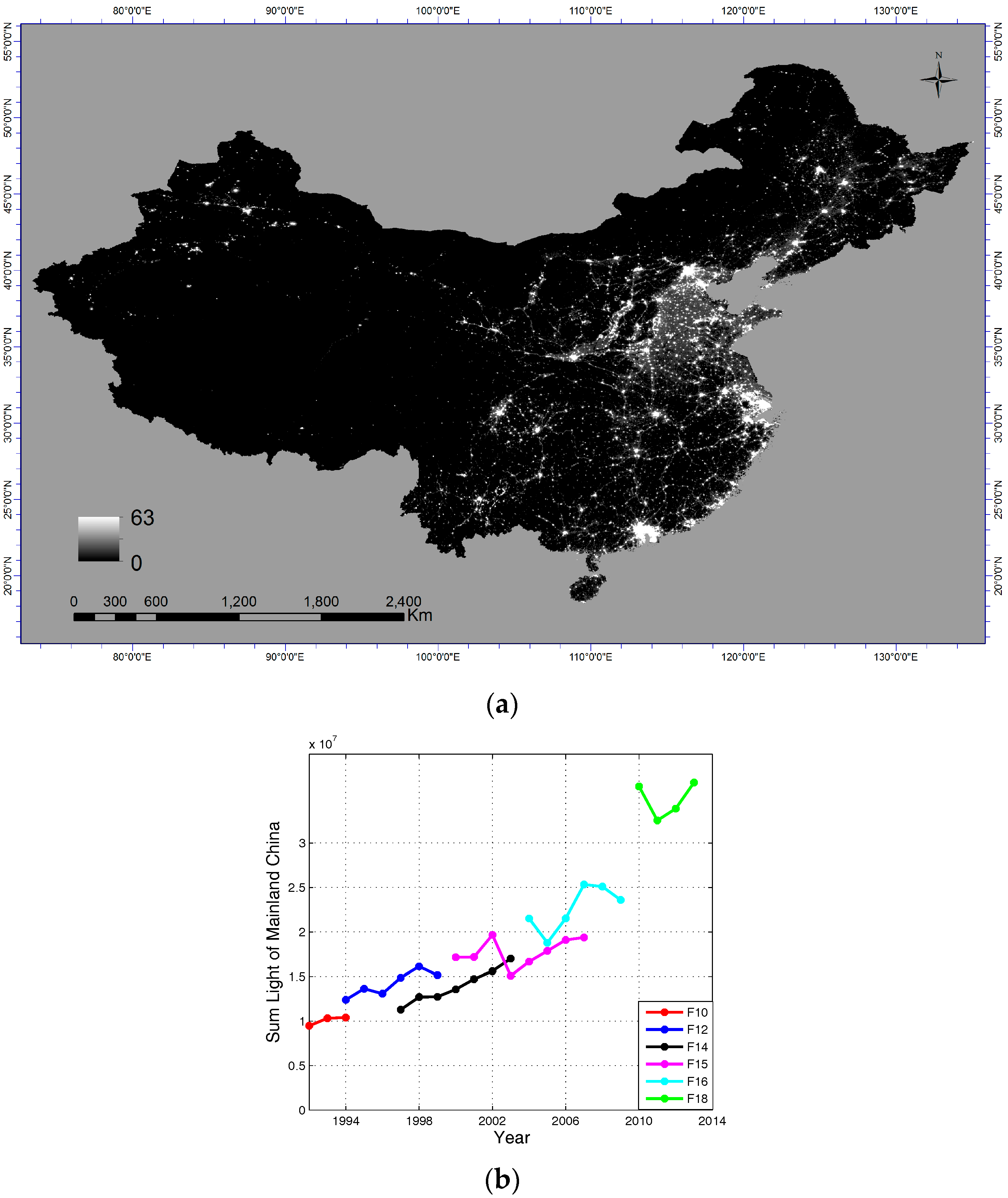
2.1. DMSP/OLS Data Description

DMSP/OLS is used to produce NTL data recording the manmade/natural fires, city lights, and natural gas flaring. It is initially designed to observe the global distribution of clouds and cloud top temperatures, but the use of the OLS’s photo-multiplier tube (PMT) at night gives the OLS a unique capability to gather the low lights data of the earth’s surface. The DMSP/OLS satellites move in a sun-synchronous low altitude polar orbit with a swath width of 3000 km, and they have the capability of collecting a complete set of NTL data with a global coverage twice a day [41]. NTL data have a spatial resolution of 1 km at the equator and 0.8 km at 40°N, and they can be freely downloaded since 1992 for each year. In fact, the data for each year are a global annual cloud-free composite of DMSP/OLS visible band imageries captured on the individual orbits of one satellite. Apart from the minimum influences of atmospheric effects, the data were screened by automatic algorithms to improve the quality by excluding the detections from sunlit, glare, moonlit, and clouds [41,42]. For this study, we downloaded the annual stable lights products from 1992 to 2013, as shown in Figure 1a for the data of Mainland China in 2002. It should be noted that the impacts from fires, ephemeral lights and background noise were also removed from the NTL data by employing detection techniques [15].
However, the time series of NTL data cannot be directly used to examine the growth patterns. This might be attributed to two reasons. Firstly, NTL data were collected by different satellites, and the OLS sensors do not have on-board calibration [43]. Secondly, NTL data collected by different satellites in the same year had no strict inter-calibration [24,43]. Without on-board calibration and inter-calibration, NTL data might contain a significant number of unstable lit-pixels, which could cause large discrepancies in DN values between two satellites for the same year and abnormal fluctuations in DN values for the same satellite in different years. As shown in Figure 1b, we plot the summation of DN values over years for different satellites. It can be clearly seen that there is a large discrepancy of DN values in 1994 for two satellites F10 and F12 and that abnormal fluctuations of DN values are observed for satellite F15 between 2002 and 2003. Hence, it is requisite to preprocess the time series of NTL data to rectify the unstable lit-pixels, which makes the DN values between different years or among different satellites continuous and comparable.

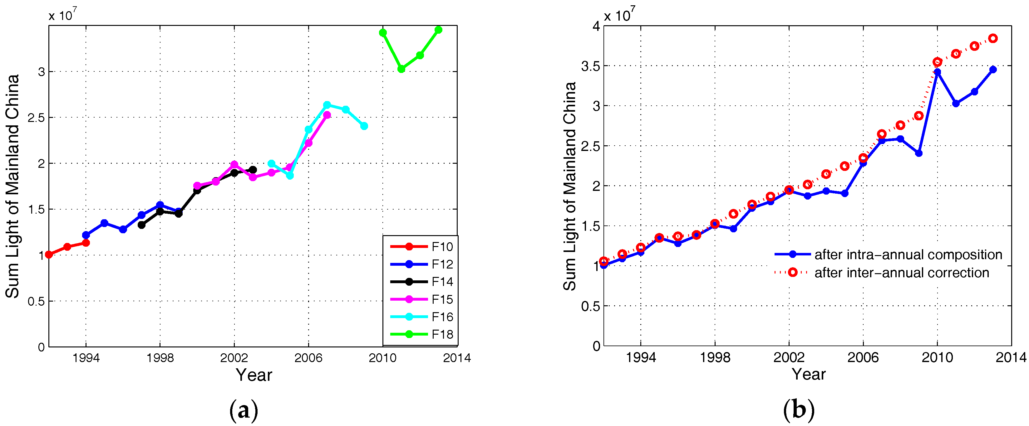
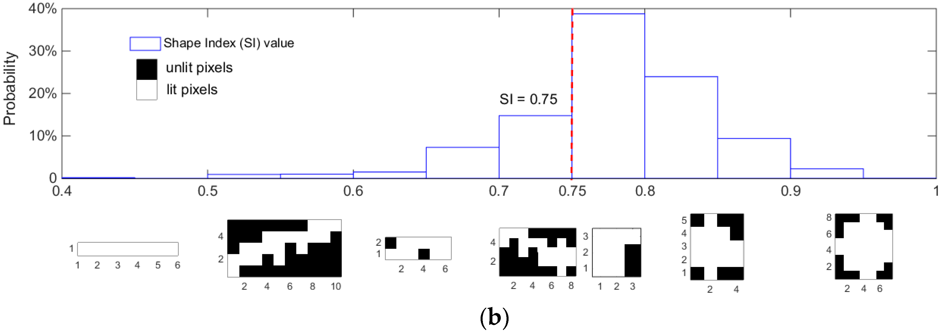
2.2. DMSP/OLS Data Preprocessing

Firstly, we adopt the method proposed by [43] to inter-calibrate the NTL time series data. The essence of this method is to construct a quadratic polynomial regression model to correct the observed DN values. In this study, we constructed the regression model for each NTL image with R-squared value greater than 0.92. After inter-calibration, the quality of NTL time series data is significantly improved in terms of compatibility and continuity. As shown in Figure 2a, the summation of DN values is plotted over years for different satellites, where discrepancies of DN values between two satellites in the same year are diminished and abnormal fluctuations of DN values for the same satellite in different years are reduced. However, small discrepancies are not completed removed, for instance, F10-1994 and F12-1994. Hence, the inter-calibrated NTL time series data should be further preprocessed for the compatibility and consistency of DN values.
Secondly, intra-annual composition and inter-annual correction are conducted sequentially on the time series of NTL data, which aims to further improve the compatibility and consistency of DN values [30]. The objective of intra-annual composition is to make use of the information derived from two satellites for the same year. The calibrated DN values are zero if the pixels are detected by only one satellite, and they are otherwise assigned by the average values of two NTL imageries. The purpose of inter-annual correction is to ensure the DN values of NTL data are not decreasing from 1992 to 2013 and to reflect the actual growth situations of metropolitans in Mainland China. This calibration is based on the assumption that DN extent in metropolitan is expanding and DN values are becoming much brighter (Please refer to [30] for detailed technique). After intra-annual composition and intra-annual correction, as shown in Figure 2b, we find that the total DN values of NTL data is gradually increased from 1992 to 2013 and that a significant increase occurred from 2009 to 2010.

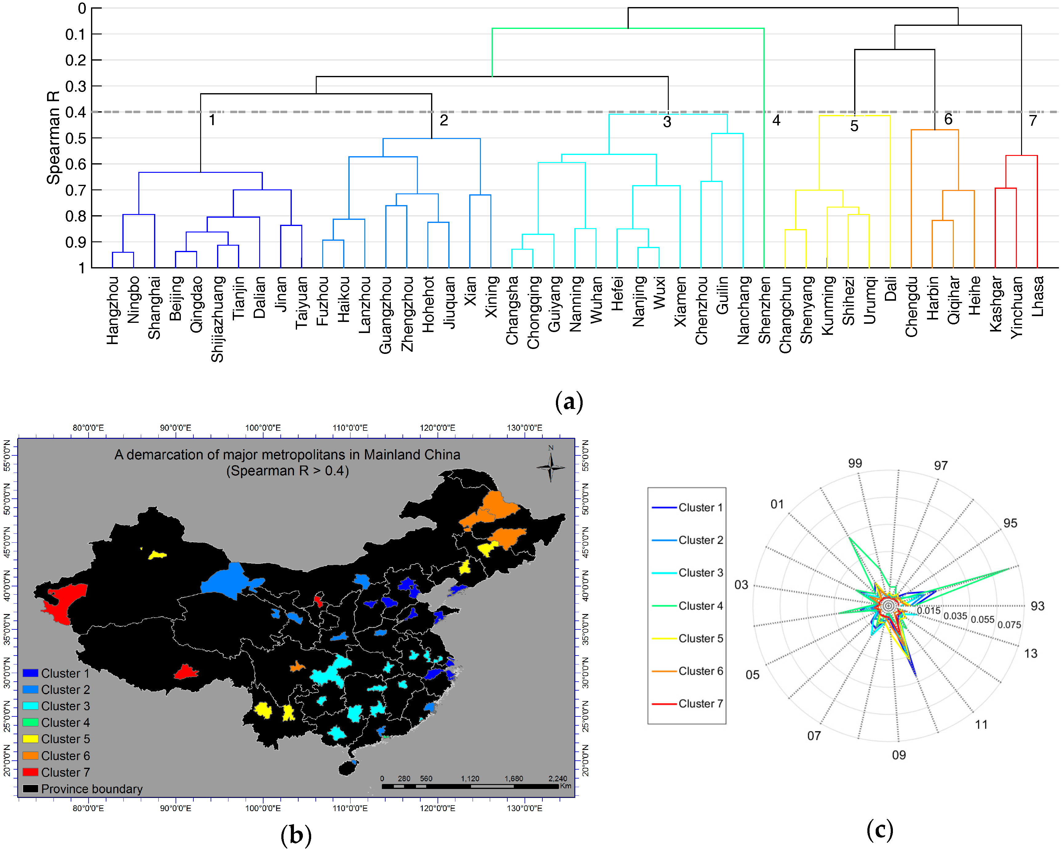
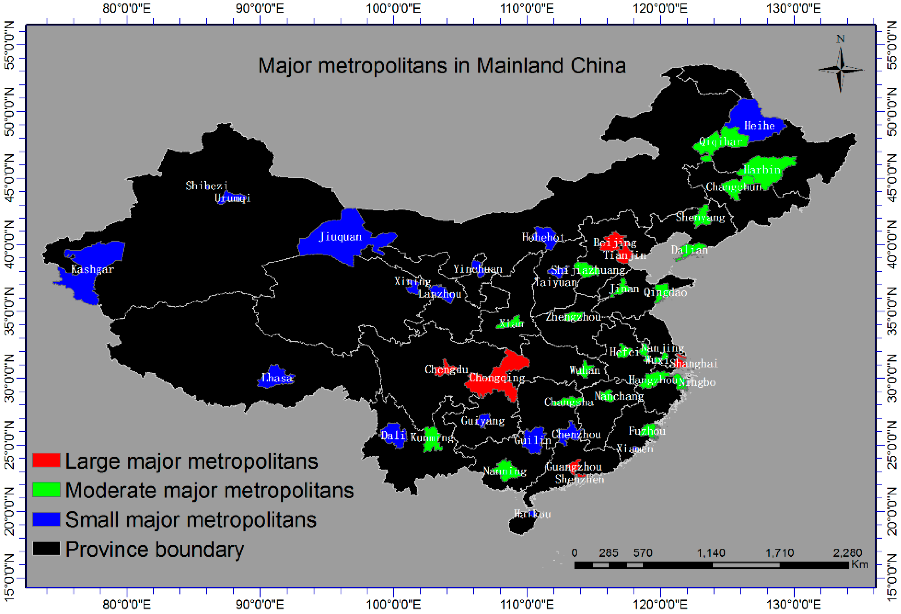
2.3. Selecting Major Metropolitans in Mainland China

Metropolitans in Mainland China have the same boundaries as the administrative divisions, which typically include central cities and the surrounding counties or towns [39]. In this study, a total number of 45 major metropolitans were selected owing to the availability of socioeconomic data. Basically, the metropolitans should be selected with a good spatial coverage. As shown in Figure 3, according to the population in 2013, we selected 7 cities (with population greater than 10 million) as large major metropolitans, 21 cities (with population greater than 5 million but less than 10 million) as moderate major metropolitans, 17 cities (with population less than 5 million) as small major metropolitans. As shown in Figure 3, the selected metropolitans are in general evenly distributed in Mainland China. Besides, simple statistic information suggests that the selected metropolitans take a proportion of 21.6% in population and have a percentage of 44.4% in Gross Domestic Product (GDP) in 2013.

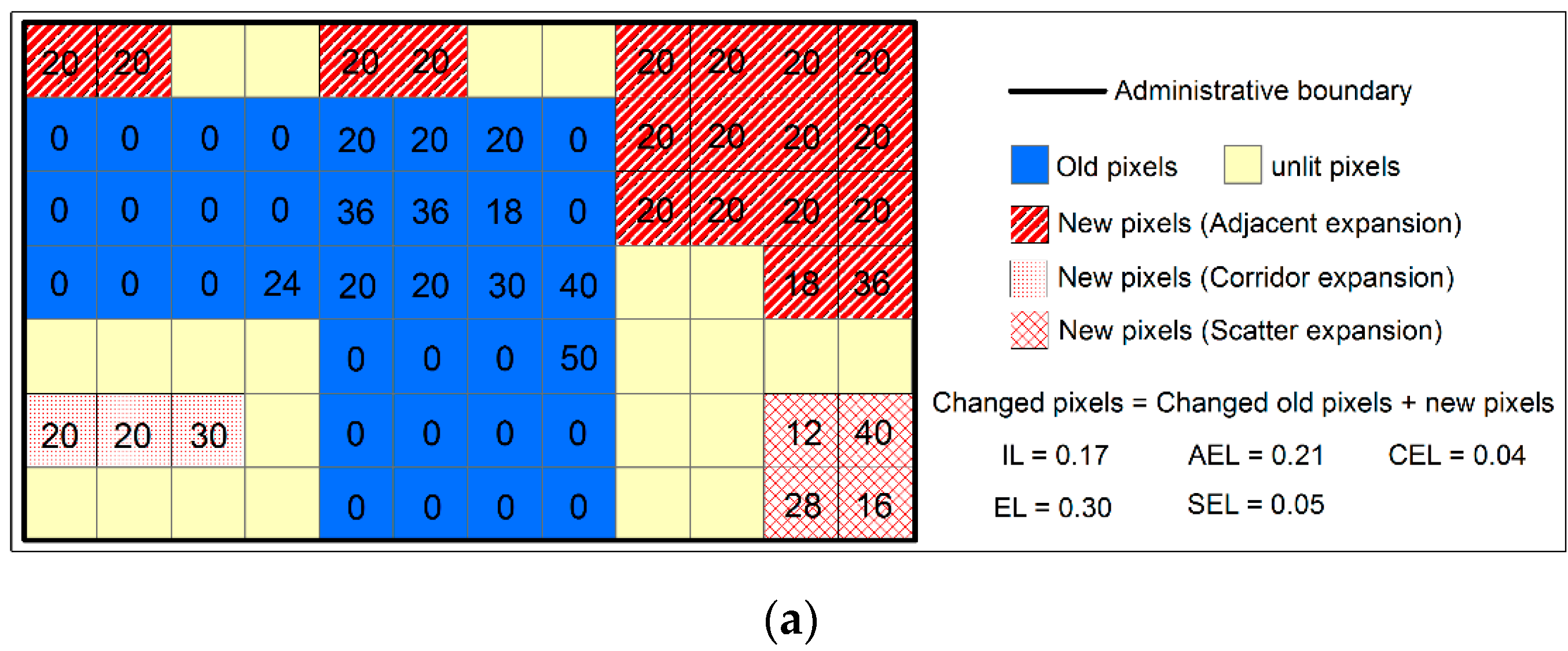
2.4. Measuring Metropolitan Growth with Intensification and Expansion

It is our assumption that the growth of metropolitan might resemble the evolution of street network [44] or airport network [45], which hints that the growth can be modelled as a gradual progress mixed with intensification and expansion. In reality, intensification can be seen as the dynamics of housing units, roads, or even land use changes, which is related to human activities in terms of demographic dynamics or economic development, and expansion can be observed as low density development at urban fringe, which is also related to human activities by consuming unexploited land and displays different spatial types. Hence, intensification and expansion in metropolitan can be examined using the change of lit-pixels, because it has already been confirmed that DN values are highly correlated with population or other socioeconomic factors.
To quantitatively measure the intensification, we propose intensification level (IL), which can be calculated as the change of DN values normalized by metropolitan area as shown in Equation (1).
I L ( t ) = i C P ( t ) Δ D N i N C P ( t ) × D N m a x × A r e a C P ( t ) A r e a M e t r o p o l i t a n
where in the year t, IL(t) is the intensification level, CP(t) is the set of changed pixels, Δ DNi is the changed DN value of the ith pixels, NCP(t) is the number of changed pixels, DNmax is the saturated DN value of 63, AreaCP(t) is the area of changed pixels, and AreaMetropolitan is the area of metropolitan. In this respect, we can see that information contained in IL is more related to the actual change of the brightness in two consecutive years by filtering out the brightness of DN values contaminated by the same source (such as the atmospheric scattering) to a certain degree. As shown in Figure 4a, an illustration is given to depict the concept of changed pixels and its application on calculating the IL.
To quantitatively measure the expansion, we firstly define new pixels as the ones lit in the current year but not in the previous year and old pixels as the ones lit in two consecutive years (c.f. Figure 4a). Secondly, we propose the concept of expansion level (EL). EL is defined as the change of DN extent normalized by metropolitan area as shown in Equation (2).
E L ( t ) = A r e a N P ( t ) A r e a M e t r o p o l i t a n
where in the year t, EL(t) is the expansion level, NP(t) is the set of new pixels, and AreaNP(t) is the extent of new pixels. Thirdly, expansion in metropolitan is examined by using spatial aggregation method on new pixels to identify three spatial types, namely adjacent, scatter, and corridor expansion (c.f. Figure 4a). Adjacent expansion can be detected as the agglomeration of new pixels that are spatially adjacent to at least one old pixel; scatter expansion can be identified as the agglomeration of new pixels that are isolated from any old pixels and has a relative large value of shape index (SI); corridor expansion is similar to the definition of scatter expansion except that it has a relative small value of SI. In this study, the shape index (SI) of the agglomeration is defined as Equation (3).
S I = A P × P × 4 × P i
where A is the area and P is the total perimeter. Ideally, SI value ranges from 0 to 1, where it has a large value for a circle-like shape and a small value for a belt-like shape. As shown in Figure 4b, we select the optimal SI as 0.75 to distinguish scatter expansion from corridor expansion by checking the shapes of all possible agglomerations. Fourthly, similar to the definition of expansion level, we define the adjacent expansion level (AEL), scatter expansion level (SEL), and corridor expansion level (CEL) as the following Equation (4).
A E L ( t ) = A r e a N P ( t ) A d j a c e n t A r e a M e t r o p o l i t a n ; S E L ( t ) = A r e a N P ( t ) S c a t t e r A r e a M e t r o p o l i t a n ; C E L ( t ) = A r e a N P ( t ) C o r r i d o r A r e a M e t r o p o l i t a n

3. Results

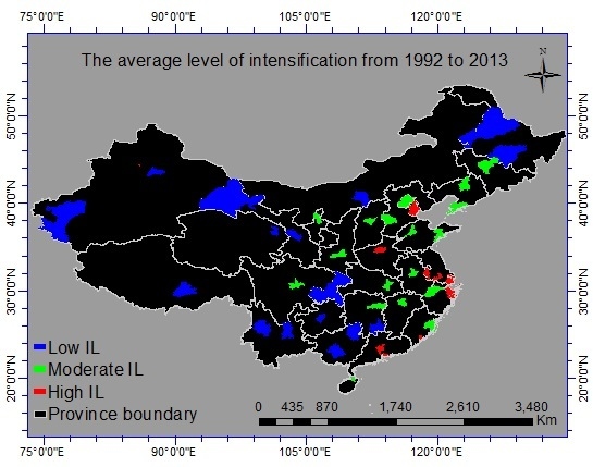
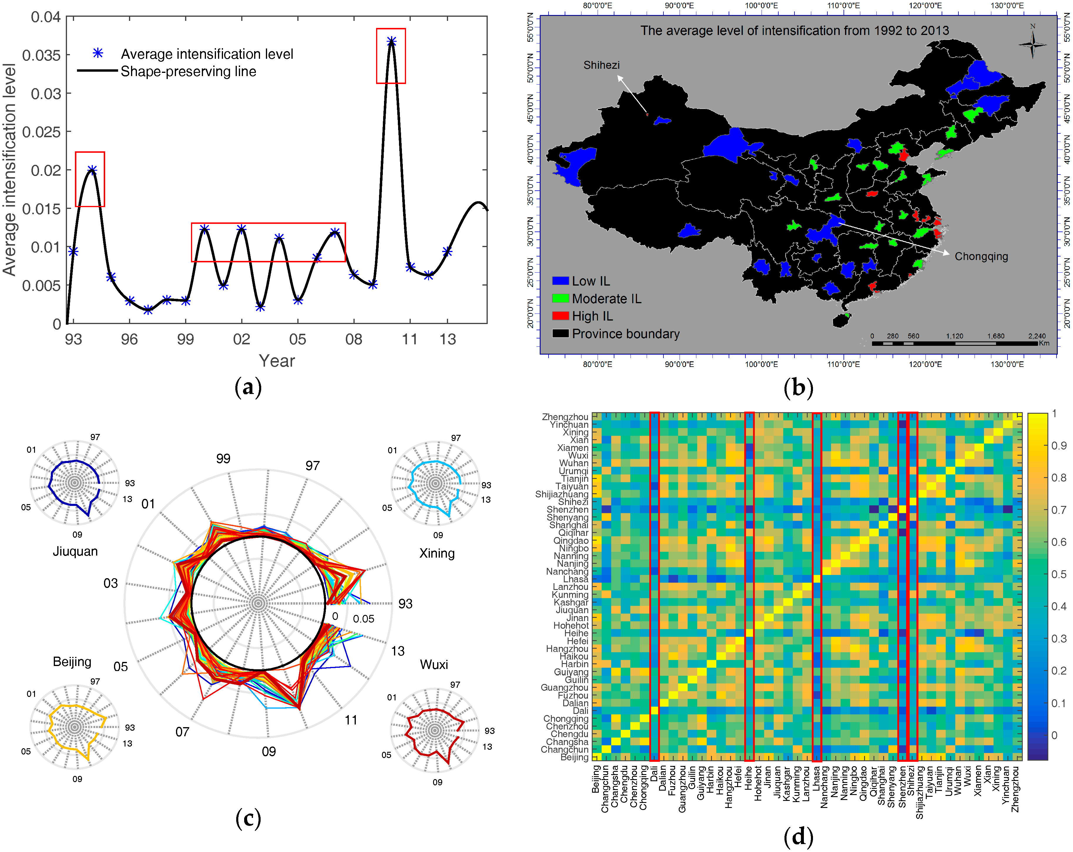
3.1. Growth Patterns from Intensification

We calculate the values of IL for individual metropolitans in each year. Aggregately, annual IL seems to display a cyclical pattern in the two decades (c.f. Figure 5a). Using variance ratio test at the significant level of 5% [46], we confirm that the cyclical pattern is subject to the underlying deterministic process instead of a stochastic process due to the remaining spurious variability in the time series of NTL data. More specifically, it can be roughly divided into a weak rhythm from 1993 to 1999 with a peak in 1994 and a strong rhythm from 2000 to 2013 with a peak in 2010, which coincides well with the stable development period under the reform and opening up policy (such as the approval of specific economic zones for some coastal cities in 1994) and the rapid development period under the coordinated development policy (such as the Western Region Development Plan in 2000) respectively. In addition, as shown in Figure 5b, we display the spatial distribution of the average value of IL for each metropolitan from 1992 to 2013. The map gives two interesting findings. Firstly, it indicates that IL in large metropolitans are on average 48.4% higher than moderate metropolitans and 133.9% higher than small metropolitans. Secondly, Chongqing, as a large metropolitan, displays a low level of intensification, and Shihezi, as a small metropolitan, shows a high level of intensification. This counter-intuitive finding suggests the effect of geographic constraint on the metropolitan intensification. For instance, Chongqing, known as the mountain city, has around 76% of mountain area in its administrative boundary; Shihezi is a small and flattened area located in the north of Tianshan Mountain and in the south of Gulbentonggut desert.
To display the characteristics of individual metropolitans, we use polar plot where IL is plotted in temporal counter-clockwise direction with value increasing from the centre to circumference. Two findings can be reported. Firstly, metropolitans seem to display evolution pattern with variations in each year. Specifically, the maximum variations occurred in 1994 and 2010 respectively, where the coast large metropolitans including Shenzhen and Shanghai experienced the most in 1994 and the inland moderate metropolitans including Wuxi and Ningbo experienced the most in 2010. Secondly, metropolitans seem to show evolution pattern with similar trend over the years. The similar pattern is further verified by a quantitative spearman correlation analysis on each pair of metropolitans. As shown in Figure 5d, 99% of pairs are positively correlated with each other and 73% of them have the spearman correlation coefficient values larger than 0.4. It reveals the macro universal pattern of the evolution of intensification among metropolitans guided by the implementations of the top-down based institutional forces, although five metropolitans including Dali, Heihe, Lhasa, Shiheze, and Shenzhen show weak correlations with others (say the average correlation values are less than 0.4), which puts forward an open question.
The evolution with similar trend in intensification further points out a clustering of metropolitans. It means that some metropolitans are more likely to be clustered together with high correlation values, while others may be separated from each other due to poor correlation. For instance, Hangzhou and Ningbo are related with correlation coefficient value as high as 0.94. To obtain the clusters, we use the bottom-up based hierarchical clustering method, which group metropolitans based on the spearman correlation coefficients. More specifically, each metropolitan starts in its own cluster, and pairs of clusters are merged as one moves up the hierarchy in a greedy manner, and eventually a Dendrogram is constructed when all the metropolitans are merged as one cluster. As shown in Figure 6a, clusters in different scales could be derived using different correlation coefficient threshold values. For the purpose of illustration, we use threshold value as 0.4 to obtain 7 clusters. As show in Figure 6b, we find that metropolitans with the similar evolution of intensification tend to be spatially clustered together, and these clusters suggest new spatial pattern from the aspect of individual metropolitans. For instance, the first cluster includes metropolitans (such as Beijing, Tianjin, Dalian, Jinan, Qingdao, Shijiazhuang, and Taiyuan) in the Bohai Economic Rim and metropolitans (Such as Shanghai, Hangzhou, and Ningbo) in the Yangtze River Delta. However, Shenzhen shows a dissimilar evolution pattern compared with other metropolitans and forms the fourth cluster of itself, which can be mainly attributed to the specific economic zone policy issued as early as in 1980.
Using the polar plot, we present the change of IL with time for each cluster. As shown in Figure 6c, we can observe that the fourth cluster (Shenzhen) experienced the highest level of intensification with an average value of 0.015 and the seventh cluster (Kashgar, Lhasa, and Yinchuan) presented the lowest level of intensification with 0.003. In addition, we report that the evolution patterns at the cluster level are similar to both the aggregated one (Figure 5a) and the individual one (Figure 5c).

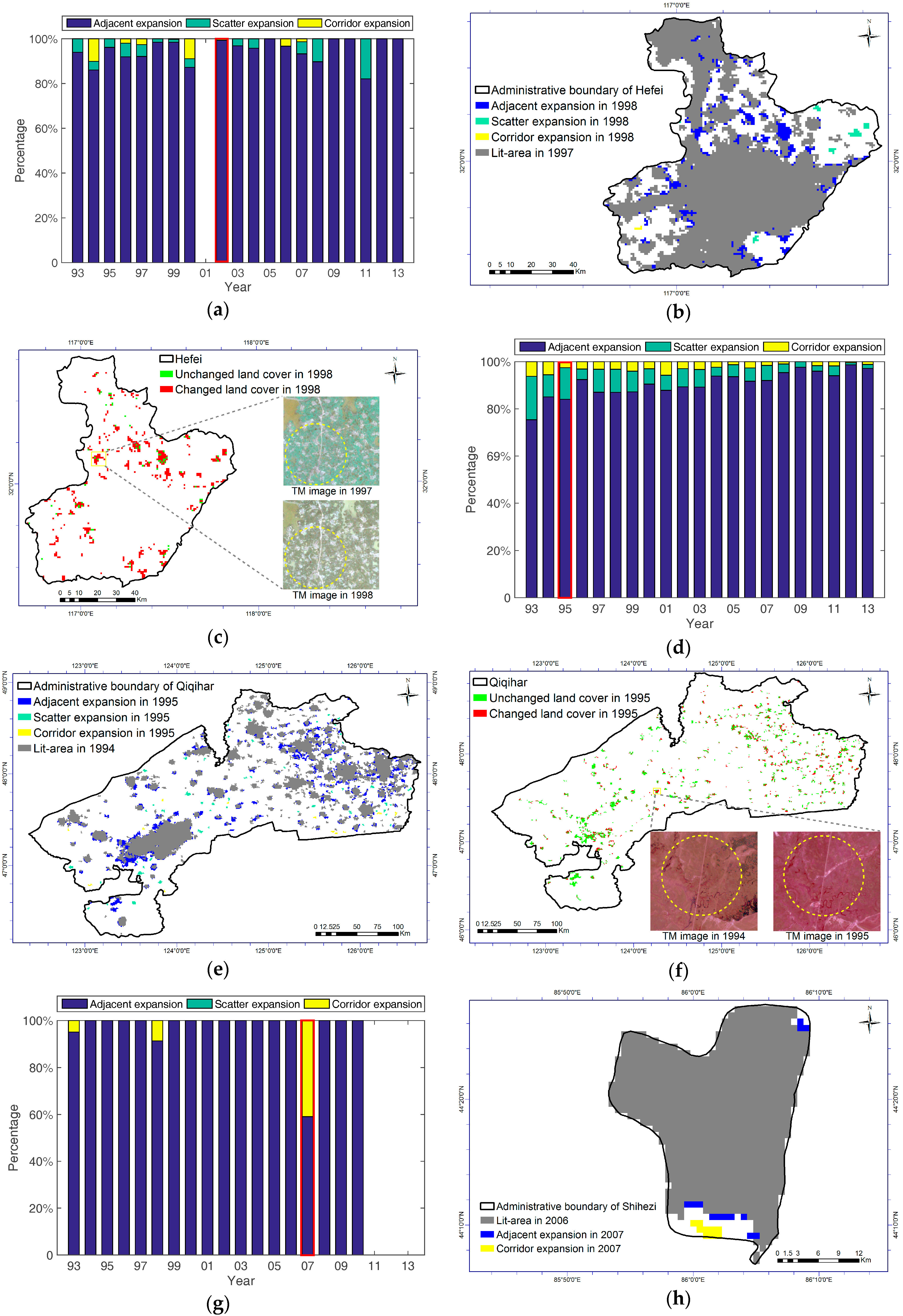
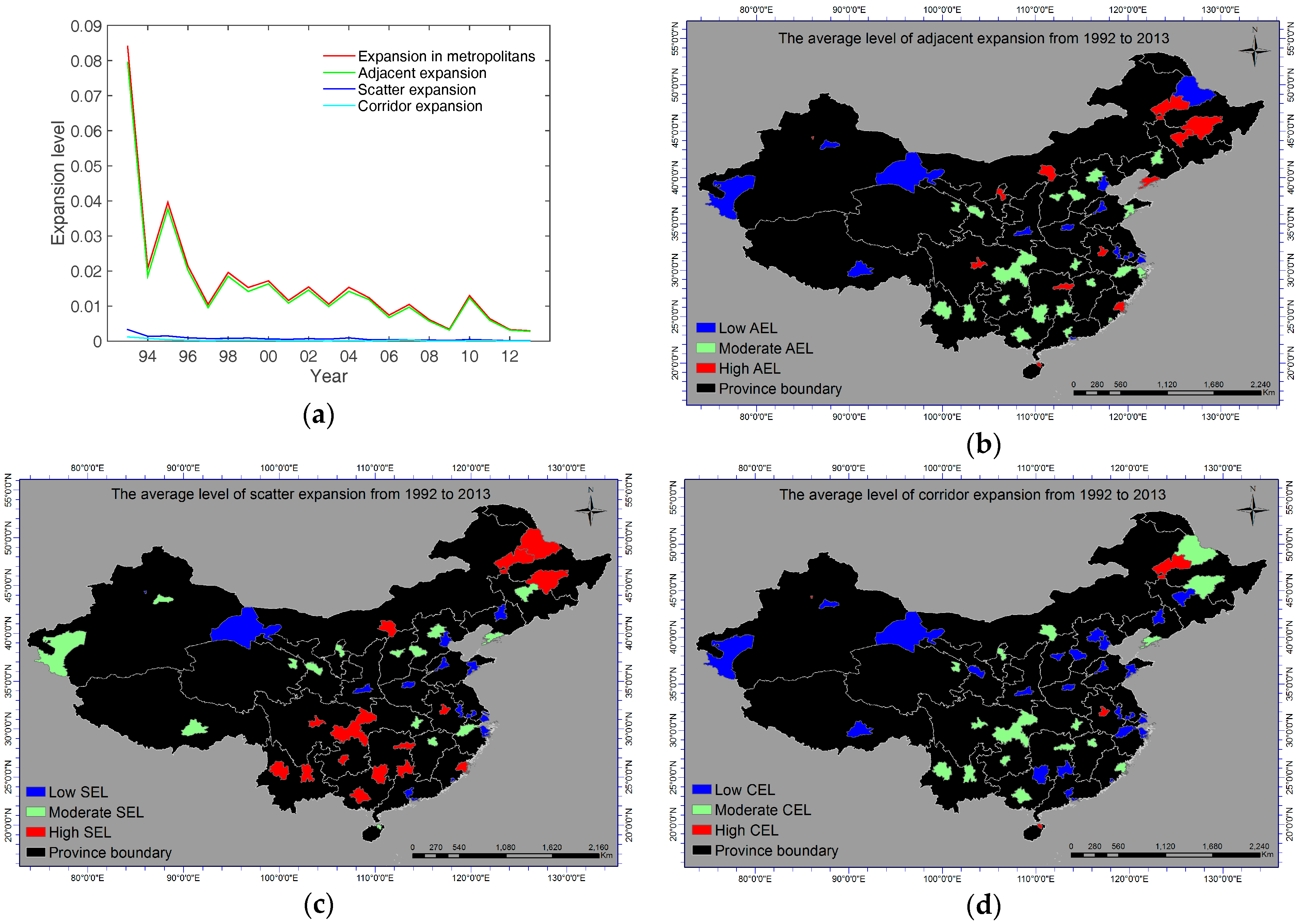
3.2. Growth Patterns from Expansion

Apart from the analysis on the intensification, the growth patterns can be also understood from the expansion or particularly the change of DN extent in the metropolitans. By applying our method to the new pixels of individual metropolitans, we could identify three types of expansion in terms of adjacent, scatter, and corridor. Aggregately, we report that annual EL displays a decreasing trend over time (c.f. Figure 7a), which is different from the cyclical pattern of annual IL shown in Figure 5a. We find that EL in moderate metropolitans seem to be on average 71.2% higher than large metropolitans and 21.0% higher than small metropolitans. In addition, we present the spatial distribution of the average values of AEL (c.f. Figure 7b), SEL (c.f. Figure 7c) and CEL (c.f. Figure 7d) for individual metropolitans, which indicates that inland moderate and small metropolitans are much more likely to display high level of expansion than coast large metropolitans. Statistically, the results suggest that (1) AEL in moderate metropolitans seem to be on average 73.1% higher than large metropolitans and 24.1% higher than small metropolitans; and that (2) SEL (CEL) in small metropolitans seem to be on average 28.6% higher than (equal to) moderate metropolitans and 80.0% (200%) higher than large metropolitans. Hence, we infer that moderate metropolitans are more likely to expand adjacently and small metropolitans are relatively more fragmented in terms of scatter or corridor expansion.
Individually, we argue that the expansion of each metropolitan should be represented by a mixture of three spatial types evolving with time. For the ease of illustration, three metropolitans are selected with large values of AEL, SEL, and CEL. Firstly, Hefei is selected as a representative of adjacent expansion. As shown in Figure 8a, it displayed pure contiguous expansion in 11 years, and map in Figure 8b visualized where adjacent expansion occurred in 1998, and map in Figure 8c displayed the actual spatial changes of land cover in Landsat TM images with an overall accuracy (OA) of 86.9%. Secondly, Qiqihar is selected as a representative of scatter expansion. As shown in Figure 8d, it displayed scatter expansion from 1993 to 2013 although its proportion was in a decreasing trend, and map in Figure 8e illustrated the intensely distributed scatter expansion with malachite green color in 1995, and map in Figure 8f displayed the actual spatial changes of land cover in Landsat TM images with an OA of 78.4%. Thirdly, Shihezi is selected as a representative of corridor expansion. As shown in Figure 8g, we can see that it only experienced adjacent and corridor expansion in the two decades and a corridor expansion occurred in 2007. Map in Figure 8h depicted a clear belt-shaped corridor expansion near the south of its administrative boundary with yellow color, and map in Figure 8i displayed the actual spatial changes of land cover in Landsat TM images with an OA of 56.3%. Therefore, these results can be useful for the policy making or planning under sustainable urban development.

3.3. Relationship between Intensification and Expansion for Each Metropolitan

Until now we have elaborated the growth patterns from the aspects of intensification and expansion, this section intends to understand how intensification is related to expansion for each metropolitan. To answer this question, we take a look at the relationship between IL and EL over time for individual metropolitans, because each metropolitan might reveal a distinct relationship. As shown in Table 1, two facts could be obtained. First, remarkable linear relationships can be observed for small metropolitans, such as Lhasa and Kashgar, but they have different slope values indicating the different velocities of expansion given per unit increase of intensification. Specifically, it is reported that Heihe is the metropolitan with the fastest speed of expansion owing to the largest slope value. Second, there are no clear relationships for large or moderate metropolitans as the slope values are fluctuated around zero, which indicates that the change of DN values in intensification has nothing to do with the change of DN extent in expansion.

4. Discussion and Limitations

4.1. On Growth Patterns in Terms of Intensification and Expansion

Our study borrows the idea from the evolution of networks [44,45], which regards growth in metropolitan as a gradual progress mixed with intensification and expansion in terms of DN change. This makes our work different from other studies in the literature from three aspects: (1) growth patterns were examined at the metropolitan level instead of at the urban level [27,47]; (2) growth patterns were examined by employing all lit-pixels instead of the urban-pixels [4,32,38]; (3) growth patterns were modeled by integrating intensification and expansion together instead of concentrating on either urban expansion [30,31,47] or urbanization [25,28].
Aggregately, our results suggest that annual IL displays a cyclical trend and annual EL shows a decreasing trend. Large metropolitans tend to have a higher level of intensification than moderate or small metropolitans, while moderate or small metropolitans tend to have a higher level of expansion than large ones. Specifically, by decomposing the expansion into adjacent, scatter, and corridor expansion, we report that moderate metropolitans are likely to experience high level of adjacent expansion and small metropolitans are likely to appear as scatter or corridor expansion.
Individually, our results reveal that metropolitans with the similar evolution of intensification tend to be spatial clustered together. This finding not only can be used to confirm the intensification patterns, but also provides a new spatial division to be compared with government specified urban economic rims. Our results further elaborate that metropolitans display different evolution of expansion with a mixture of three spatial types. Given a metropolitan, we can give the policy makers or urban planners the information on how much and where the three types of expansion occurred in the current year.
In addition, we take a look at the relationship between intensification and expansion. Our results indicate that intensification in metropolitan is not necessarily related to its expansion. Specifically, small metropolitans tend to have remarkable linear relationships between their IL and EL, and large or moderate metropolitans have no relationship at all. These findings suggest that large or moderate metropolitans have already been aware of the negative effects from expansion and they might have made policies to curb it. However, small metropolitans are still undergoing a high speed of expansion due to intensification, and hence, more attention should be paid to them.

4.2. On Socio-Economic Correlation with IL and EL in Each Year

It has been reported widely in the literature that DN values were highly correlated to many socio-economic indicators [19,22,28,48,49]. As the measurements on growth patterns, it is interesting to examine whether IL and EL are related to socio-economic indicator such as Gross Domestic Product (GDP) or population (POP). By doing so, we can also verify the feasibility of employing IL and EL on measuring growth in metropolitans. To keep the consistency, we compute the change of GDP or POP per unit area in two consecutive years, which is denoted as Δ GDP and Δ POP respectively. Our correlation results suggest that IL and EL are highly correlated with Δ GDP but are poorly correlated with Δ POP across metropolitans in each year. As shown in Table 2, we display the linear models of IL and EL with Δ GDP. It can be generally found that IL is positively correlated with Δ GDP and EL is negatively correlated with Δ GDP. On average, we can say that around 49.2% of variability in GDP change per unit area can be explained by IL and EL. Therefore, we argue that IL and EL can be used as reliable measurements to examine the growth patterns, although a thorough understanding on the underlying mechanism needs further investigation.

4.3. Limitations

Three limitations can be found in this study. Firstly, although this study attempts to verify the reliability of our results by using statistical significance test and Landsat TM image, there is still a large room to reduce the impacts of spurious variability in the image time series on the growth patterns. For instance, the usage of advanced preprocessing techniques, such as the empirical orthogonal function analysis [15] and the sampling strategy by identifying pseudoinvariant features [50], will be our future work.
Secondly, the quick saturation problem of DMSP/OLS sensors is a potential limitation on using IL. For instance, an increase in radiance for a saturated pixel would not be detected if its DN value was already 63 in the previous year. To quantitatively understand this limitation, we compute the average percentages of saturated pixels (DN value = 63) and unsaturated pixels (DN value < 63) from 1993 to 2013 for individual metropolitans respectively. As shown in Figure 9, three facts can be observed: (1) All major metropolitans have a larger percentage of unsaturated pixels than saturated pixels; (2) For each metropolitan on average, 98% of lit-pixels are unsaturated, and only 2% of them are saturated; (3) The top three metropolitans with the largest percentages of saturated pixels are Shenzhen with 24%; Shanghai with 19%; and Beijing with 8%. Hence, the results on the growth patterns of Shenzhen and Shanghai require further investigation, but the results on all other metropolitans should be reliable due to the negligible influence of quick saturation problem on growth patterns. This is another major reason why we examine growth patterns using lit-pixels.
Thirdly, the DMSP/OLS NTL data have a relative coarse spatial resolution, which could constrain their application on small scale of metropolitan studies. Therefore, our attention will be paid to examine the socio-economic activities within metropolitans or regions using the data with fine resolution from new sensors, such as the imageries obtained from the Visible Infrared Imaging Radiometer Suite (VIIRS) and the National Polar-orbiting Operational Environmental Satellite System (NPOESS).

5. Conclusions

Using DMSP/OLS data, this study contributes to the literature with a new perspective to examine growth patterns at the metropolitan level by integrating intensification and expansion together. We propose IL and EL to examine the intensification and expansion in metropolitans over two decades. In this respect, we select 45 major metropolitans in Mainland China, and their growth patterns are reported.
The results suggest that aggregately annual IL displayed a cyclical pattern with two peaks in 1994 and 2010 respectively, while annual EL exhibited a fluctuated decreasing trend over time. Large metropolitans tended to have a higher level of intensification than moderate or small metropolitans, while moderate or small metropolitans tended to have a higher level of expansion than large ones. Particularly, moderate metropolitans were likely to experience adjacent expansion, and small metropolitans were likely to encounter fragmented development in terms of scatter or corridor expansion. Individually, our results show that metropolitans with the similar evolution of intensification over time were probably to be spatially adjacent to each other, and these clusters provide a new spatial division to be compared with the government specified urban economic rims, such as the Bohai Economic Rim or the Yangtze River Delta. Besides, we vividly present the evolution of expansion for three selected metropolitans, which could answer where and how much the expansion occurred in each year. Particularly, the spatial expansion is validated by a comparison with the land cover changes in Landsat TM images, and the results show an overall accuracy of 86.9%, 78.4%, and 56.3% with respect to the three metropolitans.
Lastly, the results reveal remarkable linear relationships between IL and EL over time for small metropolitans but poor relationship for large or moderate ones. Importantly, we conclude that IL and EL can be used as reliable measurements to examine the growth patterns in metropolitans owing to their high correlation with the change of GDP per unit area in each year. We believe that the results reported can be used for a better planning and policy making in sustainable development.

Acknowledgments

We would like to acknowledge the National Natural Science Foundation of China who supported this work with Award numbers: 41401453 and 41331175. We would also like to thank the financial support from the Doctoral Program of Higher Education of China with Award number 20130141120075. We would also like to extend our gratitude to Yuqian Li for her research assistance.

Author Contributions

T.J. conceived and designed the experiments; T.J. and K.C. performed the experiments; T.J., K.C. and J.W. analyzed the data; J.W. contributed materials; T.J. wrote the paper.

Conflicts of Interest

The authors declare no conflict of interest.

References

  1. United Nations. World Urbanization Prospects: The 2014 Revision; United Nations Population Division: New York, NY, USA, 2014. [Google Scholar]
  2. Frey, W. Will This Be the Decade of Big City Growth? The Brookings Institution: Washington, DC, USA, 2014. [Google Scholar]
  3. Song, X.P.; Sexton, J.O.; Huang, C.; Channan, S.; Townshend, J.R. Characterizing the magnitude, timing and duration of urban growth from time series of Landsat-based estimates of impervious cover. Remote Sens. Environ. 2016, 175, 1–13. [Google Scholar] [CrossRef]
  4. Zhang, Q.; Su, S.L. Determinants of urban expansion and their relative importance: A comparative analysis of 30 major metropolitans in China. Habitat Int. 2016, 58, 89–107. [Google Scholar] [CrossRef]
  5. Yu, B.; Shu, S.; Liu, H.; Song, W.; Wu, J.; Wang, L.; Chen, Z. Object-based spatial cluster analysis of urban landscape pattern using nighttime light satellite images: A case study of China. Int. J. Geogr. Inf. Sci. 2014, 28, 2328–2355. [Google Scholar] [CrossRef]
  6. Marull, J.; Font, C.; Boix, R. Modelling urban networks at mega-regional scale: Are increasingly complex urban systems sustainable? Land Use Policy 2015, 43, 15–27. [Google Scholar] [CrossRef]
  7. Pacione, M. Urban Geography—A Global Perspective; Routledge: London, UK, 2009. [Google Scholar]
  8. Salvati, L.; Venanzoni, G.; Serra, P.; Carlucci, M. Scattered or polycentric? Untangling urban growth in hree southern European metropolitan regions through exploratory spatial data analysis. Ann. Reg. Sci. 2016, 57, 1–29. [Google Scholar] [CrossRef]
  9. Han, L.; Zhou, W.; Li, W.; Li, L. Impact of urbanization level on urban air quality: A case of fine particles (PM2.5) in Chinese cities. Environ. Pollut. 2014, 194, 163–170. [Google Scholar] [CrossRef] [PubMed]
  10. Shi, K.; Chen, Y.; Yu, B.; Xu, T.; Li, L.; Huang, C.; Liu, R.; Chen, Z.; Wu, J. Urban expansion and agricultural land loss in China: A multiscale perspective. Sustainability 2016, 8, 790. [Google Scholar] [CrossRef]
  11. Fverboven, H.; Uyttenbroeck, R.; Brys, R.; Hermy, M. Different responses of bees and hoverflies to land use in an urban-rural gradient show the importance of the nature of the rural land use. Landsc. Urban Plan. 2014, 126, 31–41. [Google Scholar] [CrossRef]
  12. Liu, Y.; Wang, Y.; Peng, J.; Du, Y.; Liu, X.; Li, S.; Zhang, D. Correlations between urbanization and vegetation degradation across the world’s metropolises using DMSP/OLS nighttime light data. Remote Sens. 2015, 7, 2067–2088. [Google Scholar] [CrossRef]
  13. Vramachandra, T.; Haithal, B.; Durgappasanna, D. Insights to urban dynamics through landscape spatial pattern analysis. Int. J. Appl. Earth Obs. Geoinf. 2012, 18, 329–343. [Google Scholar]
  14. Ghosh, T.; Anderson, S.; Elvidge, C.D.; Sutton, P.C. Using nighttime satellite imagery as a proxy measure of human well-being. Sustainability 2013, 5, 4988–5019. [Google Scholar] [CrossRef]
  15. Small, C.; Elvidge, C.D. Night on Earth: Mapping decadal changes of anthropogenic night light in Asia. Int. J. Appl. Earth Obs. Geoinf. 2013, 22, 40–52. [Google Scholar] [CrossRef]
  16. Sutton, P.; Roberts, D.; Elvidge, C.; Baugh, K. Census from Heaven: An estimate of the global human population using night-time satellite imagery. Int. J. Remote Sens. 2001, 22, 3061–3076. [Google Scholar] [CrossRef]
  17. Elvidge, C.D.; Tuttle, B.T.; Sutton, P.C.; Baugh, K.E.; Howard, A.T.; Milesi, C.; Bhaduri, B.L.; Nemani, R. Global distribution and density of constructed impervious surfaces. Sensors 2007, 7, 1962–1979. [Google Scholar] [CrossRef]
  18. Chen, Z.; Yu, B.; Hu, Y.; Huang, C.; Shi, K.; Wu, J. Estimating house vacancy rate in metropolitan areas using NPP-VIIRS nighttime light composite data. IEEE J. Sel. Top. Appl. Earth Obs. Remote Sens. 2015, 8, 2188–2197. [Google Scholar] [CrossRef]
  19. Sutton, P.C.; Costanza, R. Global estimates of market and non-market values derived from nighttime satellite imagery, land cover, and ecosystem service valuation. Ecol. Econ. 2002, 41, 509–527. [Google Scholar] [CrossRef]
  20. Doll, C.N.H.; Muller, J.-P.; Morley, J.G. Mapping regional economic activity from night-time light satellite imagery. Ecol. Econ. 2006, 57, 75–92. [Google Scholar] [CrossRef]
  21. Ghosh, T.; Powell, R.L.; Anderson, S.; Sutton, P.C.; Elvidge, C.D. Informal economy and remittance estimates of India using nighttime imagery. Int. J. Ecol. Econ. Stat. 2010, 17, 16–50. [Google Scholar]
  22. Forbes, D.J. Multi-scale analysis of the relationship between economic statistics and DMSP-OLS night light images. GISci. Remote Sens. 2013, 50, 483–499. [Google Scholar]
  23. Shi, K.; Yu, B.; Huang, Y.; Hu, Y.; Yin, B.; Chen, Z.; Chen, L.; Wu, J. Evaluating the ability of NPP-VIIRS nighttime light data to estimate the gross domestic product and the electric power consumption of China at multiple scales: A comparison with DMSP-OLS data. Remote Sens. 2014, 6, 1705–1724. [Google Scholar] [CrossRef]
  24. Zhang, Q.; Seto, K.C. Mapping urbanization dynamics at regional and global scales using multi-temporal DMSP/OLS nighttime light data. Remote Sens. Environ. 2011, 115, 2320–2329. [Google Scholar] [CrossRef]
  25. Ma, T.; Zhou, C.; Pei, T.; Haynie, S.; Fan, J. Quantitative estimation of urbanization dynamics using time series of DMSP/OLS nighttime light data: A comparative case study from China’s cities. Remote Sens. Environ. 2012, 124, 99–107. [Google Scholar] [CrossRef]
  26. Xu, T.; Ma, T.; Zhou, C.; Zhou, Y. Characterizing spatio-temporal dynamics of urbanization in China using time series of DMSP/OLS night light data. Remote Sens. 2014, 6, 7708–7731. [Google Scholar] [CrossRef]
  27. Gao, B.; Huang, Q.; He, C.; Ma, Q. Dynamics of urbanization levels in China from 1992 to 2012: Perspective from DMSP/OLS nighttime light data. Remote Sens. 2015, 7, 1721–1735. [Google Scholar] [CrossRef]
  28. Ma, T.; Yin, Z.; Li, B.; Zhou, C.; Haynie, S. Quantitative estimation of the velocity of urbanization in China using nighttime luminosity data. Remote Sens. 2016, 8, 94. [Google Scholar] [CrossRef]
  29. Seto, K.C.; Fragkias, M.; Güneralp, B.; Reilly, M.K. A meta-analysis of global urban land expansion. PLoS ONE 2011, 6, e23777. [Google Scholar] [CrossRef] [PubMed]
  30. Liu, Z.; He, C.; Zhang, Q.; Huang, Q.; Yang, Y. Extracting the dynamics of urban expansion in China using DMSP-OLS nighttime light data from 1992 to 2008. Landsc. Urban Plan. 2012, 106, 62–72. [Google Scholar] [CrossRef]
  31. Gao, B.; Huang, Q.; He, C.; Sun, Z.; Zhang, D. How does sprawl differ across cities in China? A multi-scale investigation using nighttime light and census data. Landsc. Urban Plan. 2016, 148, 89–98. [Google Scholar] [CrossRef]
  32. Wei, Y.; Liu, H.; Song, W.; Yu, B.; Xiu, C. Normalization of time series DMSP-OLS nighttime light images for urban growth analysis with Pseudo Invariant Features. Landsc. Urban Plan. 2014, 128, 1–13. [Google Scholar] [CrossRef]
  33. Peter, C.; Nicola, P.; Didier, S. Dynamics and spatial distribution of global nighttime lights. EPJ Data Sci. 2014, 3, 1–26. [Google Scholar]
  34. Wu, W.; Zhao, S.; Zhu, C.; Jiang, J. A comparative study of urban expansion in Beijing, Tianjin and Shijiazhuang over the past three decades. Landsc. Urban Plan. 2015, 134, 93–106. [Google Scholar] [CrossRef]
  35. You, H. Quantifying megacity growth in response to economic transition: A case of Shanghai, China. Habitat Int. 2016, 53, 115–122. [Google Scholar] [CrossRef]
  36. Haas, J.; Ban, Y. Urban growth and environmental impacts in Jing-Jin-Ji, the Yangtze River Delta and the Pearl River Delta. Int. J. Appl. Earth Obs. Geoinf. 2014, 30, 42–55. [Google Scholar] [CrossRef]
  37. Ma, Q.; He, C.; Wu, J.; Liu, Z.; Zhang, Q.; Sun, Z. Quantifying spatiotemporal patterns of urban impervious surfaces in China: An improved assessment using nighttime light data. Landsc. Urban Plan. 2014, 130, 36–49. [Google Scholar] [CrossRef]
  38. Liu, Z.; He, C.; Wu, J. General spatiotemporal patterns of urbanization: An examination of 16 World Cities. Sustainability 2016, 8, 41. [Google Scholar] [CrossRef]
  39. Vogel, R.K.; Savitch, H.V.; Xu, J.; Yeh, A.G.O.; Wu, W.; Sancton, A.; Kantor, P.; Newman, P.; Tsukamoto, T.; Cheung, P.T.Y.; et al. Governing global city regions in China and the West. Prog. Plan. 2010, 73, 1–75. [Google Scholar] [CrossRef]
  40. Chen, M.; Liu, W.; Lu, D. Challenges and the way forward in China’s new type urbanization. Land Use Policy 2016, 55, 334–339. [Google Scholar] [CrossRef]
  41. Elvidge, C.D.; Baugh, K.E.; Kihn, E.A.; Kroehl, H.W.; Davis, E.R. Mapping city lights with nighttime data from the DMSP operational linescan system. Photogram. Eng. Remote Sens. 1997, 63, 727–734. [Google Scholar]
  42. Baugh, K.E.; Elvidge, C.D.; Ghosh, T.; Ziskin, D. Development of a 2009 stable lights product using DMSP-OLS data. In Proceedings of the 30th Asia-Pacific Advanced Network Meeting, Sydney, Australia, 7–11 February 2010. [Google Scholar]
  43. Elvidge, C.D.; Ziskin, D.; Baugh, K.E.; Tuttle, B.T.; Ghosh, T.; Pack, D.W.; Erwin, E.H.; Zhizhin, M. Fifteen year record of global natural gas flaring derived from satellite data. Energies 2009, 2, 595–622. [Google Scholar] [CrossRef]
  44. Strano, E.; Nicosia, V.; Latora, V.; Porta, S.; Barthelemy, M. Elementary processes governing the evolution of road networks. Sci. Rep. 2012, 2, 1–8. [Google Scholar] [CrossRef] [PubMed]
  45. Jia, T.; Qin, K.; Shan, J. An exploratory analysis on the evolution of the US airport network. Physica A 2014, 413, 266–279. [Google Scholar] [CrossRef]
  46. Lo, A.W.; MacKinlay, A.C. The Size and Power of the Variance Ratio Test. J. Econ. 1989, 40, 203–238. [Google Scholar] [CrossRef]
  47. Pandey, B.; Joshi, P.K.; Seto, K.C. Monitoring urbanization dynamics in India using DMSP/OLS night time lights and SPOT-VGT data. Int. J. Appl. Earth Obs. Geoinf. 2013, 23, 49–61. [Google Scholar] [CrossRef]
  48. Elvidge, C.D.; Baugh, K.E.; Kihn, E.A.; Kroehl, H.W.; Davis, E.R.; Davis, C.W. Relation between satellites observed visible—Near infrared emissions, population, economic activity and electric power consumption. Int. J. Remote Sens. 1997, 18, 1373–1379. [Google Scholar] [CrossRef]
  49. Ebener, S.; Murray, C.; Tandon, A.; Elvidge, C.C. From wealth to health: Modeling the distribution of income per capita at the sub-national level using night-time light imagery. Int. J. Health Geogr. 2005, 4, 5–14. [Google Scholar] [CrossRef] [PubMed]
  50. Zhang, Q.; Pandey, B.; Seto, K.C. A robust method to generate a consistent time series from DMSP/OLS nighttime light data. IEEE Trans. Geosci. Remote Sens. 2016, 54, 5821–5831. [Google Scholar] [CrossRef]
Figure 1. Study area and its DN values: (a) NTL data of Mainland China in 2002 by DMSP/OLS; (b) summation of DN values over years for different satellites before inter-calibration.
Remotesensing 09 00571 g001
Figure 2. Summation of DN values over years for different satellites after preprocessing: (a) inter-calibration; (b) intra-annual composition and inter-annual correction.
Remotesensing 09 00571 g002
Figure 3. Major Metropolitans in Mainland China.
Remotesensing 09 00571 g003
Figure 4. (a) An illustration of measuring intensification and expansion, where 3 agglomerations of adjacent expansion, 1 agglomeration of scatter expansion and 1 agglomeration of corridor expansion are identified; and (b) Probability distribution of SI with respect to different shapes of agglomerations, and a threshold value of 0.75 is determined via a direct visual observation on these dominant shapes.
Remotesensing 09 00571 g004aRemotesensing 09 00571 g004b
Figure 5. Characteristics of intensification: (a) Annual average IL over years; (b) Map of the average IL for each metropolitan from 1992 to 2013; (c) Polar plot of IL with time, where metropolitans are colored from blue to red according to its average value, and cities with the maximum, 30 percentiles, 70 percentiles, and the minimum average value of IL are Wuxi, Beijing, Xining, and Jiuquan respectively; (d) Spearman correlation coefficients of IL for each pair of metropolitans.
Remotesensing 09 00571 g005
Figure 6. Clustering of major metropolitans: (a) Dendrogram of major metropolitans; (b) Map of the 7 clusters; (c) Polar plot of IL over time with respect to the clusters.
Remotesensing 09 00571 g006
Figure 7. Characteristics of expansion: (a) Annual average EL (AEL, SEL, CEL) over years; and Map of the average values of (b) AEL, (c) SEL, (d) CEL for metropolitans.
Remotesensing 09 00571 g007
Figure 8. Mixed expansion patterns and accuracy assessments for selected metropolitans: (a) Hefei from 1993 to 2013; (b) Map of Hefei in 1998; (c) Accuracy assessment of expansion where residency areas were densified; (d) Qiqihar from 1993 to 2013; (e) Map of Qiqihar in 1995; (f) Accuracy assessment of expansion where both roads or houses were identified; (g) Shihezi from 1993 to 2013; (h) Map of Shihezi in 2007; (i) Accuracy assessment of expansion where a road appeared.
Remotesensing 09 00571 g008aRemotesensing 09 00571 g008b
Figure 9. Average percentages of saturated and unsaturated pixels from 1992 to 2013 for individual metropolitans.
Remotesensing 09 00571 g009
Table 1. Relationships between intensification and expansion over time for individual metropolitans (Note: Slope is the slope value of the linear relationship between IL and EL, * indicates significance at 0.1 level; ** indicates significance at 0.05 level; *** indicates significance at 0.01 level).
MetropolitanSlopeMetropolitanSlopeMetropolitanSlopeMetropolitanSlopeMetropolitanSlope
Chenzhou2.07 **Lanzhou0.54 *Changsha−0.27Nanjing−0.06Xian0.06
Dali3.95 ***Lhasa3.65 ***Dalian−0.36Nanning0.65 *Zhengzhou−0.04
Guilin1.65 **Shihezi0.03Fuzhou0.36Ningbo0.00Beijing0.56 ***
Guiyang−0.41Taiyuan0.30Harbin0.52Qingdao-0.03Chengdu−0.07
Haikou1.84 ***Urumqi0.92 *Hangzhou−0.07Qiqihar3.76 ***Chongqing−0.20
Heihe6.13 ***Xiamen−0.01Hefei−0.47Shenyang−0.04Guangzhou−0.08
Hohehot1.85 **Xining0.86 *Jinan−0.02Shijiazhuang−0.03Shanghai0.00
Jiuquan4.33 ***Yinchuan0.77 **Kunming1.51 ***Wuhan0.26Shenzhen0.00
Kashgar4.48 ***Changchun1.28 *Nanchang0.06Wuxi0.02Tianjin0.00
Table 2. Linear models of IL and EL with Δ GDP across metropolitans in each year (Note: *, **, and *** indicate significance at 0.1, 0.05, and 0.01 level respectively; source: National Bureau of Statistics of China).
Year Δ GDPYear Δ GDPYear Δ GDP
ILELR2ILELR2ILELR2
19931.02 ***−0.06 ***0.5920000.55 ***−0.09 *0.7120071.55 ***−0.420.50
19940.30 ***−0.010.7820010.71 *−0.180.3820082.19 **−1.36 *0.37
19950.83 ***−0.020.4220020.59 ***−0.060.512009−0.40−1.62 **0.17
19961.76 *−0.14 *0.2520034.33 ***−0.61 ***0.4320101.09 ***−0.390.44
19975.55 ***−0.33 ***0.8220041.34 ***−0.19 *0.6720116.59 ***−1.80 *0.51
19981.19 ***−0.050.4720052.87 *−0.200.3020121.27−2.81 *0.20
19992.79 ***−0.13 ***0.9620062.17 ***−0.280.5220132.72 ***−1.060.36

