Article

Comparing Passive Microwave with Visible-To-Near-Infrared Phenometrics in Croplands of Northern Eurasia

by
Woubet G. Alemu
1 and
Geoffrey M. Henebry
1,2,*
1
Geospatial Sciences Center of Excellence, South Dakota State University, Brookings, SD 57007-3510, USA
2
Department of Natural Resource Management, South Dakota State University, Brookings, SD 57007, USA
*
Author to whom correspondence should be addressed.
Remote Sens. 2017, 9(6), 613; https://doi.org/10.3390/rs9060613
Submission received: 22 December 2016 / Revised: 18 May 2017 / Accepted: 12 June 2017 / Published: 15 June 2017

Abstract

:
Planting and harvesting times drive cropland phenology. There are few datasets that derive explicit phenological metrics, and these datasets use the visible to near infrared (VNIR) spectrum. Many different methods have been used to derive phenometrics such as Start of Season (SOS) and End of Season (EOS), leading to differing results. This discrepancy is partly due to spatial and temporal compositing of the VNIR satellite data to minimize data gaps resulting from cloud cover, atmospheric aerosols, and solar illumination constraints. Phenometrics derived from the downward Convex Quadratic model (CxQ) include Peak Height (PH) and Thermal Time to Peak (TTP), which are more consistent than SOS and EOS because they are minimally affected by snow and frost and other non-vegetation related issues. Here, we have determined PH using the vegetation optical depth (VOD) in three microwave frequencies (6.925, 10.65 and 18.7 GHz) and accumulated growing degree-days derived from AMSR-E (Advanced Microwave Scanning Radiometer on EOS) data at a spatial resolution of 25 km. We focus on 50 AMSR-E cropland pixels in the major grain production areas of Northern Eurasia (Ukraine, southwestern Russia, and northern Kazakhstan) for 2003–2010. We compared the land surface phenologies of AMSR-E VOD and MODIS NDVI data. VOD time series tracked cropland seasonal dynamics similar to that recorded by the NDVI. The coefficients of determination for the CxQ model fit of the NDVI data were high for all sites (0.78 < R2 < 0.99). The 10.65 GHz VOD (VOD1065GHz) achieved the best linear regression fit (R2 = 0.84) with lowest standard error (SEE = 0.128); it is therefore recommended for microwave VOD studies of cropland land surface phenology. Based on an Analysis of Covariance (ANCOVA) analysis, the slopes from the linear regression fit were not significantly different by microwave frequency, whereas the intercepts were significantly different, given the different magnitudes of the VODs. PHs for NDVI and VOD were highly correlated. Despite their strong correspondence, there was generally a lag of AMSR-E PH VOD10.65GHz by about two weeks compared to MODIS peak greenness. To evaluate the utility of the PH determination based on maximum value, we correlated the CxQ derived and maximum value determined PHs of NDVI and found that they were highly correlated with R2 of 0.87, but with a one-week bias. Considering the one-week bias between the two methods, we find that PH of VOD10.65GHz lags PH of NDVI by three weeks. We conclude, therefore, that maximum-value based PH of VOD can be a complementary phenometric for the CxQ model derived PH NDVI, especially in cloud and aerosol obscured regions of the world.

Graphical Abstract

1. Introduction

Planting and harvesting times drive the phenologies of crops. Complex networks of factors influence when farmers plant particular crops and when they harvest them, including: recent and forecast weather; commodity prices, situation of local markets, and foreign crop conditions; crop insurance and governmental policies and subsidies; agronomic practices; and the cold hardiness, drought tolerance, or differential maturities of planted crop varieties. Most of these factors cannot be observed directly through remote sensing technologies. However, the remote sensing of land surface phenology (LSP) can reliably reveal the seasonality of vegetation in croplands in an ordinal sequence of broad phases: green-up onset (start-of-season, SOS), maturity onset, senescence onset, and dormancy onset (end-of-season, EOS). The dates or days of the year of the SOS and EOS are commonly used as phenological metrics (or phenometrics) to study the land surface phenology of croplands in relation to climatic and hydrological variability and, to some extent, the variation in land management [1].
Cropland phenology is not equivalent to crop phenology. The phenologies of crops describe particular observable life history events in the specific crop species. Implicit in crop phenology is a human observing the crop at sufficiently close distance to distinguish the plant parts relevant to the phenological phases (or phenophases). In contrast, cropland phenologies describe the land surface phenologies of croplands captured through remote sensing. These may include a mixture of multiple crop types with non-crop elements such as roads, vegetated ditches, hedgerows, woodlots, and rural buildings. Crop phenologies can be quite detailed; cropland phenologies offer relatively few phenophases. Cropland phenologies are useful for models of land surface, weather, and climate. Crop phenologies are useful for models of crop growth and yield and field-scale hydrological and biogeochemical processes.
Few remote sensing data products are used to derive explicit phenometrics, and each of these datasets uses the VNIR (visible-to-near-infrared) spectrum [2]. Moreover, each of the phenologically explicit LSP products uses different methods to derive phenological metrics, resulting in different metrics for SOS and EOS [2]. This discrepancy is also partly due to the challenge of equating satellite derived LSP metrics to in situ observations of plant phenology, and the spatial and temporal compositing of the VNIR satellite data to minimize data gaps that result from cloud cover, atmospheric aerosols, and orbital and solar illumination constraints [3,4].
Microwave remote sensing is based on the dielectric property of materials, which is largely governed by the material’s water content. Thus, microwave measurements are sensitive to vegetation and soil water content and to changes in plant biomass and soil moisture. The frequencies of microwaves emitted by the land surface are much lower than VNIR light. These longer wavelengths are less attenuated by the atmosphere, and the earth’s surface constantly emits microwaves. Satellite active and passive microwave data have been successfully applied in many LSP studies such as vegetation phenology assessment [5,6,7,8], vegetation drought response [9,10], and growing season variability [11,12]. Limitations of microwave LSP monitoring include very coarse spatial resolution (25 km in this study) due to the faint microwave signal emissions of land surface materials [1,13], sensitivity to radio frequency interference (RFI; [14,15]), and signal degradation or loss due to snow cover and frozen ground [5,6].
Vegetation optical depth (VOD) is a measure of aboveground vegetation canopy thickness [16] that is less sensitive to dense biomass saturation, less sensitive to atmospheric contamination and solar illumination constraints, and it can have high temporal resolution [1,6,17]. VOD is directly proportional to the vegetation dielectric constant and canopy water content. VOD responds to vegetation seasonal dynamics similar to those recorded by the VNIR MODIS vegetation indices (VIs: NDVI, EVI, and LAI) and an independent bioclimatic growing season index (GSI; [1,6,18]). VOD has been shown to track seasonal changes in croplands in spring wheat producing regions of North America and winter wheat producing areas of Volga River Basin in Russia, and heatwaves that devastated crop production in Northern Eurasia [19,20] similar to that of NDVI and EVI [21,22]. VOD SOS corresponds well to MODIS NDVI and EVI green-up dates, and SOS estimates from flux tower gross primary production (GPP) and ecosystem respiration, but with temporal offsets [1].
Phenometrics derived from the downward Convex Quadratic (CxQ) model include Peak Height (PH) and Thermal Time to Peak (TTP), which are more consistent than SOS and EOS, because they are minimally affected by snow and frost and other non-vegetation related issues [23,24]. PH, estimated as a quadratic function of accumulated growing degree-days (AGDD) [21,22] or accumulated relative humidity [25], has been found to have significant positive correlation with agricultural production statistics for rainfed agriculture. In the application of the CxQ model, a piece of a parabola is fit to the response variable as a quadratic function of an accumulated seasonal forcing, such as AGDD. The advantage of the CxQ model is the phenometrics PH and TTP can be calculated directly from the fitted parameter coefficients. The disadvantage is that some LSP shapes are not well approximated by a parabolic curve. We observed in earlier work [21] that only at the very center of the growing season were VOD cropland time series fitted well by the CxQ model. In this study, we hypothesize that VOD phenometrics characterize cropland dynamics in a manner complementary to MODIS NDVI phenometrics, but with a temporal lag. The aims of this study are: (1) to compare the VOD phenometrics TTP and PH estimated from passive microwave time series using a maximum value approach with the NDVI phenometrics TTP and PH estimated from MODIS data using the CxQ model; (2) to quantify temporal offsets between the two sets of phenometrics; (3) to interpret the origin of these offsets; and, importantly; and (4) to demonstrate the validity of the VOD approach so that these microwave phenometrics can be used in cloud-obscured areas.

2. Data and Methodology

2.1. Remote Sensing Data
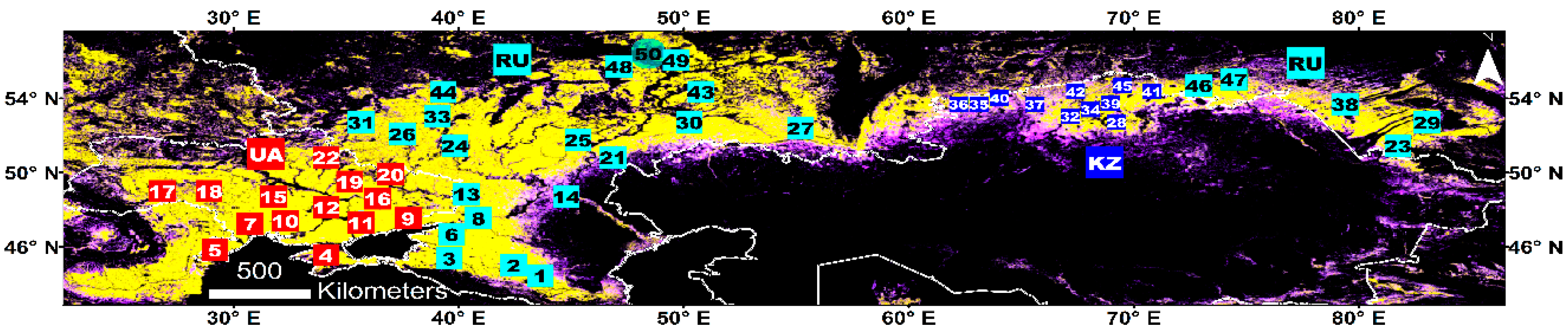
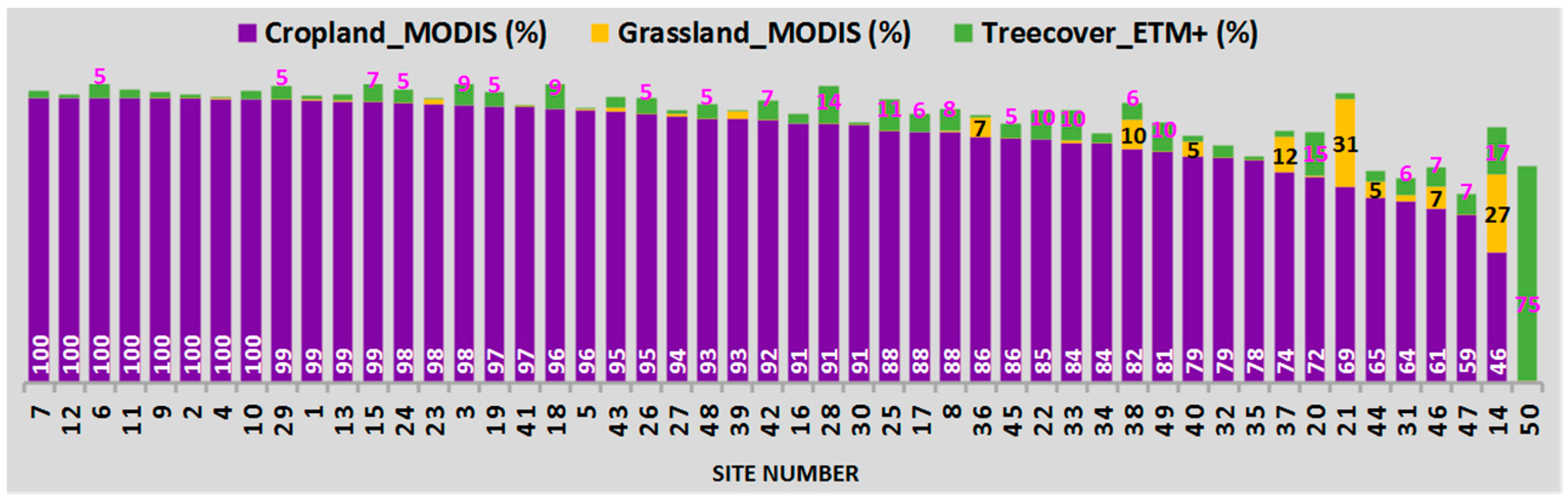
We used two very different remote sensing datasets: emitted terrestrial microwave radiation and reflected solar shortwave radiation. The microwave dataset was based on the Advanced Microwave Scanning Radiometer (AMSR-E) enhanced land parameters developed by the Numerical Terradynamic Simulation Group at the University of Montana [26]. These parameters include near surface air temperature (ta; ~2 m height) and vegetation canopy transmittance (tc) at three microwave frequencies (6.925 GHz, 10.65 GHz, and 18.7 GHz). Onboard the NASA-EOS Aqua satellite, AMSR-E recorded data twice daily (daytime, ~13:30; and nighttime, ~01:30) from mid-June 2002 to October 2011, when the rotating antenna failed. The second dataset included optical reflectance data from the Moderate-resolution Imaging Spectroradiometer (MODIS). We used MODIS collection 5 level 3 data product in a 0.05 degree (~5.6 km) Climate Modeling Grid (CMG), specifically the Nadir Bidirectional Reflectance Distribution Function (BRDF)-Adjusted Reflectance (NBAR) data that combines observations from Terra and Aqua (MCD43C4; [27]). NBAR provides 16-day retrievals (updated every 8 days) of surface reflectance normalized to a nadir view using BRDF models of surface anisotropy [28,29].
Croplands for this study were identified based on the International Geosphere Biosphere Programme (IGBP) global land cover classification scheme in the MODIS land cover CMG product (MCD12C1; [27]), and the USDA Foreign Agriculture Service (FAS) crop layers by oblast (for Russia [30], Kazakhstan [31], and Ukraine [32]).
We used tree cover data (ca. 2010) from the 30 m Global Land Cover dataset, which was derived from Landsat 7 ETM+ data by USGS and the Department of Geographical Sciences at University of Maryland [33]. We used these data to calculate the proportion of tree cover within our study sites.

2.2. Study Region

We conducted this study at the same sites identified in our companion paper [22] that established the notion that the surface air temperature data retrieved from the microwave radiometers could be used instead of MODIS land surface temperature data to drive the convex quadratic model of land surface phenology (LSP). Indeed, it improved model fits, despite its coarser spatial resolution, because there was higher temporal resolution and lower variability arising from the spatial heterogeneity of the land surface. In that paper, we used AGDD from AMSR-E air temperature data, and NDVI and EVI from MODIS data to characterize cropland dynamics throughout the growing season in the study region [22].
AMSR-E pixels dominated by croplands were identified through land cover stability analysis [22,34] using the MODIS IGBP Land Cover Type 1 Percentage Product (MCD12C1; [27]). We identified 49 AMSR-E pixels (or study sites) across the major grain producing areas of Ukraine (UA, 14), southern Russia (RU, 24), and northern Kazakhstan (KZ, 11) (Figure 1 and Figure 2; [22]). For contrast, we selected one AMSR-E pixel dominated by mixed forest cover (IGBP class 5) in Mari El Republic of the Russian Federation. We used this representative MFO site only for contrast and did not incorporate it into our full analyses. Where it is included, it is indicated in figure captions or accompanying text. We derived, within each study pixel, the proportions of croplands, grasslands, and cropland/natural vegetation mosaic (CNVM) using the MODIS IGBP Land Cover product (MCD12C1; [27]). These classes were the three predominant land covers in the region. In addition, we calculated the tree cover proportion from the Landsat 7 ETM+ 30 m resolution Global Land Cover data [33]. The proportions of tree cover, open water, bare ground, and undifferentiated other classes (including croplands and grasslands) that occur within each AMSR-E study pixel appear in Figure 2.
Over the eight years of the study period, the average cropland cover for all sites was 88%; in contrast, the mixed forest site was 93% mixed forest. Many sites in UA and some in RU had 100% average maximum cropland cover over the study period, while Volgograd (site 14) in RU had the minimum average cropland cover (46%, Figure 2). Saratov 1 in RU (site 21) had the largest grassland encroachment with 69% and 31% mean cropland and grassland cover, respectively, over the eight years (Figure 2). Thus, site 21 exhibited the largest cropland cover variation (range = 28%) [22]. Omsk 1 in RU (site 46), and Kostanay 2 in KZ (site 36) are other examples. The finer resolution Landsat data revealed that the MFO site (site 50) had the largest tree cover proportion (75%), followed by Volgograd (site 14, 17%).

2.3. Characterizing Land Surface Phenology in VODs and NDVI

We used the AMSR-E and MODIS data from all eight years (2003–2010) for all pixels. The AMSR-E data record has winter data gaps as it was pre-filtered for snow covered or frozen land surfaces [35]. To avoid the frozen season and to maintain a consistent analysis period across all pixels, we restricted our focus to data from DOY 89–305, i.e., 30 March to 1 November for non-leap years and 29 March to 31 October for leap years. An 8-day forward moving average filter was applied to the AMSR-E data to minimize data gaps due to orbit and swath width, and to align the AMSR-E data with the corresponding compositing periods of the MODIS NBAR data (MCD43C4) (Figure 3). Growing degree-day (GDD) is the daily thermal time increment above a certain threshold (base temperature) for plant growth [36,37,38], and accumulated growing degree-days (AGDD) are the summation of daily thermal time increments throughout the whole growing period [24,39,40]. In other words, the passage of days is weighted by the quantity of growing degrees occurring that day, with zero (but not negative) degrees being a permissible weight [41]. McMaster [42] concluded that the base temperature of 0 °C is a robust and sufficient threshold for wheat phenology, which is the main crop in our study region. GDD was calculated from the AMSR-E air temperature (ta) data with a base temperature of 273.15 K (=0 °C) as follows:
GDD = max [ t ASC + t DES 2 273.15 ,   0 ]
where tASC and tDES are ascending and descending pass temperatures, which roughly corresponds to the daytime (~13:30) and nighttime (~22:30) temperatures, respectively. We applied an 8-day forward moving summation to the GDDs and picked up those values corresponded with the MODIS reflectance data (MCD43C4) acquisition dates to mimic the whole growing season GDD (DOY 89–305 in this case) and to align it with the MODIS data. Thus, each annual growing period has 28 GDD values. These GDD values were accumulated to yield AGDD.
AGDDt = AGDDt−1 + GDDt
where GDDt is daily temperature increment of growing degree days at time t.
Daily GDD from AMSR-E tracked seasonal, weekly and monthly dynamics of corresponding weather station GDD [22]. The root mean square deviation (RMSD) between these daily datasets from the two sources was very low, 1.86–3.16 °C [22]. Linear regression of AMSR-E GDD with weather station GDD on these cropland sites yielded R2 > 0.82 [22]. This result is in line with Jones et al. [43] who found a bias of 1.0–3.5 K between WMO weather station and AMSR-E daily air temperature data on vegetated lands across the Northern Hemisphere.
NDVI was calculated from the MODIS NBAR reflectance data using the standard formula by Tucker [44]. NDVI was calculated for each 0.05-degree (~5.6 km) pixel and zonal-averaged to the 0.25-degree (25 km) AMSR-E study pixels. We fitted the MODIS NDVI as a function of AMSR-E AGDD using the downward CxQ model.
NDVIt = α + β × AGDDt – γ × AGDDt2
The intercept α is the background NDVI at the start of observation period, the linear parameter β affects the slope, and the quadratic parameter γ controls the curvature. Since the model is downward convex quadratic, the sign of β coefficient is positive and γ coefficient is negative.
Two phenometrics were derived from the fitted parameter coefficients of the CxQ model. These are Peak Height NDVI (PH; Equation (4)) and Thermal Time to Peak NDVI (TTPNDVI; Equation (5)):
PH = α − (β2/4 × γ)
TTPNDVI = −β /2 × γ
where α, β, and γ are the fitted parameter coefficients.
Vegetation Optical Depth (VOD) was derived as a negative natural logarithm of vegetation transmittance [VOD = −loge(tc) = −ln(tc)]. In a previous study [21], we fitted the core growing season VODs from the three microwave frequencies (6.925 GHz, 10.65 GHz, and 18.7 GHz) using the CxQ model in a two-step process. The fits in that study were good (coefficients of determination were larger than 0.90 (R2 > 0.90) in time and space) but limited to around the peak of the growing season. Here, however, we need to consider a larger fraction of the growing season; thus, we needed a different approach. The VOD shapes for the entire growing season are not well fitted using the CxQ model. VOD is sensitive to aboveground biomass structure, including crop residues, and to the vegetation water content found in entire aboveground biomass, while NDVI is sensitive primarily to vegetation greenness. VOD has a different seasonal progression shape that is not suitably captured by a quadratic curve compared to that of NDVI. Therefore, we used the maximum VOD value approach to determine cropland vegetation PH and TTP. That is, the observed maximum VOD value was taken as PH VOD, while the corresponding AGDD was taken as TTP. Similar approach was also used for the NDVI for a direct comparison with the CxQ model fit derived PH and TTP NDVI. The PH NDVI and PH VOD values were regressed to see the relationship between cropland peak greenness and peak biomass and water content. We then used analysis of covariance (ANCOVA) to test whether the slopes and/or intercepts from the linear regression model fit were significantly different by microwave frequency: the microwave frequencies (6.925, 10.65, and 18.7 GHz) were the independent categorical effect variables, the peak greenness was covariate, and PH VOD was the response variable. The first statistical assumption for ANCOVA is that the covariate (peak greenness in our case) is uncorrelated with other independent variables (microwave frequencies), and the second assumption is that the covariate (peak greenness) is correlated with the dependent variable (PH VOD; [45]). In all cases, p ≤ 0.05 was considered significant.

3. Results

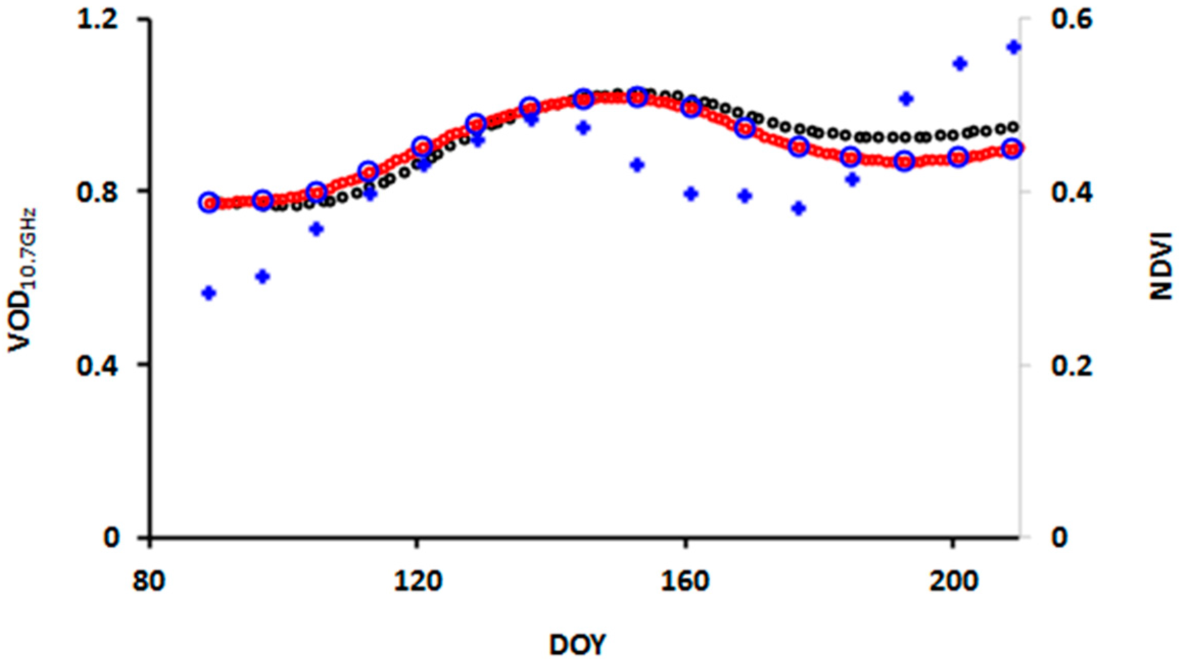
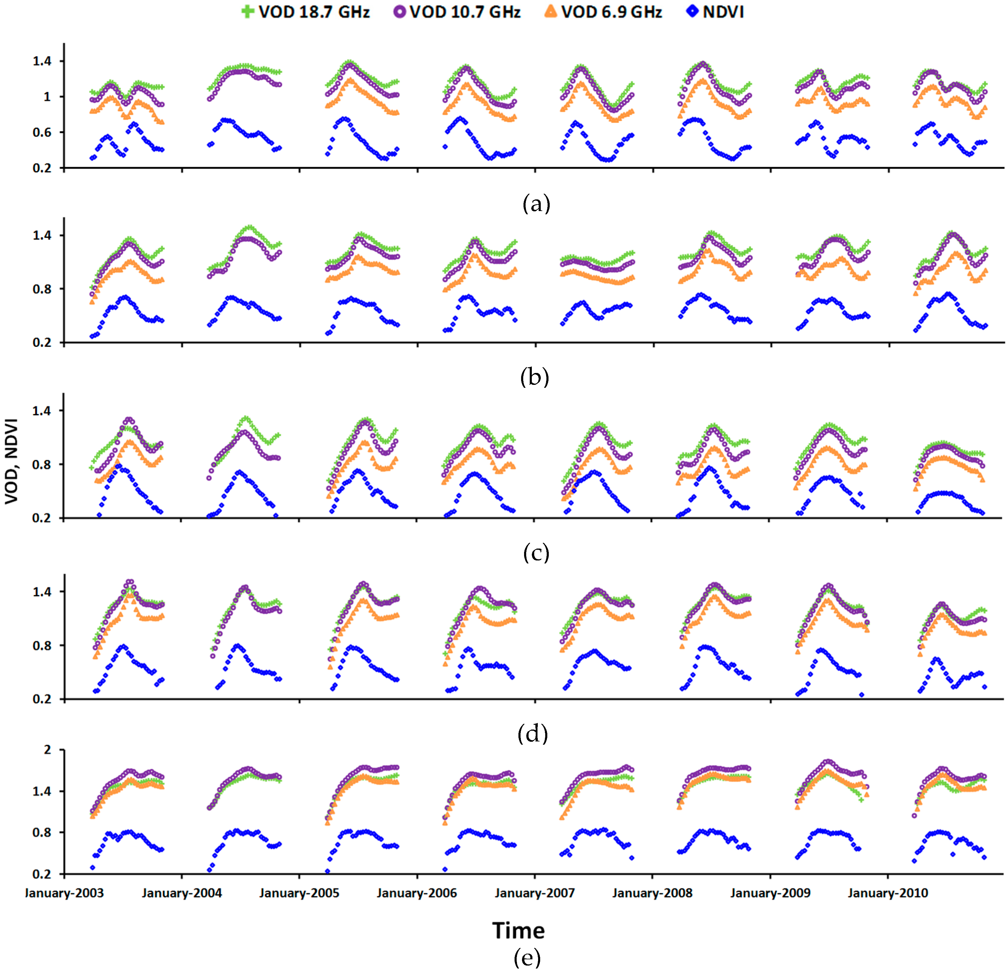
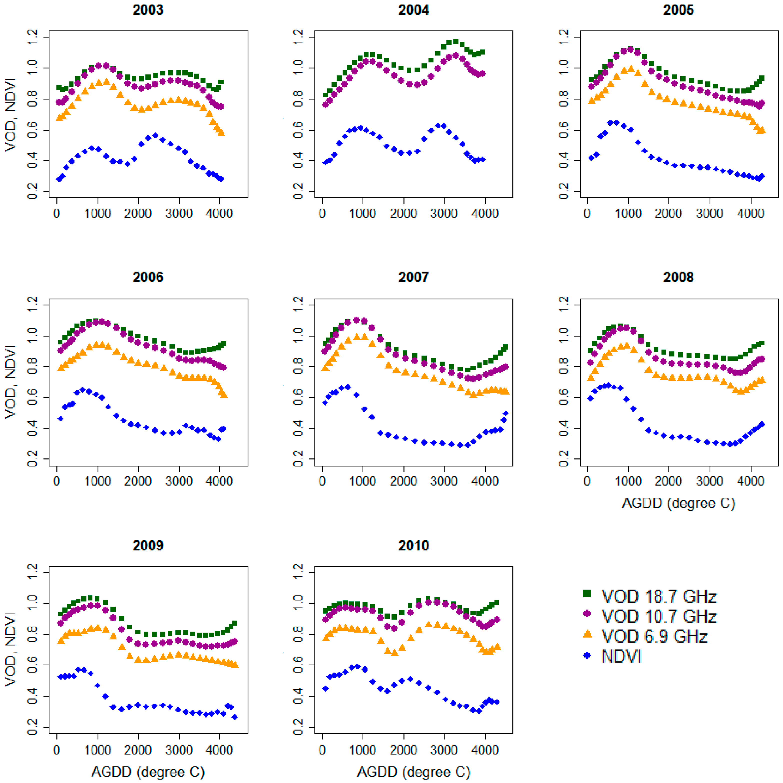
3.1. Time Series Land Surface Phenologies of NDVI and VODs

All three VOD time series were able to capture the seasonality of croplands (both bimodal patterns and unimodal patterns), similar to MODIS NDVI (Figure 4). The bimodality arises from the planting of winter grains in the fall, and growth and harvest in the subsequent early summer. After snow melts, croplands are primarily barren or contain crop residues (non-photosynthetic biomass) prior to tilling and planting. Green-up occurs after seed germination at emergence (initiation of visible aboveground growth) but prior to significant aboveground biomass accumulation. This pattern is evident in Figure 4 and Figure 5, where the rise in VOD occurs later than NDVI. Cropland peak VODs, which are sensitive to aboveground vegetation water content and biomass, consistently lagged in time and space from the peak NDVI, which is sensitive to vegetation greenness and leaf area index (Figure 4 and Figure 5). Furthermore, the VODs showed slower senescence, likely a consequence of residual biomass (crop residue) following harvest. VOD PH for sites with ≥10% tree cover were not significantly different from sites with ≥99% croplands at α = 0.05 and p > 0.05 (Figure 4 and Figure 5) [46,47]. Higher microwave frequencies exhibit higher dynamic range: the shorter wavelengths are more attenuated by vegetation canopy (Figure 4 and Figure 5).
LSPs at the lower latitudes within the region exhibit longer and/or bimodal patterns arising from the cultivation of winter grains (Figure 4a,b). On the other hand, LSPs at the higher latitudes exhibit shorter unimodal growing season due to cultivation of spring grains (Figure 4c,d). At each study site, the VOD and NDVI exhibit similar seasonal patterns, amid interannual variation. For example, in Petropavlovsk 3, KZ (Figure 4c), in 2003 there was high and earlier peak LSPs in fewer AGDD, while in 2010 there was lower and flatter peak in more AGDD, due to the 2010 heatwave affecting European Russia [19,20]. Note the 2007 VOD in Kirovohrad, UA (Figure 4b) is almost flattened compared to other years, due to the devastation of crops by the 2007 heatwave in Ukraine [48]. The heatwave effect is more evident on the VODs compared to their counterpart NDVI (Figure 4b), due to the sensitivity of VODs to vegetation water content. The Mari El mixed forest site in Russia displayed a distinct LSP in magnitude and shape compared to the rest of the 49 cropland sites (Figure 4e). Both VOD and NDVI were larger in magnitude (note the y-scales) and flatter in shape. The VODs in particular showed a much-delayed senescence compared to the NDVI. The magnitude and peak timing of VOD were found sensitive to woody plant foliage, whereas NDVI seasonality was governed by the green herbaceous vegetation [49,50,51].
Figure 5 shows Time series of VODs and NDVIs in a southern study site (Simferopol, UA) that experienced alternate unimodal and bimodal seasonal patterns over the eight years. All three microwave frequencies VOD were able to capture these LSP patterns similar to their counterpart NDVI, despite some differences in magnitude and shape.

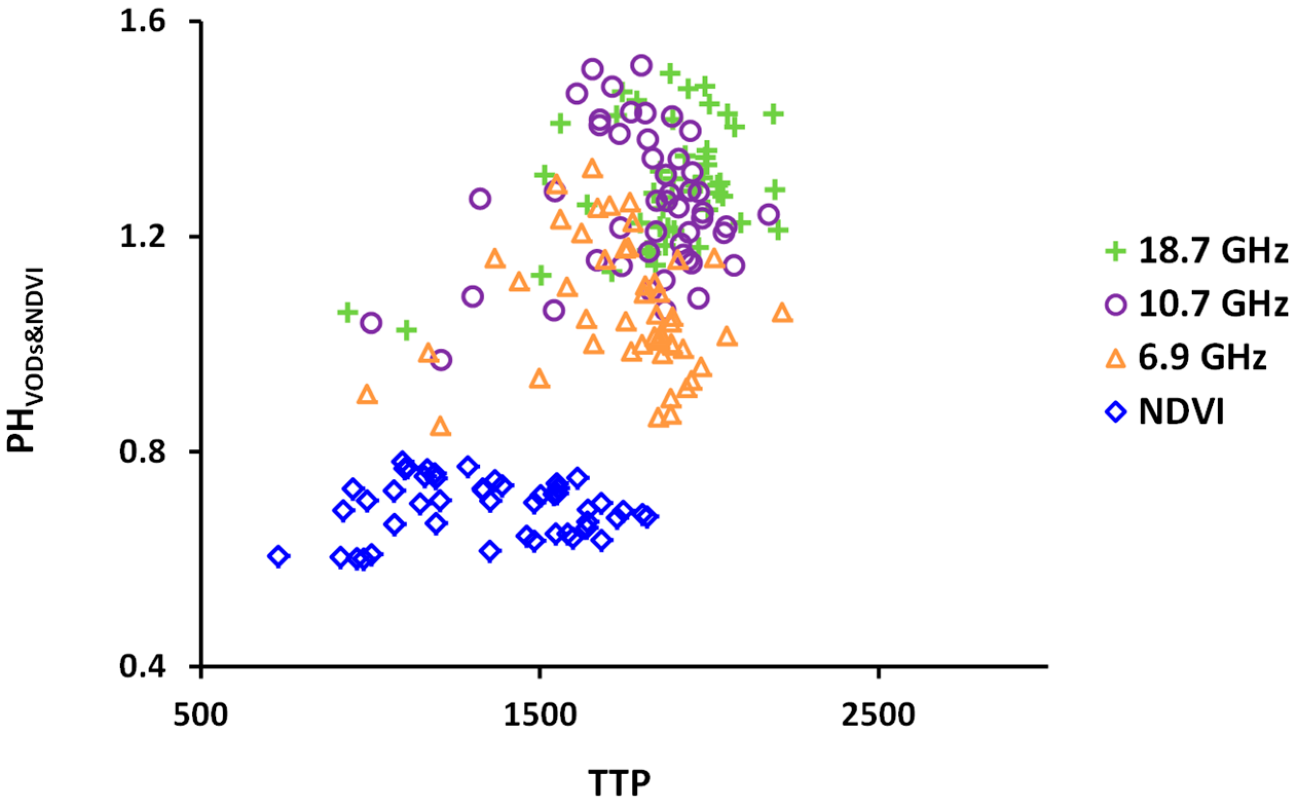
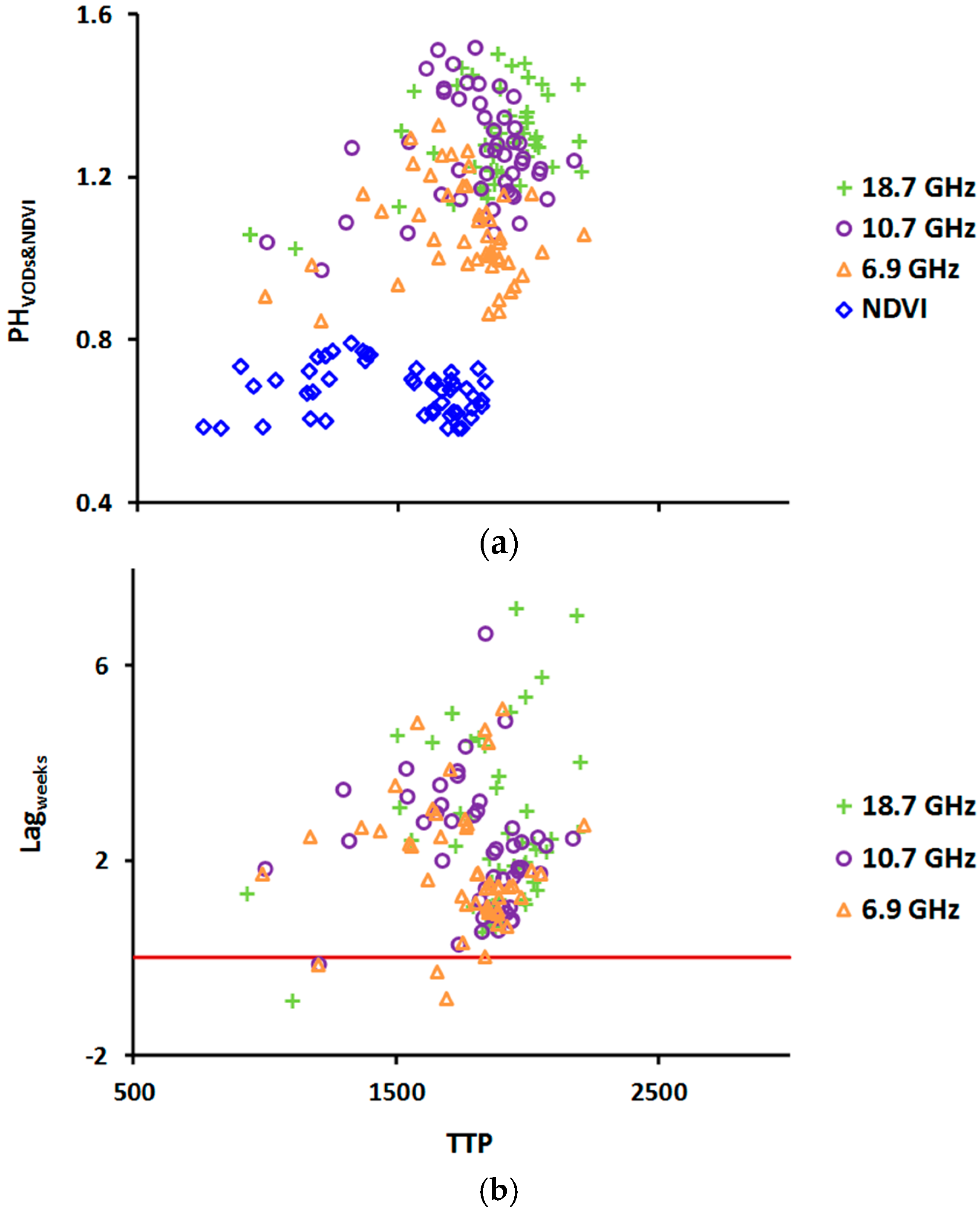
3.2. Thermal Time to Peak and Peak Height NDVI and VOD Phenometrics

In this section, we present TTPNDVI and PHNDVI derived from the CxQ model, followed by nonparametric phenometrics for VOD and NDVI determined from the growing season maxima.

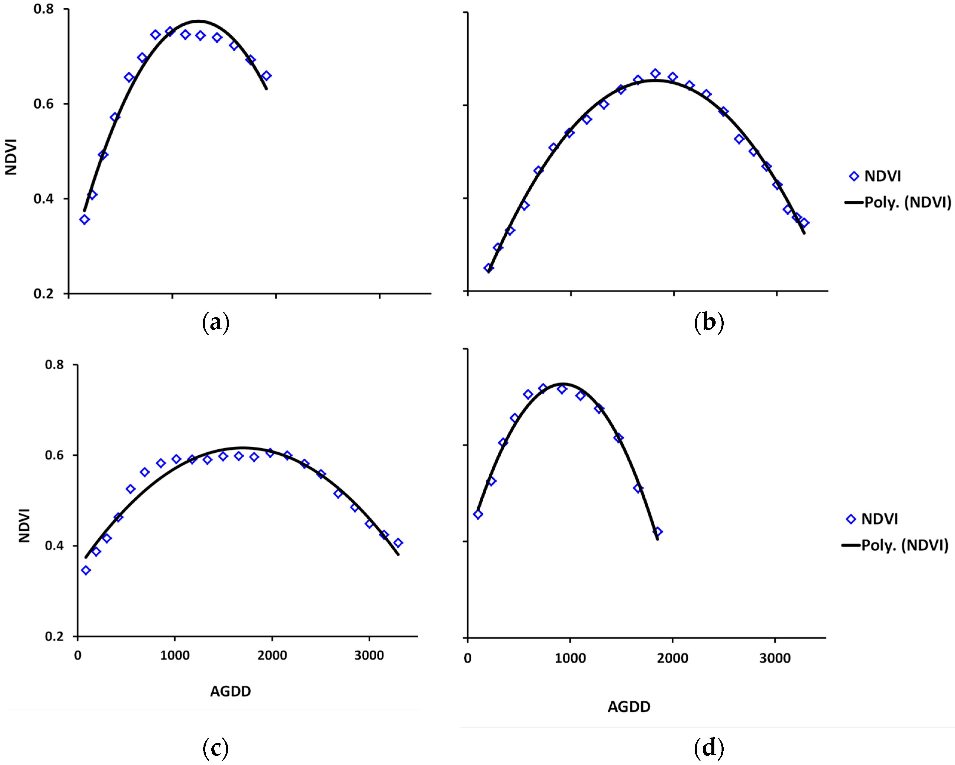
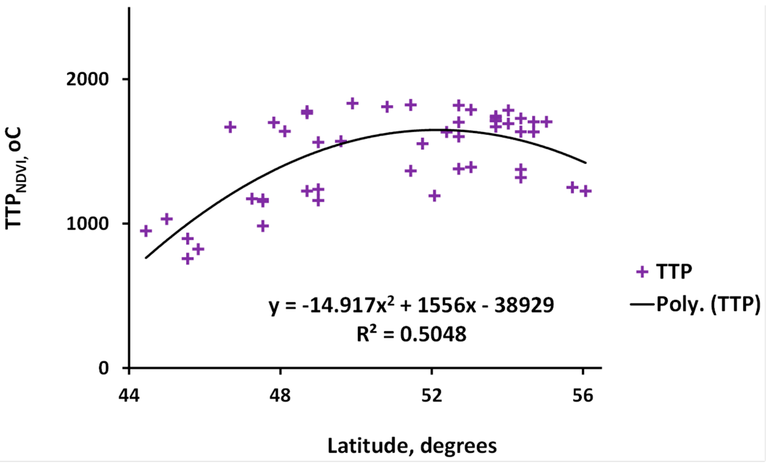
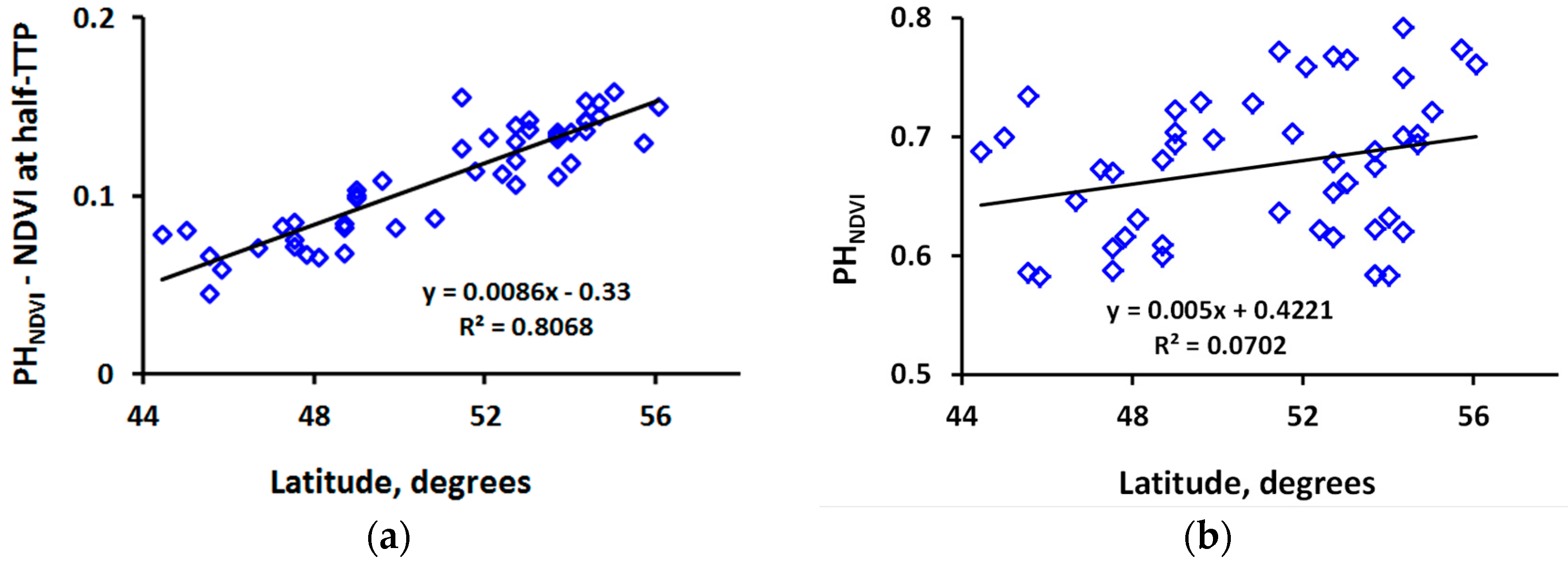
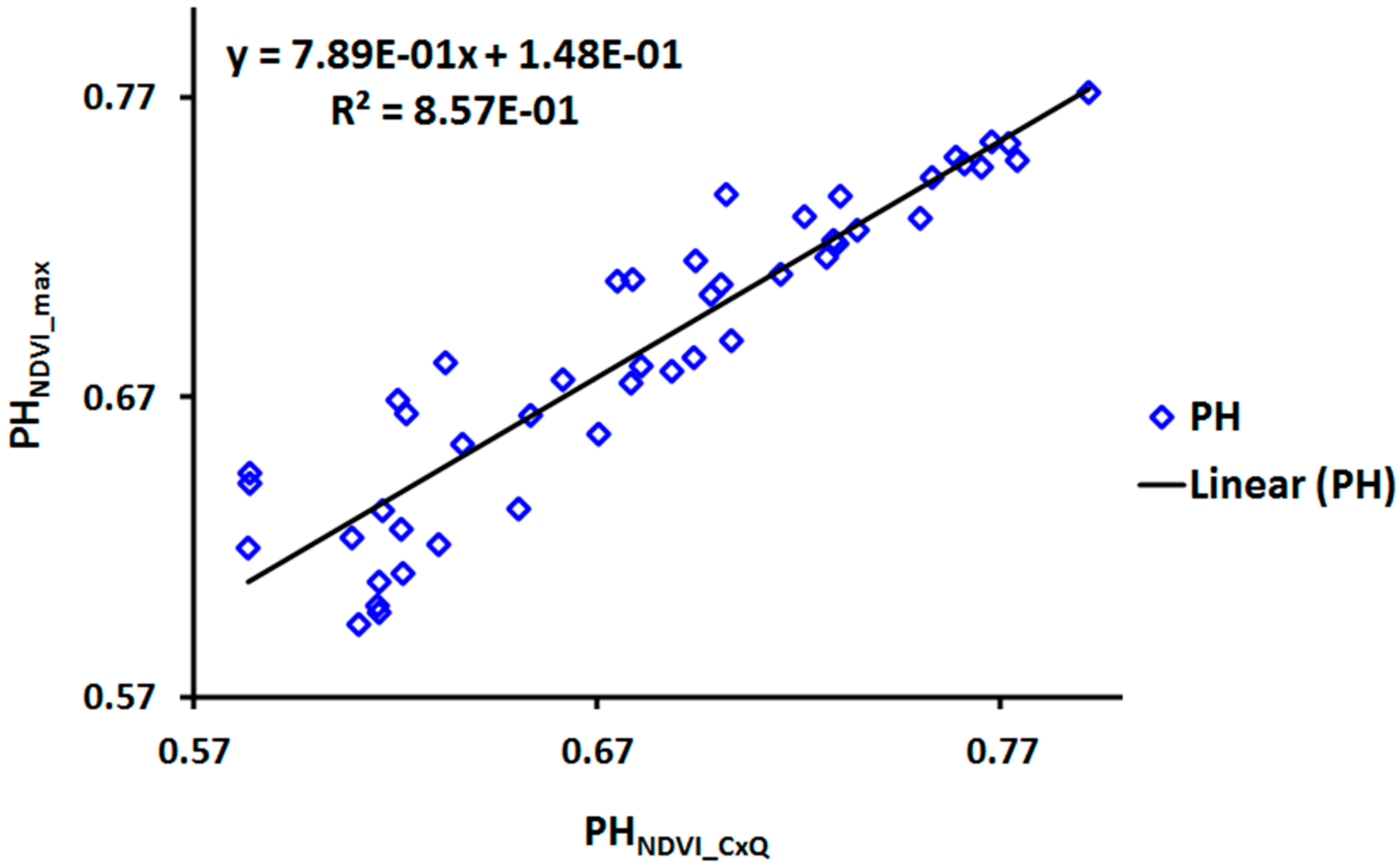
3.2.1. The CxQ Model Derived NDVI Phenometrics

The NDVI CxQ model fits for all sites are high with 0.78 < R2 < 0.99. Sample fits appear in Figure 6. Sites at lower latitudes that can support double growing season attain their first peaks at the earliest (<1000 AGDD, e.g., Figure 6d, Cherkessk, RU, 44°); moving farther north, the seasonal pattern shifts from bimodal to unimodal, and the TTPNDVI is pushed up further to the growing season (between 1000 and 2000 AGDD, e.g., Figure 6c, Zaporiyhzhya 1, UA, 48° and Figure 6b, Kokshetau 1, KZ, 53°). Moving towards the northern study sites, the TTP starts to decrease to 1000 AGDD due to the thermal limitation and shorter growing season (e.g., Figure 6a, Cheboksary, RU, 56°). Figure 7 presented the general relationship of TTPNDVI as a function of latitude for all sites. Note also the NDVI CxQ fit intercept in the different latitudes in Figure 6 that the growing season in the lower latitudes (e.g., Figure 6d) starts a bit earlier than the time we considered in this study (DOY 89 = March 30 (March 29 in leap years)).
Average (2003–2010) PHNDVI phenology metric in our study croplands ranged between 0.58 and 0.84 (not shown here). NDVI at half-TTP (NAHT) as a function of PHNDVI displayed a distinct trend indicating that NDVI in these sites is driven by local climate (Figure 8a). Generally, lower latitude study sites have gentler NDVI gradient time series with longer growing season compared to the steeper NDVI gradient of the shorter summer growing season at higher latitudes. Thus, the difference between PHNDVI and NDVI at half-TTP increased as latitude increases, yielding a strong linear fit with R2 = 0.81 (Figure 8a). However, the PHNDVI as a function of latitude did not show a clear trend (Figure 8b). Temperature dominates crop growth from spring to summer, while other variables (such as rainfall) play roles that are more important in crop production.
The NAHT as a function of PHNDVI, for selected sites that were more impacted by the 2003, 2007, and/or 2010 heatwaves, showed a positive correspondence (Figure 9b). The two phenometrics for the mixed forest in the most northern study site Mari El, Russia (site 50 appears as the outlying green circles in upper right corner) displayed strong correspondence with R2 = 0.94. In contrast, the correspondence between these phenometrics for croplands exhibited more interannual variability. due to the fact that crops are annual vegetation and due to possible crop and land rotation annually or every few years. Moreover, croplands are more vulnerable to climatic variability compared to the perennial mixed forests. The southern study sites exhibited smaller NAHT and PHNDVI in 2003 due to minimal effect of the European heatwave on croplands in the study area [52]. As the winter grains were affected many croplands were sown to spring grains and, therefore, many southern study croplands in 2003 exhibited the double seasonality. The affected winter croplands (first peak) exhibit smaller NAHT and PHNDVI (Figure 9b sites 1, 2, 4, and 13). However, the smaller values for the two phenometrics were recorded in 2010 for the northern study sites, due to the effect of the 2010 Russian heatwave, which also impacted northern Kazakhstan (Figure 9b, sites 13, 24, and 36) [19,20]. As forests are perennial and resilient to climatic variability, the two phenometrics in Mari El, Russia were not that affected by the 2010 Russian heatwave and displayed closer values consistent trend throughout the study period. The 2010 NAHT as a function of PHNDVI for this mixed forest site was just about at an average position of the other seven years of values (Figure 9b).

3.2.2. The Maximum Value Approach for VOD Phenometrics

For the land surface phenology of VOD, Figure 10 presents the PHVOD as a function of the corresponding TTPVOD for all sites. In the study sites dominated by croplands, PHVOD ranged between 0.85 and 1.74, while the PHNDVI (also calculated using the maximum value approach) ranged between 0.60 and 0.83. The ordering of the PHVOD magnitude from high to low was 18.7 GHz > 10.65 GHz > 6.925 GHz: the higher the frequency, the higher the attenuation by vegetation, and, thus, the larger the VOD magnitude. The PHVOD lags the PHNDVI, because the PHVOD responds to vegetation water content and aboveground biomass, which both continue to increase after the apparent peak absorption of photosynthetically active radiation, which is captured by the PHNDVI. Generally, the shorter the microwave wavelength, the later the PHVOD occurs in terms of AGDD. The lag between the PHVOD for 10.65 and 18.7 GHz was narrower than between the PHVOD for 6.925 GHz from the other two. We have presented a quantified lag graph (Figure 11b) among the maximum value determined PH VODs and the CxQ model derived PH NDVI in Section 4.1.

4. Discussion

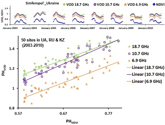
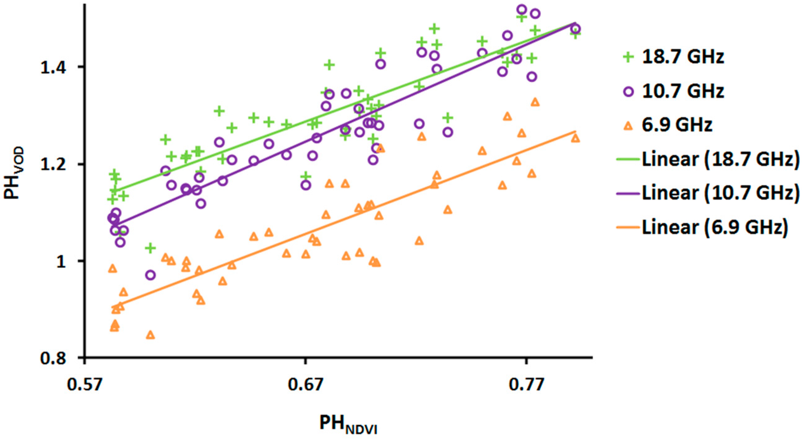
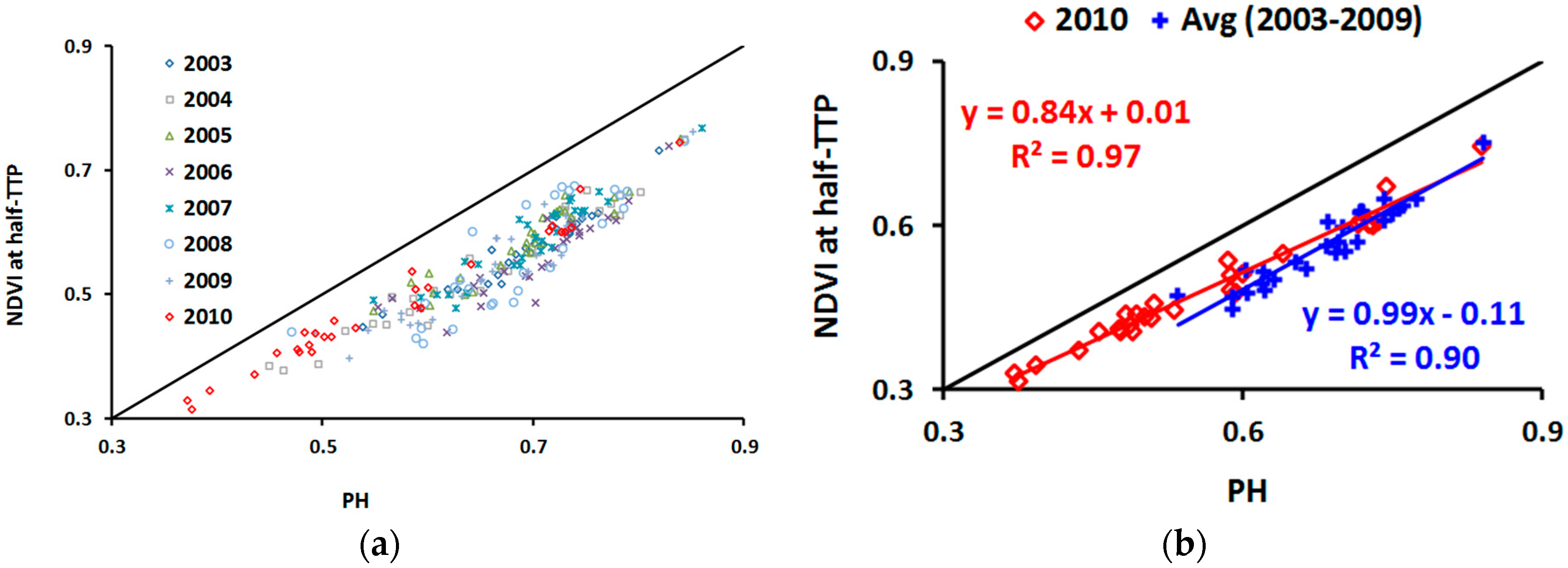
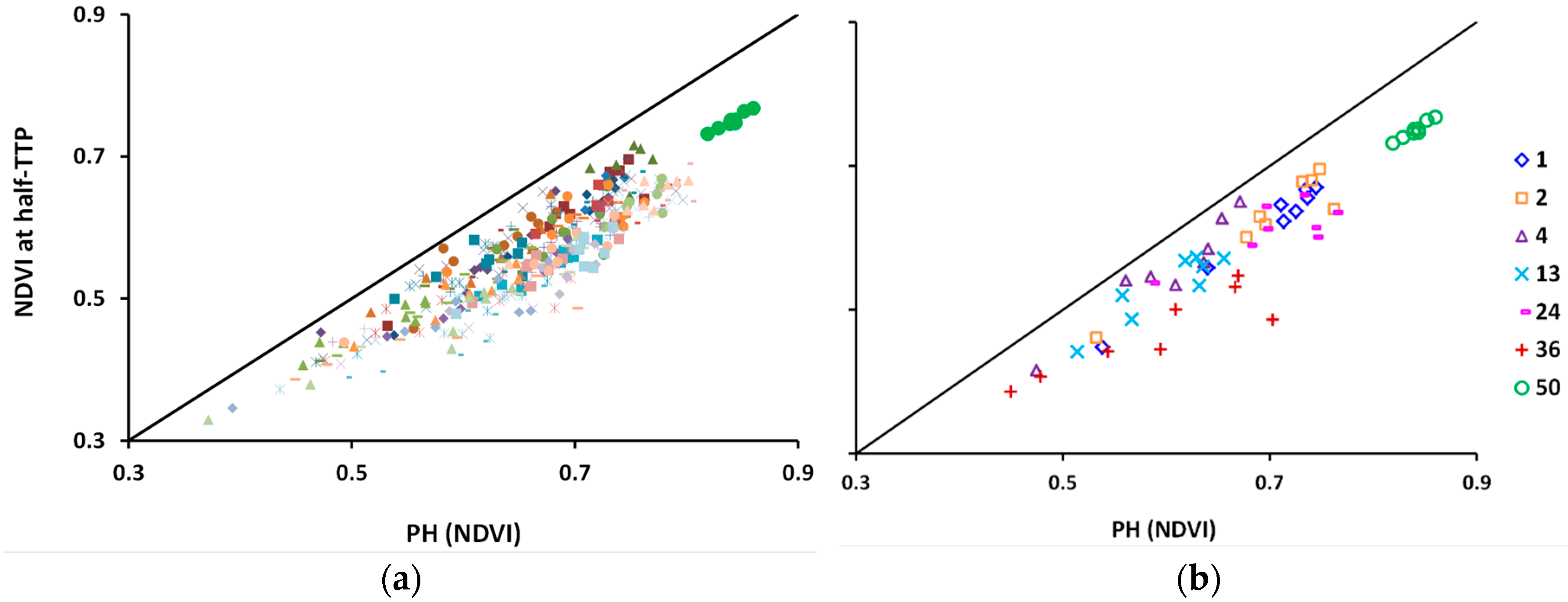
4.1. VOD and NDVI Peak Heights: Correlations and Biases

Peak heights are less likely to be affected by snow and other non-vegetation related issues compared to the start-of-season (SOS) [23,24]. PHNDVI has significant positive correlation to agricultural production [25]. The PHVOD derived using the maximum value approach corresponded favorably with the PHNDVI derived using the CxQ model. The 10.65 GHz PHVOD achieved the highest correspondence with the PHNDVI with a high coefficient of determination (R2 = 0.84) and the lowest standard error (SEE = 0.1275; Table 1, Figure 11). PH for the eight years’ average VOD and NDVI for all cropland sites except Saratov 1 (which had a significant proportion (31%) of grassland), were considered in this analysis.
Two hypotheses were tested using analysis of covariance (ANCOVA). First, the covariate (peak greenness) was not significantly (at α = 0.05) correlated to the independent variable (microwave frequency) [45]. ANCOVA revealed the slopes resulting from the linear fits between PHNDVI and PHVOD did not differ significantly between pairs of microwave frequencies (Table 2). The intercepts were significantly different, given the different magnitudes of the VODs. On global, annual scales, AMSR-E VOD was found more highly correlated with MODIS VI’s compared to anther passive microwave data, Soil Moisture and Ocean Salinity (SMOS) VOD did with the MODIS VI’s [53]. Second, the covariate PHNDVI was correlated with response variable PHVOD as described in the previous paragraph and in Table 1 and Figure 11 [45]. The interpretation from the fulfilment of these two ANCOVA assumptions is that peak greenness (PHNDVI) had a significant and positive effect on PHVOD and the effect is similar for all three microwave frequencies (the effect of PHNDVI on PHVOD did not depend on microwave frequency).
Even though PHNDVI and PHVOD have significant positive correspondence, the latter lagged the former (Figure 12b). This behavior was expected since microwaves are differentially sensitive to aboveground biomass and canopy water content; in contrast, the VNIR is differentially sensitive to photosynthetically active radiation (PAR) absorption. The peak VOD lags the peak greenness by several weeks following delayed increases in vegetation water content and development of aboveground biomass. Average VOD lag for all study years and sites was about three weeks, but it varied in time and space, and by microwave frequency (Figure 12b). We have also presented the PHVOD and PHNDVI as a function of their respective TTP metric in Figure 12a for ease of interpretation of the lags in Figure 12b. The temporal and spatial average PHVOD lag increases as microwave frequency increases. The 6.925, 10.65, and 18.7 GHz PHVOD average lags are 1.9, 2.2 and 2.7 weeks, respectively, relative to the peak greenness (Figure 12b and Table A1). PHNDVI lags PHVOD 6.925 GHz at three sites only. Few sites that showed PHNDVI temporal average lag to that of the PHVOD—three sites for the 6.925, one site for the 10.65 and one site for the 18.7 GHz PHVOD over the study period (all lags less than a week). Across the 50 sites the average temporal lag of PHVOD relative to PHNDVI ranges from −0.8 to +5.1 weeks for 6.925 GHz, from −0.1 to 6.7 weeks for 10.65 GHz, and from −0.9 to 7.2 weeks for 18.7 GHz.
To check the usefulness of the maximum value-based PH phenometrics determination approach, we correlated PHNDVI determined using this approach with that of the CxQ model. The PHNDVI from the two methods showed a strong linear relationship with an R2 of 0.86 (Figure 13). However, the CxQ model derived peak greenness lags the maximum-value determined peak greenness. On average, the CxQ model derived PHNDVI lags the maximum-value determined PHNDVI by one week. Therefore, there was a general underestimation of the PHVOD lags by about one week. On an ecoregional scale, studying AMSR-E SOS and MODIS green-up onset dates in North America, Jones et al. [1] found a correspondence between VOD SOS and green-up onset dates with R2 = 0.45 for VOD and NDVI, and R2 = 0.48 for VOD and LAI. In cropland dominated ecoregions (63% cropland) in North America, VOD SOS lagged by 5.7 to 12.9 weeks (mean = 8.6) compared to the NDVI green-up onset date [54].

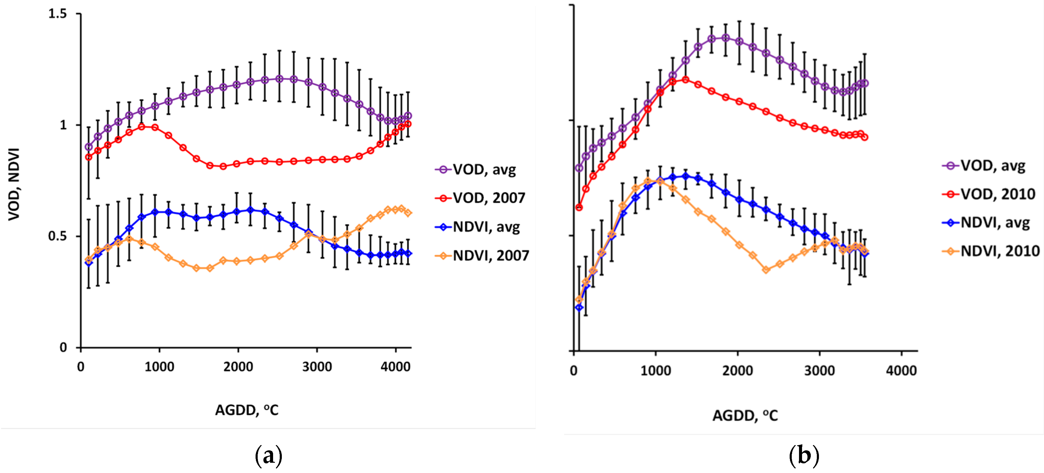
4.2. Heatwave Responses of VODs and NDVI

In our previous work [21,22], we have noted the 2010 heatwave affecting Russia and Kazakhstan [19,20] and the 2007 heatwave affecting Ukraine [48]. Here, the heatwave effects on croplands were revealed by the time series of VODs and NDVIs, the relative comparison of the two LSP measures, and the model derived phenometrics PHNDVI and NAHT. During the heatwave years, the VODs and NDVIs were well below the average VOD and NDVI for non-heatwave years, as croplands were negatively impacted by the excess heatwave (Figure 14). Heatwave years were more evident in the VODs compared to their counterpart NDVIs, since VOD strongly responds to vegetation water content. The difference of the VOD data during the heatwave years to the average non-heatwave years VOD was found significantly different (p < 0.001) from that of the similarly analyzed NDVI data (Figure 14). The CxQ model derived NAHT as a function of PHNDVI for sites affected by the 2010 heatwave was lower relative to the other non-heatwave years (Figure 15a). The difference between the PHNDVI and NAHT for the 2010 data was found significantly different (p < 0.001) from the average of the 2003–2009 data (Figure 15b). The marker in the upper-right corner of figure 15a is the mixed forest site in Mari El, Russia, showing little effect of the heatwave at that site.

5. Conclusions and Recommendations

In this paper, we have compared and contrasted the peak timing of cropland vegetation maturity using two complementary remote sensing datasets. Time series of LSP of VOD at three microwave frequencies—6.925, 10.65, and 18.7 GHz—from the passive Advanced Microwave Scanning Radiometer on EOS (AMSR-E) was able to capture the seasonality of croplands (both bimodal and unimodal seasonal patterns) similar to but different from that of the VNIR MODIS NDVI. A higher microwave frequency generates a higher VOD, since smaller wavelengths are more quickly attenuated by aboveground vegetation.
The timing and magnitude of the growing season peak (TTP and PH) are more consistent quantitative cropland phenometrics, in large part because they are minimally affected by snow or frost, unlike the commonly-used but ill-defined phenometrics of Start of Season and End of Season. The vegetation optical depth (VOD) retrieved from passive microwave data appears to be more robust to atmospheric effects and biomass saturation than the phenometrics based on the NDVI.
We have also demonstrated the application of the downward convex quadratic (CxQ) function to model cropland dynamics using MODIS NDVI yielding strong fits (0.78 < R2 < 0.99). However, the shape of the VOD time series curve shape was more complicated than a simple quadratic fit. The passive microwave AMSR-E PHVOD determined using the growing season maximum value of the growing season approach favorably corresponded with that of the VNIR MODIS peak greenness (PHNDVI) derived using the CxQ model over the study domain with R2 between 0.77 and 0.84. Although the 10.65 GHz PHVOD exhibited the best linear regression fit (R2 = 0.84) and with lowest standard error (SEE = 0.128) with the PHNDVI, the ANCOVA model analysis revealed that the slopes resulting from the linear regression fits were not significantly different by microwave frequency. In contrast, the intercepts from the ANCOVA analysis were significantly different: not surprising given the different dynamic ranges of the VODs.
Despite the strong correspondence between peak LSPs of the two datasets, there was a general lag of AMSR-E PHVOD by two weeks compared to that of MODIS PHNDVI. Based on PHNDVI analysis of same dataset using the two procedures, we found a one-week bias between the two methods, translating into a lag of three weeks between PHNDVI and PHVOD. We conclude that maximum value based PHVOD can yield phenometrics complementary to the model based PHNDVI, especially in cloud and aerosol obscured parts of the world.
The unsuitability of the CxQ model for characterizing the VOD curves and deriving simple phenometrics limits the generalizability of the CxQ model. Moreover, determining the PHVOD phenometrics using the seasonal maximum value could introduce error, when maxima result from noise. With this caveat and keeping the lag, we find the passive microwave PHVOD to complement well the VNIR PHNDVI. However, further research is needed to evaluate how best to use this complementarity for monitoring cropland dynamics and forecasting agricultural crop production, particularly in data sparse, cloud-obscured, and food-insecure parts of the world.
Although the AMSR-E ceased to function in October 2011 due to antenna failure, its legacy has been continued since May 2012 by AMSR2, an improved version of AMSR-E but with similar functionality since May 2012 [55]. A new blended passive microwave dataset spans the gap between the two sensors by the Microwave Radiation Imager (MWRI) sensor data on-board the Chinese FengYun 3B (FY3B) satellite [55,56]. Our next step is to evaluate the use of these passive microwave data to characterize the croplands dynamics in cloud-obscured East Africa and explore linkages to agricultural crop production.

Acknowledgments

This research was supported in part through the NASA Earth and Space Sciences Fellowship program (NNX13AN58H), and the NASA LCLUC (NNX11AB77G) and Science of Terra and Aqua (NNX14AJ32G) programs. The AMSR-E data were accessed from Numerical Terradynamic Simulation Group (NTSG) website (www.ntsg.umt.edu/project/amsrelp). The MODIS data were obtained from the NASA/USGS Land Processes Distributed Active Archive Center (LP DAAC) (https://lpdaac.usgs.gov/products/modis_products_Table). Thanks especially to John Kimball for his continuing advice.

Author Contributions

W.G.A. and G.M.H conceived and designed the experiments; W.G.A. performed the experiments; W.G.A. and G.M.H. analyzed the data; and W.G.A. and G.M.H. wrote the paper.

Conflicts of Interest

The authors declare no conflict of interest.

Appendix A

Table A1. Study sites average GDD, and PH VOD lags (in weeks) relative to PHNDVI (Figure 11).
Site No.NameLatitudeLongitudeLag, 6.9 **Lag, 10.7 **Lag, 18.7 **Site No.NameLatitudeLongitudeLag, 6.9 **Lag, 10.7 **Lag, 18.7 **
1Cherkessk, RU44.443.52.72.44.426Kursk, RU52.137.55.13.87.0
2Stavropol, RU45.042.42.63.33.127Orenburg, RU52.455.21.41.21.1
3Krasnodar, RU45.639.64.86.77.228Kokshetau 1, KZ52.769.22.72.52.6
4Simferopol’, UA45.634.11.71.81.329Barnaul 2, RU52.783.01.01.71.9
5Tulcea, UA45.829.22.53.54.630Kuybyskev 2, RU52.750.21.12.34.0
6Rostov-on-Don 2, RU46.739.81.52.52.331Orel, RU52.735.72.72.93.5
7Odesa, UA47.330.73.13.74.432Kokshetau 2, KZ53.067.41.71.71.6
8Rostov-on-Do 1, RU47.540.94.73.54.533Lipetsk, RU53.039.11.62.02.3
9Donets’k, UA47.537.73.63.95.034Kokshetau 3, KZ53.768.20.90.81.2
10Mykolayiv, UA47.532.34.44.95.435Kostanay 1, KZ53.763.31.00.90.7
11Zaporiyhzhya 1, UA47.835.7−0.30.31.136Kostanay 2, KZ53.762.20.90.50.5
12Zaporiyhzhya 2, UA48.134.11.42.42.437Kurgan, KZ53.765.61.51.01.0
13Luhans’k, RU48.740.40.71.00.638Barnaul_1, RU53.779.41.51.61.9
14Volgograd, RU48.744.8−0.1−0.1−0.939Kokshetau 4, KZ54.069.01.11.81.9
15Kirovohrad, UA48.731.81.81.02.240Kostanay 3, KZ54.064.01.30.90.7
16Kharkiv 2, UA49.036.21.82.22.641Petropavlovsk 2, KZ54.470.81.52.32.4
17Khmel’nyts’kyz, UA49.026.83.94.34.442Petropavlovsk 3, KZ54.467.41.11.41.6
18Vinnytsya, UA49.028.92.33.15.843Kuybyskev 1, RU54.450.82.83.02.8
19Poltava, UA49.635.11.32.73.044Ryazan, RU54.439.32.52.83.0
20Kharkiv 1, UA49.937.00.00.81.145Petropavlovsk 1, KZ54.769.51.51.71.8
21Saratov 1, RU50.846.90.1−0.3−0.746Omsk 1, RU54.772.91.31.92.2
22Sumy, UA50.834.1−0.80.61.247Omsk 2, RU55.074.50.31.82.0
23Semipalatinsk, RU51.481.70.60.81.448Cheboksary, RU55.747.13.03.05.1
24Voronezh, RU51.439.82.93.23.749Kazan’, RU56.149.52.32.82.4
25Saratov 4, RU51.845.31.72.22.050Mari El *56.448.4−0.74.76.9
Max * 5.16.77.2
Min * −0.8−0.1−0.9
Average * 1.92.22.7
* excludes Saratov 1 and Mari El. ** lags have not been adjusted to account for the methodological bias described in Section 4.1.

References

  1. Jones, M.O.; Kimball, J.S.; Jones, L.A.; McDonald, K.C. Satellite passive microwave detection of North America start of season. Remote Sens. Environ. 2012, 123, 324–333. [Google Scholar] [CrossRef]
  2. Henebry, G.M.; de Beurs, K.M. Remote sensing of land surface phenology: A prospectus. In Phenology: An Integrative Environmental Science; Schwartz, M.D., Ed.; Springer Netherlands: Dordrecht, The Netherlands, 2013; pp. 385–411. [Google Scholar]
  3. Schwartz, M.D.; Hanes, J.M. Intercomparing multiple measures of the onset of spring in eastern North America. Int. J. Climatol. 2010, 30, 1614–1626. [Google Scholar] [CrossRef]
  4. Wang, Q.; Tenhunen, J.; Dinh, N.Q.; Reichstein, M.; Otieno, D.; Granier, A.; Pilegarrd, K. Evaluation of seasonal variation of MODIS derived leaf area index at two european deciduous broadleaf forest sites. Remote Sens. Environ. 2005, 96, 475–484. [Google Scholar] [CrossRef]
  5. Frolking, S.; Milliman, T.; McDonald, K.; Kimball, J.; Zhao, M.; Fahnestock, M. Evaluation of the seawinds scatterometer for regional monitoring of vegetation phenology. J. Geophys. Res. Atmos. 2006, 111, D17302. [Google Scholar] [CrossRef]
  6. Jones, M.O.; Jones, L.A.; Kimball, J.S.; McDonald, K.C. Satellite passive microwave remote sensing for monitoring global land surface phenology. Remote Sens. Environ. 2011, 115, 1102–1114. [Google Scholar] [CrossRef]
  7. Min, Q.; Lin, B. Determination of spring onset and growing season leaf development using satellite measurements. Remote Sens. Environ. 2006, 104, 96–102. [Google Scholar] [CrossRef]
  8. Shi, J.; Jackson, T.; Tao, J.; Du, J.; Bindlish, R.; Lu, L.; Chen, K.S. Microwave vegetation indices for short vegetation covers from satellite passive microwave sensor AMSR-E. Remote Sens. Environ. 2008, 112, 4285–4300. [Google Scholar] [CrossRef]
  9. Frolking, S.; Fahnestock, M.; Milliman, T.; McDonald, K.; Kimball, J. Interannual variability in North American grassland biomass/productivity detected by seawinds scatterometer backscatter. Geophys. Res. Lett. 2005, 32, L2140. [Google Scholar] [CrossRef]
  10. Frolking, S.; Milliman, T.; Palace, M.; Wisser, D.; Lammers, R.; Fahnestock, M. Tropical forest backscatter anomaly evident in seawinds scatterometer morning overpass data during 2005 drought in Amazonia. Remote Sens. Environ. 2011, 115, 897–907. [Google Scholar] [CrossRef]
  11. Kimball, J.S.; McDonald, K.C.; Running, S.W.; Frolking, S.E. Satellite radar remote sensing of seasonal growing seasons for boreal and subalpine evergreen forests. Remote Sens. Environ. 2004, 90, 243–258. [Google Scholar] [CrossRef]
  12. Kimball, J.S.; McDonald, K.C.; Zhao, M. Spring thaw and its effect on terrestrial vegetation productivity in the western Arctic observed from satellite microwave and optical remote sensing. Earth Interact 2006, 10, 1–22. [Google Scholar] [CrossRef]
  13. Liu, Y.Y.; Van Dijk, A.I.J.M.; McCabe, M.F.; Evans, J.P.; De Jeu, R.A.M. Global long-term passive microwave satellite-based retrievals of vegetation optical depth. Geophys. Res. Lett. 2011, 38, L18402. [Google Scholar] [CrossRef]
  14. Li, L.; Njoku, E.G.; Im, E.; Chang, P.S.; Germain, K.S. A preliminary survey of radio-frequency interference over the us in aqua AMSR-E data. IEEE Trans. Geosci. Remote Sens. 2004, 42, 380–390. [Google Scholar] [CrossRef]
  15. Njoku, E.G.; Ashcroft, P.; Chan, T.K.; Li, L. Global survey and statistics of radio-frequency interference in AMSR-E land observations. IEEE Trans. Geosci. Remote Sens. 2005, 43, 938–947. [Google Scholar] [CrossRef]
  16. Owe, M.; De Jeu, R.; Walker, J. A methodology for surface soil moisture and vegetation optical depth retrieval using the microwave polarization difference index. IEEE Trans. Geosci. Remote Sens. 2001, 39, 1643–1654. [Google Scholar] [CrossRef]
  17. Liu, Y.Y.; Van Dijk, A.I.J.M.; McCabe, M.F.; Evans, J.P.; De Jeu, R.A.M. Global vegetation biomass change (1988–2008) and attribution to environmental and human drivers. Glob. Ecol. Biogeogr. 2013, 22, 692–705. [Google Scholar] [CrossRef]
  18. Jolly, W.M.; Nemani, R.; Running, S.W. A generalized, bioclimatic index to predict foliar phenology in response to climate. Glob. Chang. Biol. 2005, 11, 619–632. [Google Scholar] [CrossRef]
  19. Dole, R.; Hoerling, M.; Perlwitz, J.; Eischeid, J.; Pegion, P.; Zhang, T.; Quan, X.-W.; Xu, T.; Murray, D. Was there a basis for anticipating the 2010 Russian heat wave? Geophys. Res. Lett. 2011, 38, L06702. [Google Scholar] [CrossRef]
  20. Trenberth, K.E.; Fasullo, J.T. Climate extremes and climate change: The Russian heat wave and other climate extremes of 2010. J. Geophys. Res. Atmos. 2012, 117, D17103. [Google Scholar] [CrossRef]
  21. Alemu, W.G.; Henebry, G.M. Land surface phenologies and seasonalities using cool earthlight in mid-latitude croplands. Environ. Res. Lett. 2013, 8, 045002. [Google Scholar] [CrossRef]
  22. Alemu, W.G.; Henebry, G.M. Characterizing cropland phenology in major grain production areas of Russia, Ukraine, and Kazakhstan by the synergistic use of passive microwave and visible to near infrared data. Remote Sens. 2016, 8, 1016. [Google Scholar] [CrossRef]
  23. De Beurs, K.M.; Henebry, G.M. Northern annular mode effects on the land surface phenologies of northern Eurasia. J. Clim. 2008, 21, 4257–4279. [Google Scholar] [CrossRef]
  24. De Beurs, K.M.; Henebry, G.M. Spatio-temporal statistical methods for modelling land surface phenology. In Phenological Research: Methods for Environmental and Climate Change Analysis, 2nd ed.; Hudson, I.L., Keatley, M.R., Eds.; Springer: Dordrecht, The Netherlands, 2010; pp. 177–208. [Google Scholar]
  25. Brown, M.E.; de Beurs, K.M.; Marshall, M. Global phenological response to climate change in crop areas using satellite remote sensing of vegetation, humidity and temperature over 26 years. Remote Sens. Environ. 2012, 126, 174–183. [Google Scholar] [CrossRef]
  26. Jones, L.A.; Kimball, J.S. Daily Global Land Surface Parameters Derived From AMSR-E; National Snow and Ice Data Center: Boulder, CO, USA, 2011. [Google Scholar]
  27. DAAC-LP. MODIS Products Table. 2014. Available online: https://lpdaac.usgs.gov/dataset_discovery/modis/modis_products_table (accessed on 15 February 2017).
  28. Schaaf, C.B.; Gao, F.; Strahler, A.H.; Lucht, W.; Li, X.W.; Tsang, T.; Strugnell, N.C.; Zhang, X.Y.; Jin, Y.F.; Muller, J.P.; et al. First operational BRDF, albedo nadir reflectance products from MODIS. Remote Sens. Environ. 2002, 83, 135–148. [Google Scholar] [CrossRef]
  29. Friedl, M.A.; Sulla-Menashe, D.; Tan, B.; Schneider, A.; Ramankutty, N.; Sibley, A.; Huang, X.M. MODIS collection 5 global land cover: Algorithm refinements and characterization of new datasets. Remote Sens. Environ. 2010, 114, 168–182. [Google Scholar] [CrossRef]
  30. USDA-FAS. Russia—Crop Production Maps. Available online: http://www.pecad.fas.usda.gov/rssiws/al/rs_cropprod.htm (accessed on 15 February 2017).
  31. USDA-FAS. Kazakhstan—Crop Production Maps. Available online: http://www.pecad.fas.usda.gov/rssiws/al/kz_cropprod.htm (accessed on 15 February 2017).
  32. USDA-FAS. Ukraine—Crop Production Maps. Available online: http://www.pecad.fas.usda.gov/rssiws/al/up_cropprod.htm (accessed on 15 February 2017).
  33. USGS. 30 Meter Global Land Cover; USGS: Sioux FAlls, SD, USA, 2016.
  34. Henebry, G.M.; de Beurs, K.M.; Wright, C.K.; Ranjeet, J.; Lioubimtseva, E. Dryland east Asia in hemispheric context. In Dryland East Asia: Land Dynamics Amid Social and Climate Change; Chen, J., Wan, S., Henebry, G., Qi, J., Gutman, G., Sun, G., Kappas, M., Eds.; Walter de Gruyter GmbH: Berlin, Germany, 2013; pp. 23–43. [Google Scholar]
  35. Kim, Y.; Kimball, J.S.; McDonald, K.C.; Glassy, J. Developing a global data record of daily landscape freeze/thaw status using satellite passive microwave remote sensing. IEEE Trans. Geosci. Remote Sens. 2011, 49, 949–960. [Google Scholar] [CrossRef]
  36. McMaster, G.S.; Wilhelm, W.W. Growing degree-days: One equation, two interpretations. Agric. For. Meteorol. 1997, 87, 291–300. [Google Scholar] [CrossRef]
  37. De Beurs, K.M.; Henebry, G.M. Land surface phenology, climatic variation, and institutional change: Analyzing agricultural land cover change in Kazakhstan. Remote Sens. Environ. 2004, 89, 497–509. [Google Scholar] [CrossRef]
  38. Sarma, A.; Kumar, T.V.L.; Koteswararao, K. Development of an agroclimatic model for the estimation of rice yield. J. Indian Geophys. Union 2008, 12, 89–96. [Google Scholar]
  39. Yang, W.; Yang, L.; Merchant, J.W. An assessment of AVHRR/NDVI-ecoclimatological relations in Nebraska, U.S.A. Int. J. Remote Sens. 1997, 18, 2161–2180. [Google Scholar] [CrossRef]
  40. Wang, J.; Price, K.P.; Rich, P.M. Spatial patterns of NDVI in response to precipitation and temperature in the central great plains. Int. J. Remote Sens. 2001, 22, 3827–3844. [Google Scholar] [CrossRef]
  41. Henebry, G.M. Phenologies of North American grasslands and grasses. In Phenology: An Integrative Environmental Science; Schwartz, M.D., Ed.; Springer: Rotterdam, The Nethrlands, 2013; pp. 197–210. [Google Scholar]
  42. McMaster, G.S. Phytomers, phyllochrons, phenology and temperate cereal development. J. Agric. Sci. 2005, 143, 137–150. [Google Scholar] [CrossRef]
  43. Jones, L.A.; Ferguson, C.R.; Kimball, J.S.; Zhang, K.; Chan, S.T.K.; McDonald, K.C.; Njoku, E.G.; Wood, E.F. Satellite microwave remote sensing of daily land surface air temperature minima and maxima from AMSR-E. IEEE J. Sel. Top. Appl. Earth Obs. Remote Sens. 2010, 3, 111–123. [Google Scholar] [CrossRef]
  44. Tucker, C.J. Red and photographic Infrared linear combinations for monitoring vegetation. Remote Sens. Environ. 1979, 8, 127–150. [Google Scholar] [CrossRef]
  45. Owen, S.V.; Froman, R.D. Focus on qualitative methods uses and abuses of the analysis of covariance. Res. Nurs. Health 1998, 21, 557–562. [Google Scholar] [CrossRef]
  46. McNairn, H.; Duguay, C.; Boisvert, J.; Huffman, E.; Brisco, B. Defining the sensitivity of multi-frequency and multi-polarized radar backscatter to post-harvest crop residue. Can. J. Remote Sens. 2001, 27, 247–263. [Google Scholar] [CrossRef]
  47. McNairn, H.; Duguay, C.; Brisco, B.; Pultz, T.J. The effect of soil and crop residue characteristics on polarimetric radar response. Remote Sens. Environ. 2002, 80, 308–320. [Google Scholar] [CrossRef]
  48. Founda, D.; Giannakopoulos, C. The exceptionally hot summer of 2007 in Athens, Greece—A typical summer in the future climate? Glob. Planet. Chang. 2009, 67, 227–236. [Google Scholar] [CrossRef]
  49. Santi, E.; Paloscia, S.; Pampaloni, P.; Pettinato, S. Ground-based microwave investigations of forest plots in italy. IEEE Trans. Geosci. Remote Sens. 2009, 47, 3016–3025. [Google Scholar] [CrossRef]
  50. Guglielmetti, M.; Schwank, M.; Mätzler, C.; Oberdörster, C.; Vanderborght, J.; Flühler, H. Measured microwave radiative transfer properties of a deciduous forest canopy. Remote Sens. Environ. 2007, 109, 523–532. [Google Scholar] [CrossRef]
  51. Tian, F.; Brandt, M.; Liu, Y.Y.; Verger, A.; Tagesson, T.; Diouf, A.A.; Rasmussen, K.; Mbow, C.; Wang, Y.; Fensholt, R. Remote sensing of vegetation dynamics in drylands: Evaluating vegetation optical depth (VOD) using AVHRR NDVI and in situ green biomass data over west african Sahel. Remote Sens. Environ. 2016, 177, 265–276. [Google Scholar] [CrossRef]
  52. De Bono, A.; Peduzzi, P.; Kluser, S.; Giuliani, G. Impacts of Summer 2003 Heat Wave in Europe; UNEP/DEWA/GRID-Europe: Geneva, Switzerland, 2004. [Google Scholar]
  53. Grant, J.P.; Wigneron, J.P.; De Jeu, R.A.M.; Lawrence, H.; Mialon, A.; Richaume, P.; Al Bitar, A.; Drusch, M.; van Marle, M.J.E.; Kerr, Y. Comparison of SMOS and AMSR-E vegetation optical depth to four modis-based vegetation indices. Remote Sens. Environ. 2016, 172, 87–100. [Google Scholar] [CrossRef]
  54. Brown, M.E.; de Beurs, K.M. Evaluation of multi-sensor semi-arid crop season parameters based on ndvi and rainfall. Remote Sens. Environ. 2008, 112, 2261–2271. [Google Scholar] [CrossRef]
  55. Du, J.; Kimball, J.S.; Shi, J.; Jones, L.A.; Wu, S.; Sun, R.; Yang, H. Inter-calibration of satellite passive microwave land observations from AMSR-E and AMSR2 using overlapping FY3B-MWRI sensor measurements. Remote Sens. 2014, 6, 8594–8616. [Google Scholar] [CrossRef]
  56. Du, J.; Kimball, J.S.; Jones, L.A. Satellite microwave retrieval of total precipitable water vapor and surface air temperature over land from AMSR2. IEEE Trans. Geosci. Remote Sens. 2015, 53, 2520–2531. [Google Scholar] [CrossRef]
Figure 1. Land cover stability in Ukraine (UA), southern Russia (RU), and northern Kazakhstan (KZ) as revealed by International Geosphere Biosphere Programme (IGBP) global land cover classification scheme MODIS 0.05° cropland (IGBP class 12) land cover products for 2003–2010. For details on how the land cover stability analysis was conducted, please refer to [22,34]. In this figure, Yellow = stable core area; Magenta = unstable peripheral areas; Black = no occurrence of the given land cover class. Overlaid are the 49 specific cropland and one mixed forest (site 50—most northern site) study sites. The AMSR-E pixels are numbered from lower to higher latitude. Modified from [22]. Site names, latitudinal and longitudinal coordinates for all the study sites can be found in Table A1.
Remotesensing 09 00613 g001
Figure 2. Average cropland (purple), and grassland (orange) cover in percent for 2003–2010 from the MODIS IGBP Land Cover Type 1 Percent Product at ~5.6 km spatial resolution MCD12C1 [27], and tree cover fraction (%) in 2010 from the Landsat ETM+ 30 m resolution Global Land Cover product [33]. X-axis indicates study sites numbered from lower (1) to higher (50) latitudes. Figure 1 shows the latitudinal distributions of the study sites and countries in which they are found. Sites are sorted from largest (left) to smallest (right) cropland cover percent. Site 50 is a Mixed Forest site, in Mari El, RU. Note that summation of land cover proportions can exceed 100% at some sites, because the tree cover data source is different and at a different scale from the other two land cover classes. Cropland cover in some sites might be larger than what is presented here, since the MODIS land cover data has a separate class named Cropland/Natural Vegetation Mosaic (CNVM, IGBP class 14), which is not illustrated here to avoid overlap with the tree cover data. Land cover values >5% are labeled on the respective bars. These MODIS land cover data are also used in [22].
Remotesensing 09 00613 g002
Figure 3. Example of the filtering and temporal alignment of the vegetation optical depth (VOD) data with MODIS data. The unfiltered VOD time series appears in the black circles, the eight-day forward moving average filtered VOD data appears at the blue circles, and the MODIS NBAR NDVI appears in blue pluses.
Remotesensing 09 00613 g003
Figure 4. VOD time series for the three microwave frequencies: green pluses = 18.7; purple circles = 10.65; orange triangles = 6.925 GHz; and blue diamonds = NDVI. Selected series arranged from south to north of our study region: (a) Stavropol, RU, site 2; (b) Kirovohrad, UA, site 15; (c) Petropavlovsk 3, KZ, site 42; and (d) Kazan, RU, site 49; and (e) Mari El, RU, site 50 (MFO site included for contrast). Note that the VOD range for the MFO site is higher (0.2–1.9) than the range for the cropland sites (0.2–1.6).
Remotesensing 09 00613 g004
Figure 5. VODs in three microwave frequencies (green squares = 18.7, purple circles = 10.65, and orange triangles = 6.925 GHz) and NDVI (blue diamonds) interannual variability of a southern study site (Simferopol, UA, 45.6°N) for 2003–2010. The 6.925 GHz vegetation transmissivity was missing from the source dataset in 2004. Seasonal patterns changed from bimodal (2003–2004) to unimodal (2005–2009) and back to bimodal (2010).
Remotesensing 09 00613 g005
Figure 6. Average NDVI (2003–2010) as a function of AGDD for cropland sites that encompass the whole latitudinal range: (a) 48, RU; (b) 28, KZ; (c) 11, UA; and (d) 1, RU. Coefficients of determination (R2) for these sites ranged from 0.88 to 0.97.
Remotesensing 09 00613 g006
Figure 7. Scatterplot for TTPNDVI as a function of latitude fitted with a convex quadratic model. There is a significant positive relationship (R2 = 0.50): as latitude increased, TTPNDVI increased in lower latitudes to certain limit and then declined in the northernmost study sites (54–56°N latitude).
Remotesensing 09 00613 g007
Figure 8. Scatterplot for: PHNDVI minus NDVI at half-TTP (NAHT) as a function of latitude (a); and PHNDVI as a function of latitude (b). Both are fitted with linear trend line yielding strong correspondence for the former (R2 = 0.81), but no clear correspondence for the latter (R2 = 0.07).
Remotesensing 09 00613 g008
Figure 9. Annual phenometrics of NAHT as a function of PHNDVI: (a) for all study sites; and (b) selected study sites for 2003–2010. Sites are numbered according to their latitudinal position from south (1) to north (50) (Figure 1).
Remotesensing 09 00613 g009
Figure 10. Scatter plot of the maximum value approach determined PH VODs and NDVI as a function of their corresponding TTP. Note the magnitude of the VODs and NDVI PHs; VODs PH lagged their counterpart NDVI PH; and also the lag among the VODs PH relative to their microwave frequency.
Remotesensing 09 00613 g010
Figure 11. Scatterplots and linear regression fits of the CxQ model derived PHNDVI and maximum value determined PHVOD at three microwave frequencies (6.925 GHz (orange triangles), 10.65 GHz (purple circles), and 18.7 GHz (green plus)) for 2003–2010. The PH linear fits for two datasets were high with coefficients of determination of 0.77, 0.84, and 0.78 for the 6.925, 10.65, and 18.7 GHz frequencies, respectively.
Remotesensing 09 00613 g011
Figure 12. Scatterplots of: (a) the PHVOD determined by maximum value and the PHNDVI from the CxQ model as a function of their corresponding TTP; and (b) PHVOD lags relative to their corresponding PHNDVI as a function of the respective TTP VODs. Details can be found in Table A1.
Remotesensing 09 00613 g012
Figure 13. Scatterplot and linear fit between the PHNDVI derived from the CxQ model and the PHNDVI determined by the maximum-value method from the same MODIS dataset for 2003–2010. The linear fit for the PHNDVI from the two approaches of the same dataset was high with R2 = 0.86.
Remotesensing 09 00613 g013
Figure 14. VOD and NDVI plots for sample sites: (a) Mykolayiv, UA; and (b) Voronezh, RU, affected by the 2007 and 2010 Ukrainian and Russian heatwaves, respectively. In both plots, purple circle represents VOD at 10.65 GHz and blue diamond represents NDVI plots average (2003–2010) excluding the respective heatwave years with relative maximum and minimum error bars. The red circle and orange diamond plots represent heatwave year VODs and NDVIs, respectively, for both sites. Note the PH in both the average and heatwave affected years. Note also the shapes and magnitudes of the time series in the heatwave years relative to the other year’s average.
Remotesensing 09 00613 g014
Figure 15. Scatter plots of: (a) NDVI at half-TTP as a function of PHNDVI derived from a CxQ model for the 2010 heatwave affecting Russia and Kazakhstan; and (b) the 2010 data and the average data for the rest of the years (2003–2009). Note in (a) the position of the 2010 phenometrics presented by red diamonds relative to the other years in their respective sites. Note also the 2010 marker for the upper-right corner, which is for the MFO site in Mari El, Russia.
Remotesensing 09 00613 g015
Table 1. Regression results for the linear fits between PHNDVI and PHVOD.
Frequency (GHz)nInterceptSlopeR2SEE *
6.92548−0.10651.73520.7700.1401
10.6548−0.09882.00790.8440.1275
18.7480.17281.66520.7810.1298
* indicates standard error of the estimate.
Table 2. Analysis of covariance (ANCOVA) to test whether slopes resulting from linear fit of PHNDVI and PHVOD differed significantly by microwave frequency. With Bonferroni adjustment, the pCRIT is 0.0167 (=0.05/3).
Pair of Microwave Frequencies (GHz)p-Value for Slope Difference
6.925 vs. 10.650.1582
6.925 vs. 18.70.6544
10.65 vs. 18.70.05497

