
Impact of Atmospheric Inversion Effects on Solar-Induced Chlorophyll Fluorescence: Exploitation of the Apparent Reflectance as a Quality Indicator

 , , ,
, , ,  ,
,  and
and 
Abstract
:
1. Introduction
2. The AI Process: From TOA Radiance to SIF through the Apparent Reflectance Inversion
2.1. Assessment of Mathematical Approximations
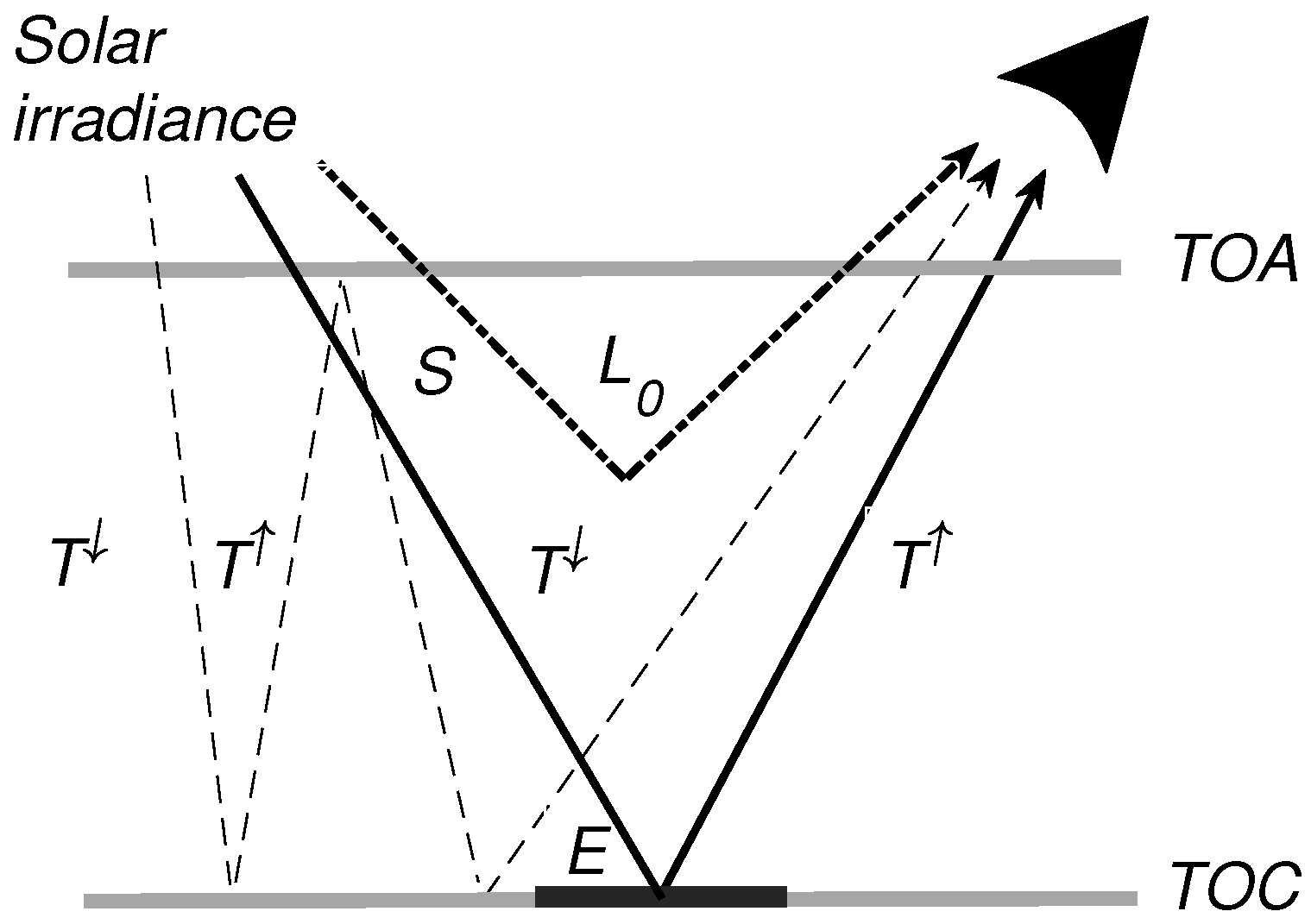
- The scattered light from the atmosphere or path radiance (thick dashed-dotted line).
- The reflected light from the observed target which is transmitted to the sensor (solid line).
- The light coming from multiple reflections between the surface and the atmosphere, not necessarily produced at the observed target, but finally reaching the sensor (thin dashed line).
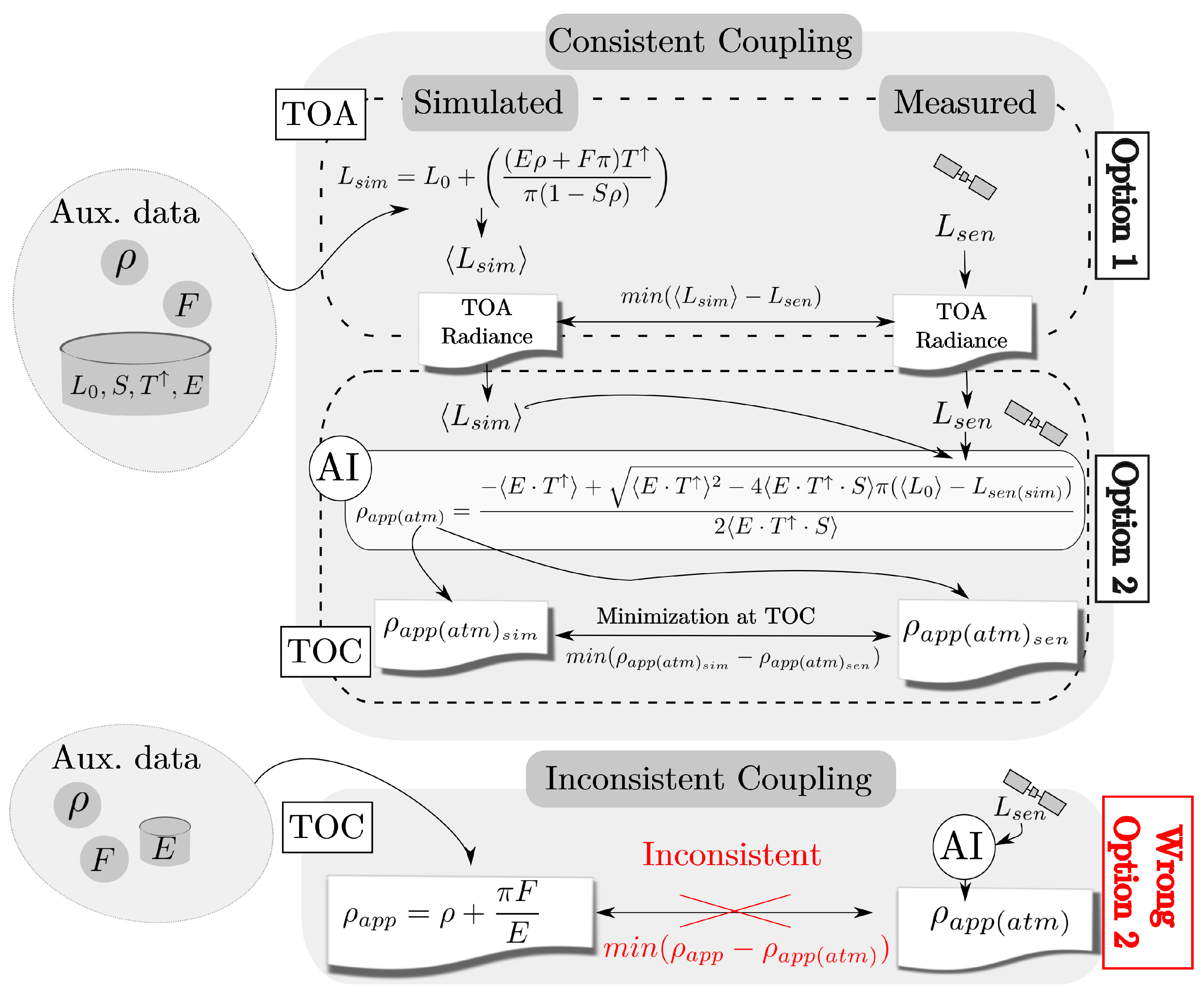
2.2. Coupling Spectral Fitting and Apparent Reflectance
- Option 1: To perform the SF method at TOA level, thereby minimizing the difference between the radiance acquired by the spaceborne instrument and the simulated radiance using Equation (4).
- Option 2: To perform the SF method at TOC level, thereby minimizing the difference between the atmospherically corrected radiance (or apparent reflectance) and the simulated radiance (or apparent reflectance) accounting for the AI procedure.
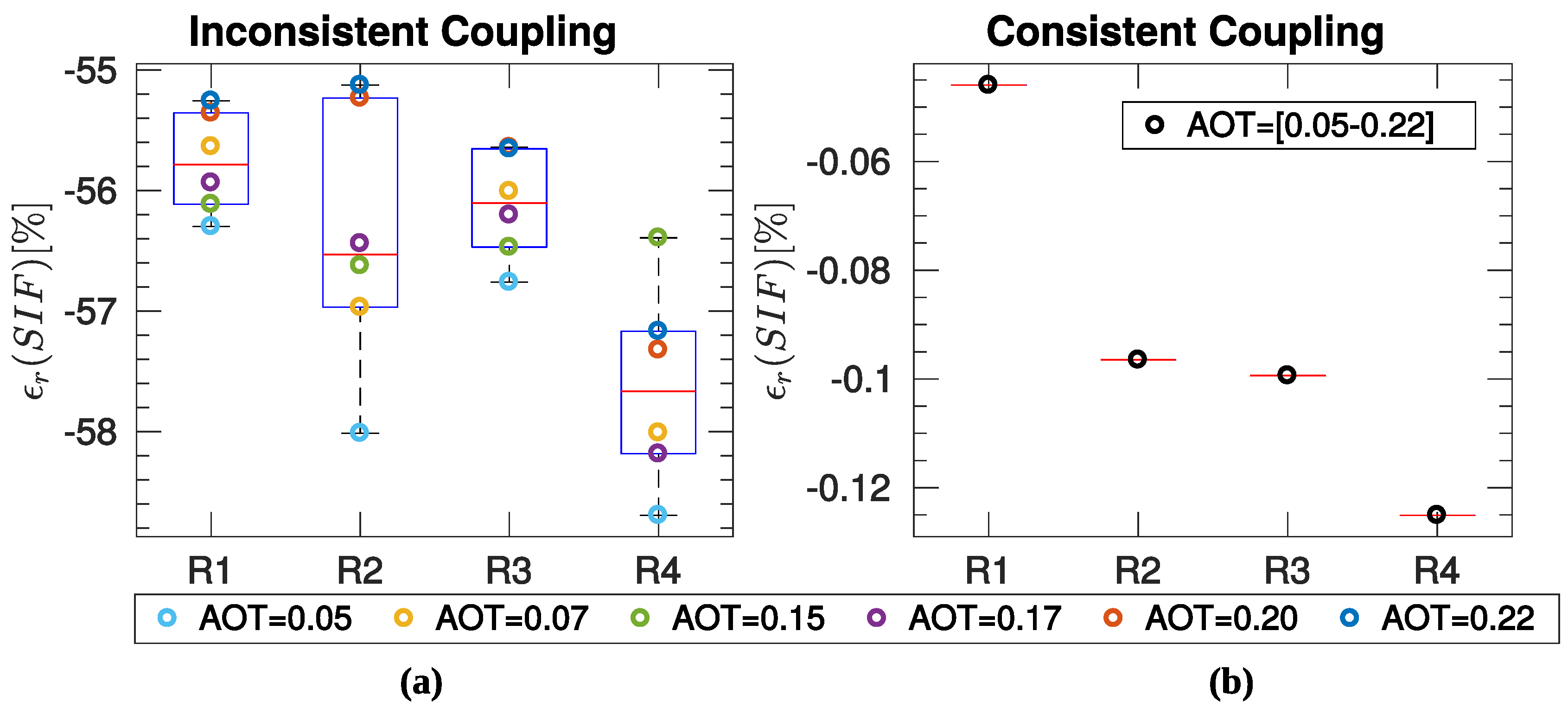
- An inconsistent coupling process, i.e., modelling at TOC as . The inconsistent coupling causes a large relative error between the retrieved and the reference SIF values for all of the minimization wavelength intervals considered (R1–R4). In addition, a slight dependency on the Aerosol Optical Thickness (AOT) can also be observed.
- A consistent coupling between AI and SF as introduced in Figure 5 (Option 2). In this case, all of the SIF retrieved values (i.e., for the different AOT) are overlapping, meaning that when the atmospheric state is perfectly known , the retrieved SIF is completely independent from the AOT value. Consequently, the accuracy of the SF minimization process only depends on the wavelength interval considered.
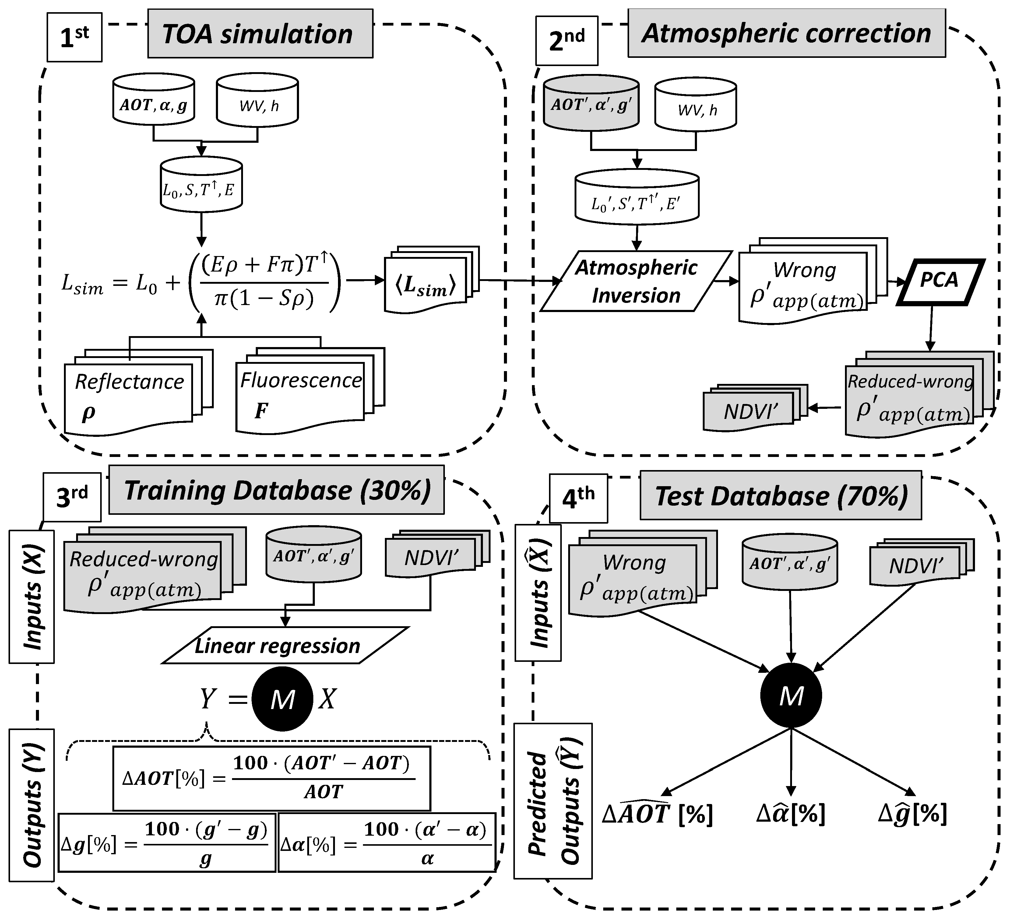
3. Apparent Reflectance Error Analysis and Its Predictive Power
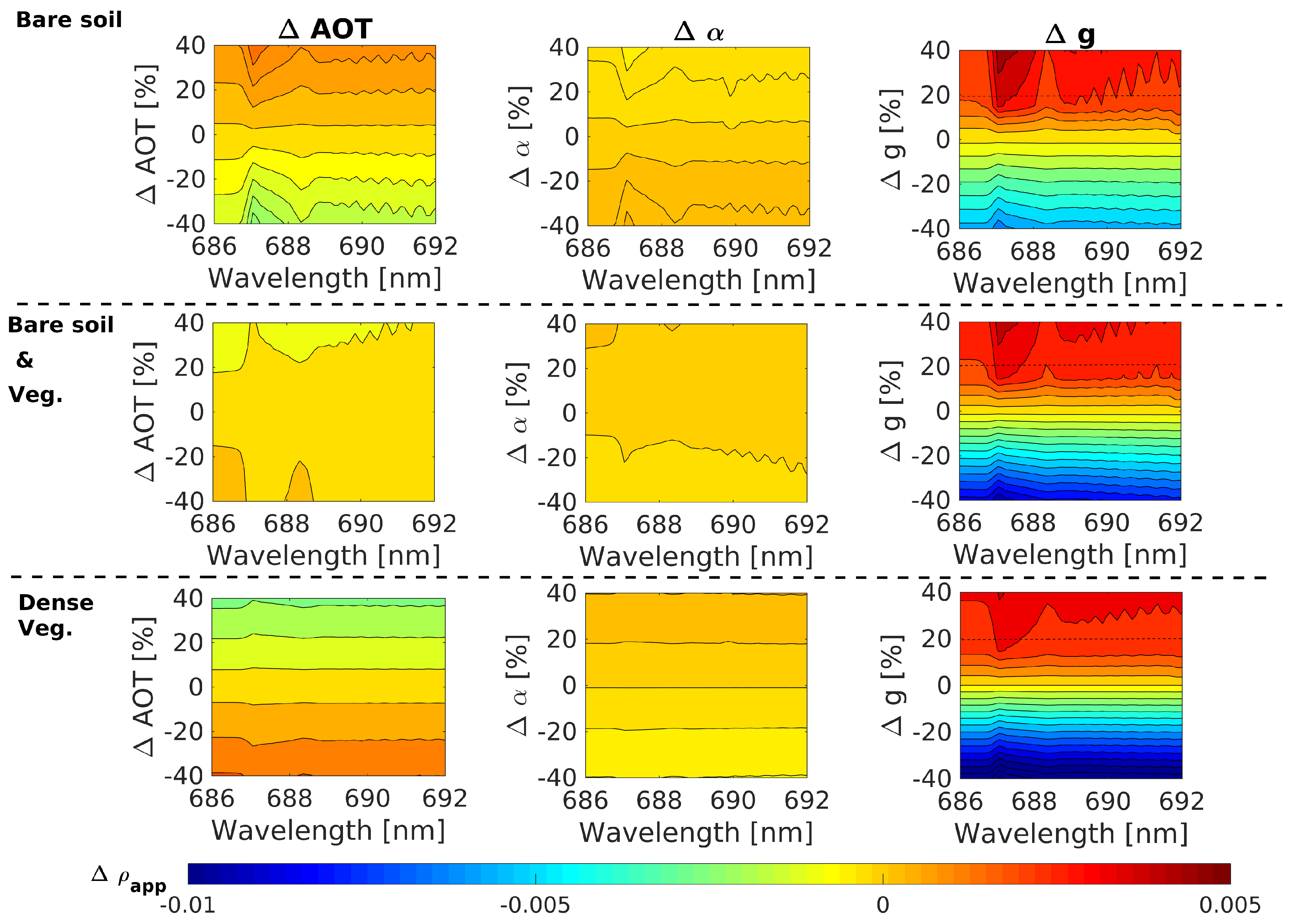
3.1. Spectral Error Analysis on Apparent Reflectance
- the AOT, which is directly related to the total aerosol load in a vertical atmospheric column, becoming a greater aerosol load the higher the AOT value.
- the Angstrom exponent () [35], which accounts for the AOT spectral variation and is associated with the aerosol size, becoming a higher () exponent with a smaller aerosol size.
- the asymmetry parameter (g) of the Henyey–Greenstein (HG) scattering phase function [36], which indicates the anisotropy of the scattering pattern, this parameter being limited to [, 1]. The g parameter takes the value and 1 for a full backward and forward scattering respectively, while taking the value 0 for an isotropic scattering pattern.
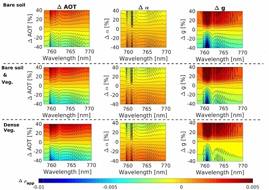
- The over-/under-estimation of the AOT causes an under-/over-estimation of in SIF emitting surfaces, i.e., partially-mixed or dense vegetation, while the opposite effect is observed in non-SIF emitting surfaces, i.e., bare soil.
- Errors in the the Angstrom parameter () hardly lead to errors in . However, the spectral distortion appears to be driven by the underlying surface reflectance, the spectral distortions being more abrupt for the bare soil and the mixed vegetation and bare soil than in a full vegetation spectrum.
- The asymmetry parameter (g) of the HG scattering phase function is clearly the driving parameter that causes the strongest distortion in the . Additionally, the spectral distortions mostly follow a similar spectral pattern regardless of the surface reflectance spectra.
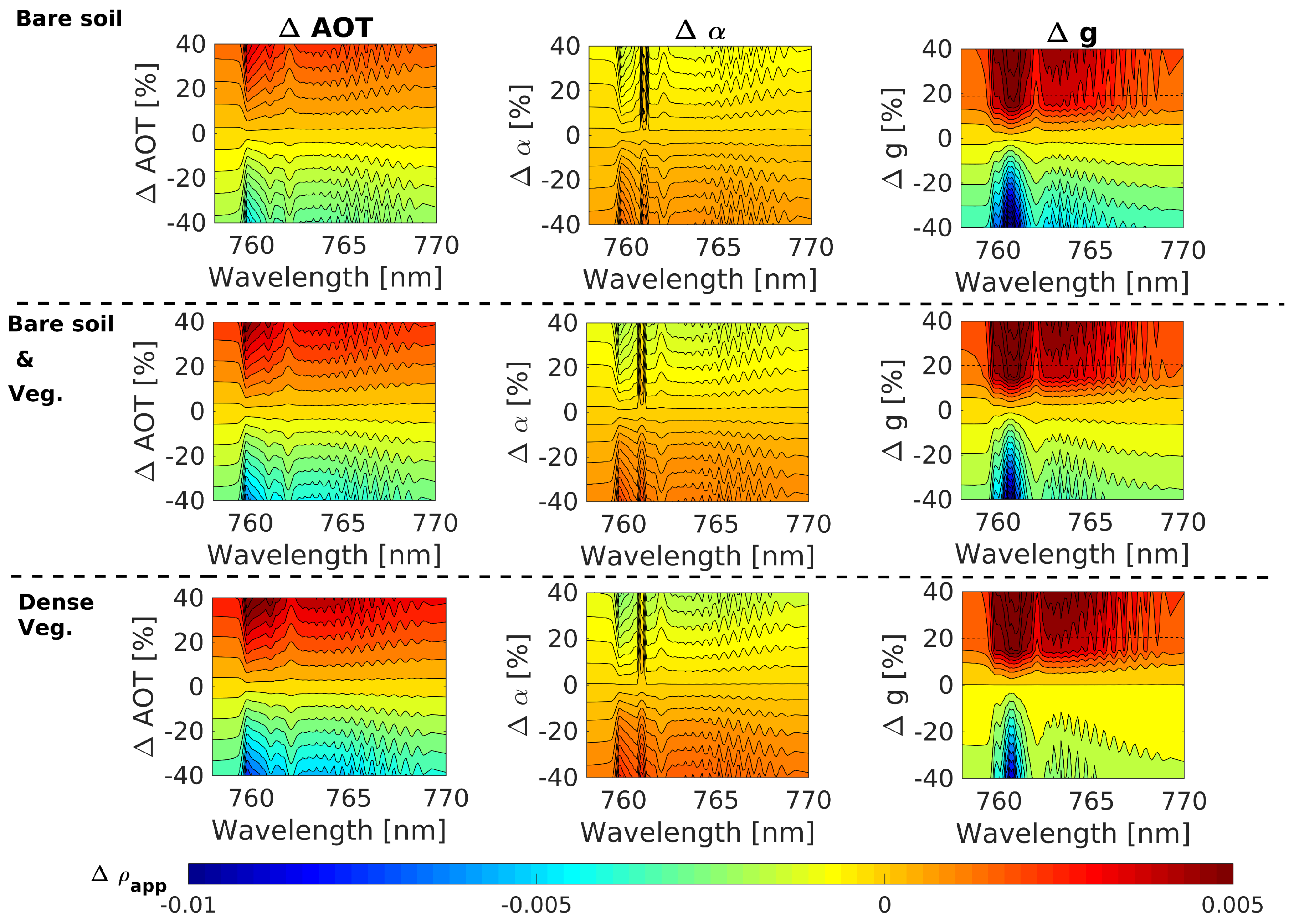
- Spectral distortions in the O2–A caused by each aerosol optical property follow a similar distortion pattern regardless of the surface reflectance and the fluorescence emission. Due to the deepest absorption in the O2–A band, this region seems spectrally more sensitive to aerosol over-/under-estimation.
- Although distortions on produced by changes in the AOT and g, which are the driving parameters, are approximately on the same order of magnitude, the spectral distortion pattern is slightly different.
- As in the O2–B region, the over-/under-estimation of the parameter produces a weaker spectral distortion than those produced by the AOT and the g parameters.
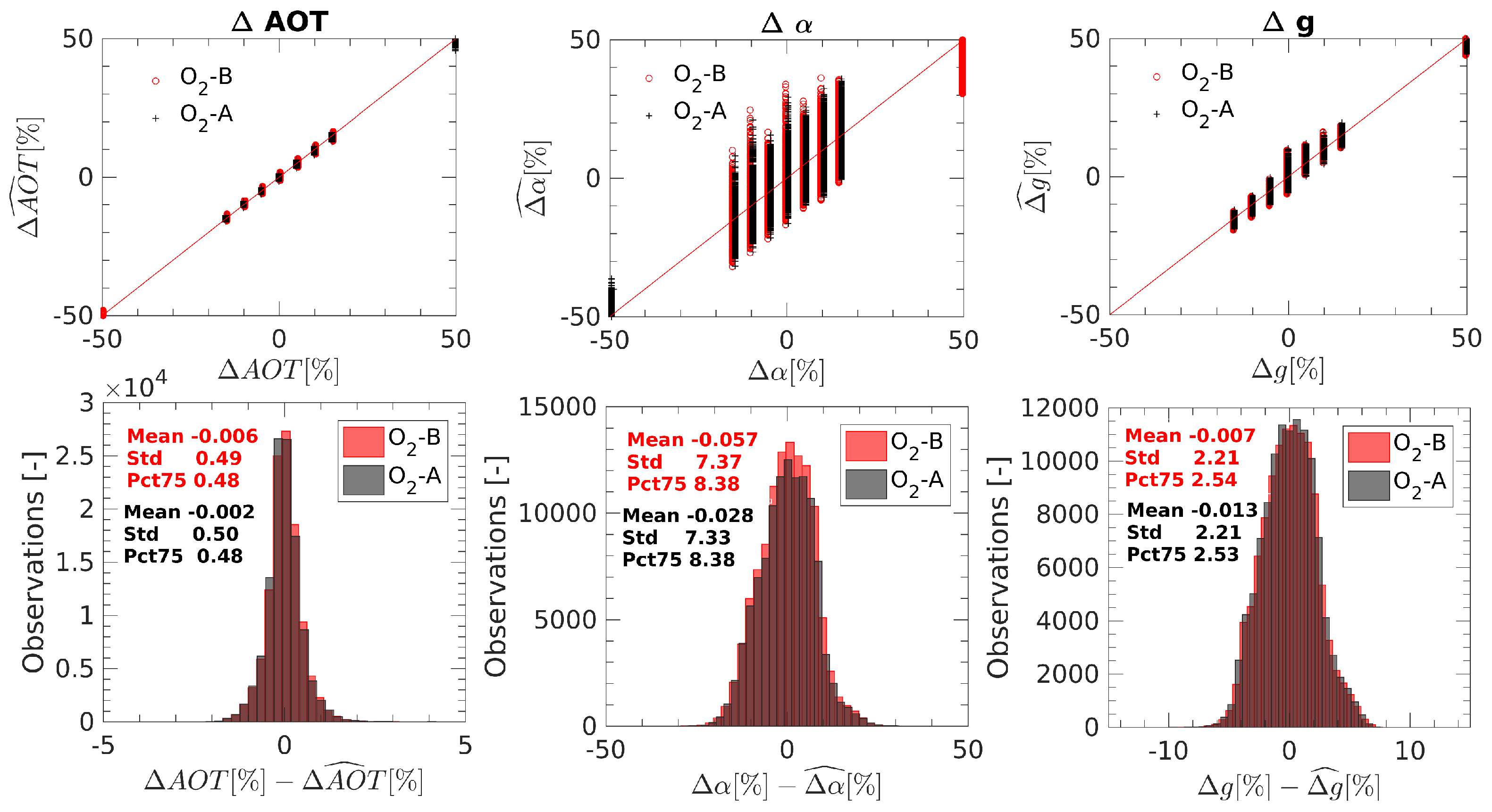
3.2. Spectral Distortions in the Apparent Reflectance as Quality Indicator of the Atmospheric Correction
- to select a medium AOT value to evaluate the aerosols effect but avoiding extreme cases [37];
- to range variations around the and g values of 1.54 and 0.8, respectively, which corresponds to typical values found for continental aerosol types [38];
- to simulate the effect of the surface pressure by including two different altitudes;
- to determine if the different WV content impacts the predictive power of the on the O2–B absorption region.
4. Discussion
4.1. Suitability of the Mathematical Approximations Assumed in the FLEX AI
4.2. Apparent Reflectance Spectral Distortion Analysis and Exploitation
5. Conclusions
Acknowledgments
Author Contributions
Conflicts of Interest
Abbreviations
| AC | Atmospheric Correction |
| AI | Atmospheric Inversion |
| AOT | Aerosol Optical Thickness |
| DB | DataBase |
| FLEX | FLuorescence EXplorer |
| FLORIS | FLuORescence Imaging Spectrometer |
| HG | Henyey–Greenstein |
| HR | High Resolution |
| ISRF | Instrumental Spectral Response Function |
| LAI | Leaf Area Index |
| PCA | Principal Components Analysis |
| SF | Spectral Fitting |
| SIF | Solar-Induced chlorophyll Fluorescence |
| SR | Spectral Resolution |
| SSI | Spectral Sampling Interval |
| TOA | Top Of Atmosphere |
| TOC | Top Of Canopy |
| WV | Water Vapour |
Appendix A

| Band | PRI Band | Chl abs. | O2–B | Red-Edge | O2–A | |||||
|---|---|---|---|---|---|---|---|---|---|---|
| (nm) | 500–600 | 600–677 | 677–686 | 686–697 | 697–740 | 740–755 | 755–759 | 759–762 | 762–769 | 769–780 |
| SR (nm) | 3 | 3 | 0.6 | 0.3 | 2 | 0.7 | 0.7 | 0.3 | 0.3 | 0.7 |
| SI (nm) | 2 | 2 | 0.5 | 0.1 | 0.65 | 0.5 | 0.5 | 0.1 | 0.1 | 0.5 |
Appendix B
| MODTRAN Input Parameter | Value (Units) | |
|---|---|---|
| Atmospheric parameter | Model of atmosphere | Mid Latitude Summer |
| AOT at 550 nm | 0.05 (−) | |
| Angstrom exponent | 0.79 (−) | |
| Henyey–Greenstein asymmetry (g) | 0.8 (−) | |
| Water vapour | 2.4 (g/cm2) | |
| Geometry parameter | Surface elevation | 100 (m) |
| Solar Zenith Angle | 45 (°) | |
| Viewing Zenith Angle | 0 (°) | |
| Relative Azimuth Angle between sun and sensor | 0 (°) | |
| High Spectral Resolution | Spectral Resolution at O2–B | 0.005 (nm) |
| Spectral Resolution at O2–A | 0.006 (nm) | |
| Instrumental Spectral Response | Spectral function | Double sigmoid * |
| Spectral Sampling Interval (SSI) | 0.1 (nm) | |
| Spectral bandwidth () | 0.3 (nm) |
Appendix C
| LAI (−) | Chl (g/cm2) | ||
|---|---|---|---|
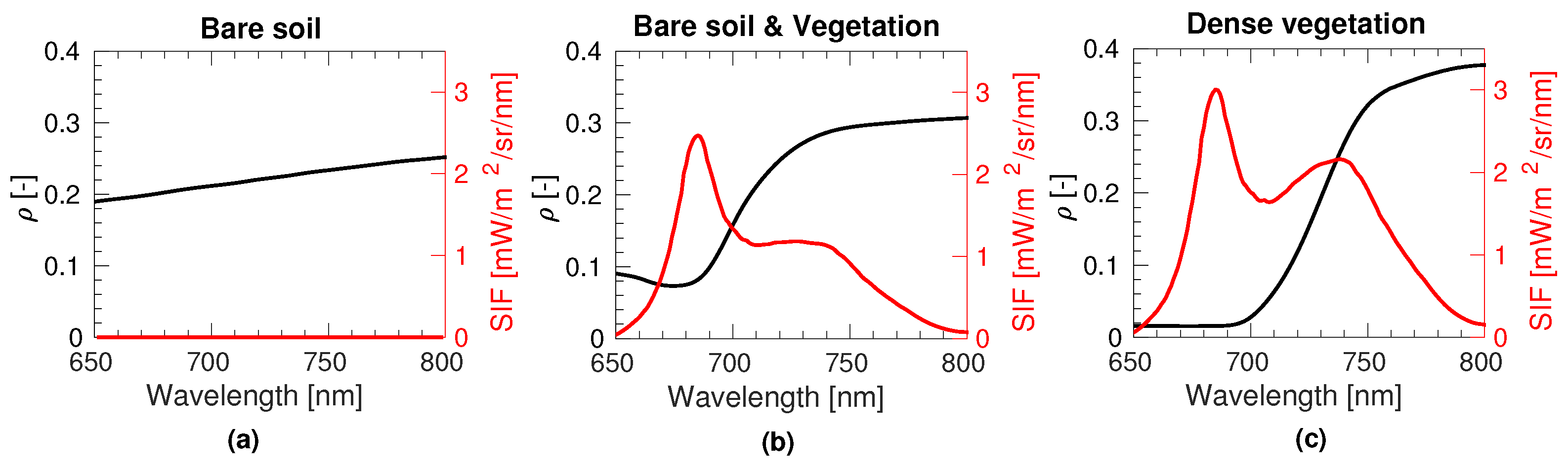
| Bare soil (a) | 0 | 0.47 | |
| Mixed bare soil and dense vegetation | 0.5 | 40 | |
| Mixed bare soil and dense vegetation (b) | 1.5 | 10 | |
| Mixed bare soil and dense vegetation | 2.5 | 40 | |
| Dense vegetation (c) | 4 | 70 |
References
- Porcar-Castell, A.; Tyystjarvi, E.; Atherton, J.; van der Tol, C.; Flexas, J.; Pfundel, E.E.; Moreno, J.; Frankenberg, C.; Berry, J.A. Linking chlorophyll a fluorescence to photosynthesis for remote sensing applications: Mechanisms and challenges. J. Exp. Bot. 2014, 65, 4065–4095. [Google Scholar] [CrossRef]
- Joiner, J.; Yoshida, Y.; Vasilkov, A.P.; Yoshida, Y.; Corp, L.A.; Middleton, E.M. First observations of global and seasonal terrestrial chlorophyll fluorescence from space. Biogeosciences 2011, 8, 637–651. [Google Scholar] [CrossRef]
- Ni, Z.; Liu, Z.; Li, Z.L.; Nerry, F.; Huo, H.; Sun, R.; Yang, P.; Zhang, W. Investigation of Atmospheric Effects on Retrieval of Sun-Induced Fluorescence Using Hyperspectral Imagery. Sensors 2016, 16, 480. [Google Scholar] [CrossRef]
- Joiner, J.; Yoshida, Y.; Vasilkov, A.; Middleton, E.; Campbell, P.; Kuze, A.; Corp, L.A. Filling-in of near-infrared solar lines by terrestrial fluorescence and other geophysical effects: Simulations and space-based observations from SCIAMACHY and GOSAT. Atmos. Meas. Tech. 2012, 5, 809. [Google Scholar] [CrossRef]
- Guanter, L.; Frankenberg, C.; Dudhia, A.; Lewis, P.E.; Gómez-Dans, J.; Kuze, A.; Suto, H.; Grainger, R.G. Retrieval and global assessment of terrestrial chlorophyll fluorescence from GOSAT space measurements. Remote Sens. Environ. 2012, 121, 236–251. [Google Scholar] [CrossRef]
- Khosravi, N. Terrestrial Plant Fluorescence as Seen From Satellite Data. Master’s Thesis, University of Bremen, Bremen, Germany, 2012. [Google Scholar]
- Köhler, P.; Guanter, L.; Joiner, J. A linear method for the retrieval of sun-induced chlorophyll fluorescence from GOME-2 and SCIAMACHY data. Atmos. Meas. Tech. 2015, 8, 2589–2608. [Google Scholar] [CrossRef]
- Köhler, P.; Guanter, L.; Frankenberg, C. Simplified physically based retrieval of sun-induced chlorophyll fluorescence from GOSAT data. IEEE Geosci. Remote Sens. Lett. 2015, 12, 1446–1450. [Google Scholar] [CrossRef]
- Guanter, L.; Alonso, L.; Gómez-Chova, L.; Amorós-López, J.; Vila, J.; Moreno, J. Estimation of solar-induced vegetation fluorescence from space measurements. Geophys. Res. Lett. 2007, 34. [Google Scholar] [CrossRef]
- Damm, A.; Schickling, A.; Schlapfer, D.; Schaepman, M.; Rascher, U. Deriving sun-induced chlorophyll fluorescence from airborne based spectrometer data. In Proceedings of the Hyperspectral 2010 Workshop (SP-683), Frascati, Italy, 17–19 March 2010; pp. 1–7. [Google Scholar]
- Guanter, L.; Alonso, L.; Gómez-Chova, L.; Meroni, M.; Preusker, R.; Fischer, J.; Moreno, J. Developments for vegetation fluorescence retrieval from spaceborne high-resolution spectrometry in the O2–A and O2–B absorption bands. J. Geophys. Res. Atmos. 2010, 115. [Google Scholar] [CrossRef]
- Mazzoni, M.; Falorni, P.; Verhoef, W. High-resolution methods for fluorescence retrieval from space. Opt. Express 2010, 18, 15649–15663. [Google Scholar] [CrossRef]
- Frankenberg, C.; Butz, A.; Toon, G. Disentangling chlorophyll fluorescence from atmospheric scattering effects in O2 A-band spectra of reflected sun-light. Geophys. Res. Lett. 2011, 38. [Google Scholar] [CrossRef]
- Raychaudhuri, B. Solar-induced fluorescence of terrestrial chlorophyll derived from the O2–A band of Hyperion hyperspectral images. Remote Sens. Lett. 2014, 5, 941–950. [Google Scholar] [CrossRef]
- Liu, X.; Liu, L.; Zhang, S.; Zhou, X. New spectral fitting method for full-spectrum solar-induced chlorophyll fluorescence retrieval based on principal components analysis. Remote Sens. 2015, 7, 10626–10645. [Google Scholar] [CrossRef]
- Damm, A.; Guanter, L.; Laurent, V.; Schaepman, M.; Schickling, A.; Rascher, U. FLD-based retrieval of sun-induced chlorophyll fluorescence from medium spectral resolution airborne spectroscopy data. Remote Sens. Environ. 2014, 147, 256–266. [Google Scholar] [CrossRef]
- Cogliati, S.; Verhoef, W.; Kraft, S.; Sabater, N.; Alonso, L.; Vicent, J.; Moreno, J.; Drusch, M.; Colombo, R. Retrieval of sun-induced fluorescence using advanced spectral fitting methods. Remote Sens. Environ. 2015, 169, 344–357. [Google Scholar] [CrossRef]
- Sabater, N.; Alonso, L.; Cogliati, S.; Vicent, J.; Tenjo, C.; Verrelst, J.; Moreno, J. A sun-induced vegetation fluorescence retrieval method from top of atmosphere radiance for the FLEX/Sentinel-3 TanDEM mission. In Proceedings of the 2015 IEEE International Geoscience and Remote Sensing Symposium (IGARSS), Milan, Italy, 26–31 July 2015; pp. 2669–2672. [Google Scholar]
- Guanter, L.; Rossini, M.; Colombo, R.; Meroni, M.; Frankenberg, C.; Lee, J.E.; Joiner, J. Using field spectroscopy to assess the potential of statistical approaches for the retrieval of sun-induced chlorophyll fluorescence from ground and space. Remote Sens. Environ. 2013, 133, 52–61. [Google Scholar] [CrossRef]
- Joiner, J.; Guanter, L.; Lindstrot, R.; Voigt, M.; Vasilkov, A.; Middleton, E.; Huemmrich, K.; Yoshida, Y.; Frankenberg, C. Global monitoring of terrestrial chlorophyll fluorescence from moderate spectral resolution near-infrared satellite measurements: Methodology, simulations, and application to GOME-2. Atmos. Meas. Tech. 2013, 6, 2803–2823. [Google Scholar] [CrossRef]
- Joiner, J.; Yoshida, Y.; Guanter, L.; Middleton, E.M. New methods for retrieval of chlorophyll red fluorescence from hyper-spectral satellite instruments: Simulations and application to GOME-2 and SCIAMACHY. Atmos. Meas. Tech. Discuss. 2016, 9, 1–41. [Google Scholar] [CrossRef]
- European Space Agency (ESA). Report for Mission Selection: FLEX; Technical Report, (SP-1330/2); European Space Agency: Noordwijk, The Netherlands, 2015. [Google Scholar]
- Frankenberg, C.; O’Dell, C.; Guanter, L.; McDuffie, J. Remote sensing of near-infrared chlorophyll fluorescence from space in scattering atmospheres: Implications for its retrieval and interferences with atmospheric CO2 retrievals. Atmos. Meas. Tech. 2012, 5, 2081–2094. [Google Scholar] [CrossRef]
- Meroni, M.; Busetto, L.; Colombo, R.; Guanter, L.; Moreno, J.; Verhoef, W. Performance of spectral fitting methods for vegetation fluorescence quantification. Remote Sens. Environ. 2010, 114, 363–374. [Google Scholar] [CrossRef]
- Tol, C.; Verhoef, W.; Timmermans, J.; Verhoef, A.; Su, Z. An integrated model of soil-canopy spectral radiances, photosynthesis, fluorescence, temperature and energy balance. Biogeosciences 2009, 6, 3109–3129. [Google Scholar]
- Berk, A.; Anderson, G.P.; Acharya, P.K.; Bernstein, L.S.; Muratov, L.; Lee, J.; Fox, M.; Adler-Golden, S.M.; Chetwynd, J.H.; Hoke, M.L.; et al. MODTRAN 5: A reformulated atmospheric band model with auxiliary species and practical multiple scattering options. Proc. SPIE 2005, 5655, 88–95. [Google Scholar]
- Vermote, E.; Tanré, D.; Deuzé, J.; Herman, J.; Kotchenova, S. Second Simulation of a Satellite Signal in the Solar Spectrum-Vector (6SV), User Guide Version 3; Technical Report; Department of Geography-University of Maryland: College Park, MD, USA; Laboratoire d’Optique Atmopherique-Université des Sciences et Technologies de Lille: Villeneuve-d’Ascq, France; European Centre for Medium Range Weather Forecast (ECWMF): Reading, UK, 2006. [Google Scholar]
- Moreno, J.; Alonso, L.; Vicent, J. Technical Note on FLORIS Reference TOA Radiance; Technical Report; LEO Group, Image Processing Laboratory (IPL), University of Valencia: Valencia, Spain, 2012. [Google Scholar]
- Vermote, E.F.; Tanré, D.; Deuze, J.L.; Herman, M.; Morcette, J.J. Second simulation of the satellite signal in the solar spectrum, 6S: An overview. IEEE Trans. Geosci. Remote Sens. 1997, 35, 675–686. [Google Scholar] [CrossRef]
- Verhoef, W.; Van del Tol, C.; Middleton, E.M. Vegetation canopy fluorescence and reflectance retrieval by model inversion using optimization. In Proceedings of the 5th International ESA Workshop on Remote Sensing of Vegetation Fluorescence, Paris, France, 22–24 April 2014. [Google Scholar]
- Vicent, J.; Alonso, L.; Sabater, N.; Miesch, C.; Kraft, S.; Moreno, J. Propagation of spectral characterization errors of imaging spectrometers at level-1 and its correction within a level-2 recalibration scheme. Proc. SPIE 2015, 9611, 96110T. [Google Scholar]
- Guanter, L.; Del Carmen González-Sanpedro, M.; Moreno, J. A method for the atmospheric correction of ENVISAT/MERIS data over land targets. Int. J. Remote Sens. 2007, 28, 709–728. [Google Scholar] [CrossRef]
- Vermote, E.F.; El Saleous, N.Z.; Justice, C.O. Atmospheric correction of MODIS data in the visible to middle infrared: First results. Remote Sens. Environ. 2002, 83, 97–111. [Google Scholar] [CrossRef]
- Cooley, T.; Anderson, G.; Felde, G.; Hoke, M.; Ratkowski, A.; Chetwynd, J.; Gardner, J.; Adler-Golden, S.; Matthew, M.; Berk, A.; et al. FLAASH, a MODTRAN4-based atmospheric correction algorithm, its application and validation. In Proceedings of the 2002 IEEE International Geoscience and Remote Sensing Symposium (IGARSS’02), Toronto, ON, Canada, 24–28 June 2002; Volume 3, pp. 1414–1418. [Google Scholar]
- Ångström, A. On the atmospheric transmission of sun radiation and on dust in the air. Geogr. Ann. 1929, 11, 156–166. [Google Scholar] [CrossRef]
- Henyey, L.G.; Greenstein, J.L. Diffuse radiation in the galaxy. Astrophys. J. 1941, 93, 70–83. [Google Scholar] [CrossRef]
- Dubovik, O.; Holben, B.; Eck, T.F.; Smirnov, A.; Kaufman, Y.J.; King, M.D.; Tanré, D.; Slutsker, I. Variability of absorption and optical properties of key aerosol types observed in worldwide locations. J. Atmos. Sci. 2002, 59, 590–608. [Google Scholar] [CrossRef]
- Hess, M.; Koepke, P.; Schult, I. Optical properties of aerosols and clouds: The software package OPAC. Bull. Am. Meteorol. Soc. 1998, 79, 831–844. [Google Scholar] [CrossRef]
- Daumard, F.; Goulas, Y.; Ounis, A.; Pedrós, R.; Moya, I. Measurement and correction of atmospheric effects at different altitudes for remote sensing of sun-induced fluorescence in oxygen absorption bands. IEEE Trans. Geosci. Remote Sens. 2015, 53, 5180–5196. [Google Scholar] [CrossRef]
- Vicent, J.; Alonso, L.; Cogliati, S.; Damm, A.; Pinto, F.; Sabater, N.; Rasher, U.; Verrelst, J.; Moreno, J. HyPlant Airborne Data Processing in the Context of the HYFLEX 2012/13 Field Campaign for the Retrieval of Sun-Induced Fluorescence Emission. In Proceedings of the 5th International ESA Workshop on Remote Sensing of Vegetation Fluorescence, Paris, France, 22–24 April 2014. [Google Scholar]
- Verrelst, J.; Sabater, N.; Rivera, J.P.; Muñoz-Marí, J.; Vicent, J.; Camps-Valls, G.; Moreno, J. Emulation of Leaf, Canopy and Atmosphere Radiative Transfer Models for Fast Global Sensitivity Analysis. Remote Sens. 2016, 8, 673. [Google Scholar] [CrossRef]
- Vicent, J.; Sabater, N.; Verrelst, J.; Alonso, L.; Moreno, J. Assessment of approximations in aerosol optical properties and vertical distribution into FLEX atmospherically-corrected surface reflectance and retrieved Sun-induced fluorescence. Remote Sens. 2017. submitted. [Google Scholar]
- Vicent, J.; Sabater, N.; Tenjo, C.; Acarreta, J.R.; Manzano, M.; Rivera, J.P.; Jurado, P.; Franco, R.; Alonso, L.; Verrelst, J.; et al. FLEX end-to-end mission performance simulator. IEEE Trans. Geosci. Remote Sens. 2016, 54, 4215–4223. [Google Scholar] [CrossRef]


© 2017 by the authors. Licensee MDPI, Basel, Switzerland. This article is an open access article distributed under the terms and conditions of the Creative Commons Attribution (CC BY) license (http://creativecommons.org/licenses/by/4.0/).
Share and Cite
Sabater, N.; Vicent, J.; Alonso, L.; Cogliati, S.; Verrelst, J.; Moreno, J. Impact of Atmospheric Inversion Effects on Solar-Induced Chlorophyll Fluorescence: Exploitation of the Apparent Reflectance as a Quality Indicator. Remote Sens. 2017, 9, 622. https://doi.org/10.3390/rs9060622
Sabater N, Vicent J, Alonso L, Cogliati S, Verrelst J, Moreno J. Impact of Atmospheric Inversion Effects on Solar-Induced Chlorophyll Fluorescence: Exploitation of the Apparent Reflectance as a Quality Indicator. Remote Sensing. 2017; 9(6):622. https://doi.org/10.3390/rs9060622
Chicago/Turabian StyleSabater, Neus, Jorge Vicent, Luis Alonso, Sergio Cogliati, Jochem Verrelst, and José Moreno. 2017. "Impact of Atmospheric Inversion Effects on Solar-Induced Chlorophyll Fluorescence: Exploitation of the Apparent Reflectance as a Quality Indicator" Remote Sensing 9, no. 6: 622. https://doi.org/10.3390/rs9060622
APA StyleSabater, N., Vicent, J., Alonso, L., Cogliati, S., Verrelst, J., & Moreno, J. (2017). Impact of Atmospheric Inversion Effects on Solar-Induced Chlorophyll Fluorescence: Exploitation of the Apparent Reflectance as a Quality Indicator. Remote Sensing, 9(6), 622. https://doi.org/10.3390/rs9060622