
The Application of ALOS/PALSAR InSAR to Measure Subsurface Penetration Depths in Deserts


Abstract
:
1. Introduction
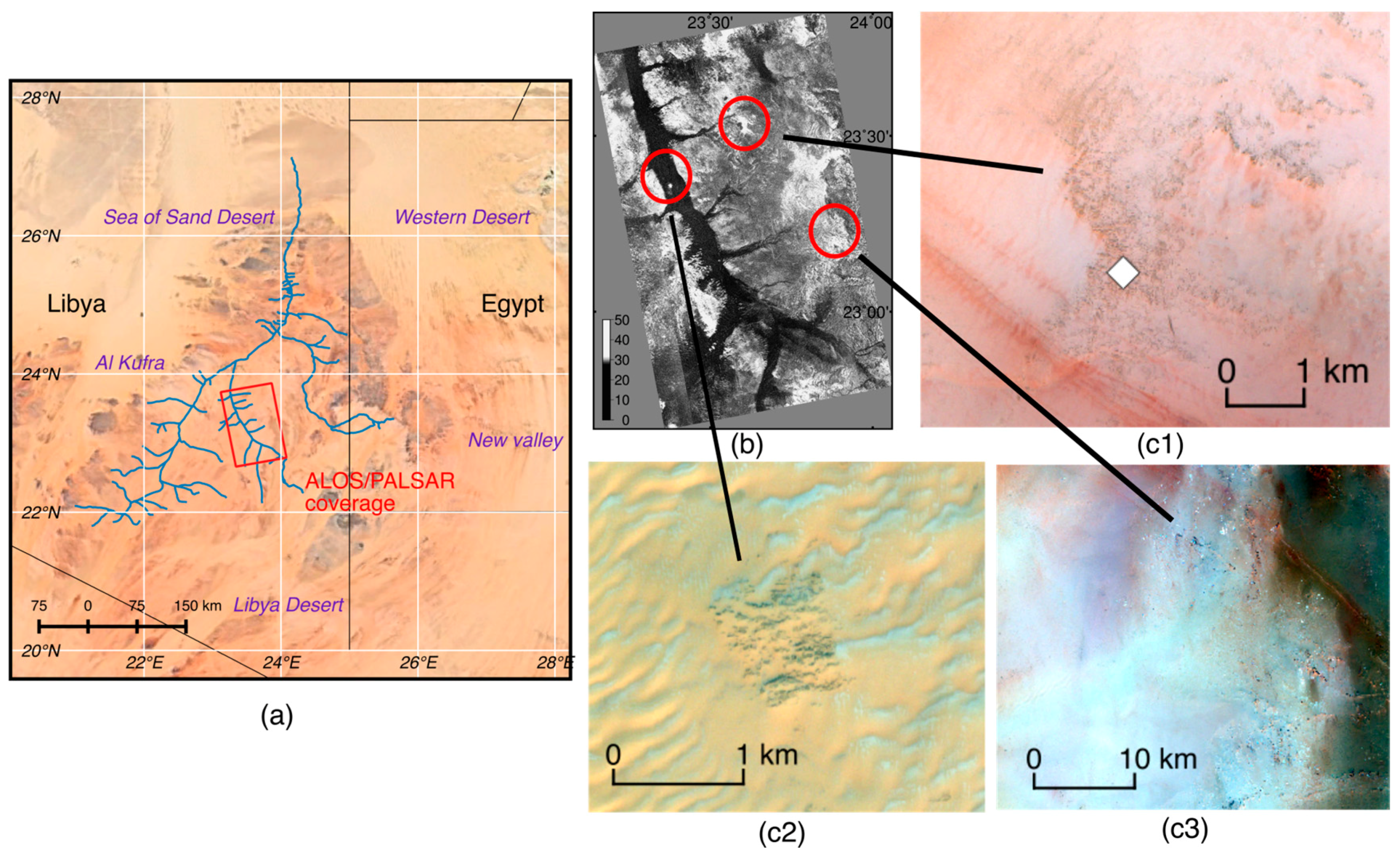
2. Study Site
3. Data and Methods
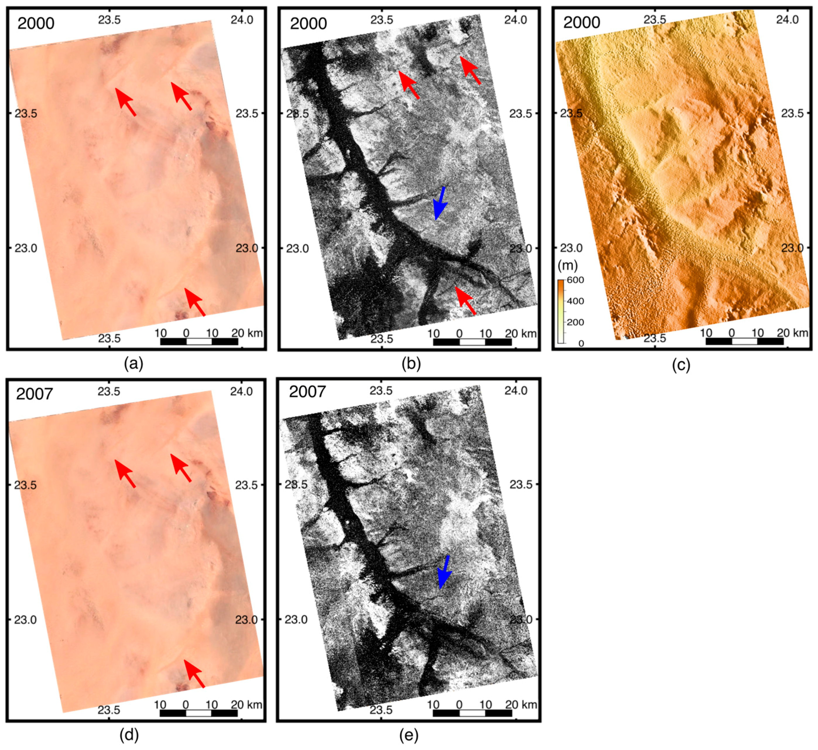
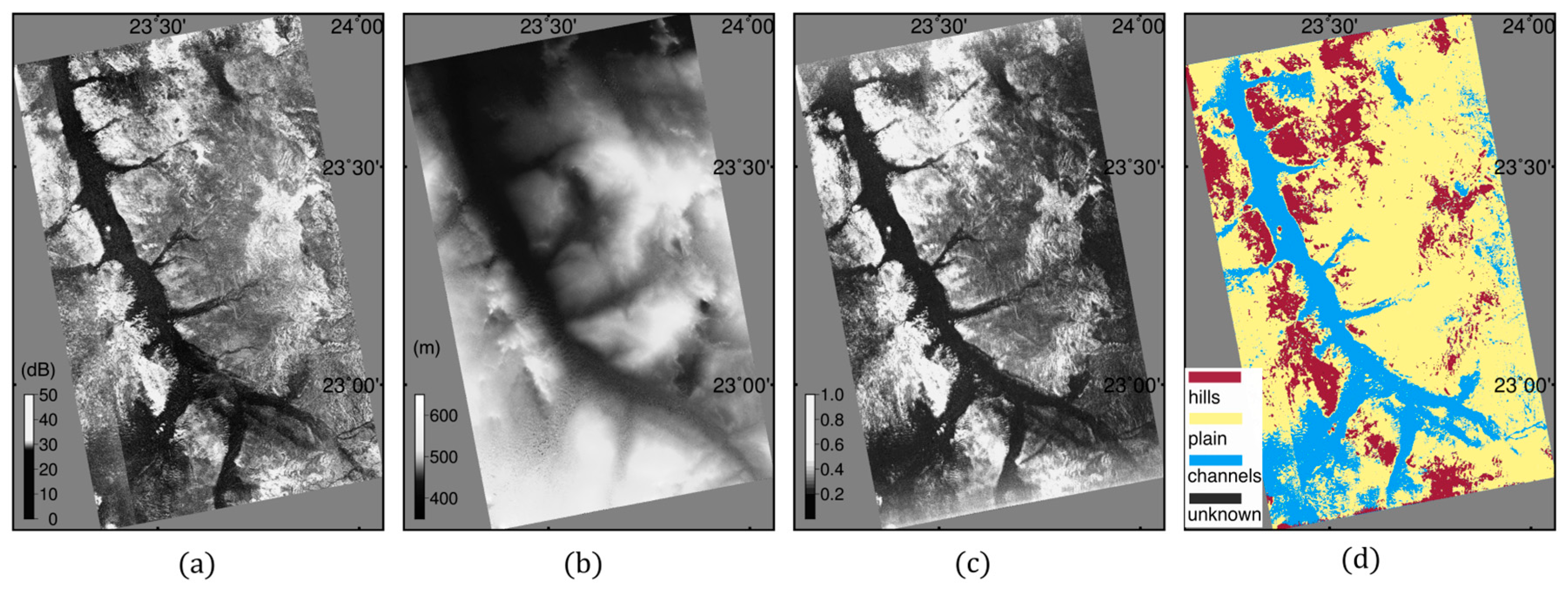
3.1. Comparison of Image Surface Morphology
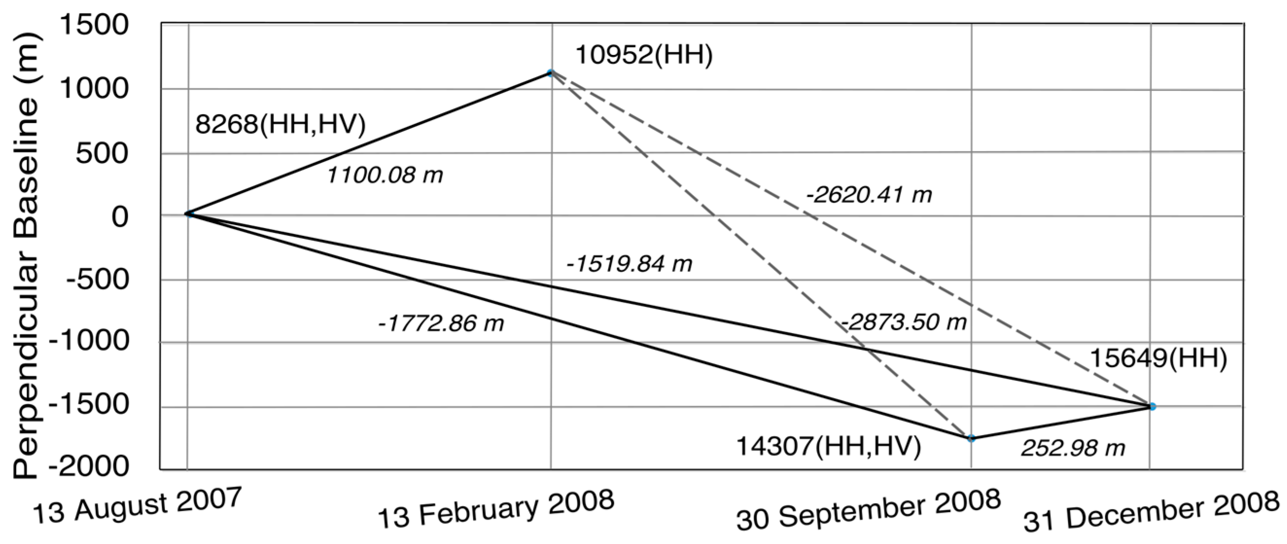
3.2. SAR Interferometry
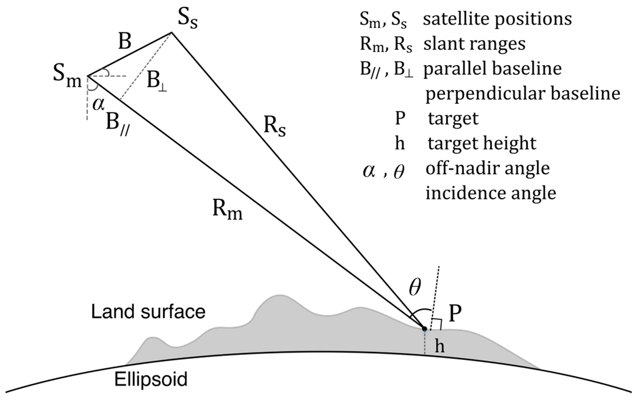
3.2.1. Interferometic Phase Formation
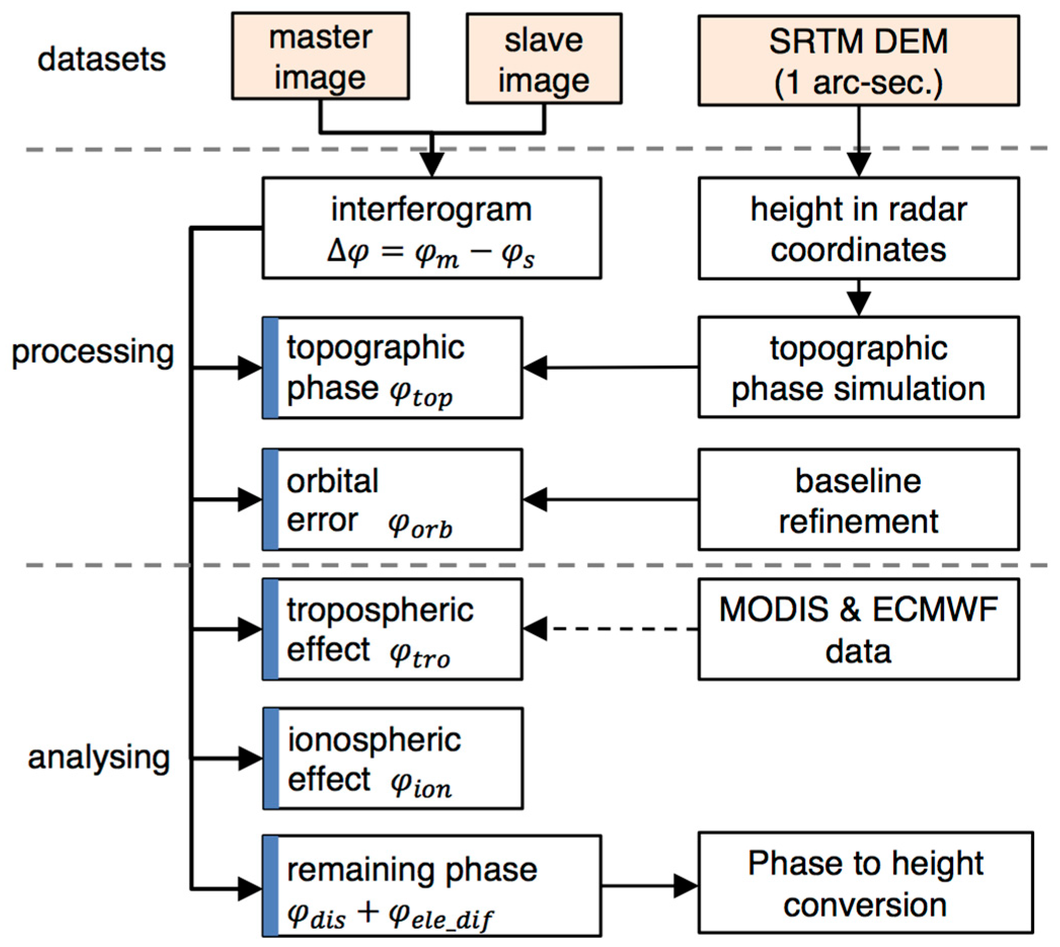
3.2.2. Removal of Topographic and Orbital Phase
3.2.3. Analysis of Remaining Phase Components
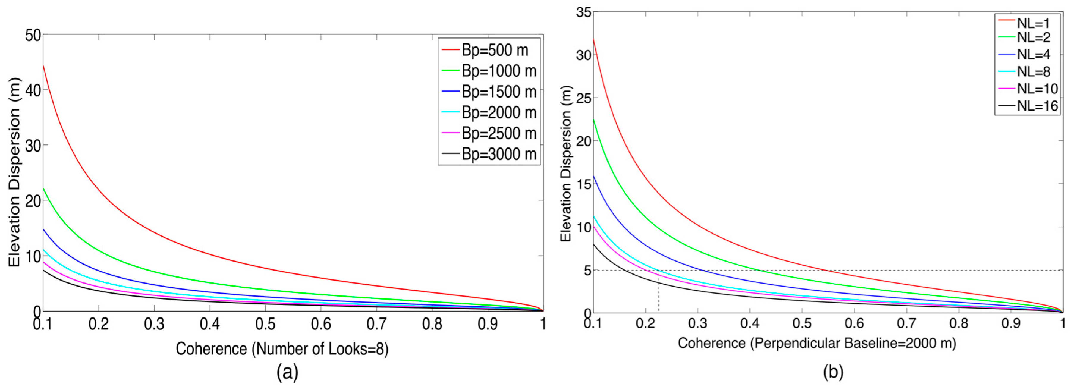
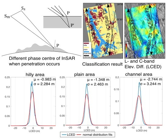
3.3. Estimation of Penetration Depth
3.4. Validation of the Penetration Depth
4. Results
4.1. Comparison of Image Surface Morphology
4.2. SAR Interferometry
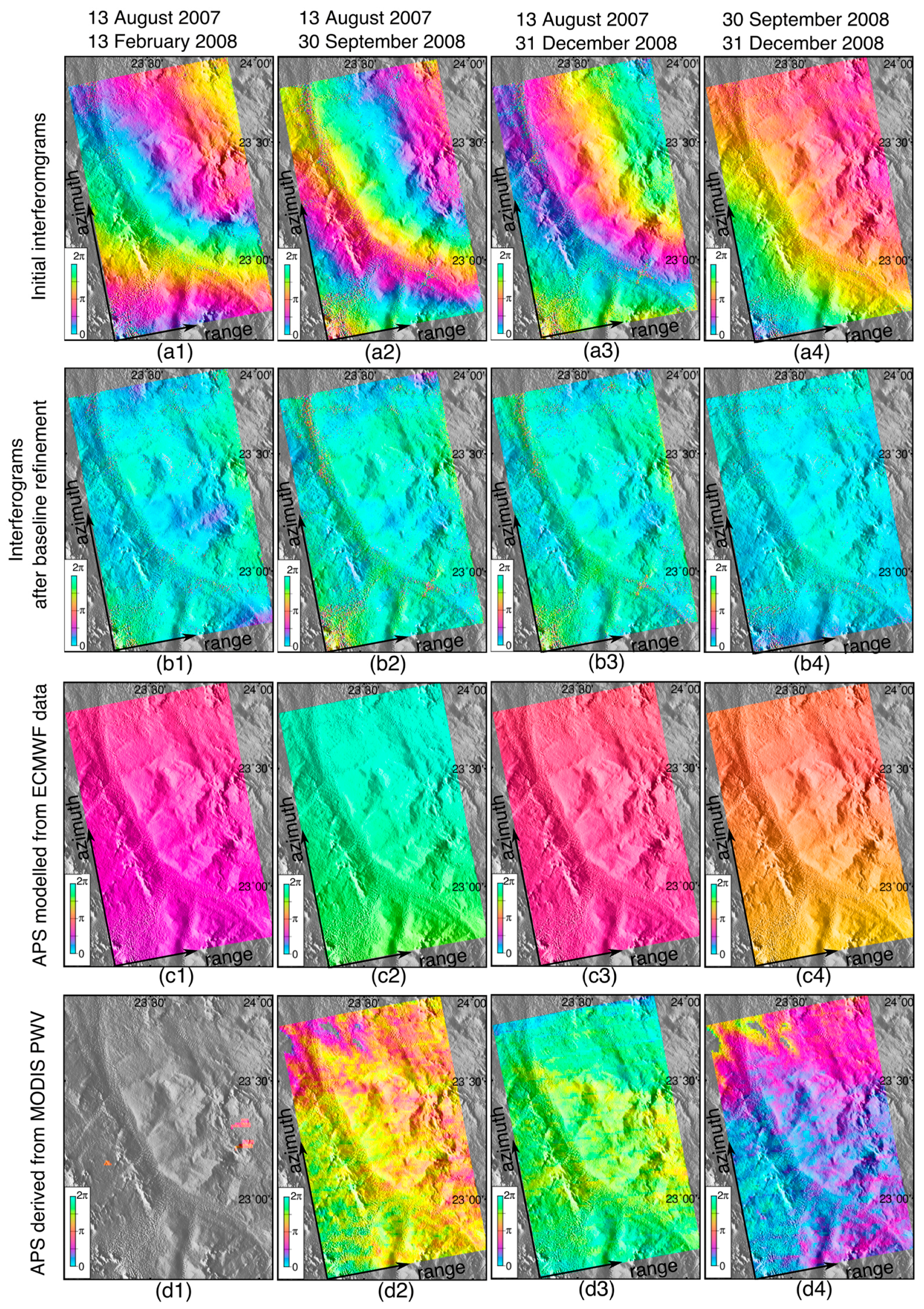
4.2.1. Interferometic Phase Formation
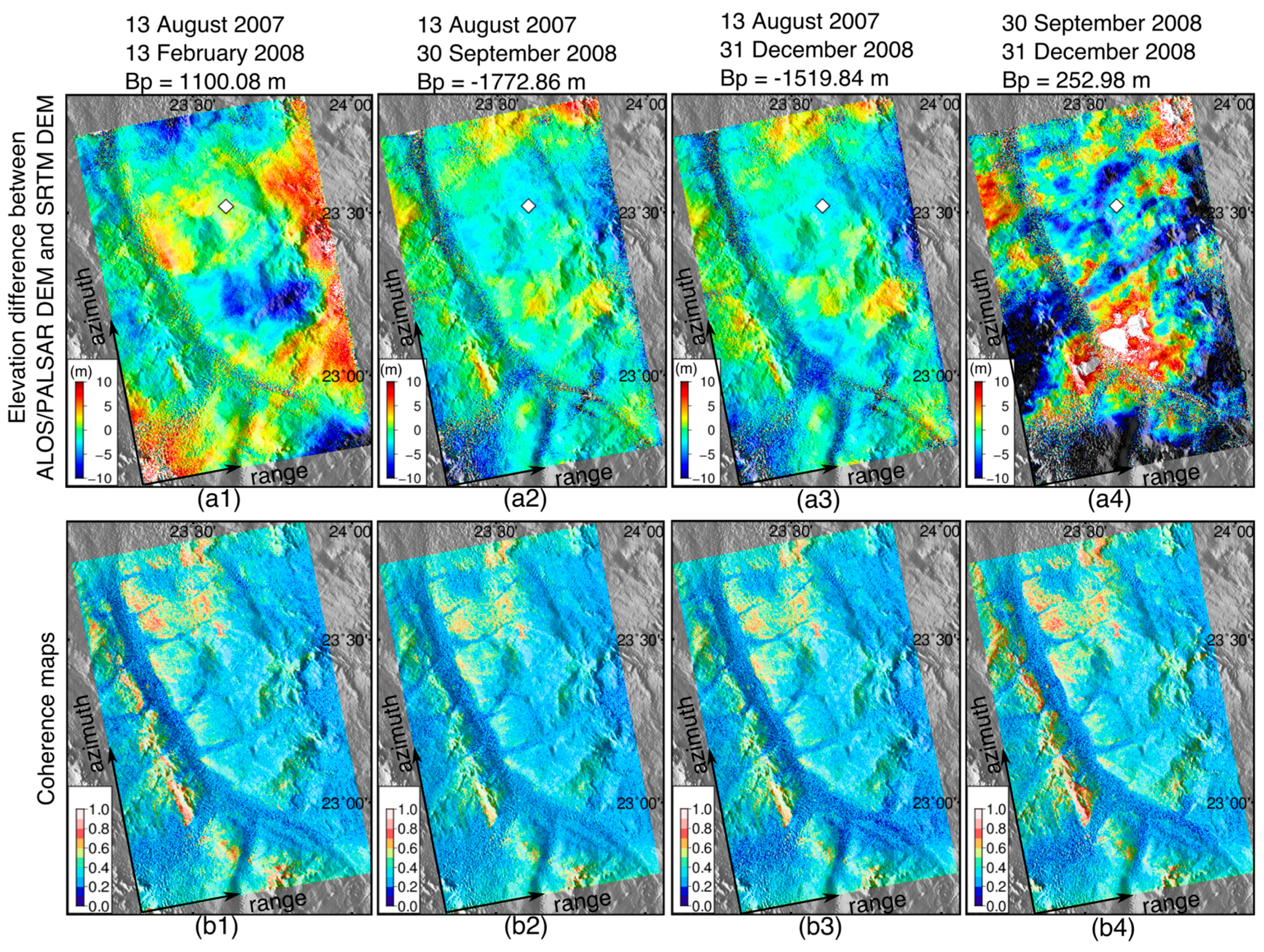
4.2.2. Removal of Topographic and Orbital Phase
4.2.3. Analysis of Remaining Phase Components
4.3. Estimation of Penetration Depth
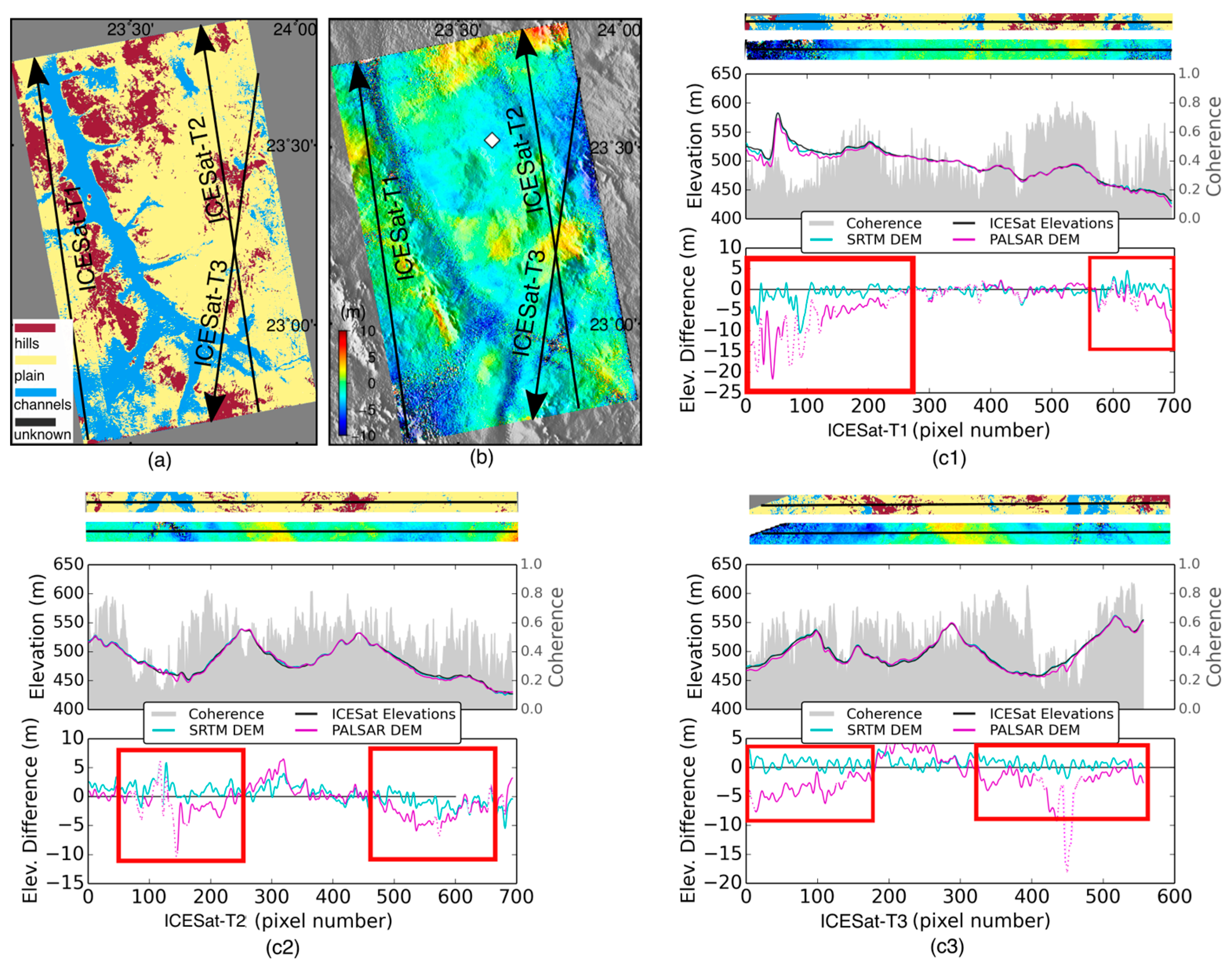
4.4. Validation of the Penetration Depth by ICESat/GLA14
5. Discussion
6. Conclusions
Acknowledgments
Author Contributions
Conflicts of Interest
References
- Elachi, C.; Granger, J. Spaceborne imaging radars probe ‘in depth’: New spaceborne radar sensors allow all-weather, day or night, high-resolution imaging of the earth’s land and ocean surfaces. IEEE Spectr. 1982, 19, 24–29. [Google Scholar] [CrossRef]
- McCauley, J.F.; Schaber, G.G.; Breed, C.S.; Grolier, M.J.; Haynes, C.V.; Issawi, B.; Elachi, C.; Blom, R. Subsurface valleys and geoarcheology of the eastern Sahara revealed by shuttle radar. Science 1982, 218, 1004–1020. [Google Scholar] [CrossRef] [PubMed]
- Roth, L.; Elachi, C. Coherent electromagnetic losses by scattering from volume inhomogeneities. IEEE Trans. Antennas Propag. 1975, 23, 674–675. [Google Scholar] [CrossRef]
- Schaber, G.G.; McCauley, J.F.; Breed, C.S. The use of multifrequency and polarimetric SIR-C/X-SAR data in geologic studies of Bir Safsaf, Egpyt. Remote Sens. Environ. 1997, 59, 337–363. [Google Scholar] [CrossRef]
- Robinson, C.A.; El-Baz, F.; Al-Saud, T.S.M.; Jeon, S.B. Use of radar data to delineate paleodrainage leading to the Kufra Oasis in the eastern Sahara. J. Afr. Earth Sci. 2006, 44, 229–240. [Google Scholar] [CrossRef]
- El-Baz, F.; Maingue, M.; Robinson, C. Fluvio-aeolian dynamics in the north-eastern Sahara: The relationship between fluvial/aeolian systems and ground-water concentration. J. Arid Environ. 2000, 44, 173–183. [Google Scholar] [CrossRef]
- Robinson, C.; El-Baz, F.; Ozdogan, M.; Ledwith, M.; Blanco, D.; Oakley, S.; Inzana, J. Use of radar data to delineate palaeodrainage flow directions in the Selima Sand Sheet, eastern Sahara. Photogramm. Eng. Remote Sens. 2000, 66, 745–753. [Google Scholar]
- Guo, H.; Liu, H.; Wang, X.; Shao, Y.; Sun, Y. Subsurface old drainage detection and paleoenvironment analysis using spaceborne radar images in Alxa Plateau. Sci. China Ser. D Earth Sci. 2000, 43, 439–448. [Google Scholar] [CrossRef]
- Grandjean, G.; Paillou, P.; Baghdadi, N.; Heggy, E.; August, T.; Lasne, Y. Surface and subsurface structural mapping using low frequency radar: A synthesis of the Mauritanian and Egyptian experiments. J. Afr. Earth Sci. 2006, 44, 220–228. [Google Scholar] [CrossRef]
- Paillou, P.; Schuster, M.; Tooth, S.; Farr, T.; Rosenqvist, A.; Lopez, S.; Malezieux, J.M. Mapping of a major paleodrainage system in eastern Libya using orbital imaging radar: The Kufrah River. Earth Planet. Sci. Lett. 2009, 277, 327–333. [Google Scholar] [CrossRef]
- Paillou, P.; Lopez, S.; Farr, T.; Rosenqvist, A. Mapping subsurface geology in Sahara using L- and SAR: First results from the ALOS/PALSAR imaging radar. IEEE J. Sel. Top. Appl. Earth Obs. Remote Sens. 2010, 3, 632–636. [Google Scholar] [CrossRef]
- Sternberg, T.; Paillou, P. Mapping potential shallow groundwater in the Gobi desert using remote sensing: Lake Ulaan Nuur. J. Arid Environ. 2015, 118, 21–27. [Google Scholar] [CrossRef]
- Grenier, C.; Paillou, P.; Maugis, P. Assessment of Holocene surface hydrological connections for the Ounianga lake catchment zone (Chad). C. R. Geosci. 2009, 341, 770–782. [Google Scholar] [CrossRef]
- Jiao, J.J.; Zhang, X.; Wang, X. Satellite-based estimates of groundwater depletion in the Badain Jaran Desert, China. Sci. Rep. 2015, 5, 1–5. [Google Scholar] [CrossRef] [PubMed]
- Ghoneim, E.; El-Baz, F. The application of radar topographic data to mapping of a mega- paleodrainage in the eastern Sahara. J. Arid Environ. 2007, 69, 658–675. [Google Scholar] [CrossRef]
- Dall, J. InSAR elevation bias caused by penetration into uniform volumes. IEEE Trans. Geosci. Remote Sens. 2007, 45, 2319–2324. [Google Scholar] [CrossRef]
- Wang, R.; Hu, C.; Zeng, T.; Long, T.; Yuan, K. Subsurface Height Measurement Using InSAR Technique in Sand-Covered Arid Areas. In Proceedings of the IEEE International Geoscience Remote Sensing Symposium, Québec, QC, Canada, 13–18 July 2014; pp. 422–424. [Google Scholar]
- Elsherbini, A.; Sarabandi, K. Mapping of sand layer thickness in deserts using SAR interferometry. IEEE Trans. Geosci. Remote Sens. 2010, 48, 3550–3559. [Google Scholar] [CrossRef]
- Grandjean, G.; Paillou, P.; Dubois-Fernandez, P.; August-Bernex, T.; Baghdadi, N.N.; Achache, J. Subsurface structures detection by combining L-band polarimetric SAR and GPR data: Example of the Pyla Dune (France). IEEE Trans. Geosci. Remote Sens. 2001, 39, 1245–1258. [Google Scholar] [CrossRef]
- Lasne, Y.; Paillou, P.; August-Bernex, T.; Ruffié, G.; Grandjean, G. A phase signature for detecting wet subsurface structures using polarimetric L-band SAR. IEEE Trans. Geosci. Remote Sens. 2004, 42, 1683–1694. [Google Scholar] [CrossRef]
- NASA. U.S. Releases Enhanced Shuttle Land Elevation Data. Available online: https://www.jpl.nasa.gov/news/news.php?release=2014-321 (accessed on 16 June 2017).
- Gruber, A.; Wessel, B.; Huber, M.; Roth, A. Operational TanDEM-X DEM calibration and first validation results. ISPRS J. Photogramm. Remote Sens. 2012, 73, 39–49. [Google Scholar] [CrossRef]
- Rosenqvist, A.; Shimada, M.; Ito, N.; Watanabe, M. ALOS PALSAR: A Pathfinder Mission for Global-scale Monitoring of the Environment. IEEE Trans. Geosci. Remote Sens. 2007, 45, 3307–3316. [Google Scholar] [CrossRef]
- Fujisada, H.; Urai, M.; Lwasaki, A. Technical methodology for ASTER Global DEM. IEEE Trans. Geosci. Remote Sens. 2012, 50, 3725–3736. [Google Scholar] [CrossRef]
- Tadono, T.; Ishida, H.; Oda, F.; Naito, S.; Minakawa, K.; Iwamoto, H. Precise global DEM generation by ALOS PRISM. ISPRS Ann. Photogramm. Remote Sens. Spat. Inf. Sci. 2014, II-4, 71–76. [Google Scholar] [CrossRef]
- Zwally, H.J.; Schutz, B.; Abalati, W.; Abshire, J.; Bentley, C.; Brenner, A.; Bufton, J.; Dezio, J.; Hancock, D.; Harding, D.; et al. ICESat’s laser measurements of polar ice, atmosphere, ocean and land. J. Geodyn. 2002, 34, 405–445. [Google Scholar] [CrossRef]
- Tawadros, E. Geology of Egypt and Libya; Walter de Gruyter: Berlin, Germany, 2001; p. 608. [Google Scholar]
- Conant, L.C.; Goudarzi, G.H. Stratigraphic and tectonic framework of Libya. AAPG Bull. 1967, 51, 719–730. [Google Scholar]
- Paillou, P.; Rosenqvist, A. The SAHARASAR Project: Potential support to water prospecting in arid Africa by SAR. In Proceedings of the IEEE International Geoscience Remote Sensing Symposium, Toulouse, France, 21–25 July 2003; pp. 1493–1495. [Google Scholar]
- Hermina, M. The surroundings of Kharga, Dakhla and Farafra Oases. In The Geology of Egypt; Taylor & Francis Group, CRC Press: Boca Raton, FL, USA, 1990; pp. 259–292. [Google Scholar]
- Lüning, S.; Craig, J.; Fitches, B.; Mayouf, J.; Busrewil, A.; Dieb, M.E.; Gammudi, A.; Loydell, D.; McIlroy, D. Re-evaluation of the petroleum potential of the Kufra Basin (SE Libya, ne Chad): Does the source rock barrier fall? Mar. Pet. Geol. 1999, 16, 693–718. [Google Scholar] [CrossRef]
- Robinson, C.A.; Werwer, A.; El-Baz, F.; El-Shazly, M.; Fritch, T.; Kusky, T. The Nubian aquifer in southwest Egypt. Hydrogeol. J. 2007, 15, 33–45. [Google Scholar] [CrossRef]
- Nubian Sandstone Aquifer System. Available online: https://en.wikipedia.org/wiki/Nubian_Sandstone_Aquifer_System (accessed on 14 April 2017).
- The Shuttle Radar Topography Mission (SRTM) Collection User Guide. Available online: https://lpdaac.usgs.gov/sites/default/files/public/measures/docs/NASA_SRTM_V3.pdf (accessed on 15 February 2017).
- Hanssen, R.F. Radar System Theory and Interferometric Processing. In Radar Interferometry: Data Interpretation and Error Analysis; Meer, F., Ed.; Kluwer Academic Publishers: Enschede, The Netherlands, 2001; pp. 9–42. [Google Scholar]
- ROI_PAC Repeat Orbit Interferometry Package. Available online: http://www.openchannelfoundation.org/projects/ROI_PAC/ (accessed on 15 June 2017).
- InSAR Principles: Guidelines for SAR Interferometry Processing and Interpretation (ESA TM-19). Available online: http://www.esa.int/About_Us/ESA_Publications/InSAR_Principles_Guidelines_for_SAR_Interferometry_Processing_and_Interpretation_br_ESA_TM-19 (accessed on 15 February 2017).
- WGS 84 EGM96 15-Minute Geoid Height File and Coefficient File. Available online: http://earth-info.nga.mil/GandG/wgs84/gravitymod/egm96/egm96.html (accessed on 21 May 2017).
- Chen, C.W.; Zebker, H.A. Phase unwrapping for large SAR interferomgrams: Statistical segmentation and generalised network model. IEEE Trans. Geosci. Remote Sens. 2002, 40, 1709–1719. [Google Scholar] [CrossRef]
- Wegmuller, U.; Werner, C.; Strozzi, T.; Wiesmann, A. Ionospheric Electron Concentration Effects on SAR and InSAR. In Proceedings of the IEEE International Geoscience Remote Sensing Symposium, Denver, CO, USA, 31 July–4 August 2006; pp. 3731–3734. [Google Scholar]
- Chen, J.; Zebker, H.A. Ionospheric artifacts in simultaneous L-band InSAR and GPS observations. IEEE Trans. Geosci. Remote Sens. 2012, 50, 1227–1239. [Google Scholar] [CrossRef]
- Li, Z.; Fielding, E.J.; Cross, P.; Preusker, R. Advanced InSAR atmospheric correction: MERIS/MODIS combination and stacked water vapour models. Int. J. Remote Sens. 2009, 30, 3343–3363. [Google Scholar] [CrossRef]
- Jolivet, R.; Grandin, R.; Lasserre, C.; Doin, M.-P.; Peltzer, G. Systematic InSAR tropospheric phase delay corrections from global meteorological reanalysis data. Geophys. Res. Lett. 2011, 38, L17311. [Google Scholar] [CrossRef]
- OneGeology Portal. Available online: http://portal.onegeology.org/OnegeologyGlobal/ (accessed on 21 May 2017).
- USGS-Earthquake Hazards Program. Available online: https://earthquake.usgs.gov/earthquakes/search/ (accessed on 21 May 2017).
- Hamling, I.-J.; Aoudia, A. Interaction between the North-West Sahara Aquifer and the seismically active intraplate Hun Graben Fault system, Libya. In Proceedings of the American Geophysical Union (AGU) Fall Meeting, San Francisco, CA, USA, 5–9 December 2011. [Google Scholar]
- Kampes, B.; Stefania, U. Doris: The Delft Object-Oriented Radar Interferometric Software. In Proceedings of the 2nd International Symposium on Operationalization of Remote Sensing, Enschede, The Netherlands, 16–20 August 1999; p. 16. [Google Scholar]
- Huang, C.; Davis, L.S.; Townshend, J.R.G. An assessment of support vector machines for land cover classification. Int. J. Remote Sens. 2002, 23, 725–749. [Google Scholar] [CrossRef]
- Wang, R.; Muller, J.P.; Hu, C.; Zeng, T. Comparison between SRTM-C DEM and ICESat Elevation Data in the Arid Kufrah Area. In Proceedings of the 2015 IET International Radar Conference, Hangzhou, China, 14–16 October 2015; Institution of Engineering and Technology (IET): Stevenage, UK, 2015; pp. 1–4. [Google Scholar]
- Li, G.; Lin, H. Recent Decadal Glacier Mass Balances over the Western Nyainqentanglha Mountains and the Increase in Their Melting Contribution to Nam Co Lake Measured by Differential Bistatic SAR Interferometry. Glob. Planet. Chang. 2017, 149, 177–190. [Google Scholar] [CrossRef]
- Kääb, A.; Treichler, D.; Nuth, C.; Berthier, E. Brief Communication: Contending Estimates of 2003–2008 Glacier Mass Balance over the Pamir–Karakoram–Himalaya. Cryosphere 2015, 9, 557–564. [Google Scholar] [CrossRef]
- Gardelle, J.; Berthier, E.; Arnaud, Y.; Kääb, A. Corrigendum to Region-Wide Glacier Mass Balances over the Pamir-Karakoram-Himalaya during 1999–2011. Cryosphere 2013, 7, 1885–1886. [Google Scholar] [CrossRef]
- Hoffmann, J.; Walter, D. How complementary are SRTM-X and –C band Digital Elevation Models? Photogramm. Eng. Remote Sens. 2006, 72, 261–268. [Google Scholar] [CrossRef]
- Ballhorn, U.; Jubanski, J.; Siegert, F. ICESat/GLAS Data as a Measurement Tool for Peatland Topography and Peat Swamp Forest Biomass in Kalimantan, Indonesia. Remote Sens. 2011, 3, 1957–1982. [Google Scholar] [CrossRef]
- Carabajal, C.C.; Harding, D.J. SRTM C-band and ICESat laser altimetry elevation comparisons as a function of tree cover and relief. Photogramm. Eng. Remote Sens. 2006, 72, 287–298. [Google Scholar] [CrossRef]
- Website of NASA Distributed Active Archive Center (DAAC) at NSIDC—Frequently Asked Questions. Available online: https://nsidc.org/data/icesat/faq.html#9_all (accessed on 24 August 2015).
- Xiong, S.; Zeng, Q.; Jiao, J.; Gao, S.; Zhang, X. Improvement of PS-InSAR Atmospheric Phase Estimation by Using WRF Model. In Proceedings of the IEEE International Geoscience Remote Sensing Symposium, Québec, QC, Canada, 13–18 July 2014; pp. 2225–2228. [Google Scholar]
- Li, Z.; Muller, J.-P.; Cross, P. Comparison of precipitable water vapour derived from radiosonde, GPS and Moderate-Resolution Imaging Spectroradiometer measurements. J. Geophys. Res. Atmos. 2003, 108. [Google Scholar] [CrossRef]
- MacDonald, A.M.; Bonsor, H.C.; Calow, R.C.; Taylor, R.G.; Lapworth, D.J.; Maurice, L.; Tucker, J.; Ó Dochartaigh, B.É. Groundwater Resilience to Climate Change in Africa. In British Geological Survey Open Report, OR/11/031; British Geological Survey: Nottingham, UK, 2011; pp. 1–25. [Google Scholar]
- Buis, A. NASA Mars Research Helps Find Buried Water on Earth. Available online: http://www.jpl.nasa.gov/news/news.php?release=2011-290 (accessed on 16 June 2017).


| Acquisition Dates | Orbit Numbers | Path | Frame | Polarisation | Product Type |
|---|---|---|---|---|---|
| 13 August 2007 | 8268 | 627 | 450 | HH/HV | Level 1.0 raw data |
| 13 February 2008 | 10952 | HH | |||
| 30 September 2008 | 14307 | HH/HV | |||
| 31 December 2008 | 15649 | HH |
| Platform/Instrument Mode | ALOS/PALSAR [23] | SRTM/SIR-C SAR ScanSAR |
|---|---|---|
| Centre Frequency | 1.27 GHz | 5.3 GHz |
| PRF | 1500–2500 Hz | 1344–1550 Hz |
| Range Sampling Frequency | 32 MHz (FBS)/16 MHz (FBD) | Transmit pulse width 34 |
| Chirp Bandwidth | 28 MHz (FBS)/14 MHz (FBD) | 10 MHz |
| Polarisation | HH + HV or VV + VH | HH and VV |
| Off-nadir angle | 9.9°–50.8° | 15°–55° |
| Swath Width | 70 km (FBS, FBD @34.3°) | 225 km |
| Ground Resolution | 10 m × 5 m (FBS @34.3°) 20 m × 5 m (FBD @34.3°) | 30 m × 30 m |
| Transmission Peak Power | 2 kW | 1.2 kW |
| No. | Date | DOY* | UTC Time | ||
|---|---|---|---|---|---|
| ALOS/PALSAR | MODIS PWV Products | ECMWF Simulations | |||
| 1 | 13 August 2007 | 225 | 21:00:24 | 11:35 | 18:00 |
| 2 | 13 February 2008 | 044 | 20:58:56 | 12:25 | |
| 3 | 30 September 2008 | 274 | 20:58:25 | 11:50 | |
| 4 | 31 December 2008 | 366 | 21:00:00 | 12:20 | |
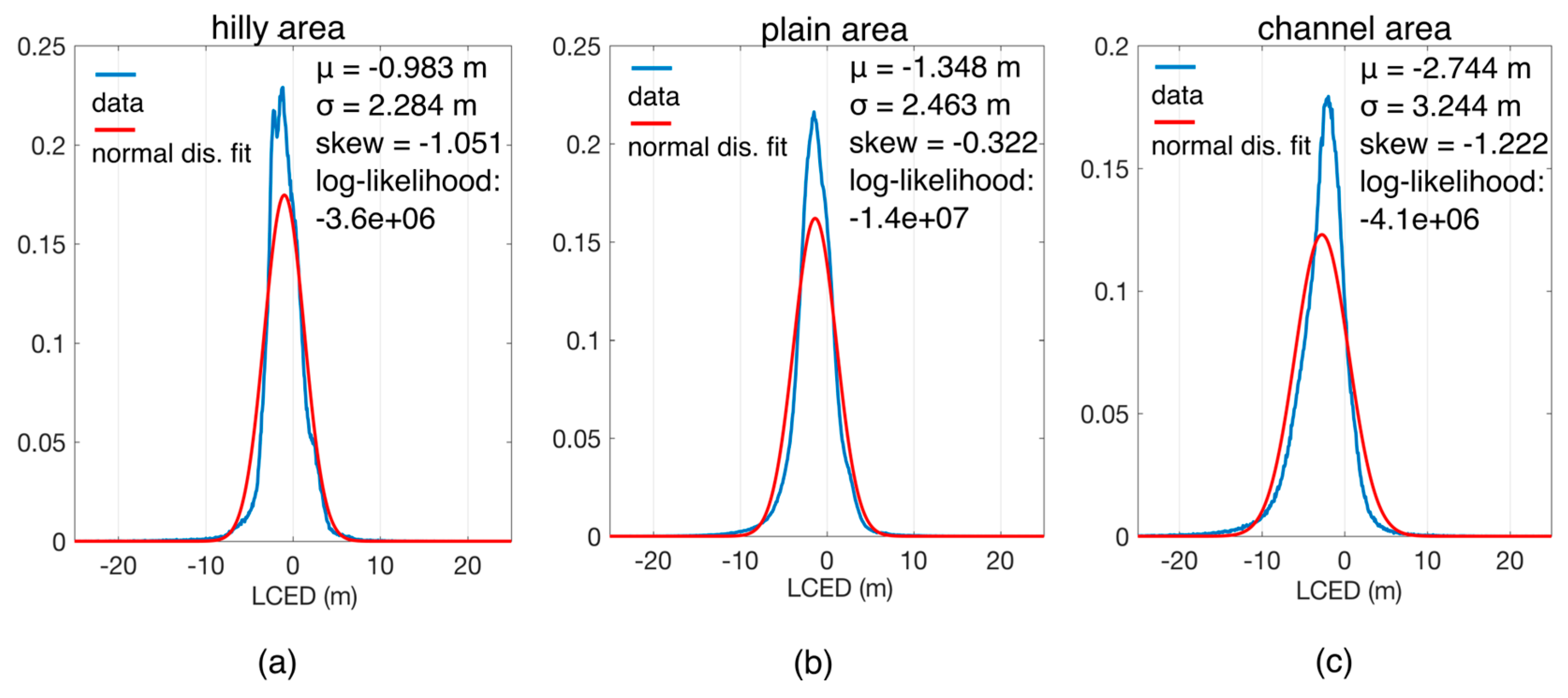
| Statistical Measures | Hilly Area | Plain Area | Channel Area |
|---|---|---|---|
| Numbers of Pixels | 1,610,483 | 6,113,905 | 1,566,449 |
| Area (, km2) | 3336.9 | 12,668.0 | 3175.2 |
| Range from variogram (, km) | 2.2 | ||
| Independent sample numbers () | 1517 | 5758 | 1443 |
| Mean (m) | −0.983 | −1.348 | −2.744 |
| Standard deviation (68.3%) (, m) | 2.284 | 2.463 | 3.244 |
| Standard error of mean (68.3%) (, m) | 0.059 | 0.032 | 0.085 |
© 2017 by the authors. Licensee MDPI, Basel, Switzerland. This article is an open access article distributed under the terms and conditions of the Creative Commons Attribution (CC BY) license (http://creativecommons.org/licenses/by/4.0/).
Share and Cite
Xiong, S.; Muller, J.-P.; Li, G. The Application of ALOS/PALSAR InSAR to Measure Subsurface Penetration Depths in Deserts. Remote Sens. 2017, 9, 638. https://doi.org/10.3390/rs9060638
Xiong S, Muller J-P, Li G. The Application of ALOS/PALSAR InSAR to Measure Subsurface Penetration Depths in Deserts. Remote Sensing. 2017; 9(6):638. https://doi.org/10.3390/rs9060638
Chicago/Turabian StyleXiong, Siting, Jan-Peter Muller, and Gang Li. 2017. "The Application of ALOS/PALSAR InSAR to Measure Subsurface Penetration Depths in Deserts" Remote Sensing 9, no. 6: 638. https://doi.org/10.3390/rs9060638
APA StyleXiong, S., Muller, J.-P., & Li, G. (2017). The Application of ALOS/PALSAR InSAR to Measure Subsurface Penetration Depths in Deserts. Remote Sensing, 9(6), 638. https://doi.org/10.3390/rs9060638