Road Segmentation of Remotely-Sensed Images Using Deep Convolutional Neural Networks with Landscape Metrics and Conditional Random Fields

Abstract

Object segmentation of remotely-sensed aerial (or very-high resolution, VHS) images and satellite (or high-resolution, HR) images, has been applied to many application domains, especially in road extraction in which the segmented objects are served as a mandatory layer in geospatial databases. Several attempts at applying the deep convolutional neural network (DCNN) to extract roads from remote sensing images have been made; however, the accuracy is still limited. In this paper, we present an enhanced DCNN framework specifically tailored for road extraction of remote sensing images by applying landscape metrics (LMs) and conditional random fields (CRFs). To improve the DCNN, a modern activation function called the exponential linear unit (ELU), is employed in our network, resulting in a higher number of, and yet more accurate, extracted roads. To further reduce falsely classified road objects, a solution based on an adoption of LMs is proposed. Finally, to sharpen the extracted roads, a CRF method is added to our framework. The experiments were conducted on Massachusetts road aerial imagery as well as the Thailand Earth Observation System (THEOS) satellite imagery data sets. The results showed that our proposed framework outperformed Segnet, a state-of-the-art object segmentation technique, on any kinds of remote sensing imagery, in most of the cases in terms of $precision$, $recall$, and $F1$.

1. Introduction

Extraction of terrestrial objects such as buildings and roads, from remotely-sensed images has been employed in many applications in various areas, e.g., urban planning, map updates, route optimization, and navigation. For road extraction, most primary research is based on unsupervised learning, such as graph cut and global optimization techniques [1]. These unsupervised methods, however; have one common limitation, color-sensitivity, since they rely on only the color features. That is, the segmentation algorithms will not perform well if the road colors presented in the suburban remotely-sensed images contain more than one color (e.g., yellowish brown roads in the countryside regions and cement-grayed roads in the suburban regions). This, in fact, has become a motivation of this work, that is, to overcome the color sensitivity issues.

Deep learning, a large convolutional neural network with performance that can be scaled depending on the size of training data and model complexity as well as processing power, has shown significant improvements in object segmentation from images as seen in many recent works [2,3,4,5,6,7,8,9,10,11,12,13]. Unlike unsupervised learning, more than one feature—other than color—can be extracted: line, shape, and texture, among others. The traditional deep learning methods such as the deep convolutional neural network (DCNN) [3,14], deep deconvolutional neural network (DeCNN) [5], recurrent neural network, namely reSeg [15], and fully convolutional networks [4]; however all suffer from accuracy performance issues.

A deep convolutional encoder-decoder (DCED) architecture, one of the most efficient newly developed neural networks, has been proposed for object segmentation. The DCED network is designed to be a core segmentation engine for pixel-wise semantic segmentation, and has shown good performance in the experiments tested using PASCAL VOC 2012 data—a well-known benchmark data set for image segmentation research [6,8,16]. In this architecture, the rectified linear unit (ReLU) is employed as an activation function.

In the road extraction task, there are many issues that can cause limited detection performance. First, based on [6,8], although the most recent DCED approach for object segmentation (or SegNet) showed promising detection performance on overall classes, the result for road objects is still limited as it fails to detect many road objects. This could be caused by the rectified linear unit (ReLU) which is sensitive to the gradient vanishing problem. Second, even when we apply Gaussian smoothing at the last step to connect detected roads together, this still yields excessive detected road objects (false road objects).

In this paper, we present an improved deep convolutional encoder-decoder network (DCED) for segmenting road objects from aerial and satellite images. Several aspects of the proposed method are enhanced, including incorporation of exponential linear units (ELUs), as opposed to ReLUs that typically outperform ELU in most object classification cases; adoption of landscape metrics (LMs) to further improve the overall quality of results by removing falsely detected road objects; and lastly, combination with the traditional fully-connected conditional random field (CRF) algorithms used in semantic segmentation problems. Although the ELU-SegNet-LM network may suffer a performance issue due to the loss of spatial accuracy, it can be alleviated by the conditional random fields algorithm, which takes into account the low-level information captured by the local interactions of pixels and edges [17,18,19]. The experiments were conducted using well-known aerial imagery, a Massachusetts roads data set (Mass. Roads), which is publicly available, and satellite imagery (from the Thailand Earth Observation System (THEOS) satellite) which is provided by GISTDA. The results showed that our method outperforms all of the baselines including SegNet in terms of $precision$, $recall$, and $F1$ scores. The paper is organized as follows. Related work is discussed in Section 2. Section 3 describes our proposed methodology. Experimental data sets and evaluations are described in Section 4. Experimental results and discussions are presented in Section 5. Finally, we conclude our work and discuss future work in Section 6.

2. Related Work

Deep learning is one of the fast-growing fields in machine learning which has been successfully applied to remotely-sensed data analysis, notably land cover mapping on urban areas [20]. It has increasingly become a promising tool for accelerating image recognition process with high accuracy results [4], [6], [21]; new architectures are proposed constantly on a weekly basis. This related work is divided into three subsections: we first discuss deep learning concepts for semantic segmentation, followed by a set of road object segmentation techniques using deep learning, and finally activation functions and post processing technique of deep learning are discussed.

Note that this paper only focuses on approaches built around deep learning techniques. Therefore, prior attempts at semantic segmentation [22,23] are not included and compared here since they are not based on a deep learning approach.

2.1. Deep Learning for Semantic Segmentation

Semantic segmentation algorithms are often formulated to solve structured pixel-wise labeling problems based on the deep convolutional neural network (DCNN), and are state-of-the-art supervised learning algorithms for modeling and extracting latent feature hierarchies. Noh et al. [5] proposed a novel semantic segmentation technique utilizing a deconvolutional neural network (DeCNN) and the top layer from DCNN adopted from VGG16 [24]. The DeCNN structure is composed of upsampling layers and deconvolution layers, describing pixel-wise class labels and predicting segmentation masks, respectively. Their proposed deep learning methods yield high performance in the PASCAL VOC 2012 data set [16], with a 72.5% accuracy in the best case scenario (this was the highest accuracy—at the time of writing this paper—compared to other methods that were trained without requiring additional or external data). Long et al. [4] proposed an adapted contemporary classification network incorporating Alex, VGG and Google networks into a full DCNN. In this method, some of the pooling layers were skipped: layer 3 (FCN-8s), layer 4 (FCN-16s), and layer 5 (FCN-32s). The skip architecture reduces the potential over-fitting problem and has shown improvements in performance ranging from 20 to 62.2% in the experiments tested using PASCAL VOC 2012 data. Ronneberger et al. [12] proposed U-Net, a DCNN for biomedical image segmentation. The architecture consists of a contracting path and a symmetric expanding path that capture context and consequently, enable precise localization. The proposed network claimed to be capable of learning despite the limited number of training images, and performed better than the prior best method (a sliding-window DCNN) on the ISBI challenge for segmentation of neuronal structures in electron microscopic stacks. In this work, VGG16 is selected as our baseline architecture since it is the most popular architecture used in various networks for object recognition. Furthermore, we will investigate the effect of the skipped layer technique, especially FCN-8s, since it is the top-ranking architecture as shown in Long et al. [4].

There is a new research area called "instance-aware semantic segmentation" which is slightly different from "semantic segmentation." Instead of labeling all pixels, it focuses on the target objects and labels only pixels of those objects. FCIS [25] is a technique developed based on fully convolutional networks (FCN). Mask R-CNN [26] is also created on top of FCN but incorporates with a proposed joint formulation. Even though their results are promising, they are not directly related to our scope on "semantic segmentation." In the future, we can extend these works and compare them to our proposed technique.

2.2. Deep Learning for Road Segmentation

There are many approaches to road network extraction in very-high-resolution (VHR) aerial and satellite imagery literature. Wand et al. [14] proposed a DCNN and finite state machine (FSM)-based framework to extract road networks from aerial and satellite images. DCNN recognizes patterns from a sophisticated and arbitrary environment while FSM translates the recognized patterns to states such that their tracking behaviors can be captured. The results showed that their approach is more accurate compared to the traditional methods. The extension of the method for automatic road point initialization was left for future work. DCNN for multiple object extraction from aerial imagery was proposed in [3] by Saito et al. Both features (extractors and classifiers) of DCNN were automated in that a new technique to train a single DCNN for extracting multiple kinds of objects simultaneously was developed. Two objects were extracted: buildings and roads, thus a label image consists of three channels: buildings, roads, and background. Finally, the results showed that the proposed technique not only improved the prediction performance but also outperformed the cutting-edge method tested on a publicly available aerial imagery data set. Muruganandham et al. [2] designed an automated framework to extract semantic maps of roads and highways, so the urban growth of cities from remote sensing images could be tracked. They used the VGG16 model—a simplistic architecture with homogeneous 3 × 3 convolution kernels and 2 × 2 max pooling throughout the pipeline—as a baseline for a fixed feature extractor. The experimental results showed that their proposed technique for the prediction performance was improved with $F1$ scores of 0.76 on the Mass. Roads data set.

2.3. Recent Techniques in Deep Learning

Activation function is an important factor for the accuracy of DCNN. While the most popular activation function for neural networks is the rectified linear unit (ReLU), Clevert et al. [21] have just proposed the exponential linear unit (ELU), which can speed up the learning process in DCNN and therefore lead to higher classification accuracies as well as overcoming the previously unsolvable problem, i.e., the vanishing gradient problem. Compared to other methods with different activation functions, ELU has greatly improved many of the learning characteristics. In the experiments, ELUs enable fast learning as well as more effective generalization performance than the ReLUs and the leaky rectified linear units (LReLUs) in networks with five layers or more. In ImageNet, ELU networks substantially increased the learning time compared to ReLU networks with the identical architecture; less than 10% classification error was presented for a single crop, model network.

Recently, there have been some efforts to enhance the performance of DCNN by combining it with other classifier as a post-processing step. Conditional random fields (CRFs) has been reported successful in increasing the accuracy of DCNN, especially in the image segmentation domain. CRFs have been employed to smooth maps [7,17,18,19]. Typically these models contain energy terms that couple neighboring nodes, favoring same-label assignments to spatially proximal pixels. Qualitatively, the primary function of these short-range CRFs has been used to clean up the spurious predictions of weak classifiers built on top of local hand-engineered features.

3. Proposed Methodology

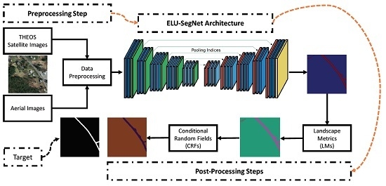
In this section, we propose an enhanced, improved DCED network (or SegNet) to efficiently segment road objects from aerial and satellite images. Three aspects of the proposed method are enhanced: (1) modification of DCED architecture; (2) incorporation of landscape metrics (LMs); and (3) adoption of conditional random fields (CRFs). An overview of our proposed method is shown in Figure 1.

Figure 1. A process in our proposed framework.

3.1. Data Preprocessing

Data preparation is required when working with neural network and deep learning models. In addition, data augmentation is often required in more complex object recognition tasks. Thus, we increased the size of our data sets to improve the method efficiency by rotating them incrementally with eight different angles. All images on Massachusetts road data sets are standardized and cropped into 1500 × 1500 pixels with a resolution of 1 m${}^2$/pixel. The data sets consist of 1108 training images, 49 test images, and 14 validation images. The original training images were further extended to 8864 training images.

On the THEOS data sets, we also increased the size of data sets in a similar fashion. Each image has 1500 × 1500 pixels with a resolution of 2 m${}^2$/pixel.

3.2. Object Segmentation (ELU-SegNet)

SegNet, one of the deep convolutional encoder-decoder architectures, consists of two main networks encoder and decoder, and some outer layers. The two outer layers of the decoder network are responsible for feature extraction task, the results of which are transmitted to the next layer adjacent to the last layer of the decoder network. This layer is responsible for pixel-wise classification (determining which pixel belongs to which class). There is no fully connected layer in between feature extraction layers. In the upsampling layer of decoder, pool indices from encoder are distributed to the decoder where the kernel will be trained in each epoch (training round) at the convolution layer. In the last layer (classification), softmax is used as a classifier for pixel-wise classification. The encoder network consists of convolution layer and pooling layer. A technique, called batch normalization (proposed by Ioffe and Szegedy [27]), is used to speed up the learning process of the DCNN by reducing internal covariate shift. In the encoder network, the number of layers is reduced to 13 (VGG16) by removing the last three layers (fully connected layers) [6,8,28,29] for the following two reasons: to maintain the high-resolution feature maps in the encoder network, and to minimize the countless number of parameters from 134 million features to 14.7 million features compared to the traditional deep learning networks such as DCNN [4] and DeCNN [5], where the fully connected layer remains intact. In the activation function of feature extraction, ReLU, max-pooling, and 7 × 7 kernels are used in both encoder and decoder networks. For training images, three-channel images (RGB) are used. The exponential linear unit (ELU) was introduced in [21], which can speed up learning in deep neural networks, offer higher classification accuracies, and give better generalization performance than ReLUs and LReLUs on networks. In SegNet architecture, to perform optimization for training networks,the stochastic gradient descent (SGD) [30] with a fixed learning rate of 0.1 and momentum of 0.9 is used. In each training round (epoch), a mini-batch (a set of 12 images) is chosen such that each image is used once. The model with the best performance on the validation data set in each epoch will be selected. Our architecture (see Figure 2) is enhanced from SegNet, consisting of two main networks responsible for feature extraction. In each network, there are 13 layers, with the last layer being the classification based on softmax supporting pixel-wise classification.

Figure 2. A proposed network architecture for object segmentation (exponential linear unit (ELU)-SegNet).

In our work, an activation function called ELU is used as opposed to ReLU based on its performances. For the network training optimization, stochastic gradient descent (SGD) is used and configured with a fixed learning rate of 0.001 and momentum of 0.9 to delay the convergence time and so, can avoid local optimization trap.

3.3. Gaussian Smoothing

Gaussian smoothing [31] is a 2-D convolution operator that is used to ‘blur’ images and remove unnecessary details and noises by utilizing the Gaussian function. The Gaussian function is used to determine the transformation needed for each pixel, resulting in a more complete extended road objects. We applied the Gaussian function first in the post-processing step in order to expand and prepare objects that are close to each other to be combined into components in the next step (as we shall see in Section 3.4).

The 1-D and 2-D Gaussian functions are described in Equations (1) and (2), respectively.

$$G\left(x\right)=\frac{1}{2\pi {\sigma }^2}{e}^{-\frac{x^2}{2{\sigma }^2}}$$

(1)

$$G\left(x\right)=\frac{1}{2\pi {\sigma }^2}{e}^{\frac{-x^2-y^2}{2{\sigma }^2}}$$

(2)

where x represents the distance from the origin in the X-axis, y represents the distance from the origin in the Y-axis, and $\sigma$ represent the standard deviation of the Gaussian distribution.

3.4. Connected Component Labeling (CCL)

In connected components labeling (CCL) [31], all pixels are scanned and adjacent pixels with similar connectivity values are combined. Eight neighbors of each pixel were considered when analyzing connected components.

The expanded and overlapped objects from the Gaussian smoothing were actually grouped together in this step. The labeled objects will be further calculated using geometric attributes (e.g., area and perimeter) based on landscape metrics (LMs) as described in the next section.

3.5. False Road Object Removal (LMs)

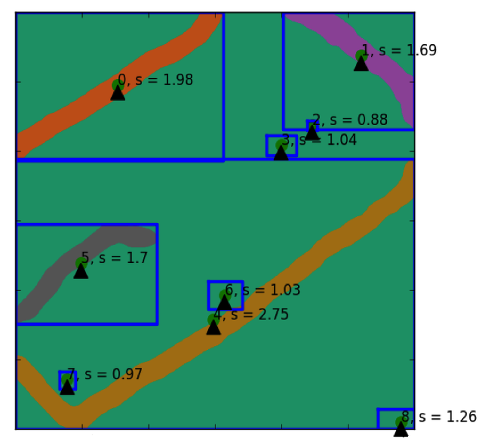
After smoothing and labeling the objects, we compute the shape complexity of the objects through the shape index (as seen in Equation (3)), one of the landscape metrics for measuring arrangement and composition property of spatial objects. The resulting objects along with their shape scores are shown in Figure 3. As seen in Figure 3, the geometrical characteristics of roads were captured and differentiated from other spatial objects in the given image. Other geometry metrics can also be used such as rectangular degree, aspect ratio, etc. More information on other landscape metrics can be found in [32,33].

$$shapeindex=\frac{e\left(i\right)}{4x\sqrt{A\left(i\right)}}$$

(3)

where $e\left(i\right)$ and $A\left(i\right)$ denote the perimeter and area for object i, respectively.

Figure 3. Illustration of shape index scores on each extracted road object. Any objects with shape index score lower than 1.25 are considered as noises and subsequently removed.

3.6. Road Object Sharpening (CRFs)

Conditional random fields (CRFs) have traditionally been implemented to sharpen noisy segmentation maps [18]. These models are generally composed of energy terms comprising nodes in the neighborhood, causing false assignments of pixels that are in close proximity. To resolve these spatial limitations of short-range CRFs, the fully connected CRFs are integrated into our system [19]. Equation (4) expresses the energy function of the dense CRFs.

In the last step, we extended the ELU-SegNet-LMs model to ELU-SegNet-LMs-CRFs to enhance the network performance by adding explicit dependencies among the neural network outputs. Particularly, we added smoothness terms between neighboring pixels to our model, which can eliminate the need to learn smoothness from remotely-sensed images. Using the resulting models as part of the post-processing significantly increases the overall performance of the network over unstructured deep neural networks.

$$E\left(x\right)=\sum _i{\theta }_i\left(x_i\right)+\sum _{ij}{\theta }_{ij}(x_i,x_j)$$

(4)

where x denotes the label assignment for pixels. A unary potential used is ${\theta }_i\left(x_i\right))=-logP\left(x_i\right)$, while $P\left(x_i\right)$ denotes the label assignment probability at pixel i as computed by a DCNN.

The inference can be efficiently established in the pair-wise potentials when using the fully connected graph. We treated the unary potential as local classifiers which are defined by the output of the ELU-SegNet-LMs model, which is a probability map for each class in each of the pixels. The pairwise potentials depict the interaction of pixels in the neighborhood and are influenced by the color similarity. In the DeepLab CRF model [19], the dense CRFs (instead of neighboring information) are used as a means to identify relationships between pixels. Furthermore, they define the following pairwise potentials as shown in Equation (5).

$${\theta }_{ij}(x_i,x_j)=\mu (x_i,x_j)[w_{1}exp(-{\frac{\parallel p_i-p_j\parallel }{2{\sigma }_{\alpha }^2}}^2-{\frac{\parallel I_i-I_j\parallel }{2{\sigma }_{\beta }^2}}^2)+w_{2}exp(-\frac{{\parallel p_i-p_j\parallel }^2}{2{\sigma }_{\gamma }^2})]$$

(5)

where $\mu (x_i,x_j)=1if{x}_i\ne x_j$ and zero otherwise, which, as in the Potts model, means that only nodes with distinct labels are penalized. The remaining expression uses two Gaussian kernels in different feature spaces; the first, ’bilateral’ kernel depends on both pixel positions (denoted as p) and red-green-blue (RGB) color (denoted as I), and the second kernel only depends on pixel positions. The hyperparameters ${\sigma }_{\alpha },{\sigma }_{\beta }and{\sigma }_{\gamma }$ control the scale of Gaussian kernels. The first kernel forces pixels to similar color and position to have similar labels, while the second kernel only considers spatial proximity when enforcing smoothness.

In summary, the first term of pairwise potentials depends on both pixel positions and color intensities whereas the second term depends solely on the pixel positions [18,19]. Although the dense CRFs can have billions of edges (which is technically infeasible to solve), it was recently found that the inference/maximum posterior can be approximated by the mean-field algorithm.

4. Experimental Data Sets and Evaluation

In our experiments, two types of data sets are used: aerial images and satellite images. Table 1 shows one aerial data set (Massachusetts) and five satellite data sets (Nakhonpathom, Chonburi, Songkhla, Surin, and Ubonratchathani). All experiments are evaluated based on $precision$, $recall$, and $F1$.

Table 1. Numbers of training, validation, and testing sets.

	Training Set	Validation Set	Testing Set
Massachusetts	1108	14	49
Nakhonpathom	200	14	49
Chonburi	100	14	49
Songkhla	100	14	49
Surin	70	14	49
Ubonratchathani	70	14	49

4.1. Massachusetts Road Data Set (Aerial Imagery)

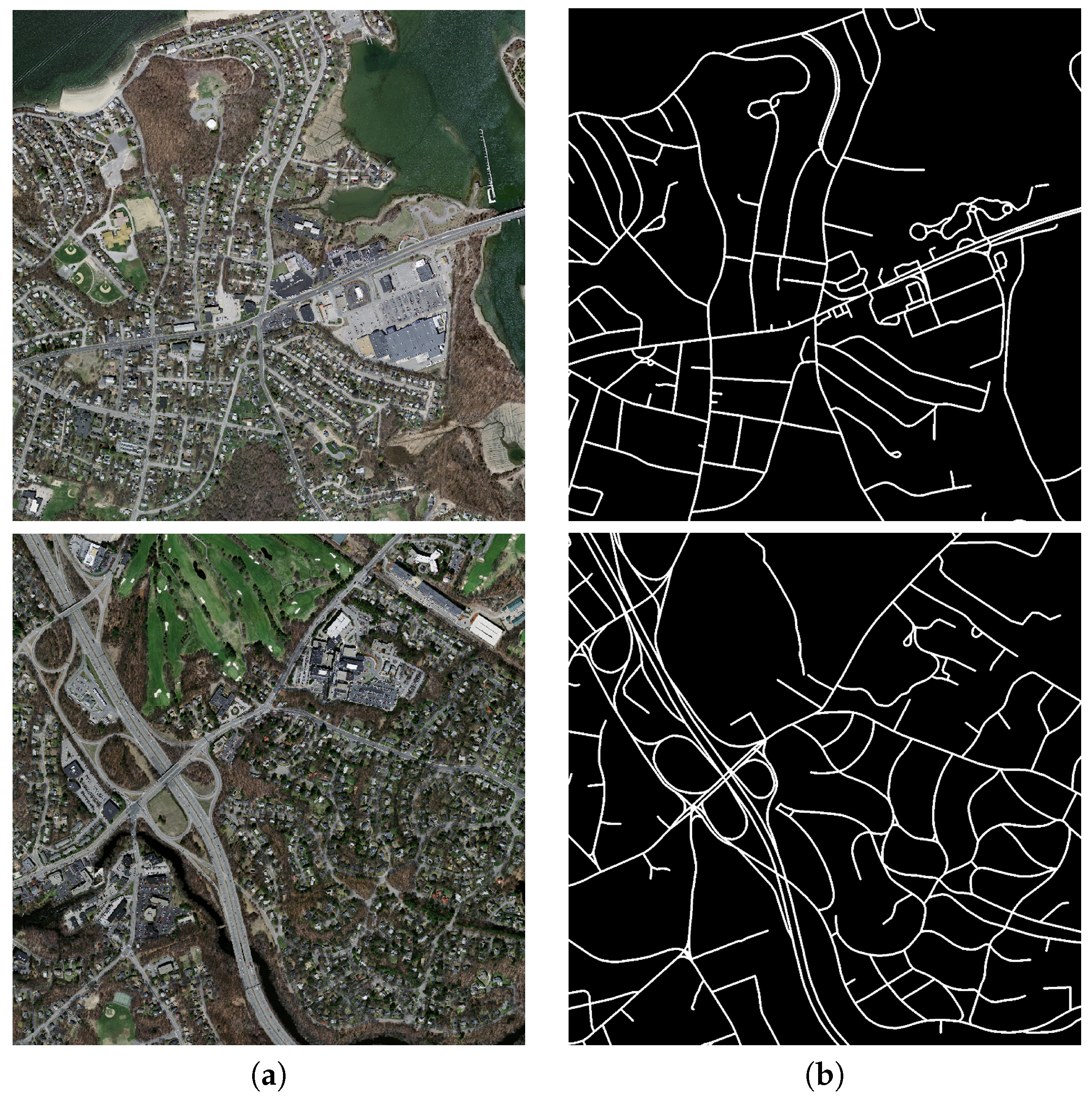
This data set (made publicly available by [7]) consists of 1171 aerial images of the state of Massachusetts. Each image is 1500 × 1500 pixels in size, covering an area of 2.25 square kilometers. We randomly split the data into a training set of 1108 images, a validation set of 14 images and a testing set of 49 images. The samples of this data set are shown in Figure 4. The data set covers a wide variety of urban, suburban, and rural regions with a total area of over 2600 square kilometers. With our test set alone, it covers more than 110 square kilometers which is by far the largest and most challenging aerial image labeling data set.

Figure 4. Two sample aerial images from the Massachusetts road corpus, where a row refers to each image (a) Aerial image and (b) Binary map, which is a ground truth image denoting the location of roads.

4.2. THEOS Data Sets (Satellite Imagery)

In this type of data, the satellite images were separated into five data sets—one for each province. The datasets were obtained from the Thailand Earth Observation System (THEOS), also known as Thaichote, an Earth observation satellite of Thailand developed by EADS Astrium SAS, France. This data set consists of 855 satellite images covering five provinces: 263 images of Nakhonpathom, 163 images of Chonburi, 163 images of Songkhla, 133 images of Surin, and 133 images of Ubonratchathani. Some samples of these images are shown in Figure 5.

Figure 5. Sample satellite images from five provinces of our data sets; each row refers to a single sample image from one province (Nakhonpathom, Chonburi, Songkhla, Surin, and Ubonratchathani) in a satellite image format (a) and in a binary map (b), which is served as a ground truth image denoting the location of roads.

4.3. Evaluation

The road extraction task can be considered as binary classification, where road pixels are positives and the remaining non-road pixels are negatives. Let TP denote the number of true positives (the number of correctly classified road pixels), TN denote the number of true negatives (the number of correctly classified non-road pixels), FP denote the number of false positives (the number of mistakenly classified road pixels), and FN denote the number of false negatives (the number of mistakenly classified non-road pixels).

The performance measures used are $precision$, $recall$, and $F1$ as shown in Equations (6)–(8). Precision is the percentage of correctly classified road pixels among all predicted pixels by the classifier. Recall is the percentage of correctly classified road pixels among all actual road pixels. $F1$ is a combination of precision and recall.

$$Precision=\frac{TP}{TP+FP}$$

(6)

$$Recall=\frac{TP}{TP+FN}$$

(7)

$$F1=\frac{2\times Precision\times Recall}{Precison+Recall}$$

(8)

5. Experimental Results and Discussions

This section illustrates details of our experiments. The proposed deep learning network is based on SegNet with three improvements: (1) it employs the ELU activation function; (2) it uses LMs to filter incorrect detected roads; and (3) it applies CRFs to sharpen broad roads. Thus, there are three variations of the proposed methods as shown in Table 2.

Table 2. Variations of our proposed deep learning methods. LM: landscape metric; CRF: conditional random field.

Abbreviation	Description
ELU-SegNet	SegNet + ELU activation
ELU-SegNet-LMs	SegNet + ELU activation + Landscape Metrics
ELU-SegNet-LMs-CRFs	SegNet + ELU activation + Landscape Metrics + CRFs

For the experimental setup, there are three experiments on two remotely-sensed data sets: the Massachusetts road data set and THEOS data sets (details in Section 4). The experiments aim to illustrate that each proposed strategy can really improve the performance. First, ELU-SegNet is compared to SegNet for the ELU strategy. Second, ELU-Segnet-LMs is compared to ELU-SegNet for the LM strategy. Third, the full proposed technique (ELU-Segnet-LMs-CRFs) is compared to existing methods for the CRF technique.

The implementation is based on a deep learning framework, called “Lasagne”, which is extended from Theano. All experiments were conducted on a server with Intel Core i5-4590S Processor (6M Cache, up to 3.70 GHz), 32 GB of memory, Nvidia GeForce GTX 960 (4 GB), and Nvidia GeForce GTX 1080 (8 GB). Instead of using the whole image (1500 × 1500 pixels) to train the network, we randomly cropped all images to be 224 × 224 as inputs of each epoch.

5.1. Results on Aerial Imagery (Massachusetts Data Set)

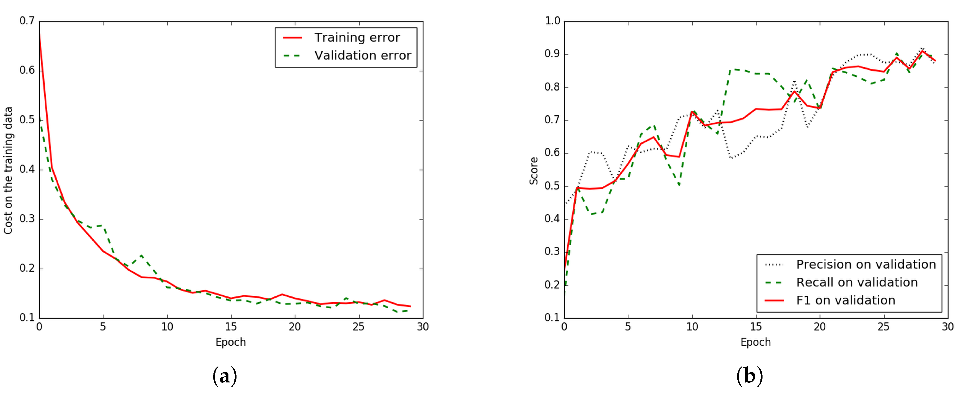
In this sub-section, the experiment was conducted on the Massachusetts aerial corpus. To achieve the highest accuracy, the network must be configured and trained many epochs until all parameters in the network are converged. Figure 6a illustrates that the proposed network has been properly set and trained until it really is converged. Furthermore, Figure 6b shows that the higher number of epochs tends to show a better $F1$-score. Thus, the number of chosen epochs based on the validation data is 29 (the best model for this data set).

Figure 6. Iteration plot on Massachusetts aerial corpus of the proposed technique, ELU-SegNet-LMs-CRFs; x refers to epochs and y refers to different measures. (a) Plot of model loss (cross entropy) on training and validation data sets, and (b) Performance plot on the validation data set.

The result is shown in Table 3 by comparing between baselines and variations of the proposed techniques. It shows that our network with all strategies (ELU-SegNet-LMs-CRFs) outperforms other methods. More details will be discussed to show that each of the proposed techniques can really improve an accuracy. Only in this experiment, there are four baselines, including Basic-model, FCN-no-skip, FCN-8s, and SegNet. Note that SegNet has been implemented and tested on the experimental data set, while the results of other three baselines are carried from the original paper [2].

Table 3. Results on the testing data of Massachusetts aerial corpus between four baselines and three variations of our proposed techniques in terms of $precision$, $recall$, and $F1$. FCN: fully convolutional network.

	Model	Precsion	Recall	F1
Baselines	Basic-model [2]	0.657	0.657	0.657
	FCN-no-skip [2]	0.742	0.742	0.742
	FCN-8s [2]	0.762	0.762	0.762
	SegNet	0.773	0.765	0.768
Proposed Method	ELU-SegNet	0.852	0.733	0.788
	ELU-SegNet-LMs	0.854	0.861	0.857
	ELU-SegNet-LMs-CRFs	0.858	0.894	0.876

5.1.1. Results of Enhanced SegNet (ELU-SegNet)

Our first strategy aims to increase an accuracy of the network by using ELU as an activation function (ELU-SegNet) rather than the traditional one, ReLU (SegNet). Details are shown in Section 3.2. From Table 3, $F1$ of ELU-SegNet (0.788) outperforms that of SegNet (0.768); this yields higher $F1$ at 2.6%. The main reason is due to higher $precision$, but slightly lower $recall$. This can imply that ELU is more robust than ReLU to detect road pixels.

5.1.2. Results of Enhanced SegNet with Landscape Metrics (ELU-SegNet-LMs)

Our second mechanism focuses on applying LMs (details in Section 3.5) on top of ELU-SegNet to filter false road objects. From Table 3, the $F1$ of ELU-SegNet-LMs (0.857) is superior to that of ELU-SegNet (0.788) and SegNet (0.768); this yields higher $F1$ at 6.9% and 8.9%, consecutively. Although LM is specifically designed to increase $precision$, the result shows that it can increase both $precision$ (0.854) and $recall$ (0.861). It is interesting that $recall$ is also improved since all noises in the training images have been removed by the LMs filtering technique resulting in a better quality of the training data set.

5.1.3. Results of All Modules (ELU-SegNet-LMs-CRFs)

Our last strategy aims to sharpen road objects (details in Section 3.6) by integrating CRFs into our deep learning network. From Table 3, $F1$ of ELU-SegNet-LMs-CRFs (0.876) is the winner; it clearly outperforms not only the baselines, but also all previous generations. Its $F1$ is higher than SegNet (0.768) at 10.8%. Also, the result illustrates that CRFs can enhance both $precision$ (0.858) and $recall$ (0.894).

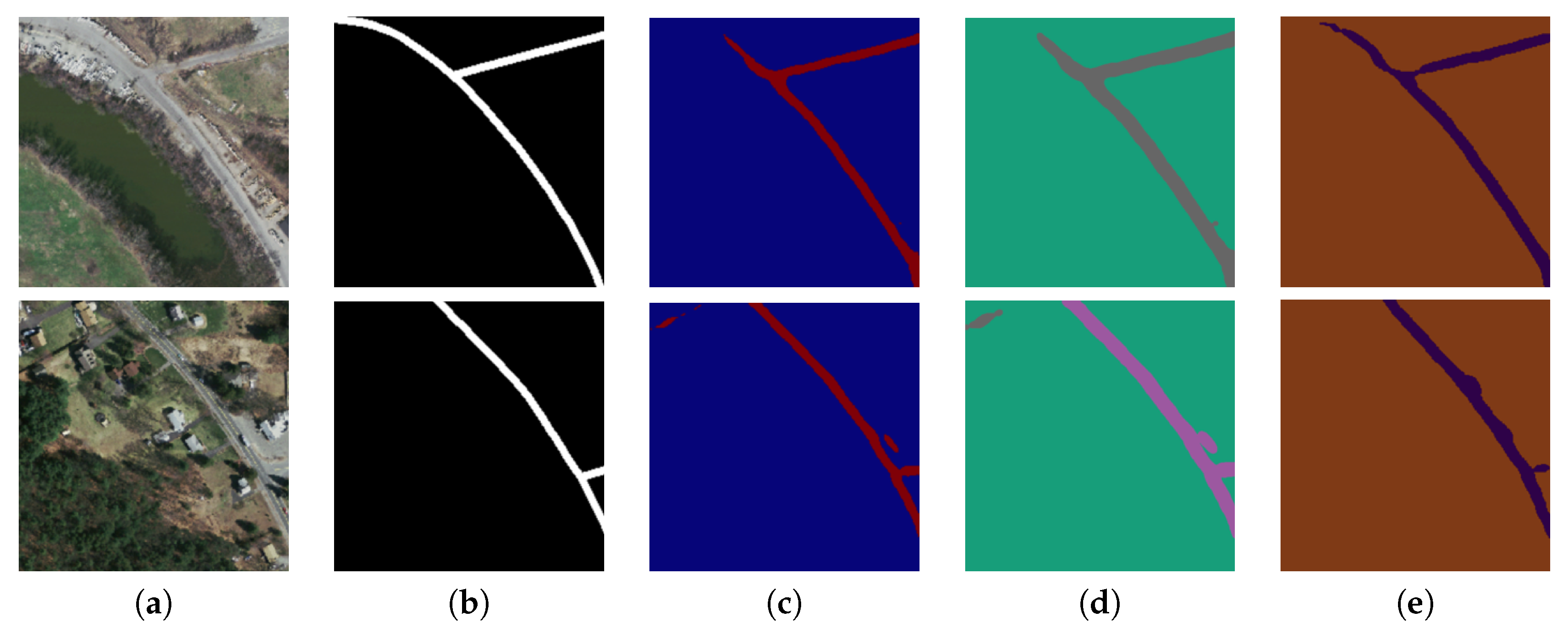
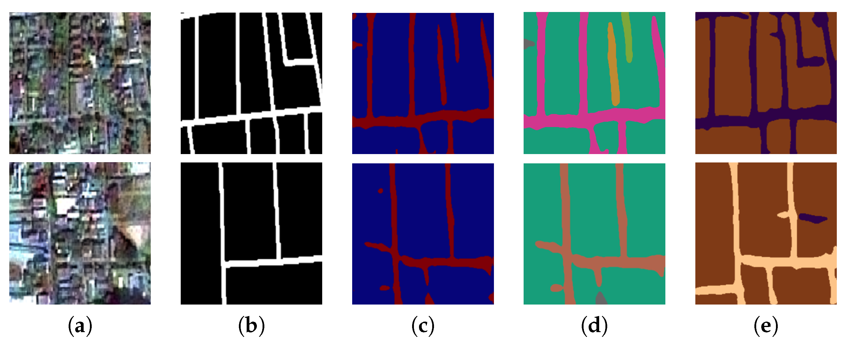
Figure 7 shows two sample results from the proposed method. By applying all strategies, the images in the last column (Figure 7e) look very close to the ground truths (Figure 7b). Furthermore, $F1$-results are improved for each strategy we added to the network as shown in Figure 7c–e.

Figure 7. Two sample input and output aerial images on Massachusetts corpus, where rows refer different images. (a) Original input image; (b) Target road map (ground truth); (c) Output of ELU-SegNet; (d) Output of ELU-SegNet-LMs; and (e) Output of ELU-SegNet-LMs-CRFs.

5.2. Results for Satellite Imagery (THEOS Data Sets)

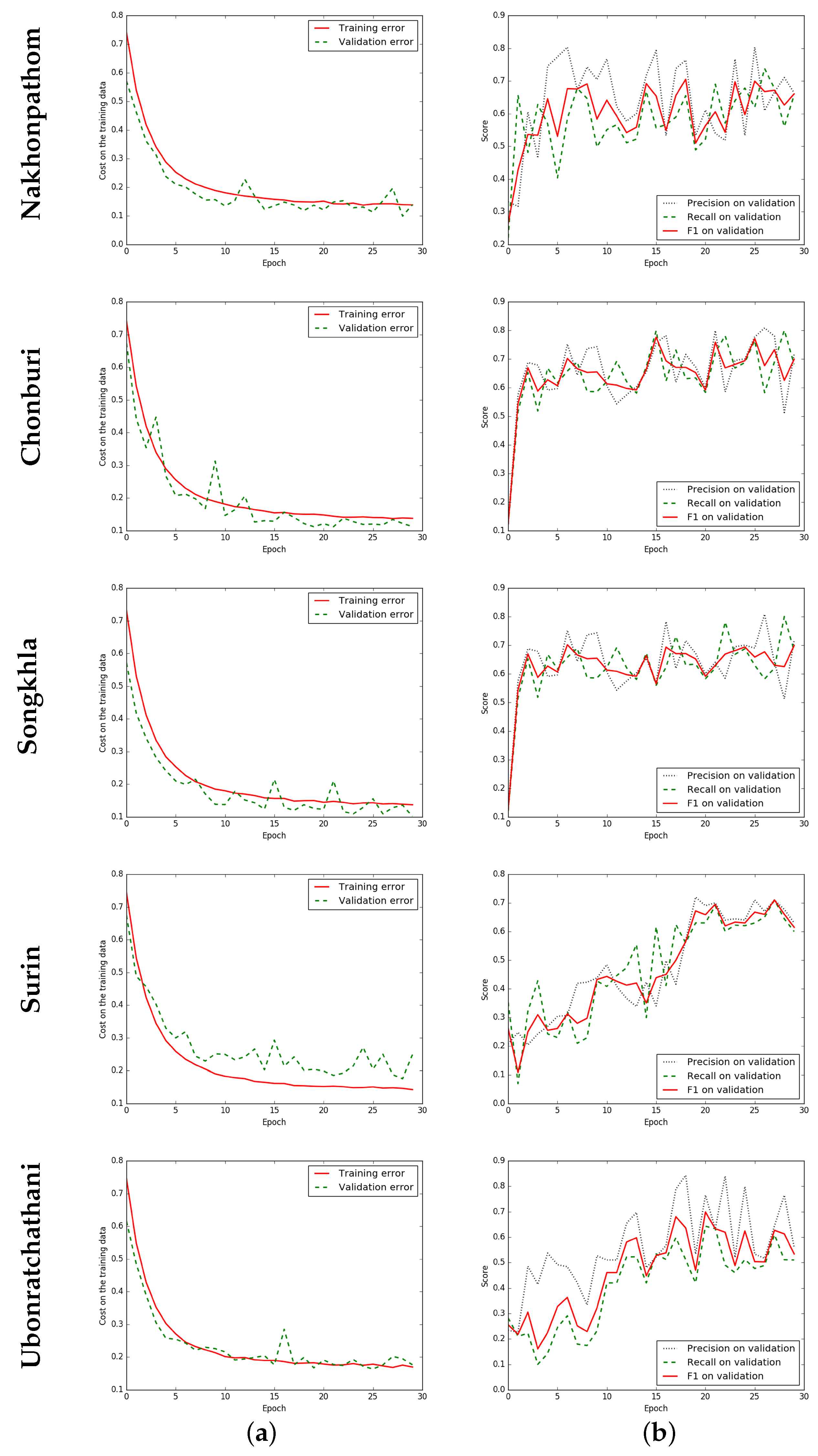
In this sub-section, the experiment was conducted on THEOS satellite images. There are five data sets referring to different provinces: Nakhonpathom, Chonburin, Songkla, Surin, and Ubonratchathani; therefore, there are five learning models. Figure 8 shows that each model is properly set up and trained until it is converged and obtained the best $F1$. The best epochs (models) for each province are 25, 15, 30, 21, and 20, respectively.

Figure 8. Iteration plot on THEOS satellite data sets of the proposed technique, ELU-SegNet-LMs-CRFs. x refers to epochs and y refers to different measures. Each row refers to different data set (province). (a) Plot of model loss (cross entropy) on training and validation data sets; and (b) Performance plot on the validation data set.

The results are shown in Table 4, Table 5 and Table 6 for measures in terms of $F1$, $precision$, and $recall$, respectively. It is interesting that the proposed network with all strategies (ELU-SegNet-LMs-CRFs) is the winner showing the best performance on any measures and provinces. Also, an improvement in the satellite images is higher than that in the aerial images. More details on each proposed strategy will be discussed.

Table 4. $F1$ on the testing data of the Thailand Earth Observation System (THEOS) satellite data sets between baseline (SegNet) and three variations of our proposed techniques; columns refer to five different provinces (data sets).

	Model	Nakhon.	Chonburi	Songkhla	Surin	Ubon.	Avg.
Baseline	SegNet	0.422	0.572	0.424	0.501	0.406	0.465
Proposed Method	ELU-SegNet	0.463	0.690	0.497	0.591	0.534	0.555
	ELU-SegNet-LMs	0.488	0.732	0.526	0.625	0.562	0.587
	ELU-SegNet-LMs-CRFs	0.550	0.775	0.607	0.707	0.608	0.649

Table 5. $precision$ on the testing data of THEOS satellite data sets between baseline (SegNet) and three variations of our proposed techniques; columns refer to five different provinces (data sets).

	Model	Nakhon.	Chonburi	Songkhla	Surin	Ubon.	Avg.
Baseline	SegNet	0.435	0.668	0.456	0.598	0.601	0.552
Proposed Method	ELU-SegNet	0.410	0.702	0.478	0.840	0.852	0.656
	ELU-SegNet-LMs	0.494	0.852	0.557	0.770	0.867	0.708
	ELU-SegNet-LMs-CRFs	0.535	0.909	0.650	0.786	0.871	0.751

Table 6. $recall$ on the testing data of THEOS satellite data sets between baseline (SegNet) and three variations of our proposed techniques; columns refer to five different provinces (data sets).

	Model	Nakhon.	Chonburi	Songkhla	Surin	Ubon.	Avg.
Baseline	SegNet	0.410	0.499	0.395	0.431	0.306	0.408
Proposed Method	ELU-SegNet	0.532	0.678	0.517	0.456	0.389	0.515
	ELU-SegNet-LMs	0.483	0.642	0.498	0.526	0.416	0.513
	ELU-SegNet-LMs-CRFs	0.566	0.676	0.570	0.643	0.467	0.584

5.2.1. Results of Enhanced SegNet (ELU-SegNet)

The ELU activation function can increase the performance of the network. In terms of $F1$, Table 4 shows that ELU-SegNet outperforms the traditional network (SegNet) for all provinces. It performs better than SegNet by 9.08% on average for all provinces, where Ubonratchathani and Chonburi show the highest $F1$-improvement, at over 10%. For $precision$ and $recall$, Table 5 and Table 6 illustrate that almost all data sets can be improved employing the ELU function with improvements of 10.48% and 10.68% on average for all provinces, respectively, .

5.2.2. Results of Enhanced SegNet with Landscape Metrics (ELU-SegNet-LMs)

The LMs filtering strategy aims to remove all inaccurately extracted roads (false positives: FP) resulting in higher $precision$ and $F1$, but this might imply a slight loss in $recall$. Comparing to the previous generation (ELU-SegNet), there are improvements by LMs on average for all provinces of 5.2% and 3.2% in terms of $precision$ (Table 5) and $F1$ (Table 4), respectively, with a slight loss of −0.22% in terms of $recall$ (Table 6). Compared to the baseline, LMs outperforms SegNet on all performance measures.

5.2.3. Results of All Modules (ELU-SegNet-LMs-CRFs)

To further improve the performance, CRFs is integrated into the network from the previous section. This is considered to use all proposed modules: ELU, LMs, and CRFs. From Table 4, Table 5 and Table 6, the results show that ELU-SegNet-LMs-CRFs is the winner compared the previous generations and baseline (SegNet) on any of the measures ($precision$, $recall$, and $F1$). As of $F1$ average of all provinces, it outperforms ELU-SegNet-LMs, ELU-SegNet, and SegNet by 6.28%, 9.44% and 18.44%, respectively.

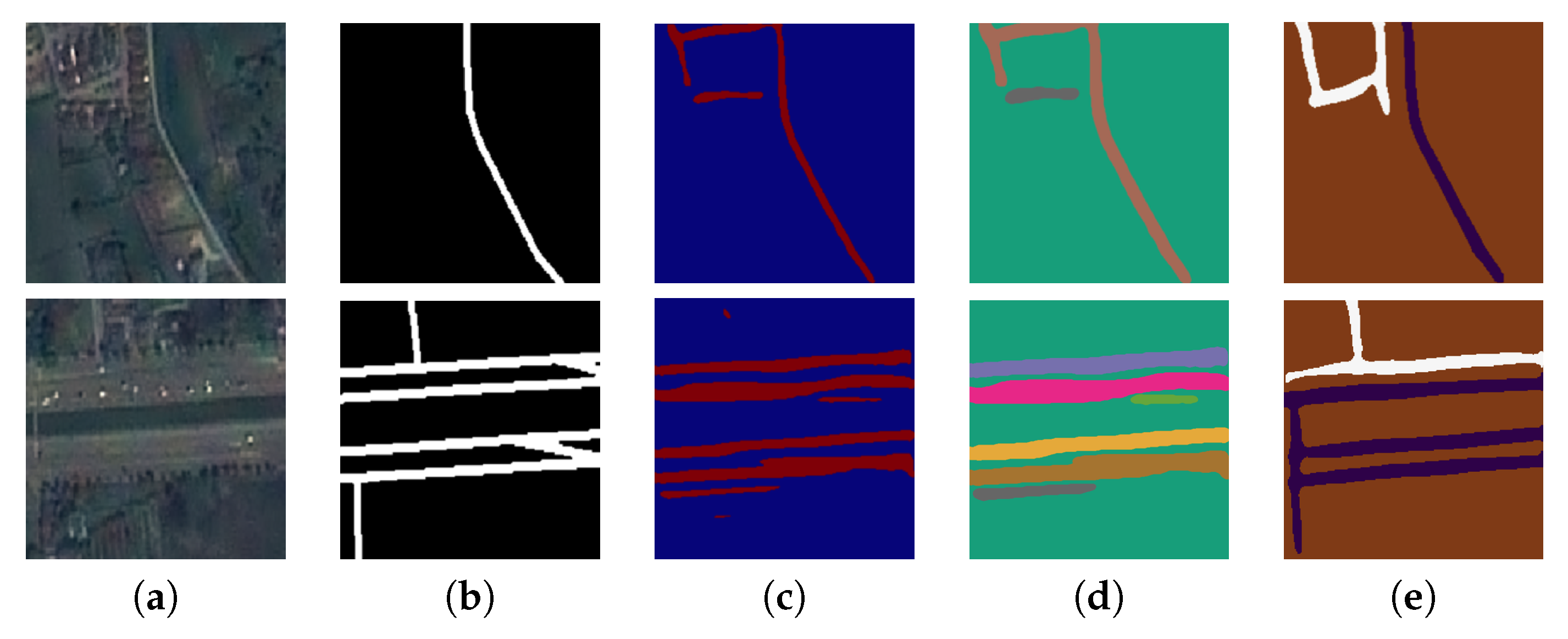
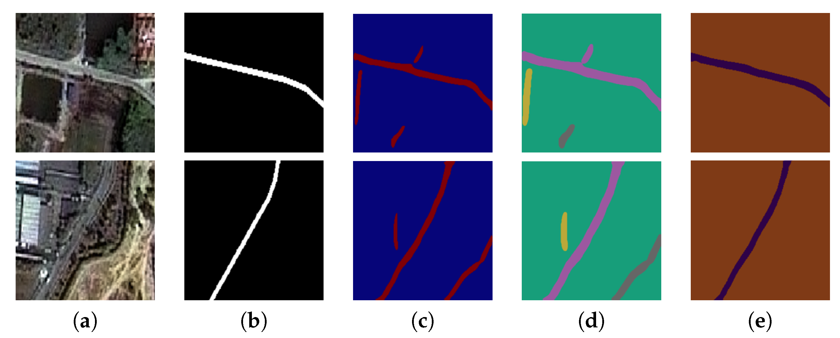
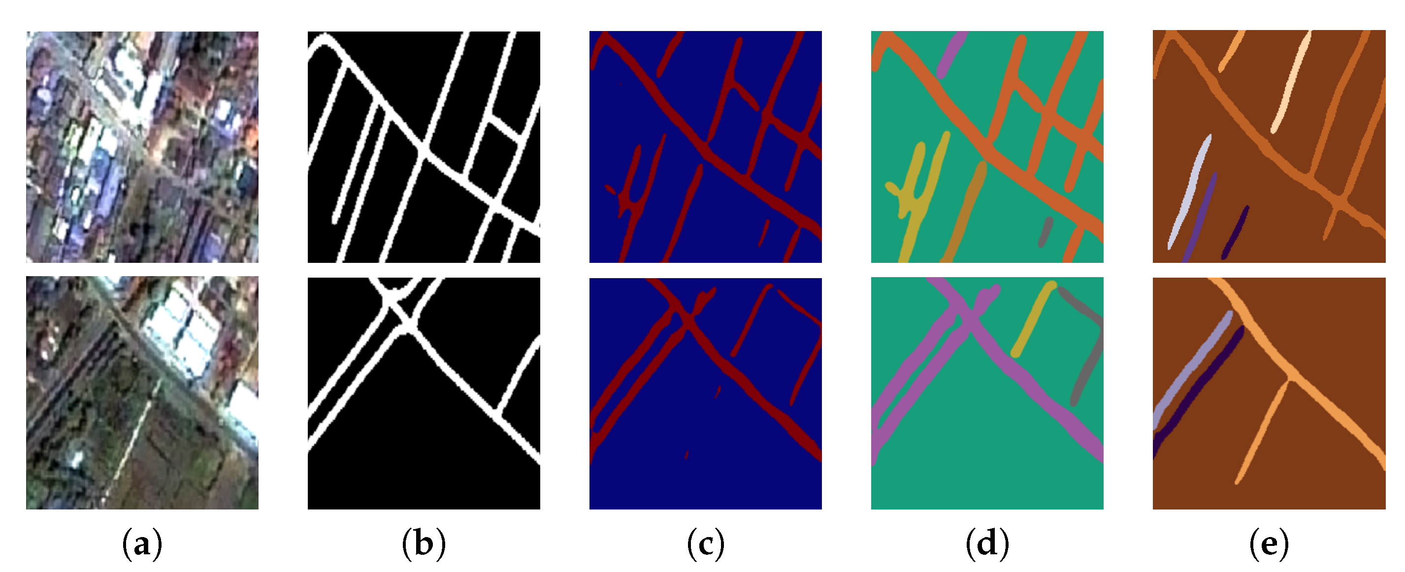
Figure 9, Figure 10, Figure 11, Figure 12 and Figure 13 show sample results from the proposed method on five provinces. The results of the last column look closest to the ground truth in the second column.

Figure 9. Two sample input and output THEOS satellite images on the Nakhonpathom data set, where rows refer different images. (a) Original input image; (b) Target road map (ground truth); (c) Output of ELU-SegNet; (d) Output of ELU-SegNet-LMs; and (e) Output of ELU-SegNet-LMs-CRFs.

Figure 10. Two sample input and output THEOS satellite images on the Chonburi data set, where rows refer different images. (a) Original input image; (b) Target road map (ground truth); (c) Output of ELU-SegNet; (d) Output of ELU-SegNet-LMs; and (e) Output of ELU-SegNet-LMs-CRFs.

Figure 11. Two sample input and output THEOS satellite images on the Songkhla data set, where rows refer different images. (a) Original input image; (b) Target road map (ground truth); (c) Output of ELU-SegNet; (d) Output of ELU-SegNet-LMs; and (e) Output of ELU-SegNet-LMs-CRFs.

Figure 12. Two sample input and output THEOS satellite images on the Surin data set, where rows refer different images. (a) Original input image; (b) Target road map (ground truth); (c) Output of ELU-SegNet; (d) output of ELU-SegNet-LMs; and (e) Output of ELU-SegNet-LMs-CRFs.

Figure 13. Two sample input and output THEOS satellite images on Ubonratchathani data set, where rows refer different images. (a) Original input image; (b) Target road map (ground truth); (c) Output of ELU-SegNet; (d) Output of ELU-SegNet-LMs; and (e) Output of ELU-SegNet-LMs-CRFs.

5.3. Discussions

In terms of accuracy ($F1$-measure), the results have shown that our proposed framework with all strategies (ELU-SegNet-LMs-CRFs) outperforms the state-of-the-art algorithm, SegNet. On the aerial imagery, our $F1$ (0.876) is greater than SegNet’s $F1$ (0.768) by 10.8%. On the satellite imagery, our $F1$ (0.6494) is greater than SegNet’s $F1$ (0.465) by 18.44% on average for all five provinces. In terms of the computational cost, our framework requires slightly additional training time compared to the baseline approach, SegNet, by about 6.25% (2–3 h). In our experiment, SegNet’s training procedure took approximately 48 h per data set, and finished after 200 epochs with 864 s per epoch. Our framework is built on top of SegNet. There is no additional time required by changing an activation function from ReLU to ELU. The LMs and CRF processes took around 1–2 h and 1 h, consecutively, so there are approximately 2–3 additional hours required on top of SegNet (48 h).

Although our work does not solely rely on the color feature like previous attempts in road extraction, it is recommended for application to high- and very-high resolution remotely-sensed images. It is difficult to identify roads from low- and medium-resolution images, even by humans.

6. Conclusions and Future Work

In this study, we present a novel deep learning network framework to extract road objects from both aerial and satellite images. The network is based on the deep convolutional encoder–decoder network (DCED), called “SegNet”. To improve the network’s precision, we incorporate the recent activation function, called the exponential linear unit (ELU), into our proposed method. The method is also further improved to detect more road patterns by utilizing landscape metrics and conditional random fields. Excessive detected roads are then eliminated by applying landscape metrics thresholding. Finally, we extend the SegNet network to ELU-SegNet-LMs-CRFs. The experiments were conducted on a Massachusetts road data set as well as THEOS (Thailand) road data sets, and compared to the existing techniques. The results show that our proposed (ELU-SegNet-LMs-CRFs) outperforms the original method on both aerial and satellite imagery for $F1$ as well as for all other baselines.

In future work, more choices of image segmentation, optimization techniques and/or other activation functions will be investigated and compared to obtain the best DCED-based framework for semantic road segmentation.

References

1. Poullis, C. Tensor-Cuts: A simultaneous multi-type feature extractor and classifier and its application to road extraction from satellite images. ISPRS J. Photogramm. Remote Sens. 2014, 95, 93–108. [Google Scholar] [CrossRef]
2. Muruganandham, S. Semantic Segmentation of Satellite Images using Deep Learning. Master Thesis, Lulea University of Technolog, Lulea, Sweden, 2016. [Google Scholar]
3. Saito, S.; Yamashita, T.; Aoki, Y. Multiple object extraction from aerial imagery with convolutional neural networks. Electron. Imaging 2016, 2016, 1–9. [Google Scholar] [CrossRef]
4. Long, J.; Shelhamer, E.; Darrell, T. Fully convolutional networks for semantic segmentation. In Proceedings of the IEEE Conference on Computer Vision and Pattern Recognition, Boston, MA, USA, 8–10 June 2015; pp. 3431–3440. [Google Scholar]
5. Noh, H.; Hong, S.; Han, B. Learning deconvolution network for semantic segmentation. In Proceedings of the IEEE International Conference on Computer Vision, Santiago, Chile, 13–16 December 2015; pp. 1520–1528. [Google Scholar]
6. Badrinarayanan, V.; Handa, A.; Cipolla, R. Segnet: A deep convolutional encoder-decoder architecture for robust semantic pixel-wise labelling. arXiv, 2015; arXiv:1505.07293. [Google Scholar]
7. Mnih, V. Machine Learning for Aerial Image Labeling. Ph.D. Thesis, University of Toronto, Toronto, ON, Canada, 2013. [Google Scholar]
8. Badrinarayanan, V.; Kendall, A.; Cipolla, R. Segnet: A deep convolutional encoder-decoder architecture for image segmentation. arXiv, 2015; arXiv:1511.00561. [Google Scholar]
9. Volpi, M.; Ferrari, V. Semantic segmentation of urban scenes by learning local class interactions. In Proceedings of the IEEE Conference on Computer Vision and Pattern Recognition, Boston, MA, USA, 8–10 June 2015; pp. 1–9. [Google Scholar]
10. Liu, J.; Liu, B.; Lu, H. Detection guided deconvolutional network for hierarchical feature learning. Pattern Recognit. 2015, 48, 2645–2655. [Google Scholar] [CrossRef]
11. Hong, S.; Noh, H.; Han, B. Decoupled deep neural network for semi-supervised semantic segmentation. Adv. Neural Inf. Processing Syst. 2015, 1495–1503. [Google Scholar]
12. Ronneberger, O.; Fischer, P.; Brox, T. U-net: Convolutional networks for biomedical image segmentation. In Proceedings of the International Conference on Medical Image Computing and Computer-Assisted Intervention, Munich, Germany, 5–9 October 2015; Springer: New York, NY, USA, 2015; pp. 234–241. [Google Scholar]
13. Andrearczyk, V.; Whelan, P.F. Using filter banks in convolutional neural networks for texture classification. Pattern Recognit. Lett. 2016, 84, 63–69. [Google Scholar] [CrossRef]
14. Wang, J.; Song, J.; Chen, M.; Yang, Z. Road network extraction: A neural-dynamic framework based on deep learning and a finite state machine. Int. J. Remote Sens. 2015, 36, 3144–3169. [Google Scholar] [CrossRef]
15. Visin, F.; Ciccone, M.; Romero, A.; Kastner, K.; Cho, K.; Bengio, Y.; Matteucci, M.; Courville, A. Reseg: A recurrent neural network-based model for semantic segmentation. In Proceedings of the IEEE Conference on Computer Vision and Pattern Recognition Workshops, Las Vegas, NV, USA, 26 June–1 July 2016; pp. 41–48. [Google Scholar]
16. Liu, Z.; Li, X.; Luo, P.; Loy, C.C.; Tang, X. Deep Learning Markov Random Field for Semantic Segmentation. arXiv, 2016; arXiv:1606.07230. [Google Scholar]
17. Koltun, V. Efficient inference in fully connected crfs with gaussian edge potentials. Adv. Neural Inf. Process. Syst. 2011, 2, 4. [Google Scholar]
18. Chen, L.C.; Papandreou, G.; Kokkinos, I.; Murphy, K.; Yuille, A.L. Semantic image segmentation with deep convolutional nets and fully connected crfs. arXiv, 2014; arXiv:1412.7062. [Google Scholar]
19. Chen, L.C.; Papandreou, G.; Kokkinos, I.; Murphy, K.; Yuille, A.L. Deeplab: Semantic image segmentation with deep convolutional nets, atrous convolution, and fully connected crfs. arXiv, 2016; arXiv:1606.00915. [Google Scholar] [CrossRef] [PubMed]
20. Audebert, N.; Saux, B.L.; Lefèvre, S. Segment-before-Detect: Vehicle Detection and Classification through Semantic Segmentation of Aerial Images. Remote Sens. 2017, 9, 368. [Google Scholar] [CrossRef]
21. Clevert, D.A.; Unterthiner, T.; Hochreiter, S. Fast and accurate deep network learning by exponential linear units (elus). arXiv, 2015; arXiv:1511.07289. [Google Scholar]
22. Wang, Q.; Fang, J.; Yuan, Y. Adaptive road detection via context-aware label transfer. Neurocomputing 2015, 158, 174–183. [Google Scholar] [CrossRef]
23. Yuan, Y.; Jiang, Z.; Wang, Q. Video-based road detection via online structural learning. Neurocomputing 2015, 168, 336–347. [Google Scholar] [CrossRef]
24. Simonyan, K.; Zisserman, A. Very deep convolutional networks for large-scale image recognition. arXiv preprint, 2014; arXiv:1409.1556. [Google Scholar]
25. Li, Y.; Qi, H.; Dai, J.; Ji, X.; Wei, Y. Fully Convolutional Instance-aware Semantic Segmentation. arXiv, 2016; arXiv:1611.07709. [Google Scholar]
26. He, K.; Gkioxari, G.; Dollár, P.; Girshick, R. Mask r-cnn. arXiv, 2017; arXiv:1703.06870. [Google Scholar]
27. Ioffe, S.; Szegedy, C. Batch normalization: Accelerating deep network training by reducing internal covariate shift. arXiv, 2015; arXiv:1502.03167. [Google Scholar]
28. Panboonyuen, T.; Vateekul, P.; Jitkajornwanich, K.; Lawawirojwong, S. An Enhanced Deep Convolutional Encoder-Decoder Network for Road Segmentation on Aerial Imagery. In Recent Advances in Information and Communication Technology Series, Proceedings of International Conference on Computing and Information Technology, Tunis, Tunisia, 27–28 April 2017; Springer International Publishing: Cham, Switzerland; Volume 566.
29. Kendall, A.; Badrinarayanan, V.; Cipolla, R. Bayesian segnet: Model uncertainty in deep convolutional encoder-decoder architectures for scene understanding. arXiv, 2015; arXiv:1511.02680. [Google Scholar]
30. Kingma, D.; Ba, J. Adam: A method for stochastic optimization. arXiv, 2014; arXiv:1412.6980. [Google Scholar]
31. Gonzalez, R.; Woods, R. Digital Image Processing; Prentice Hall: Upper Saddle River, NJ, USA, 2008. [Google Scholar]
32. McGarigal, K. Landscape Metrics for Categorical Map Patterns. Available online: http://studylib.net/doc/7944344/landscape-metrics-for-categorical-map-patterns (accessed on 1 December 2008).
33. Huang, X.; Zhang, L. Road centreline extraction from high-resolution imagery based on multiscale structural features and support vector machines. Int. J. Remote Sens. 2009, 30, 1977–1987. [Google Scholar] [CrossRef]
Article Metrics
Citations
Article Access Statistics
Multiple requests from the same IP address are counted as one view.